Efficient Weighted Ensemble Method for Predicting Peak-Period Postal Logistics Volume: A South Korean Case Study

Abstract

Demand prediction for postal delivery services is useful for managing logistic operations optimally. Particularly for holiday periods, namely the Lunar New Year and Korean Thanksgiving Day (Chuseok) in South Korea, the logistics service increases sharply compared with the usual period, which makes it hard to provide reliable operation in mail centers. This study proposes a Multilayer Perceptron-based weighted ensemble method for predicting the accepted parcel volumes during special periods. The proposed method consists of two main phases: the first phase enriches the training dataset via synthetic samples using unsupervised learning; the second phase builds two Multilayer Perceptron models using internal and external factor-derived features for prediction. The final result is estimated by the weighted average predictions of these models. We conducted experiments on 25 Korean mail center datasets. The experimental study on the dataset provided by Korea Post shows better performance than other compared methods.

1. Introduction

With the rapid development of e-commerce, the demand for delivery services is growing fast. Especially in terms of long-term traditional holidays, including the Lunar New Year and Korean Thanksgiving Day in South Korea, e-commerce gets to its peak, and the delivery service rises dramatically. During these peak periods, logistic organizations have difficulty maintaining normal operations. The peak period is determined to be from the Monday two weeks before the start of a holiday, until two working days after the last day of the holiday period, and the average of the peak periods is 21 days. Demand prediction of parcel delivery service in special periods is critical in developing an optimal plan to provide efficient logistics services by avoiding factors such as insufficient logistics resources and labor shortages [1,2,3,4].

Accurate demand prediction helps to provide reliability to the delivery process, such as in accepting parcels from customers, sorting and transporting them to delivery stations, and delivering to the recipients on time [5]. There have been many approaches based on different perspectives proposed on logistics demand forecasting.

Statistical methods are widely used to learn economic factors affecting increased mail volume. The authors of [6] used the Vector Error Correction (VEC) model based on three economic factors, including Gross Domestic Product (GDP), telecommunication price index, and mail price index, to predict future mail demand. In [7], the elastic coefficient method was used to predict total logistics volume by considering the ratio between the growth rate of total logistics volume and GDP for 21 cities in Southeast Asia. Rogan et al. proposed a non-weighted symmetric Savitzky-Golay filter modification of a simple Seasonal Autoregressive Integrated Moving Average (SARIMA) model for forecasting the monthly volume of postal services in the Republic of Serbia and compared with the SARIMA model. The proposed method gave 30% less error than SARIMA [8]. The authors of [9] considered three models, such as Autoregressive Integrated Moving Average (ARIMA), the Holt-Winters decomposition, and Multiple Linear Regression (MLR), to forecast quarterly postal traffic in Portugal. Toshkollari et al. used Holt’s Exponential Smoothing model for predicting the yearly number of postal services in Albania. The model was built on data from 1993 to 2015 and evaluated by prediction of 2016 and 2017 [2].

Recently, machine learning and deep learning models have been becoming more popular and show better performance for predicting logistics demand [10,11,12,13]. Pu et al. proposed the Least Squares Support Vector Machine (LS-SVM) optimized by a genetic algorithm for forecasting logistics demand. They compared the optimized LS-SVM with simple LS-SVM and backpropagation (BP) neural network algorithms on a dataset from 1991 to 2003 in the China statistical yearbook [10]. Another enhanced SVM algorithm optimized by parameters of penalty and radial bases function based on an ant colony algorithm was proposed in [11]. They conducted an experiment using statistics on Qingdao’s logistics demand from 1999 to 2017. The improved SVM showed promising results to predict logistics demand. In [12], SARIMA and Long Short-Term Memory (LSTM) were evaluated by predicting the monthly volume of express mail services of international traffic in the Republic of Serbia. The LSTM model gave about 35% smaller Root Mean Square Error (RMSE) than the SARIMA model on 48 monthly observations. The authors of [13] used the LSTM model with two-dimensional input for predicting delivery demand based on a particular area. They evaluated the method on a simulated dataset with nine sub-regions, and the prediction accuracy reached 74.81% on the test dataset. The authors of [5] proposed an MLR-based method to predict the daily demand of parcel logistics. First, delivery stations were clustered by the Self-Organizing Map algorithm. Then MLR was developed for each cluster. Compared with the ARIMA and Random Forest (RF) algorithms, their proposed method showed more accurate results on the most clustered regions. Ebbesson investigated demand prediction methods, including regression analysis, RF, and neural network [3]. Huang et al. used a GM (1, 1) model and BP neural network with two hidden layers to predict logistics demand in Guangdong province from 2000 to 2019. As a result, BP neural network predicted better than the GM (1, 1) model [4].

In general, there are few studies on peak-period prediction for postal logistics, and previous studies addressed mid-to-long-term mail volume forecasting methods. However, studies of short-term mail volume prediction for postal logistics are needed to make short-term plans in terms of supporting the normal operation of logistics resources by providing fast detection of trend changes in mail volume. Demand prediction for short-term periods is also important for Korea Post, which provides next-day parcel delivery service, unlike ordinary mail, which can be delivered within three days from the date of acceptance. Previously, about a month or two before the peak periods, each mail center or logistics center established short-term parcel volume forecasts and resource operation plans based on past experiences, which resulted in insufficient logistics resources and staffing. The accurate prediction of peak period is one of the key factors for providing reliable services to the public.

Thus, this study considers the prediction of sharp changes in logistics services over a particular period in special holidays rather than the usual period. We have proposed a peak-period prediction method for parcel logistics to improve resource operation of sorting centers. The proposed method is established by a deep learning-based ensemble method, consisting of two Multilayer Perceptron (MLP) models combined by weights to improve performance. First, the postal parcel volume-based features are analyzed; next, several features are extracted by factors, including calendar, internal, and external. Second, the first MLP model is trained to predict the total parcel volume using the external features for a given period, while the second MLP model is developed using the internal features. The internal prediction model enhances the training dataset using the Variational Autoencoder (VAE) model to prevent performance degradation. In the end, the proposed ensemble model is constructed based on the combination of the internal and external MLP models with a weight regulation for peak-period prediction. The experimental study was conducted on parcel volume datasets from 25 mail centers in South Korea, and the proposed method shows the superiority in prediction performance compared with RF, Least Absolute Shrinkage and Selection Operator (LASSO), MLR, Support Vector Regression (SVR), Extreme Gradient Boosting (XGBoost), and LSTM models.

The remaining part of the paper is organized as follows. Section 2 details the proposed ensemble method constructed by internal and external feature-based peak-period prediction models. The experimental study is described and discussed in Section 3. The conclusion of the presented study is in Section 4.

2. Proposed Method

The main purpose of this study is to predict the extreme volume change occurring in peak periods. The proposed method consists of two main phases. In phase 1, the features of the patterns of parcel volume are constructed. The internal and external factor-based features are derived. The bulk and contract mailing-based external features take account of uncertainty by a non-internal factor. The generated features are used as explanatory variables of the proposed prediction model. In phase 2, an MLP-based weighted ensemble method is developed. The proposed approach is designed for improving the performance of a single predictive model by combining two models based on the internal and external features with weight. The two MLP models are built on training datasets prepared differently. The internal features-based training datasets are enriched via synthetic samples using the unsupervised learning to prevent performance degradation. The proposed ensemble model is constructed based on the combination of the internal and external MLP models with the weighted average for peak-period prediction.

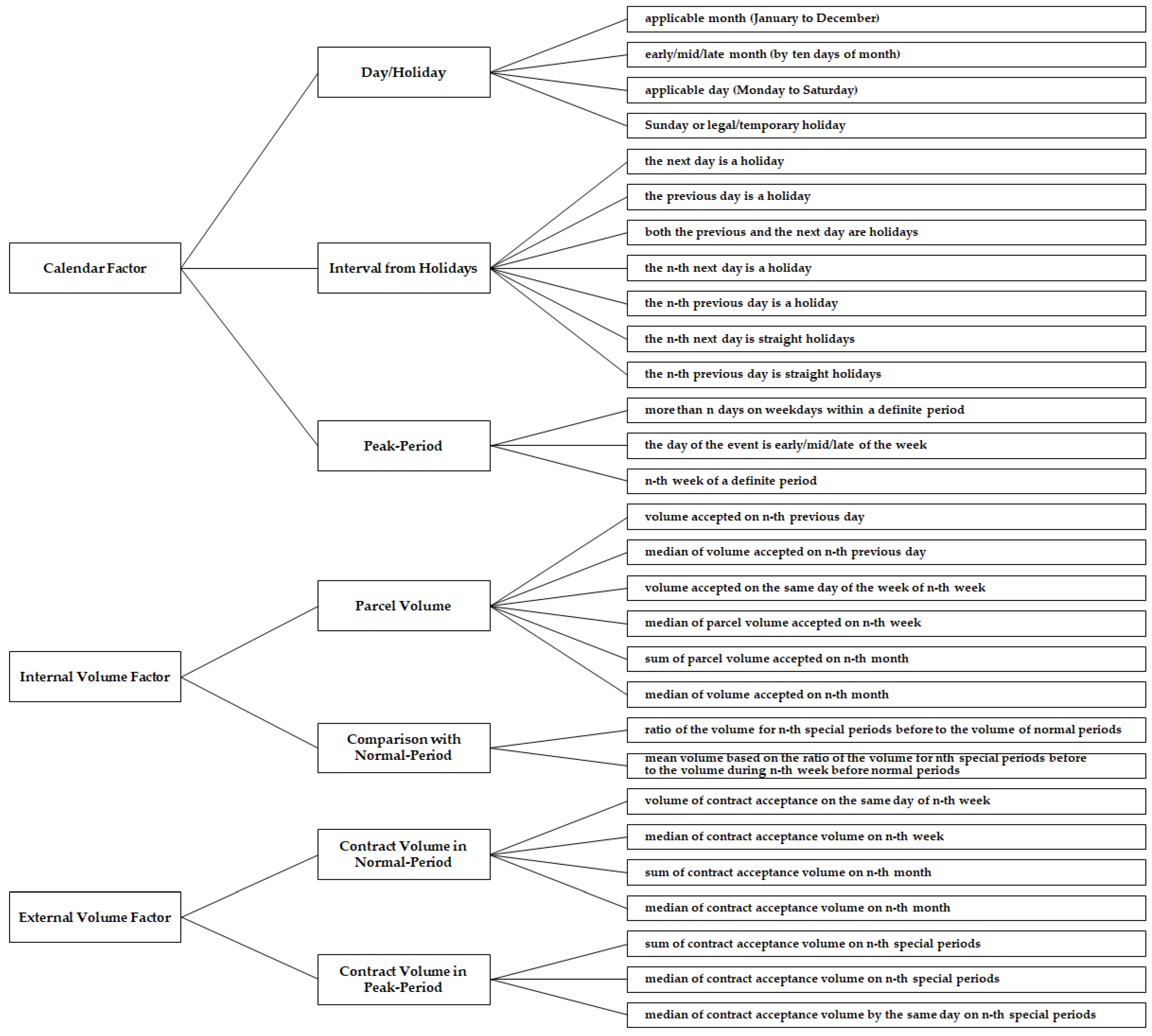
2.1. Feature Engineering

The data with the characteristic of repeatability in units of time include statistical self-similarity. Generally, it is possible to analyze the postal volume pattern depending on the characteristics repeated in units of time and calendar factors, such as day, weekend, holiday, and interval from holidays, to explore the statistical similarity.

In this study, the features of the patterns of parcel volume are categorized by internal and external factor-based derived features, as described in Figure 1 [14]. The internal features consist of calendar factors and volume similarity. From calendar and seasonal factors, we generate the features based on weekday, public holidays, and interval with holidays. The features of the time interval include the day before holidays, the day after holidays, and holidays that overlapped with workdays, n-th days before and after weekends or holidays interspersed with workdays for indicating the increasing volume trend near the particular periods. The volume factor-based derived features contain the past and recent volumes in normal and peak periods. The numerical features are extracted from internal historical data, including the moving average values of n-th previous weeks of a special period and mail volume compared to usual periods from an n-th week earlier. Moreover, the features based on external factors are created from the bulk mailing and contract volume. The prediction of bulk mailing volume tends to have a considerable variance depending on the contract customer’s business situation, whereby we extract explanatory features based on large volume mailing companies to enhance prediction performance. In the proposed weighted ensemble method, the generated internal volume-based features and external bulk mailing-based features are employed as input variables for the predictive models.

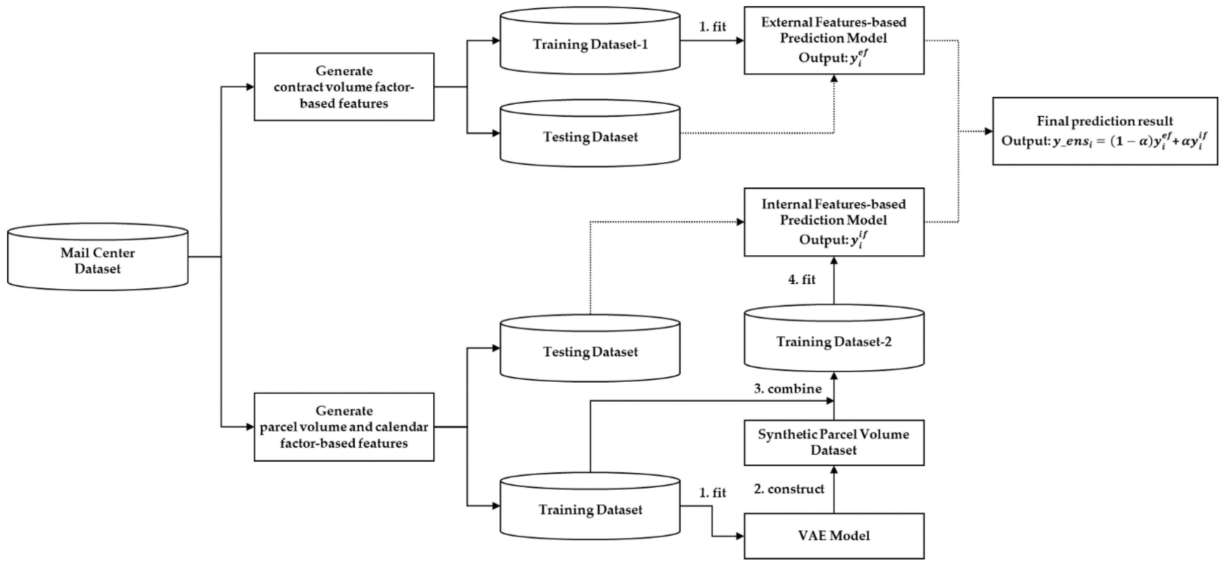
2.2. MLP-Based Weighted Ensemble Method

We propose an MLP-based demand prediction method for parcel logistics services. The proposed ensemble approach is designed for improving a single predictive model by combining two models based on the internal and external features with weight regulation, as shown in Figure 2. The two models are built on training datasets prepared differently, including Training Dataset-1 and Training Dataset-2. The final prediction result is estimated by averaging the outcome of each model based on the models’ weight. These models are built on training datasets prepared differently; Training Dataset-1 and Training Dataset-2, and the final prediction result is estimated by averaging the outcome of each model based on models’ weight.

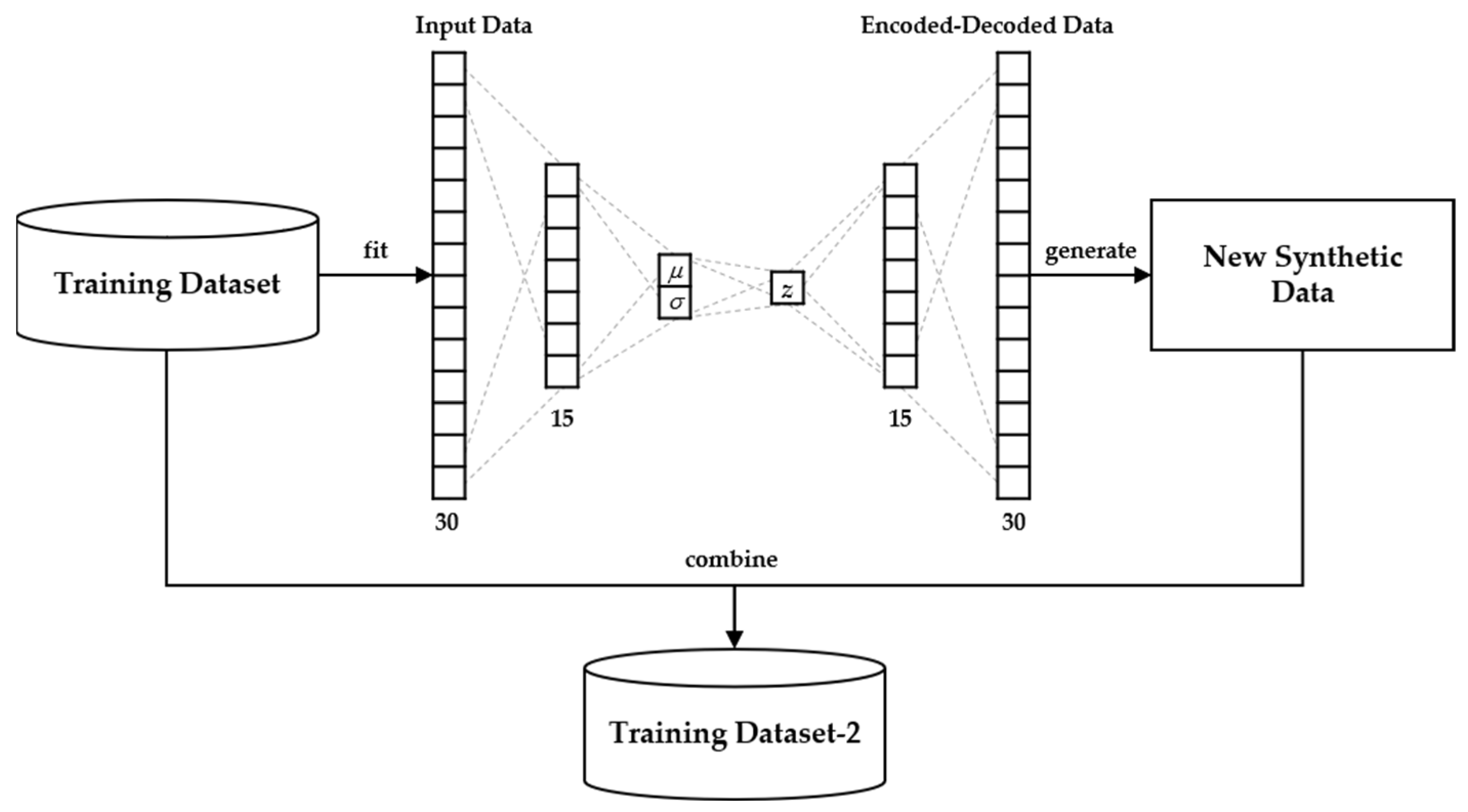
2.2.1. Construction of Training Datasets

Our proposed method is to predict the parcel volume during special periods of sharp changes in logistics services. The proposed method constructs two MLP models based on the generated internal and external features. These models are learned from datasets prepared differently from the initial mail center datasets. The first predictive model (external features-based prediction model shown in Figure 2) is to predict the total parcel volume during special periods. Therefore, the first training dataset is produced by grouping daily information into summary rows belonging to the holiday. The Training Dataset-1 consists of the external features based on the large volume mailing and contract customer data, and the target variable is estimated by the sum of parcel volume during a peak period of the particular holidays.

For the second training dataset, instead of using the initial daily dataset directly, we prepare an enriched training dataset named Training Dataset-2 by adding the 500 synthetic mailing data generated from the VAE model. The VAE model is excluded on the first training dataset, which is a summarized representation of the daily dataset because the compressed dataset is produced from the original dataset and may not be able to properly represent the original data distribution. Therefore, the VAE model is applied to the second training dataset construction.

The VAE is a neural network introduced first by [15]. It is mainly used to generate synthetic data. For example, in [16], the VAE was used to generate synthetic electronic health records. The effectiveness of the VAE was confirmed by the comparison of LSTM models trained on the synthetic and actual datasets. The authors of [17] proposed a coronary heart disease risk prediction method based on neural networks. They improved the prediction performance by augmenting rare instances with the VAE-based synthetic data. In [18], the VAE was used for image data generation and evaluated on the MNIST dataset. The VAE-based approach outperformed other traditional data generation methods, such as Synthetic Minority Over-sampling Technique (SMOTE) and Adaptive Synthetic (ADASYN).

Figure 3 presents an architecture of the VAE model used in this study. Generally, the architecture of the VAE involves encoder and decoder parts. The encoder part encodes input data as a latent distribution in a lower-dimensional space and learns to return the mean and variance for the normal distribution of data. Then, the random point sampled from that distribution is decoded, and an error between decoded data and the initial data is calculated to adjust model weights. To generate synthetic data from the trained VAE, first, a random point z is estimated by Equation (1):

$$z=\mu +\sigma \times \epsilon$$

(1)

where $\epsilon$ is randomly sampled from the standard normal distribution, and $\mu$ and $\sigma$ are the mean and standard deviations of the latent distribution. The sampled point $z$ is decoded to obtain new data.

Input and output layers of the VAE model in the proposed method consist of 30 nodes that represent input features for an internal factors-based model and its target variable. Each hidden layer with 15 nodes uses the ReLU activation function described in Equation (2):

$$\mathrm{ReLU}\left(x\right)=\{{}_{x if x>0}{}^{0 if x\le 0}=\max \left\{0,x\right\}$$

(2)

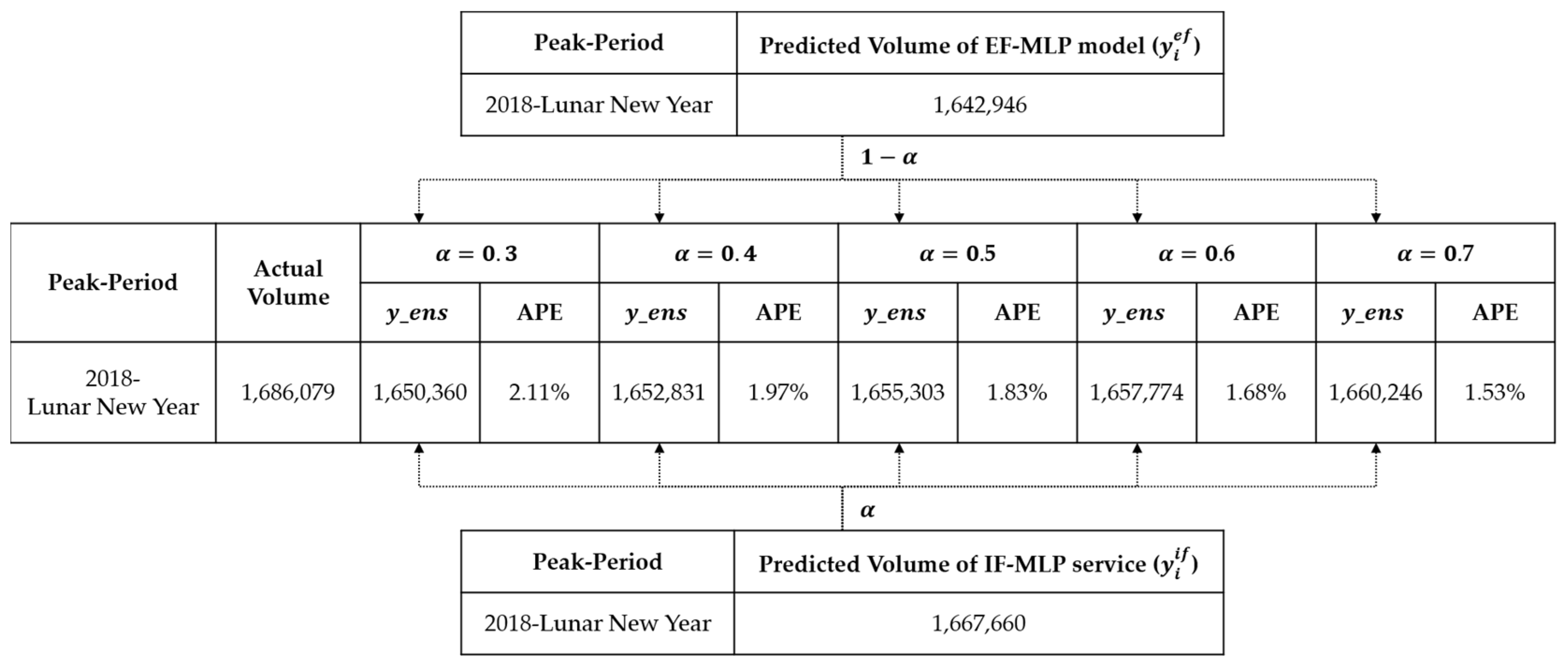
2.2.2. Ensembling MLP Models

The proposed ensemble method is built using the generated internal and external features and the artificial neural network (ANN) technique; the ANN implemented in this study is MLP. The neural network was first introduced by Warren McCullough and Walter Pitts in 1943 [19] and successfully used in many fields, such as natural language processing [20], image processing [21], recommendation systems [22], and so on.

It involves input, hidden, and output layers. Neurons of the input layer represent input variables, and neurons of hidden and output layers receive the weighted summation of neurons in their previous layer and transform it using activation functions. It is trained by changing the weight of each neuron to minimize the difference between the target value and predicted output.

In this study, we propose the weighted ensemble method by constructing two MLP models based on the extracted internal and external features. EF-MLP is built on the large volume of mailing and contract customer data-based external features to predict the total volume of parcel services during peak periods. IF-MLP is trained on calendar and internal volume-derived features. The structure of EF-MLP consists of two hidden layers with eight and two neurons, while two hidden layers of IF-MLP have 58 and 29 neurons. The ReLU activation function is used in all hidden layers. The results of each model are combined using Equation (3):

$$y\_en{s}_i=\left(1-\alpha \right)\times y_i^{ef}+\alpha \times y_i^{if}$$

(3)

where $y\_en{s}_i$ is the ensembled predicted value; $y_i^{ef}$ is the predicted value of the EF-MLP; $y_i^{if}$ is the predicted value of the IF-MLP; $\mathsf{\alpha }\left(0\le \alpha \le 1\right)$ is the weight for IF-MLP; and $(1-\mathsf{\alpha }$) is the weight for EF-MLP.

An example of the prediction process of the proposed ensemble method is demonstrated in Figure 4.

In the prediction procedure, the predictive results of the EF-MLP and IF-MLP models are given as an input value of the ensemble model for peak-period prediction. For the final prediction, the outputs of the proposed EF-MLP and IF-MLP models are combined based on the weight value. The proposed weighted ensemble method with internal and external factor-based derived features can prevent the prediction output from being inappropriately biased and complement for weaknesses of individual EF-MLP and IF-MLP models.

3. Experimental Study

The proposed method is validated on 25 Korean mail center datasets. We have compared the proposed method with other predictive methods widely used in previous studies. Moreover, we compared several MLP models that were trained on the differently prepared datasets to demonstrate how the proposed method can enhance the performance of the compared MLP models. In addition, we have experimented by replacing the MLP models in the proposed method with other compared prediction models to show that algorithms used in the proposed method work well together. The prediction performance is evaluated using MAE, RMSE, MAPE and SMAPE.

3.1. Experimental Dataset

The compared and proposed methods are validated on postal volume data from the Korea Post. The domestic mail service in South Korea is generally classified into ordinary mail service and parcel mail service. For the ordinary mail, Korea Post, which is a government agency responsible for providing postal services, handles letters. For the parcel mail, Korea Post engages with several logistic companies to provide stable services. The postal logistics process generally consists of four stages of acceptance, sorting, transportation, and delivery. The mail and logistics centers of Korea Post sort parcel and ordinary mail, which are to be transported through the exchange center or directly to the inbound mail centers of respective destinations. 24 mail centers are evenly distributed across the country and one exchange center is located at the center of the nationwide network.

This study used parcel mail datasets of 25 mail sorting and logistics centers including the exchange center. Datasets were collected from 1 September 2015 to 6 October 2020. Figure 5 shows the trend of the postal parcel volume from January to December 2019 at Mail Center #3 as an example. We can see that the total volume of parcel delivery services rose dramatically during the Lunar New Year and Korean Thanksgiving Day, which indicated in the shaded area of Figure 5.

The peak period is determined to be from the Monday two weeks before the start of a holiday until two working days after the last day of the holiday period. For example, assuming that the Lunar New Year 2020 is between January 24 and 27, its special period can be defined to be from January 6 to January 29. Datasets of special periods in 25 mail centers are summarized in

Table 1. Summary of datasets of peak periods in 25 mail centers.

Mail Center	Q1	Q2	Q3	Q4	Max	Avg	Stdev	95% CI	CV
Mail Center #1	52,842.5	120,541.0	149,959.0	225,370.0	225,370	104,943.7	63,352.7	95,096.4–114,790.9	0.60
Mail Center #2	2180.0	20,477.0	29,992.0	79,048.0	79,048	23,705.5	17,073.4	76,377.3–81,718.7	0.72
Mail Center #3	9889.0	28,064.0	38,370.0	77,927.0	77,927	26,459.0	16,882.7	23,814.6–29,103.4	0.64
Mail Center #4	27,063.0	47,586.0	58,418.0	139,060.0	139,060	45,200.8	26,463.4	40,973.9–49,427.7	0.59
Mail Center #5	24,075.5	41,184.5	51,461.3	94,285.0	94,285	37,884.1	22,435.9	34,288.6–41,479.6	0.59
Mail Center #6	6267.3	10,545.0	15,723.5	29,372.0	29,372	10,982.2	6737.3	8405.9–13,558.5	0.61
Mail Center #7	25,117.5	64,168.0	84,739.5	135,408.0	135,408	57,270.0	33,229.3	52,297.9–62,242.1	0.58
Mail Center #8	10,982.0	24,748.0	34,520.0	71,813.0	71,813	23,914.4	15,760.3	19,387.5–28,441.3	0.66
Mail Center #9	27,461.5	58,678.0	75,437.5	121,475.0	121,475	51,902.1	30,383.5	47,127.7–56,676.5	0.59
Mail Center #10	25,940.0	45,000.0	58,127.5	94,897.0	94,897	41,943.5	24,780.3	38,011.5–45,875.5	0.59
Mail Center #11	37,859.0	70,448.0	85,492.8	138,841.0	138,841	63,427.3	35,386.0	53,950.9–72,903.7	0.56
Mail Center #12	40,217.0	89,316.0	119,860.8	237,143.0	237,143	82,019.7	51,102.6	73,989.6–90,049.8	0.62
Mail Center #13	42,016.8	69,176.5	95,636.8	156,706.0	156,706	67,975.5	51,102.6	61,594.2–74,356.8	0.75
Mail Center #14	16,935.5	30,181.5	46,781.3	74,552.0	74,552	31,479.3	20,162.7	28,226.2–34,732.4	0.64
Mail Center #15	12,599.8	19,316.0	28,208.0	48,345.0	48,345	19,804.8	11,208.1	17,945.4–21,664.2	0.57
Mail Center #16	10,828.0	41,718.0	62,952.0	117,847.0	117,847	40,518.9	28,092.7	36,146.4–44,891.4	0.69
Mail Center #17	24,916.3	68,523.0	98,665.5	176,951.0	176,951	67,183.7	42,668.3	60,521.6–73,845.8	0.64
Mail Center #18	10,243.3	15,970.5	22,504.8	48,978.0	48,978	16,187.6	10,150.5	17,945.4–21,664.2	0.63
Mail Center #19	8630.0	18,777.0	33,069.0	70,283.0	70,283	21,526.0	15,927.7	18,911.5–24,140.5	0.74
Mail Center #20	11,396.8	21,525.0	29,665.8	54,976.0	54,976	20,651.3	12,261.1	18,699.4–22,603.2	0.59
Mail Center #21	11,008.0	20,151.0	30,727.0	69,885.0	69,885	21,959.8	15,357.4	19,473.6–24,446.0	0.70
Mail Center #22	25,305.0	70,339.0	85,875.0	151,727.0	151,727	62,182.4	38,329.0	19,473.6–24,446.0	0.62
Mail Center #23	13,141.5	24,884.5	46,106.0	89,609.0	89,609	29,871.5	22,499.3	26,265.8–33,477.2	0.75
Mail Center #24	7191.8	14,144.0	20,541.0	43,956.0	43,956	14,001.7	9061.1	12,529.8–15,473.6	0.65
Mail Center #25	40,091.5	91,905.0	147,942.5	222,904.0	222,904	93,499.4	62,742.8	83,794.9–03,203.9	0.67

Q1–Q4: from the first quartile to the fourth quartile; Max: maximum value; Avg: average value; Stdev: standard deviation; CI: confidence interval; CV: coefficient of variation.

.

3.2. Evaluation Metrics

To evaluate the prediction performance of the compared models, Mean Absolute Error (MAE), Root Mean Squared Error (RMSE), Symmetric Mean Absolute Percentage Error (SMAPE), and Mean Absolute Percentage Error (MAPE) metrics are used.

$$\mathrm{MAE}=\frac{1}{n}{\displaystyle \sum }_{i=1}^n\left|{\widehat{y}}_i-y_i\right|$$

(4)

$$\mathrm{RMSE}=\sqrt{\frac{1}{n}{\displaystyle \sum }_{i=1}^n{\left(y_i-{\widehat{y}}_i\right)}^2}$$

(5)

$$\mathrm{SMAPE}=\frac{1}{n}\left({\displaystyle \sum }_{i=1}^n\frac{\left|y_i-{\widehat{y}}_i\right|}{\left(y_i+{\widehat{y}}_i\right)/2}\right)\times 100$$

(6)

$$\mathrm{MAPE}=\frac{1}{n}\left({\displaystyle \sum }_{i=1}^n\left|\frac{{\widehat{y}}_i-y_i}{y_i}\right|\right)\times 100$$

(7)

where $n$ is number of the sample, ${\widehat{y}}_i$ is the i-th predicted value, and $y_i$ is the i-th actual value.

3.3. Compared Methods

We have compared the proposed method with other predictive methods using the Scikit-learn Python library, which contains implementations of machine learning and statistical modeling for classification, regression, and clustering [23]. The performance comparison was conducted with the commonly used techniques in previous studies.

Multiple Linear Regression (MLR) is commonly used for regression tasks [24]. It estimates coefficients that explain the correlation between the response and explanatory variables.

Least Absolute Shrinkage and Selection Operator (LASSO) is one kind of regularized linear regression. It minimizes the prediction error by shrinking the coefficients of some input variables that are irrelevant to the prediction task to zero [25].

Support Vector Regression (SVR) is a type of Support Vector Machine [26] used as a regression method. SVR works by using the ε-tube that best approximates the continuous-value function for balancing model complexity and prediction error [27]. We have built an SVR model with a C regularization parameter is equal to 0.1 and a linear kernel function.

Extreme Gradient Boosting (XGBoost) is an ensemble algorithm based on a decision tree and is formed on a gradient-boosting framework. It consists of multiple decision trees based on different subsets of features and combines their predictions to generate a final prediction. Each decision tree is built on the errors of the previous trees [28]. We have configured the learning rate to 0.3; the booster is gradient-boosting linear (gblinear), and the number of boosting iterations is 100.

Random Forest (RF) is widely used in classification and regression tasks. It builds several decision trees on dissimilar sub-samples from the training dataset. In the case of regression, the final result is generated by their average [29]. We set the number of trees to 500.

Long Short-Term Memory (LSTM) is one kind of Recurrent Neural Network (RNN) used in sequence processing [30]. It solves the problem of RNN that cannot predict accurately from the long-term information by extending the memory cells using input, forget and output gates. Those gates are employed to add useful information to the cell (input gate), remove unnecessary information from the cell (forget gate), and extract applicable information from the current cell (output gate). The LSTM model used in the experimental study had a single hidden layer with 16 neurons. The model was trained with Adam optimizer [31], batch size to 16, epochs to 100, and learning rate to 0.001.

Multilayer Perceptron (MLP) constructs multiple hidden layers in between input and output layers [19]. Each layer consists of artificial neurons connected with its following layers’ neurons by weight parameters. The weight parameters are optimized by the back-propagation algorithm. The training configuration of the MLP was Adam optimizer, batch size to 16, epochs to 100, and learning rate to 0.001.

3.4. Prediction Results

We compared seven prediction models, such as MLR, LASSO, SVR, RF, XGBoost, LSTM, and MLP with the proposed method on 25 mail center datasets to predict postal parcel volume during special periods. We selected the special periods for the training dataset from Korean Thanksgiving Day 2016 to the target peak period. For example, holidays that started from the Korean Thanksgiving Day 2016 to the Lunar New Year 2018 were used to train the model that predicts the 2018 Korean Thanksgiving Day. Figure 6 shows a visualization of the train-test split.

Foremost, we compared several MLP models that were trained on the differently prepared training datasets to demonstrate how the proposed method can enhance the performance of compared MLP models.

Table 2. Performance of MLP models by the proposed method on the 25 mail center datasets.

Mail Centers	MLP (Baseline)		EF-MLP		IF-MLP		Proposed
	MAPE	MAE	MAPE	MAE	MAPE	MAE	MAPE	MAE
	SMAPE	RMSE	SMAPE	RMSE	SMAPE	RMSE	SMAPE	RMSE
Mail Center #1	8.245	166,430.0	9.237	201,634.5	5.923	128,320.7	6.076	131,779.3
	8.679	187,880.7	10.055	274,179.0	6.211	166,883.6	6.386	172,273.1
Mail Center #2	24.860	129,159.6	23.368	121,265.9	25.401	132,437.6	24.108	269,291.7
	63.978	454,463.6	72.296	432,934.8	63.379	421,951.1	62.094	394,716.5
Mail Center #3	12.122	55,555.2	10.705	53,918.7	7.528	34,675.2	10.090	50,429.3
	11.689	58,175.8	11.085	68,097.4	7.262	45,449.9	10.348	62,254.3
Mail Center #4	10.864	84,690.7	11.847	77,226.4	7.503	64,445.3	8.931	56,224.0
	10.838	98,681.0	10.530	110,427.5	7.844	88,154.4	8.060	85,958.8
Mail Center #5	12.212	85,184.9	8.209	60,226.8	8.672	58,807.0	7.868	54,813.0
	13.121	96,738.0	8.865	81,912.7	9.201	67,044.5	8.287	60,962.6
Mail Center #6	13.931	26,250.5	8.827	16,598.3	8.060	14,978.9	3.225	6180.1
	15.186	28,240.1	8.571	20,286.1	8.683	19,855.1	3.287	6711.9
Mail Center #7	15.890	184,636.9	7.939	110,440.1	12.971	157,518.5	7.661	101,561.9
	15.703	203,238.7	8.842	189,087.5	12.821	185,911.8	8.362	167,814.1
Mail Center #8	12.959	53,347.1	9.084	39,366.6	15.951	63,867.6	8.424	36,017.7
	12.982	65,448.9	9.669	47,857.7	14.375	76,470.0	8.795	42,160.4
Mail Center #9	8.944	88,769.8	12.547	115,290.7	6.324	63,180.8	11.263	104,454.8
	9.109	94,215.5	12.226	145,732.4	6.763	89,717.9	11.098	122,761.0
Mail Center #10	8.126	66,934.4	12.113	106,297.9	2.663	22,661.2	7.382	64,424.7
	8.322	70,176.0	13.241	128,728.4	2.738	34,506.1	7.788	78,741.3
Mail Center #11	8.173	93,854.9	3.635	41,706.9	5.980	66,280.8	3.171	35,222.8
	7.895	109,198.8	3.609	48,269.8	5.919	73,963.2	3.105	48,512.5
Mail Center #12	12.548	213,895.2	15.592	291,748.6	12.500	216,383.2	13.304	231,382.9
	13.530	239,177.6	17.471	353,703.2	13.598	262,091.1	14.478	271,213.8
Mail Center #13	11.340	132,817.0	9.589	120,317.4	10.735	134,590.5	8.539	106,148.2
	10.696	182,117.9	9.891	144,527.3	10.522	155,959.6	8.692	122,585.5
Mail Center #14	11.617	68,646.8	7.010	44,892.1	10.772	64,262.8	6.926	44,347.8
	12.077	86,639.6	7.668	77,396.3	15.118	89,138.0	7.580	76,730.7
Mail Center #15	9.665	30,503.0	4.042	12,698.1	7.798	24,605.1	3.733	11,624.5
	9.519	33,665.8	3.965	13,690.6	7.868	27,276.8	3.669	12,610.5
Mail Center #16	8.135	63,139.3	6.866	52,967.8	4.185	32,533.2	3.398	26,809.2
	7.801	72,776.7	6.964	61,500.6	4.359	43,777.2	3.478	31,514.6
Mail Center #17	18.482	210,939.7	10.730	113,781.4	11.529	126,172.2	10.083	105,712.6
	18.849	232,308.3	9.736	150,959.2	10.877	156,001.1	9.175	145,372.9
Mail Center #18	29.400	74,301.1	16.129	39,864.5	14.355	36,356.8	11.235	27,723.7
	24.262	96,851.9	13.851	57,401.9	14.867	41,707.7	10.197	37,596.3
Mail Center #19	15.222	52,095.2	4.648	15,539.0	11.379	38,471.7	4.545	15,262.0
	13.964	74,066.8	4.461	22,703.4	10.739	48,963.5	4.319	24,065.9
Mail Center #20	6.375	23,599.9	8.152	34,187.4	5.291	19,475.2	5.249	19,756.7
	6.319	33,965.6	8.957	53,419.3	5.198	25,839.9	5.202	23,838.8
Mail Center #21	16.660	54,886.0	49.398	169,356.8	11.771	39,135.7	13.203	44,925.5
	16.030	61,489.4	35.081	246,618.6	11.418	49,462.3	12.227	52,351.9
Mail Center #22	14.900	183,708.7	9.093	106,237.1	11.342	133,792.7	10.739	126,154.0
	16.069	221,819.3	8.774	130,242.2	11.524	136,342.5	10.790	130,241.2
Mail Center #23	29.869	146,433.4	21.777	99,925.7	17.243	77,933.3	15.276	69,954.8
	30.531	179,673.1	20.077	119,480.9	15.575	94,092.7	13.882	91,474.5
Mail Center #24	12.186	30,362.3	17.649	47,736.3	10.314	27,247.0	10.688	28,141.9
	13.265	34,953.7	20.052	56,824.1	10.893	30,520.6	11.518	32,974.8
Mail Center #25	28.113	403,099.3	9.804	145,090.0	23.176	333,733.9	21.303	306,970.0
	22.685	539,578.5	9.232	186,659.0	19.928	407,434.7	18.459	379,725.5

shows the prediction performance of compared MLP models for each mail center, and the best results are emphasized. The prediction results show that the proposed external and internal MLP model-based weighted ensemble method outperforms other MLP models on 13 of 25 mail center datasets.

From Table 2, the EF-MLP model performed better than the baseline MLP model using the initial dataset on most of the mail center datasets, and its average MAPE was less than the baseline MLP model by 4.98%. Moreover, the MAPE of the IF-MLP model was decreased by enriching the training dataset using synthetic data generated from the VAE model, and its average MAPE dropped to 10.77% compared with the MAPE of the baseline MLP model of 14.43%. Moreover, the average MAE, RMSE, SMAPE, and MAPE of the proposed model ensembling EF-MLP and IF-MLP models with the weight were less than the baseline MLP model by 25,917.1, 35,215.1, 4.87%, and 4.98%, respectively. Finally, the proposed method was superior to the baseline MLP model in giving the minimum errors. For each mail center, we selected the different weights for EF-MLP and IF-MLP based on the training performance of the proposed method.

Table 3. Comparison of MAPE, SMAPE, RMSE and MAE results.

Mail Centers	MLR		LASSO		SVR		XGBoost		RF		LSTM		Proposed
	MAPE	MAE	MAPE	MAE	MAPE	MAE	MAPE	MAE	MAPE	MAE	MAPE	MAE	MAPE	MAE
	SMAPE	RMSE	SMAPE	RMSE	SMAPE	RMSE	SMAPE	RMSE	SMAPE	RMSE	SMAPE	RMSE	SMAPE	RMSE
Mail Center #1	8.700	176,927.2	8.800	183,267.9	8.300	168,968.4	7.000	143,238.6	5.960	120,928.2	9.581	198,052.7	8.200	166,430.0
	9.145	196,286.1	9.189	197,004.6	8.583	185,988.8	7.259	165,407.9	6.064	129,216.5	10.096	216,752.1	8.679	187,880.7
Mail Center #2	25.567	133,309.2	23.104	120,387.0	24.855	125,101.1	21.061	109,000.7	29.904	154,773.0	23.854	120,888.3	24.860	129,159.6
	63.978	454,463.6	61.039	436,652.9	62.794	404,836.7	58.927	432,818.1	68.399	338,071.0	62.385	457,488.2	63.129	470,150.7
Mail Center #3	13.210	59,803.5	8.622	37,953.7	9.632	44,434.8	8.357	37,345.6	15.507	73,843.5	11.806	55,294.1	12.122	55,555.2
	12.248	70,960.9	7.859	58,173.2	9.507	54,156.0	7.701	53,794.7	15.200	85,141.4	11.572	60,555.8	11.689	58,175.8
Mail Center #4	8.718	55,153.8	4.745	35,652.1	13.292	96,957.7	6.313	46,961.0	8.498	61,704.6	11.704	86,176.1	10.864	84,690.7
	8.321	71,366.8	4.780	38,827.4	14.301	110,275.6	6.456	53,920.5	8.428	64,974.4	12.633	98,993.6	10.838	98,681.0
Mail Center #5	9.194	65,580.1	11.130	80,354.2	12.606	88,449.8	11.616	84,341.6	11.833	81,396.0	10.640	71,789.6	12.212	85,184.9
	9.783	77,081.5	11.384	84,720.1	12.808	93,646.0	11.523	87,613.7	12.706	90,280.7	11.585	86,332.0	13.121	96,738.0
Mail Center #6	8.670	16,416.9	10.357	19,485.0	16.509	31,091.2	11.469	21,543.6	7.841	14,572.3	14.307	27,009.9	13.931	26,250.5
	9.083	16,707.0	11.063	21,319.8	18.438	34,405.9	12.406	24,283.3	8.501	20,282.9	15.657	29,265.2	15.186	28,240.1
Mail Center #7	15.614	194,105.6	15.764	193,784.9	14.380	172,578.1	14.595	178,457.5	17.170	206,847.0	16.436	200,644.4	15.890	184,636.9
	16.107	230,523.0	16.147	223,426.7	14.253	201,953.4	14.725	203,967.5	17.928	239,378.5	16.463	237,349.5	15.703	203,238.7
Mail Center #8	12.150	47,857.8	14.685	58,537.6	14.172	58,134.2	16.385	66,464.3	9.754	39,491.3	8.216	33,513.9	12.959	53,347.1
	11.680	57,534.7	13.697	67,064.5	12.934	69,725.4	14.565	82,339.2	9.778	45,368.2	8.014	38,377.6	12.982	65,448.9
Mail Center #9	15.475	154,923.6	13.724	139,705.0	11.173	112,467.8	13.898	139,276.6	10.044	96,345.6	9.106	94,373.0	8.944	88,769.8
	16.323	172,577.8	13.677	154,132.8	11.662	137,145.2	13.838	155,917.5	10.461	107,908.6	9.363	107,343.3	9.109	94,215.5
Mail Center #10	9.718	84,693.5	7.865	66,159.7	3.734	31,769.3	6.467	51,486.4	9.532	76,688.4	6.447	58,445.7	8.126	66,934.4
	10.324	106,016.5	7.804	74,191.2	3.768	41,944.2	6.381	59,493.8	10.090	86,767.4	6.801	79,742.1	8.322	70,176.0
Mail Center #11	7.684	86,461.5	6.946	78,909.5	10.479	120,436.2	8.428	97,234.5	8.207	94,408.1	4.796	52,858.0	8.173	93,854.9
	7.624	89,752.8	6.777	84,003.9	10.117	129,083.6	8.114	110,128.6	8.001	113,977.8	4.792	65,940.2	7.895	109,198.8
Mail Center #12	10.909	198,019.9	11.528	185,539.0	11.335	198,073.9	8.060	150,602.6	16.509	274,021.5	15.502	262,408.4	12.548	213,895.2
	11.772	246,448.9	12.531	218,863.7	12.257	245,098.6	8.656	215,053.7	18.237	301,877.6	16.933	282,917.5	13.530	239,177.6
Mail Center #13	10.859	129,566.8	6.434	74,832.8	9.337	113,476.0	9.281	114,457.0	7.296	85,524.0	8.080	98,972.2	11.340	132,817.0
	11.120	138,456.2	6.335	99,743.8	9.057	133,681.6	8.935	136,944.4	7.062	107,624.9	7.967	120,164.5	10.696	182,117.9
Mail Center #14	16.932	96,731.0	18.979	107,594.1	19.794	110,870.1	20.317	114,463.1	11.588	66,490.6	13.838	78,714.7	11.617	68,646.8
	16.959	118,159.9	18.727	127,884.7	18.542	146,544.5	19.714	137,958.4	11.370	84,755.5	13.502	99,496.8	12.077	86,639.6
Mail Center #15	8.754	27,941.4	11.134	35,581.8	13.548	43,346.5	14.943	47,741.2	15.315	48,570.3	11.348	35,829.2	9.665	30,503.0
	8.690	32,400.6	11.092	41,586.6	13.484	52,510.2	14.895	54,839.4	14.685	54,990.4	10.834	40,745.5	9.519	33,665.8
Mail Center #16	3.698	28,663.5	5.464	43,052.0	6.492	51,490.9	6.490	51,788.5	6.349	47,643.9	7.297	56,151.7	8.135	63,139.3
	3.816	36,871.1	5.561	46,735.1	6.427	55,291.6	6.305	61,412.2	7.075	83,335.8	7.355	61,467.2	7.801	72,776.7
Mail Center #17	14.733	158,789.7	16.539	183,795.1	16.429	186,916.6	14.200	161,566.7	19.331	161,566.7	16.563	183,237.2	18.482	210,939.7
	13.463	196,929.1	15.824	220,976.3	16.195	207,466.2	13.491	190,206.8	18.517	240,885.5	15.926	204,504.1	18.849	232,308.3
Mail Center #18	20.435	51,450.7	21.996	55,775.9	25.215	64,258.0	19.346	49,369.6	15.841	40,561.3	21.873	55,301.3	29.400	74,301.1
	28.192	79,467.2	26.368	70,379.0	22.703	69,386.8	18.473	56,735.1	14.867	47,297.2	25.580	68,735.8	24.262	96,851.9
Mail Center #19	15.019	51,420.0	15.848	54,138.4	14.909	50,633.0	18.489	62,803.5	12.916	44,291.3	13.166	44,567.9	15.222	52,095.2
	13.911	65,230.5	14.368	73,624.5	13.558	69,627.7	16.082	87,969.5	12.076	56,959.1	12.230	56,548.1	13.964	74,066.8
Mail Center #20	11.547	45,280.7	11.540	45,856.9	10.177	40,072.3	11.494	45,175.6	7.627	28,476.7	7.115	26,853.6	6.375	23,599.9
	11.300	54,913.2	10.861	57,032.3	9.892	47,984.0	10.965	55,129.5	7.344	37,455.5	6.967	32,726.6	6.319	33,965.6
Mail Center #21	16.681	60,290.4	16.351	57,179.8	13.080	44,519.4	16.823	61,666.8	24.834	92,035.0	12.517	39,110.7	16.660	54,886.0
	14.947	72,309.0	15.399	67,283.7	13.021	49,189.5	15.435	70,936.8	24.361	115,086.2	11.942	50,038.0	16.030	61,489.4
Mail Center #22	13.315	156,021.0	12.662	145,766.2	13.516	157,752.1	13.456	156,104.2	9.676	112,407.9	12.311	144,273.1	14.900	183,708.7
	13.954	176,387.5	12.670	173,683.7	13.815	171,023.6	13.699	174,139.7	9.571	124,694.2	12.691	161,564.8	16.069	221,819.3
Mail Center #23	20.367	93,087.6	21.404	98,199.6	17.038	78,316.0	20.242	91,943.1	24.992	111,352.3	17.995	80,754.6	29.869	146,433.4
	18.357	105,324.3	19.417	105,831.9	15.795	89,847.6	18.188	102,284.2	21.546	130,080.3	16.291	95,857.8	30.531	179,673.1
Mail Center #24	9.957	26,785.1	11.388	30,247.6	10.294	27,316.7	12.451	33,483.7	10.569	26,705.3	9.116	23,761.7	12.186	30,362.3
	10.261	30,556.2	11.716	32,659.0	10.588	29,210.4	12.606	35,745.9	11.103	27,769.1	9.721	28,603.8	13.265	34,953.7
Mail Center #25	26.521	380,001.1	27.421	393,419.5	28.329	404,349.9	29.513	415,541.1	26.655	386,851.2	22.264	323,511.7	28.113	403,099.3
	22.250	469,426.9	22.883	485,654.4	22.995	527,813.4	23.557	550,621.2	23.253	456,895.5	19.459	391,006.8	22.685	539,578.5

shows the performance comparison between the proposed method and the individual predictive methods. For 25 mail center datasets, ten centers have a higher coefficient of variation than the average, and the names of these mail centers are bolded in Table 3. The performance of our proposed method tends to be better for mail centers with large fluctuations. Among mail centers with a high coefficient of variation, the bolded highlight indicates that the proposed method is excellent. As shown from the MAPE, SMAPE, RMSE, and MAE results of Table 3, the proposed weighted ensemble method gave better performance than other individual compared models for most mail centers. The proposed method achieved better accuracy in MAPE and SMAPE than the MLR-based, LASSO-based, SVR-based, XGBoost-based, RF-based, and LSTM-based methods. It dropped MAPE and SMAPE values from MLR, LASSO, SVR, XGBoost, RF and LSTM-based methods by 3.9%, 3.9%, 4.5%, 4.2%, 4.3%, 3.2% and 4.1%, 3.8%, 4.2%, 3.7%, 4.2%, 3.4%, respectively. For the MAE and RMSE results, the proposed ensemble method outperformed the compared methods by giving 83,012.5 of MAE and 147,883.2 of RMSE on average. Its MAE value is less than the compared methods by 20,158.7, 17,994.5, 21,858.7, 18,269.8, 18,887.3, 15,087.2, and RMSE is lower by 29,240.3, 26,028.4, 29,411.1, 31,937.6, 17,351.2, 20,666.6, and 42,155.1, respectively.

Figure 7 represents the average performance of the compared methods on the 25 mail center datasets. Compared to ensemble methods constructed by the internal and external features-based compared algorithms, the ensemble model of the proposed method showed more accurate performance in MAPE by 25.2% up to 34.5%. For the MAE results, our prediction scheme for peak periods achieved improved accuracy by 15.4% up to 23.8% compared to the other methods. For the SMAPE and RMSE results, the proposed ensemble method outperformed the compared methods by reducing 24.0% up to 30.8% of SMAPE and by 10.5% up to 22.2% of RMSE, respectively.

Figure 8 shows the prediction performance of the proposed ensemble method using the enriching dataset based on VAE. We have experimented by replacing the MLP models in the proposed method with other compared prediction algorithms to show that algorithms used in the proposed method work well together. From Figure 8, we can see that the VAE-based data enrichment improved the average MAPE of all versions of weighted ensemble methods successfully. Moreover, the proposed MLPs-based weighted ensemble method learned from the enriched training dataset outperformed all weighted methods based on the MLR, LASSO, SVR, XGBoost, RF, and LSTM. In particular, our prediction scheme for peak periods demonstrated better performance compared with other predictive models by 21.9% on average, as shown in Figure 8.

As a result of the experimental study on Korean postal parcel datasets, the proposed method improved the prediction performance in terms of the MAPE reduction rate up to 59.6% compared to other methods during peak periods, such as the Lunar New Year and Korean Thanksgiving Day, when demand for logistics services increases sharply.

4. Conclusions

It is important to predict peak-period demand accurately to optimize the resource and operation in logistics industries. Korea Post, the national postal service provider, needs to predict short-term changes in parcel volume in order to optimize its operations, especially during periods of sharp changes in parcel volume.

This study proposed the prediction method for the demand of logistics services during special periods in holidays using deep learning models. The proposed method improved the prediction performance by two steps. In the first step, the training dataset was enriched by synthetic data generated from the VAE model. It decreased the average MAPE of the baseline MLP model that was learned from the daily training datasets of 25 mail centers by 3.7% (see the results of baseline MLP and IF-MLP in Table 2). In the second step, the proposed method combined two MLP models that were trained on the enriched daily training dataset using calendar and internal volume-derived features and the dataset using external features of the bulk mailing volume and contract customer data. The final prediction result was estimated by the weighted average of the outputs of these EF-MLP and IF-MLP models. The weighted ensemble of EF-MLP and IF-MLP models reduced the MAPE of the baseline MLP models by 5.0% successfully.

The experimental results showed how the proposed method improved the prediction performance step by step and compared the forecasting results of the proposed method with machine learning-based models on 25 mail center datasets. The proposed method outperformed the compared models on most datasets and achieved a performance improvement of up to 59.6%. The experimental results confirm that the proposed weighted ensemble model is acceptable for peak-period prediction, and it is highly possible to expand the range of its applications.

References

1. Fève, F.; Floren, J.P.; Rodriguez, F.; Soteri, S. Forecasting mail volumes in an evolving market environment. In Heightening Competition in the Postal and Delivery Sector, 1st ed.; Edward Elgar: Northampton, MA, USA, 2010; pp. 116–134. [Google Scholar] [CrossRef] [Green Version]
2. Toshkollari, O.; Sota, F.; Shtino, V.; Bozhiqi, K. Analysis and prediction of city postal services in Albania. A case study. In Proceedings of the UBT International Conference, Durres, Albania, 28–30 October 2016. [Google Scholar] [CrossRef] [Green Version]
3. Ebbesson, M. Mail Volume Forecasting an Evaluation of Machine Learning Models. Master’s Thesis, Uppsala University, Uppsala, Sweden, 2016. [Google Scholar]
4. Huang, L.; Xie, G.; Zhao, W.; Gu, Y.; Huang, Y. Regional logistics demand forecasting: A BP neural network approach. Complex Intell. Syst. 2021, 7, 1–16. [Google Scholar] [CrossRef]
5. Kim, E.; Jung, H. Feature Engineering-based Short-Term Prediction Model for Postal Parcel Logistics. In Proceedings of the 6th International Conference on Machine Learning Technologies, Jeju Island, Republic of Korea, 23–25 April 2021. [Google Scholar] [CrossRef]
6. Trinkner, U.; Grossmann, M. Forecasting Swiss mail demand. In Progress Toward Liberalization of the Postal and Delivery Sector, 1st ed.; Springer: Boston, MA, USA, 2006; Volume 49, pp. 267–280. [Google Scholar] [CrossRef]
7. Nguyen, T.Y. Research on logistics demand forecast in southeast Asia. World J. Eng. Technol. 2020, 8, 249–256. [Google Scholar] [CrossRef]
8. Rogan, I.D.; Pronić-Rančić, O.R. Forecasting the volume of postal services using Savitzky-Golay filter modification. In Proceedings of the 56th International Scientific Conference on Information, Communication and Energy Systems and Technologies, Sozopol, Bulgaria, 16–18 June 2021. [Google Scholar] [CrossRef]
9. Machado, C.; Silva, F. Postal Traffic in Portugal: Applying Time Series Modeling. In The Changing Postal Environment, 1st ed.; Springer: Cham, Switzerland, 2020; pp. 197–212. [Google Scholar] [CrossRef]
10. Pu, Z.; Yang, L.; Guo, Z.G. Applied Research on Logistics Demand Prediction Based on Support Vector Machine of Genetic Algorithm. In Proceedings of the International Conference on Computational and Information Sciences, Chengdu, China, 21–23 October 2011. [Google Scholar] [CrossRef]
11. Yu, N.; Xu, W.; Yu, K.L. Research on regional logistics demand forecast based on improved support vector machine: A case study of Qingdao city under the New Free Trade Zone Strategy. IEEE Access 2020, 8, 9551–9564. [Google Scholar] [CrossRef]
12. Rogan, I.D.; Pronić-Rančić, O.R. SARIMA and ANN Approaches in Forecasting the Volume of Postal Services. In Proceedings of the 15th International Conference on Advanced Technologies, Systems and Services in Telecommunications, Nis, Serbia, 20–22 October 2021. [Google Scholar] [CrossRef]
13. Lin, Y.S.; Zhang, Y.; Lin, I.C.; Chang, C.J. Predicting logistics delivery demand with deep neural networks. In Proceedings of the 7th International Conference on Industrial Technology and Management, Oxford, UK, 7–9 March 2018. [Google Scholar] [CrossRef]
14. Kim, E.; Jung, H. Extreme Event Forecasting for Postal Logistics Service. In Proceedings of the 8th International Conference on Management of e-Commerce and e-Government, Jeju, Republic of Korea, 4–6 July 2021. [Google Scholar] [CrossRef]
15. Kingma, D.P.; Welling, M. Auto-Encoding Variational Bayes. arXiv 2013, arXiv:1312.6114. [Google Scholar]
16. Biswal, S.; Ghosh, S.; Duke, J.; Malin, B.; Stewart, W.; Sun, J. EVA: Generating Longitudinal Electronic Health Records Using Conditional Variational Autoencoders. arXiv 2020, arXiv:2012.10020. [Google Scholar]
17. Amarbayasgalan, T.; Pham, V.H.; Theera-Umpon, N.; Piao, Y.; Ryu, K.H. An efficient prediction method for coronary heart disease risk based on two deep neural networks trained on well-ordered training datasets. IEEE Access 2021, 9, 135210–135223. [Google Scholar] [CrossRef]
18. Wan, Z.; Zhang, Y.; He, H. Variational autoencoder based synthetic data generation for imbalanced learning. In Proceedings of the IEEE Symposium Series on Computational Intelligence (SSCI) 2017, Honolulu, HI, USA, 27 November 2017–1 December 2017. [Google Scholar] [CrossRef]
19. Jain, A.K.; Mao, J.; Mohiuddin, K.M. Artificial neural networks: A tutorial. Computer 1996, 29, 31–44. [Google Scholar] [CrossRef] [Green Version]
20. Otter, D.W.; Medina, J.R.; Kalita, J.K. A survey of the usages of deep learning for natural language processing. IEEE Trans. Neural Netw. Learn. Syst. 2020, 32, 604–624. [Google Scholar] [CrossRef] [PubMed] [Green Version]
21. Litjens, G.; Kooi, T.; Bejnordi, B.E.; Setio, A.A.A.; Ciompi, F.; Ghafoorian, M.; Van Der Laak, J.A.; Van Ginneken, B.; Sánchez, C.I. A survey on deep learning in medical image analysis. Med. Image Anal. 2017, 42, 60–88. [Google Scholar] [CrossRef] [PubMed] [Green Version]
22. Zhang, S.; Yao, L.; Sun, A.; Tay, Y. Deep learning based recommender system: A survey and new perspectives. ACM Comput. Sur. 2019, 52, 1–38. [Google Scholar] [CrossRef] [Green Version]
23. Pedregosa, F.; Varoquaux, G.; Gramfort, A.; Michel, V.; Thirion, B.; Grisel, O.; Blondel, M.; Prettenhofer, P.; Weiss, R.; Dubourg, V.; et al. Scikit-learn: Machine learning in Python. J. Mach. Learn. Res. 2011, 12, 2825–2830. [Google Scholar]
24. Kleinbaum, D.G.; Kupper, L.L.; Muller, K.E.; Nizam, A. Applied Regression Analysis and Other Multivariable Methods, 4th ed.; Cengage Learning: Boston, MA, USA, 2007. [Google Scholar]
25. Tibshirani, R. Regression shrinkage and selection via the lasso. J. R. Stat. Soc. Ser. B Stat. Methodol. 1996, 58, 267–288. [Google Scholar] [CrossRef]
26. Vapnik, V. The Nature of Statistical Learning Theory, 2nd ed.; Springer: Berlin, Germany, 2013. [Google Scholar]
27. Awad, M.; Khanna, R. Support vector regression. In Efficient Learning Machines, 1st ed.; Apress: Berkeley, CA, USA, 2015; pp. 67–80. [Google Scholar]
28. Chen, T.; Guestrin, C. Xgboost: A scalable tree boosting system. In Proceedings of the 22nd ACM SIGKDD International Conference on Knowledge Discovery and Data Mining, San Francisco, CA, USA, 13–17 August 2016. [Google Scholar] [CrossRef] [Green Version]
29. Breiman, L. Random forests. Mach. Learn. 2001, 45, 5–32. [Google Scholar] [CrossRef] [Green Version]
30. Hochreiter, S.; Schmidhuber, J. Long short-term memory. Neural Comput. 1997, 9, 1735–1780. [Google Scholar] [CrossRef] [PubMed]
31. Kingma, D.P.; Ba, J. Adam: A method for stochastic optimization. arXiv 2014, arXiv:1412.6980. [Google Scholar]
Figure 1. Feature-set by internal and external factors.
Applsci 12 11962 g001
Figure 2. Overall architecture of the proposed method. Dashed lines indicate prediction process; solid lines indicate training procedure.
Applsci 12 11962 g002
Figure 3. Architecture of the VAE model.
Applsci 12 11962 g003
Figure 4. Example of the prediction procedure based on two MLP models; APE: Absolute Percentage Error.
Applsci 12 11962 g004
Figure 5. Example of postal parcel data of a mail center.
Applsci 12 11962 g005
Figure 6. Train-test split; LNY: Lunar New Year, KTD: Korean Thanksgiving Day.
Applsci 12 11962 g006
Figure 7. Average performance of compared methods on 25 mail center datasets.
Applsci 12 11962 g007
Figure 8. Comparison of MAPE results of weighted ensemble methods based on initial and VAE-based enriched datasets.
Applsci 12 11962 g008