Dynamic Heat Transfer Calculation for Ground-Coupled Floor in Emergency Temporary Housing

Featured Application

A new heat transfer calculation method for ground-coupled floors was established. This method was applied particularly to temporary emergency housing. Results showed it was more efficient than the finite volume method. The effects of initial soil temperature were not ignorable in hot and cold climates. Insulation could slow down but not prevent the heat release of soil.

Abstract

Generally, ground-coupled floor heat transfer is supposed as annual periodic, which is reasonable for conventional buildings. However, for emergency housing with a short life cycle, the influence of initial soil temperature needs to be considered. In a previous study, the Wiener–Hopf technique was introduced to solve the two-dimensional transient heat transfer equation with mixed Dirichlet and Robin boundary conditions. Based on that, an analytical solution of the dynamic heat transfer equation with initial soil temperature conditions was obtained. Since the solution was in the form of a double integral, its numerical evaluation method was also analyzed to improve computational efficiency. The accuracy and efficiency of the solution were validated by the finite volume method. Then, the effects of initial soil temperatures in different seasons, soil heat conductivities, and floor insulation on ground-coupled heat transfer were discussed. Results showed significant temperature differences between the current solution and the annual periodic solutions (long-time solutions), especially in hot and cold climates. Moreover, the larger the thermal capacity of the soil, the bigger temperature differences occurred. Therefore, this study is expected to provide a theoretical foundation for the indoor environment prediction and optimization design of emergency temporary housing.

1. Introduction

Building simulation tools are often used to evaluate the indoor thermal environment and energy demand of buildings. Because of the lack of straightforward mathematical expressions, calculating fast and accurately the ground-coupled heat transfer is a difficult task [1]. Heating losses to the ground could be around 50% of annual building energy consumption, particularly for low-rise buildings [2]. The interest and importance of ground-coupled floor heat transfer attract researchers to develop various calculation methods. These methods could be categorized into five groups: simplified method, analytical solution, numerical modeling, response factor method, and artificial intelligence-based method [3,4].

Simplified methods, such as the ASHRAE slab-on-grade heat transfer calculation method [5] and the ISO 13370 simplified method [6], could provide quick calculations of stead-state or long-time heat transfer, which are derived from analytical or empirical results. The DOE-2.1e building simulation software uses a one-dimensional approximation method to calculate the transient ground heat transfer. However, a higher and delayed peak heat flux was reported when it was compared with numerical results [7].

In fact, there was no success in finding three-dimensional transient analytical solutions, even for a simple slab-on-grade problem [1]. Only if a harmonic time-dependence heat transfer was assumed could long-time solutions be expressed as a function of a steady-state solution and an angular frequency. In 1983, Delsante et al. [8] derived a two-dimensional and a three-dimensional steady-state solution for rectangular floors. That could be used when temperature or heat flux is specified at the floor surface. As for mixed temperature-flux conditions, an approximation approach was also presented by Delsante [9]. Then, Davies [10] developed a three-dimensional approximation solution based on Delsante’s two-dimensional solution, and other researchers extended it to a calculation for arbitrary floor shapes [11].

A numerical method is also an option in building simulation software such as EnergyPlus and TRNSYS. In EnergyPlus, a finite-difference processor module is used to calculate the monthly average temperature under a concrete slab [12]. Varieties of parameters, including climate, floor shape, soil condition, and building shading, can be inputted into the module. Similarly, ground contact slab temperature is calculated at every time step through a three-dimensional finite-difference slab model in TRNSYS [2]. Obviously, it costs a longer computation time.

The thermal response factor method, presented by Stephson and Mitalas [13,14], describes the heat transfer characteristics of building components as a series of response factors or transfer functions. It involves less arithmetic than finite-difference calculation, which means a higher computational efficiency [15]. However, its use on three-dimensional problems seems to be difficult. In general, a one-dimensional approximation model combining numerical or empirical values is necessary [16]. Although there might be large inaccuracy, it is still a workable approach for dealing with complex floor configuration situations [7,17].

Artificial intelligence-based methods predict building heat loads according to variables such as climate conditions and building characteristics. Compared with the complex models built in building simulation tools, artificial intelligence models have the advantages of model simplicity, fast calculation speed, and high accuracy. On the other hand, the models require historical data to train the model and require to be re-trained for different buildings [4].

Differently from conventional buildings, temporary housing usually is constructed directly on the ground and has a shorter life cycle [18,19,20,21,22]. Thus, the ground-coupled heat transfer could not reach an annual periodic state [23]. The annual periodic assumption would cause an underestimation of ground-coupled floor heat losses in temporary housing. Since the thermal performance and indoor environment of temperature housing have gotten much attention, calculating the floor heat transfer accurately in that is meaningful [24,25,26,27,28]. However, long-time analytical solutions could not calculate the initial transient heat transfer, and accurate numerical methods require longer running time. Recently, the two-dimensional heat transfer equation with mixed Dirichlet and Robin boundary conditions was solved analytically by Gorbushin et al. [29]. Based on it, the current study is expected to develop a three-dimensional approximation calculation of the ground-coupled floor heat transfer in temporary housing. In addition, the calculation method could balance effectiveness and efficiency.

2. Solving the Heat Transfer Equation

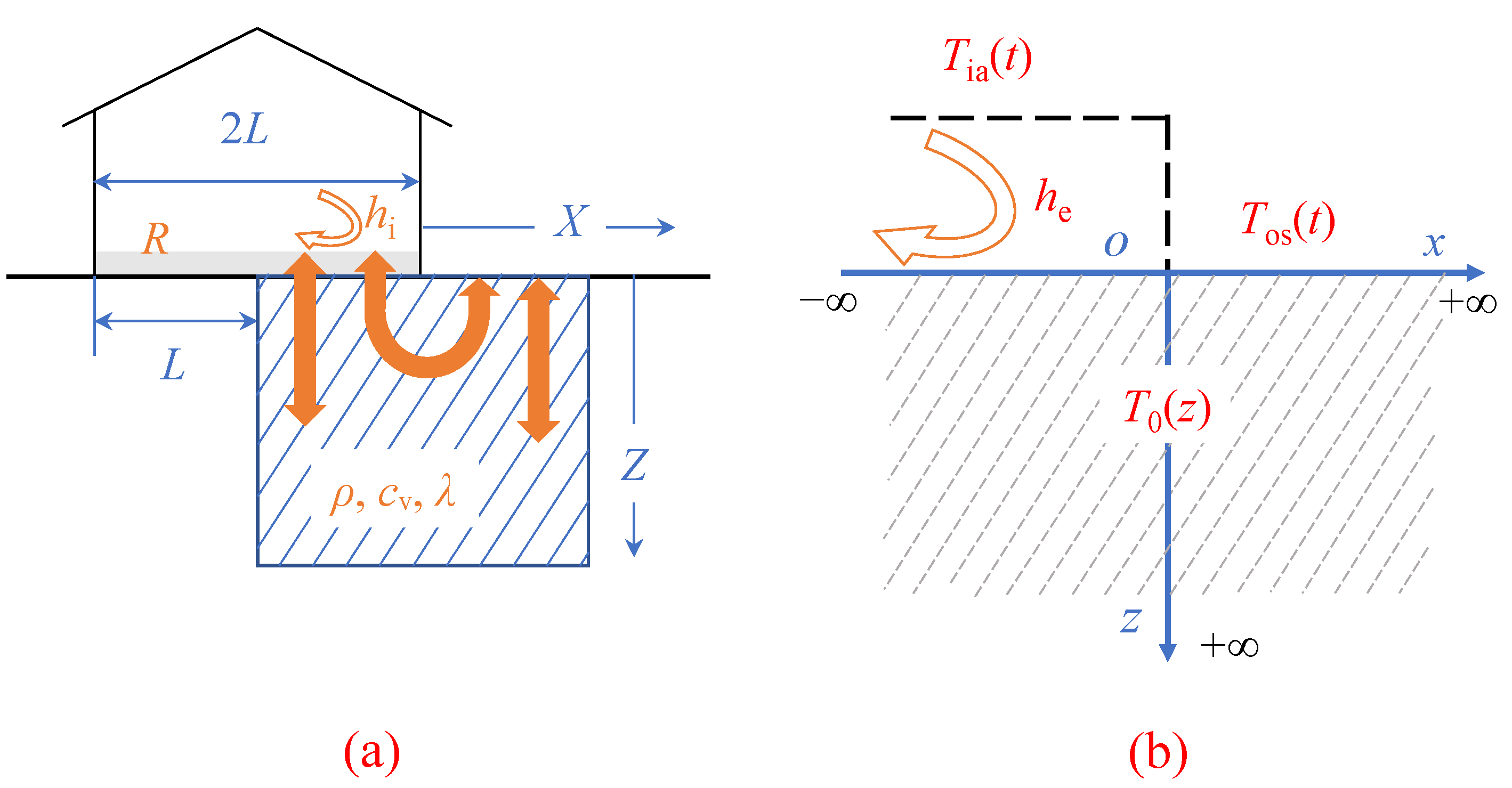
2.1. Heat Transfer Equation

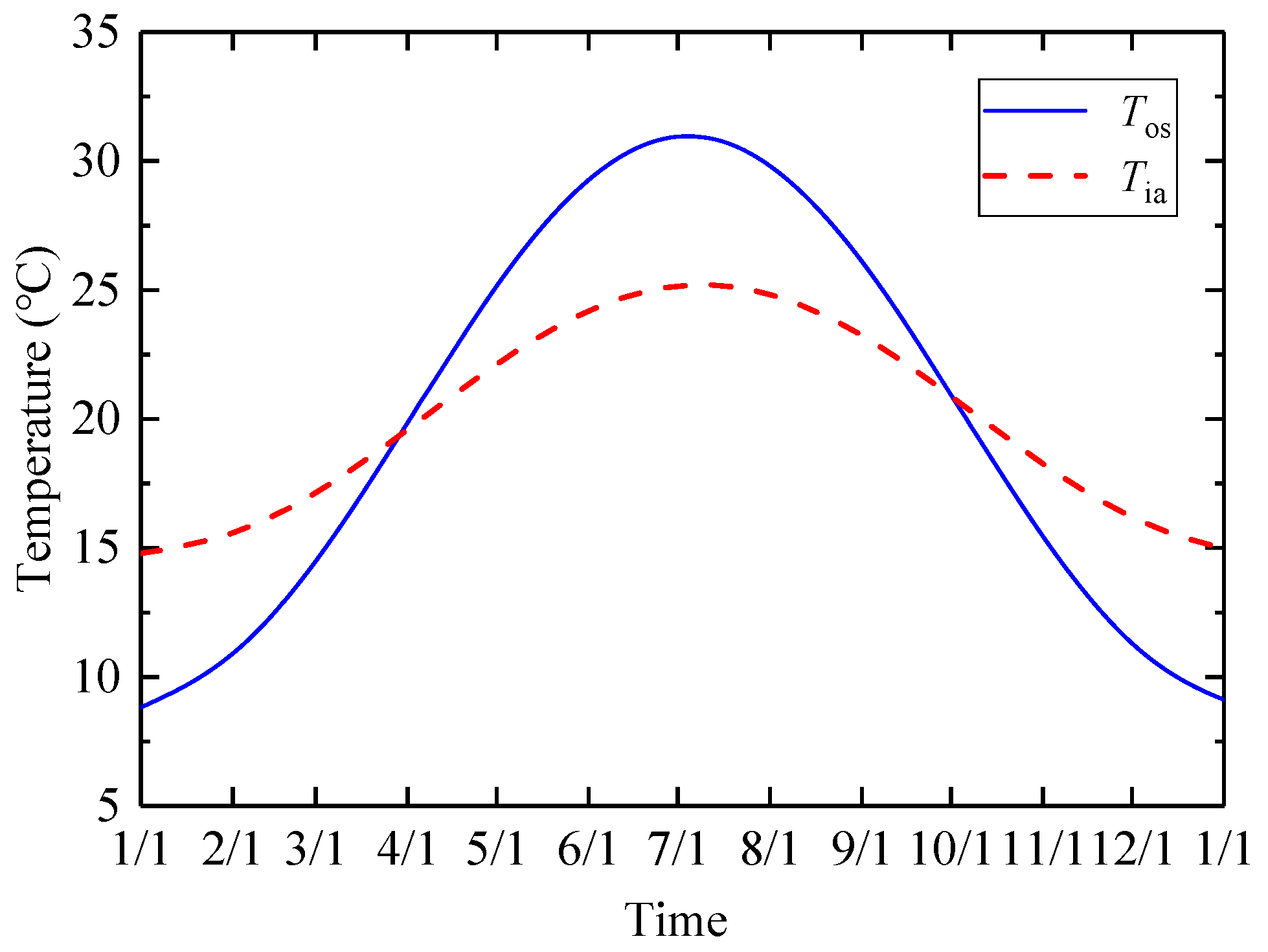
2.1.1. Temperature Boundaries

The heat balance of the ground surface includes the conduction with soil, the convection with air, and the radiation with the sun. In order to facilitate the study, the ground surface is treated as the Dirichlet boundary condition [30].

$$T_{\mathrm{os}}=T_{\mathrm{oa}}+\gamma I/h_{\mathrm{o}},$$

(1)

where $T_{\mathrm{os}}$ is outdoor ground surface temperature, °C; $T_{\mathrm{oa}}$ is the outdoor air temperature, °C; γ is the absorptivity of ground surface; I is the solar radiation intensity, W/m²; hₒ is outdoor convective heat transfer coefficient, W/(m²·K). Then it can be expanded into the Fourier series,

$$T_{\mathrm{os}}\left(t\right)=T_{\mathrm{om}}+{\displaystyle \sum _{n=1}^{\infty }\left(B_n\sin {\omega }_{n}t+C_n\cos {\omega }_{n}t\right)},$$

(2)

where $T_{\mathrm{om}}$ is annual mean temperature of outdoor air, °C; ω is angular frequency, rad/s; t is time, s.

The heat balance of the floor surface includes the conduction with the ground, the convection with indoor air, and the radiation with the interior surfaces of the walls. Moreover, sometimes, there might be insulation on the floor. Assuming the heat storage capacity of insulation is so small as to be negligible, the indoor surface convective coefficient could be equivalent to its heat resistance,

$$h_{\mathrm{e}}=1/\left(R+1/h_{\mathrm{i}}\right).$$

(3)

Here, hₑ is the equivalent convective coefficient, W/(m²·K); R is the heat resistance of insulation, m²·K/W; hᵢ is the floor surface convective coefficient, W/(m²·K). Thus, the floor surface is considered as the Robin boundary condition. Similarly, indoor air temperature can also be expanded into the Fourier series.

$$T_{\mathrm{ia}}\left(t\right)=T_{\mathrm{im}}+{\displaystyle \sum _{n=1}^{\infty }\left(D_n\sin {\omega }_{n}t+E_n\cos {\omega }_{n}t\right)},$$

(4)

where $T_{\mathrm{im}}$ is the annual mean temperature of indoor air, °C.

2.1.2. Governing Equation

As for the two-dimensional ground-coupled floor heat transfer in temporary housing, as shown in Figure 1, the governing equation is

$$\frac{\partial T\left(x,z,t\right)}{\partial t}=\alpha \cdot {\nabla }^{2}T\left(x,z,t\right).$$

(5)

Here, z is the depth of the soil, m, and positive denotes the downward direction vertical to the ground; α is soil heat diffusion coefficient, m²/s; $\nabla$ is the Laplace operator. α = λ/(ρ c_p), where λ is soil heat conductivity, W/(m·K); ρ is soil density, kg/m³; and c_p is soil specific heat capacity, J/(kg·K).

Indoor floor surface (x < 0) is considered as Robin condition, and outdoor ground surface (x > 0) is Dirichlet condition.

$$\{\begin{array}{l}T\left(x,0,t\right)-h^{*}\cdot \frac{\partial T\left(x,0,t\right)}{\partial z}=T_{\mathrm{ia}}\left(t\right), x<0;\hfill \\ T\left(x,0,t\right)=T_{\mathrm{os}}\left(t\right), x>0,\hfill \end{array}$$

(6)

where h* = λ/h. If the indoor floor is attached to insulation, the equivalent convective heat transfer coefficient can be calculated by Equation (3).

The initial condition is

$$T\left(x,z,0\right)=T_0\left(z\right).$$

(7)

$T_0\left(z\right)$ could be calculated by the one-dimensional soil heat transfer problem.

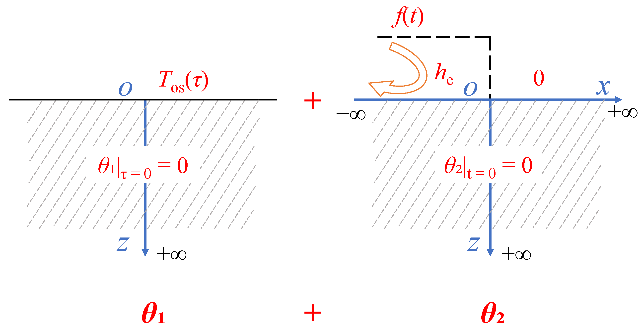
2.2. Superposition Principle

According to the superposition principle, as shown in Figure 2, the governing Equations (5)–(7) can be written as the sum of two equations. Suppose that T = θ₁ + θ₂, then

$$\{\begin{array}{l}\frac{\partial {\theta }_1\left(z,\tau \right)}{\partial \tau }=\alpha \cdot \frac{{\partial }^2{\theta }_1\left(z,\tau \right)}{\partial z^2};\hfill \\ {\theta }_1\left(0,\tau \right)=T_{\mathrm{os}}\left(\tau \right);\hfill \\ {\theta }_1\left(z,0\right)=0,\hfill \end{array}$$

(8)

and

$$\{\begin{array}{l}\frac{\partial {\theta }_2\left(x,z,t\right)}{\partial t}=\alpha \cdot {\nabla }^2{\theta }_2\left(x,z,t\right);\hfill \\ {\theta }_2\left(x,0,t\right)-h^{*}\cdot \frac{\partial {\theta }_2\left(x,0,t\right)}{\partial z}=f\left(t\right), x<0;\hfill \\ {\theta }_2\left(x,0,t\right)=0, x>0;\hfill \\ {\theta }_2\left(x,z,0\right)=0.\hfill \end{array}$$

(9)

$$f\left(t\right)=T_{\mathrm{ia}}\left(t\right)-T_{\mathrm{ea}}\left(t\right).$$

(10)

$$T_{\mathrm{ea}}\left(t\right)=T_{\mathrm{os}}\left(t\right)+q\left(t\right)\cdot h^{-1}.$$

(11)

The time τ counts before the building is constructed, while time t counts after that. The heat flux q(t) could be obtained by solving Equation (8).

Equation (8) describes the heat storage and release process of soil without building shelter, i.e., a classical one-dimensional semi-infinite solid heat transfer problem. When the boundary condition is Fourier series as Equation (2), and θ₁(x, z, t) → $T_{\mathrm{om}}$ at z → ∞, the steady periodic solution of soil temperature is [31],

$${\theta }_1\left(z,t\right)=T_{\mathrm{om}}+{\displaystyle \sum _{n=1}^N{e}^{-z/d_n}\cdot \left[B_n\sin \left({\omega }_{n}t-z/d_n\right)+C_n\cos \left({\omega }_{n}t-z/d_n\right)\right]},$$

(12)

$$d_n=\sqrt{2\alpha /{\omega }_n}.$$

(13)

The heat flux q(t) at z = 0 is

$$q\left(t\right)=\lambda \cdot {\displaystyle \sum _{n=1}^N{d}_n^{-1}\cdot \left[\left(B_n-C_n\right)\cdot \sin {\omega }_{n}t+\left(B_n+C_n\right)\cos {\omega }_{n}t\right]}.$$

(14)

2.3. Solution of Mixed Boundary Problem

For the convenience of solving governing Equation (9), t* = t/α is defined. Then applying the Fourier transform in space x and the Laplace transform in time t* to temperature θ₂(x, z, t*), respectively. It is obtained that [29],

$${\Theta }_2\left(p,z,s\right)={\displaystyle {\int }_0^{\infty }\left({\displaystyle {\int }_{-\infty }^{\infty }{\theta }_2\left(x,z,t^{\ast }\right)e^{-\mathrm{j}px}dx}\right)e^{-s{t}^{\ast }}d{t}^{\ast }},$$

(15)

where j² = −1. The boundary condition could be written as

$${\theta }_{\mathrm{BC}}\left(x,0,t^{*}\right)=f\left(t^{*}\right)\cdot H\left(-x\right).$$

(16)

H(−x) is the Heaviside step function. With the application of transforms, it becomes

$${\Theta }_{\mathrm{BC}}\left(p,0,s\right)=\left[\pi \delta \left(p\right)-\frac{1}{\mathrm{j}p}\right]\cdot F\left(s\right).$$

(17)

δ(p) is the Impulse function. F(s) is the Laplace transform result of f(t*).

According to the differentiation properties of integral transforms, governing Equation (9) could be reduced to a linear 2nd-order differential equation with constant coefficients. Supposing that θ₂(x, z, t) → 0 at z → ∞, the form of general solution is

$${\Theta }_2\left(p,z,s\right)={\Gamma }_2\left(p,s\right)\cdot e^{-z\sqrt{p^2+s}}.$$

(18)

By applying the Wiener–Hopf technique [32], it could be calculated that

$${\Gamma }_2\left(p,s\right)=\frac{{\Theta }_{\mathrm{BC}}\left(p,0,s\right)}{1+h^{*}\sqrt{s}}\cdot \sqrt{-\mathrm{j}\left(1+h^{*}\sqrt{s}\right)}\cdot \frac{K^{+}\left(p,s\right)}{K\left(p,s\right)}.$$

(19)

$$K\left(p,s\right)=1+h^{*}\cdot \sqrt{p^2+s}$$

(20)

is the kernel function. In addition,

$$K^{+}\left(p,s\right)=k^{+}\left(p,s\right)\cdot K_0^{+}\left(p,s\right),k^{+}\left(p,s\right)=\sqrt{h^{*}p+\mathrm{j}\left(1+h^{*}\sqrt{s}\right)}.$$

(21)

$$K_0^{+}\left(p,s\right)=\sqrt{K_0\left(p,s\right)}\cdot \exp \left[-\frac{1}{2\pi \mathrm{j}}\mathrm{P}.\mathrm{V}.{\displaystyle {\int }_{-\infty }^{\infty }\frac{\ln K_0\left(\xi ,s\right)}{\left(p-\xi \right)}d\xi }\right],$$

(22)

where P.V. denotes the Cauchy principal value integral.

$$K_0\left(p,s\right)=K\left(p,s\right)/k\left(p,s\right),k\left(p,s\right)=\sqrt{{\left(h^{*}p\right)}^2+{\left(1+h^{*}\sqrt{s}\right)}^2}.$$

(23)

2.4. Heat Fluxes Calculation

Heat fluxes through ground-coupled floors could be divided into two parts [5]. One part is the one-dimensional heat transfer along the z-axis, which is called the “face heat flux”. At enough distance away from walls, the heat transfer could be thought of as only one-dimensional. Another part is the heat transfer between the inside and outside environment near walls, which is called the “edge heat flux”. It is obtained by subtracting the face heat flux from the total heat flux.

3. Numerical Evaluation and Validation

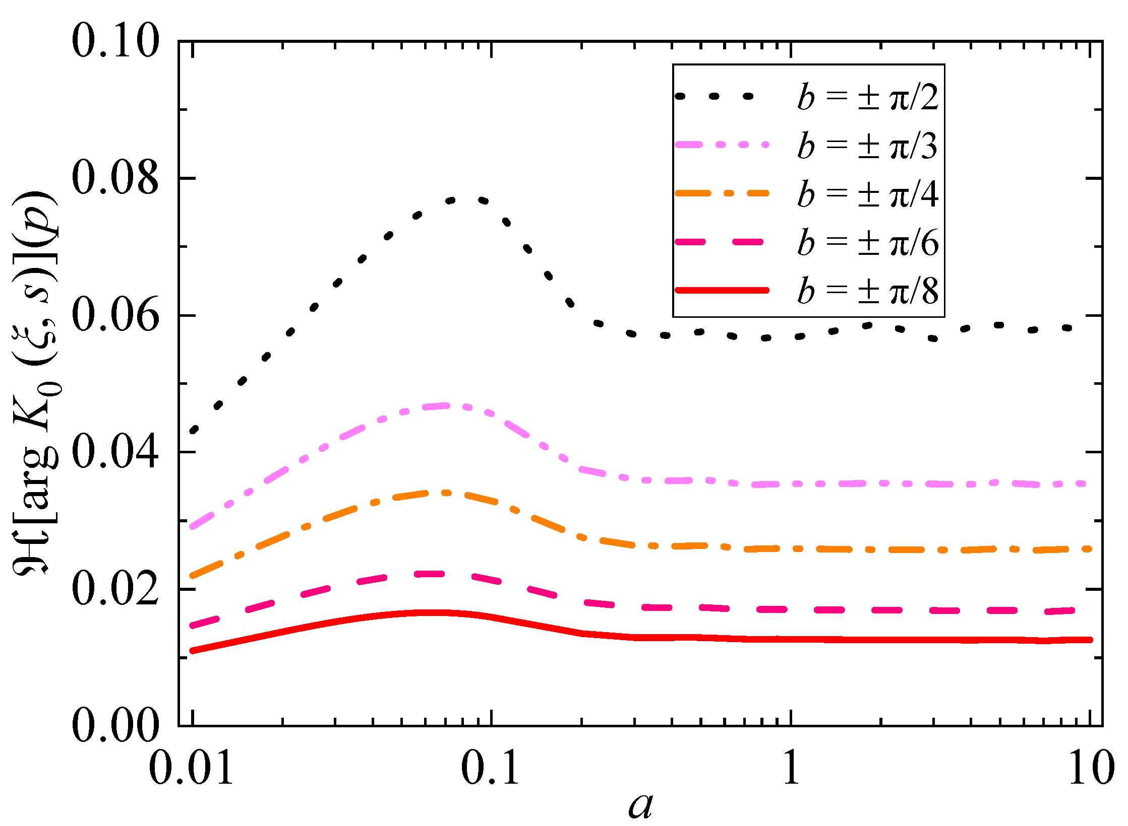
3.1. Numerical Evaluation of the Solution

Substitute Equation (19) into Equation (18), and then use the inverse Fourier transform and the inverse Laplace transform to obtain the temperature distribution θ₂(x, z, t) in Equation (9). However, to analytically calculate the inverse transforms is so difficult, even impossible. Thus, a numerical evaluation method is discussed.

Firstly, the fast Fourier transform (FFT) method could calculate the inverse Fourier transform efficiently. Noting that there is a singularity at p = 0. So

$${\Theta }_{\mathrm{BC}}\left(p,0,s\right)=-\frac{1}{\mathrm{j}p-\epsilon }\cdot F\left(s\right)$$

(24)

is used to replace Equation (17), where ε > 0 and ε → 0. Subtract and add the same term to the right-hand side of Equation (18) as [29]

$${\Theta }_2\left(p,z,s\right)={\Gamma }_2\left(p,s\right)\cdot e^{-z\sqrt{p^2+s}}-\frac{{\Theta }_{\mathrm{BC}}\left(p,0,s\right)}{1+h^{*}\sqrt{s}}\cdot e^{-z\cdot \left(\left|p\right|+\sqrt{s}\right)}+\frac{{\Theta }_{\mathrm{BC}}\left(p,0,s\right)}{1+h^{*}\sqrt{s}}\cdot e^{-z\cdot \left(\left|p\right|+\sqrt{s}\right)},$$

(25)

making sure that the sum of the first two terms on the right side is equal to 0 at p = 0. The remained third term could be analyzed separately, as

$$\frac{1}{2\pi }{\displaystyle {\int }_{-\infty }^{\infty }\frac{{\Theta }_{\mathrm{BC}}\left(p,0,s\right)}{1+h^{*}\sqrt{s}}\cdot e^{-z\cdot \left(\left|p\right|+\sqrt{s}\right)+\mathrm{j}xp}dp=}\frac{F\left(s\right)}{1+h^{*}\sqrt{s}}\cdot \left[\frac{1}{2}-\frac{1}{\pi }\cdot \arctan \left(\frac{x}{z}\right)\right]\cdot e^{-z\sqrt{s}}.$$

(26)

Secondly, since the complex logarithm of the complex function K₀(ξ, s) is that

$$\ln K_0\left(\xi ,s\right)=\ln \left|K_0\left(\xi ,s\right)\right|+\mathrm{j}\cdot \arg K_0\left(\xi ,s\right),$$

(27)

the integral in Equation (22) is divided into two terms

$$\frac{1}{\pi }\mathrm{P}.\mathrm{V}.{\displaystyle {\int }_{-\infty }^{\infty }\frac{\ln K_0\left(\xi ,s\right)}{\left(p-\xi \right)}d\xi }=\frac{1}{\pi }\cdot {\displaystyle {\int }_{-\infty }^{\infty }\frac{\ln \left|K_0\left(\xi ,s\right)\right|}{\left(p-\xi \right)}d\xi }+\frac{\mathrm{j}}{\pi }\cdot {\displaystyle {\int }_{-\infty }^{\infty }\frac{\arg K_0\left(\xi ,s\right)}{\left(p-\xi \right)}d\xi }.$$

(28)

These integrals in Equation (28) are known as the Hilbert transform, which also could be approximated based on the FFT algorithm [33]. The ℌ [.] denotes the Hilbert transform. As shown in Figure 3, the Hilbert transform of the argument function arg K₀(ξ, s) has an absolute maximum of under 0.08 when the argument of s belongs to (−π/2, π/2). Only half of the value of the Hilbert transform is the index of the exponential function in Equation (22). Even if it was treated as 0, the relative errors of results obtained are less than 5%. Thus, by ignoring the second term on the right-hand side of Equation (28), Equation (22) can be simplified to save computation time.

Finally, the convolution quadrature method [34] is applied to evaluate the inverse Laplace transform.

3.2. Validation

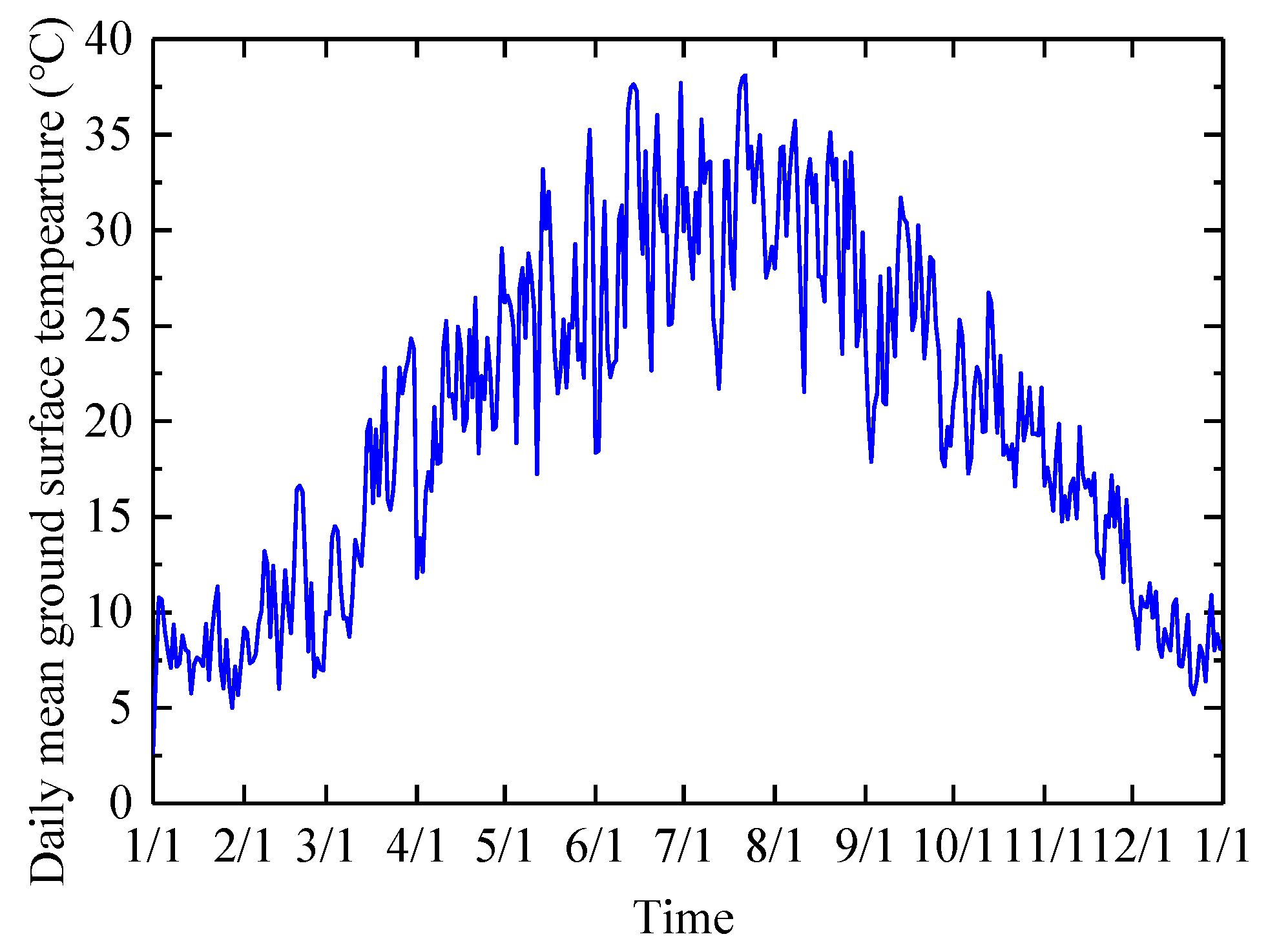
3.2.1. Temperature Boundaries

As shown in Figure 4, a case study of Chengdu city [35], the daily average outdoor ground surface temperatures were calculated by Equation (1). As shown in Figure 5, three terms of its Fourier series were picked.

$$T_{\mathrm{os}}=20.14+0.29\sin {\omega }_{1}t-11.33\cos {\omega }_{1}t,$$

(29)

where ω₁ = 2π/(8760 × 3600).

Then, an acceptable indoor thermal environment was assumed, e.g., indoor air temperatures were linearly correlated to outdoor air [20],

$$T_{\mathrm{ia}}=0.556T_{\mathrm{oa}}+10.9.$$

(30)

Similarly, three terms of its Fourier series were picked.

$$T_{\mathrm{ia}}=20.11-0.27\sin {\omega }_{1}t-5.31\cos {\omega }_{1}t.$$

(31)

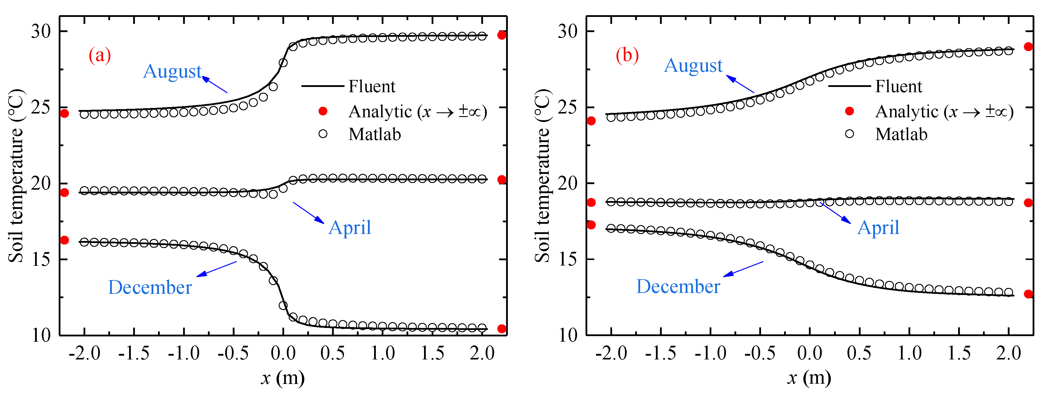
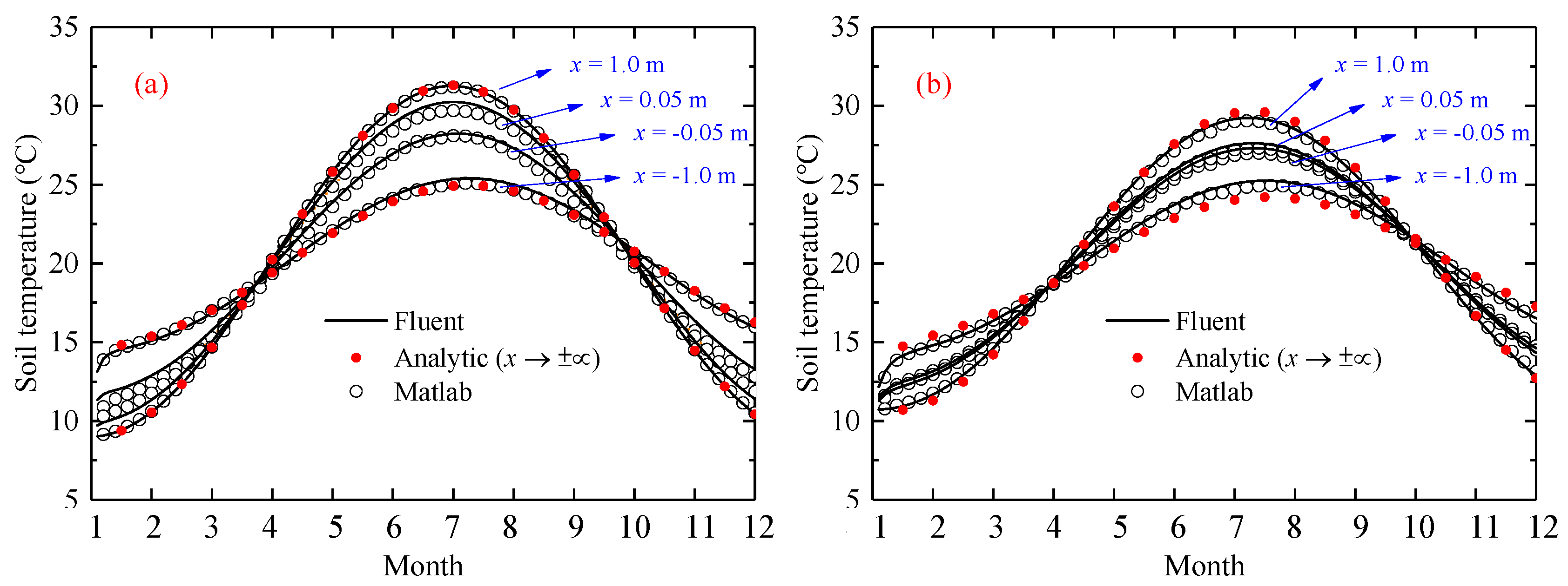
3.2.2. Comparison with Fluent Simulated Results

With the numerical evaluation method discussed above, the soil temperature could be easily calculated by the Matlab tool.

Table 1. Detailed thermophysical properties of ground-coupled floors [28,36].

Parameters	Units	Value	Parameters	Units	Value
Soil heat conductivity (λ)	W/(m·K)	2	Ground surface absorptivity (γ)	-	0.8
Soil density (ρ)	kg/m3	1500	Outdoor convective heat transfer coefficient (hₒ)	W/(m2·K)	23
Soil specific heat (cp)	J/(kg·K)	1350	Indoor convective heat transfer coefficient (hᵢ)	W/(m2·K)	8.7

lists the thermophysical properties of soil and ground surfaces. The temperatures in the range of −10 m ≤ x ≤ 10 m were calculated. The step size was Δx = 0.05 m, and the time step size was Δt = 86,400 s. The Ansys Fluent software based on the finite volume method was utilized to validate the accuracy of the analytical solution and its numerical evaluation. A two-dimensional rectangular physical model was established, as diagonal stripes filled the region in Figure 1. Detailed sizes were that the indoor floor length was L = 5 m, the outdoor ground length was X = 5 m, and the soil depth was Z = 5 m. Then, regular mesh with step sizes of 0.1 m on both horizontal and vertical directions, as well as time step size Δt = 259,200 s, were chosen.

Figure 6 and Figure 7 described, respectively, the soil temperature distribution along the x dimension and the temperature variation over time. At x → +∞, the soil heat conduction could be thought of as one-dimensional in Equation (8). Its temperature distribution along the z-axis was calculated by Equation (12), which was marked with solid red circles in the figures. While, at x → −∞, the soil temperature also conformed to a one-dimensional heat transfer model. Carslaw and Jaeger analyzed it and obtained the solution in the integral form [37], which was calculated and marked with solid red circles as well.

As shown in Figure 6, both at a soil depth of z = 0.05 m and z = 0.55 m, the numerical temperature results calculated by Matlab were in accord with the data simulated by Fluent. At the same time, for three time points (April, August, and December), their temperature trends, both in the positive and negative direction, were close to the exact solutions (red circle marks). It is worth mentioning that the FVM computation by Fluent took about several minutes, and the current method spent about several seconds. Therefore, it proved that the analytical solution evaluated numerically was accurate and efficient.

Figure 7 shows the soil temperatures varied with time at eight points (−1.0, 0.05), (−0.05, 0.05), (0.05, 0.05), (1.0, 0.05), (−1.0, 0.55), (−0.05, 0.55), (0.05, 0.55), and (1.0, 0.55). As was seen in the figure, the calculated temperatures by Matlab agreed well with the data by Fluent. It also could be found that the temperatures at x = 1.0 m and x = −1.0 m were closed to the exact solutions (red circle marks), which meant that the heat of the indoor floor and outdoor ground exchanged mainly around walls within the range of 1 m. Thus, calculating the heat transfer of the ground-coupled floor in temporary buildings by the current method was reliable.

4. Results and Discussion

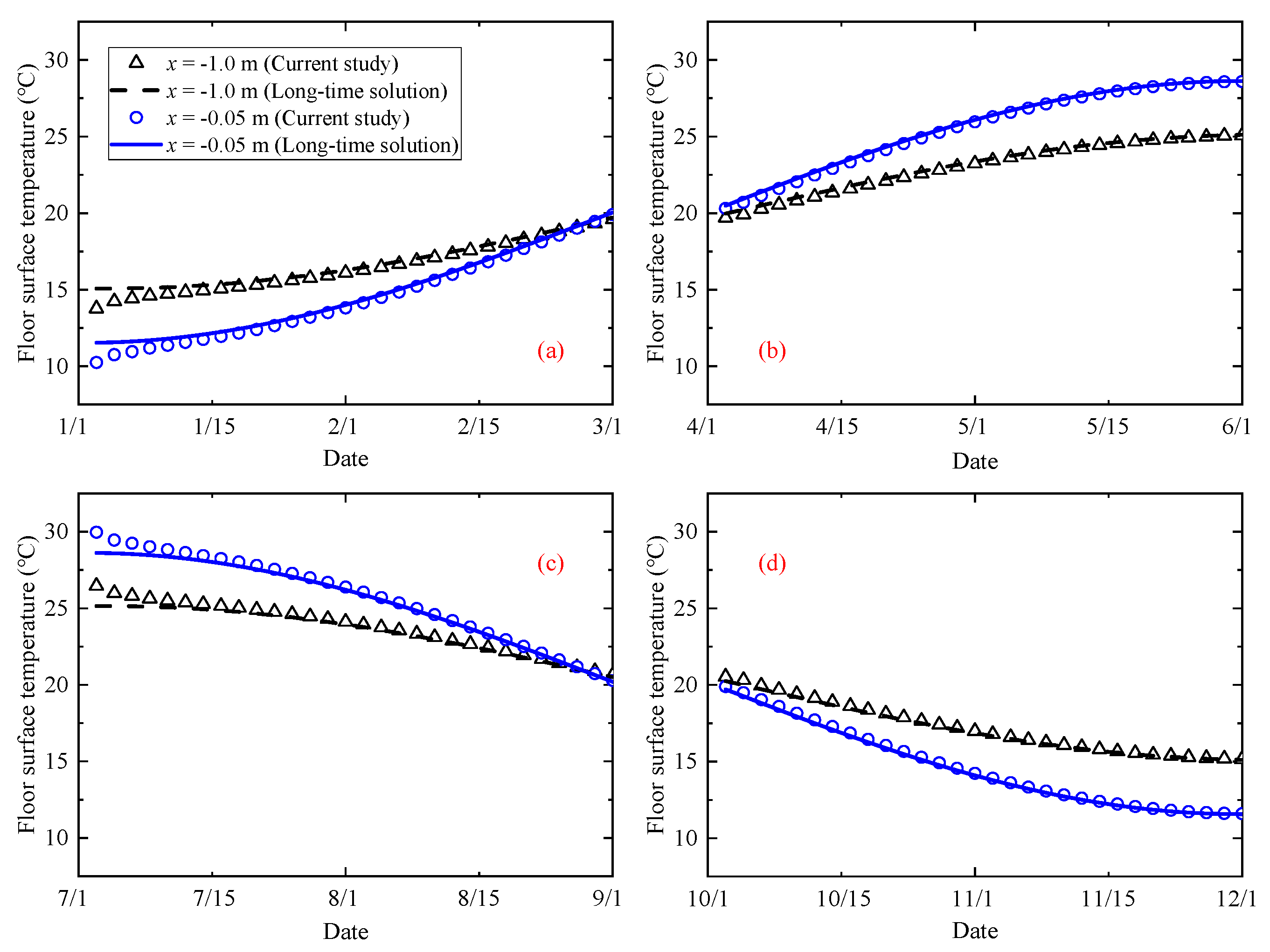
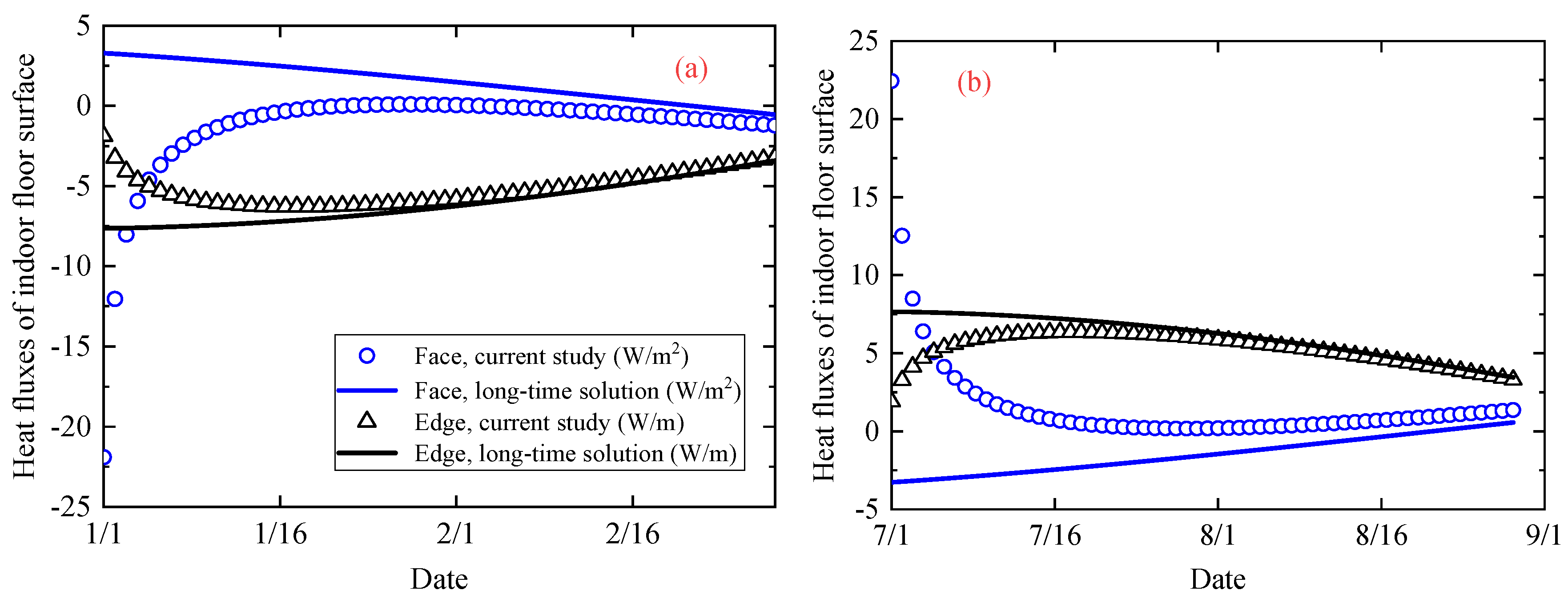
4.1. Differences with Long-Time Solutions

The long-time solutions of ground-couple heat transfer were developed mostly in previous studies, which ignored the initial temperature of the soil. In the current study, the initial conditions were also considered. The temperature at two positions of x = −0.05 m and x = −1.0 m were picked to represent the floor temperature distribution. Referring to Figure 6a, floor surface temperature had almost uniformly distributed in space, except for a small distance near walls (x = 0). Figure 8 shows the floor surface temperature in temporary housing built at different seasons. When buildings were built in the cold season, for example, on 1 January (Figure 8a), floor temperatures at the initial stage were lower than the long-time solution. In contrast, when buildings were built in the hot season, e.g., on 1 July (Figure 8c), the long-time solution underestimated the floor temperature at the initial stage. A visible temperature difference between the two solutions occurred if buildings were built in hot summer and cold winter. However, no obvious difference was found if temporary housing was built in transition seasons, seen in Figure 8b,d.

Figure 9 compares the floor surface heat fluxes between the current calculation and the long-time solution. Set 1 January and 1 July as examples of the cold and hot climates, respectively. Heat fluxes transferred into the indoor environment were defined as positive. It showed that there were obvious differences in the face and edge heat fluxes. Edge heat fluxes along with the wall were overestimated by the long-time solution both in cold and hot conditions. Moreover, the face heat fluxes of the two methods are directed in opposite directions.

Long-time solutions to ground-coupled heat conduction have been commonly investigated over the past several decades. Firstly, the initial transient was unimportant for air-conditioning calculation in conventional buildings. Secondly, it is quite difficult to solve the three-dimensional transient equations analytically. Nonetheless, some researchers have discussed the influence of initial soil conditions [38]. Luo et al. [39] found that more than 200 h of indoor temperature data had been significantly affected by the initial soil temperature conditions. Lachenbruch’s calculation showed that it took more than three years before ground-coupled heat transfer reached a steady annual periodic cycle for a rectangular slab of 100 ft × 30 ft [23,40]. The finding of this study was closer to Luo’s result. Given that a bigger slab size was calculated by Lachenbruch, it could be deduced that larger ground thermal storage capacities could result in bigger calculation differences. Moreover, floor insulation and extreme outside temperature conditions did matter.

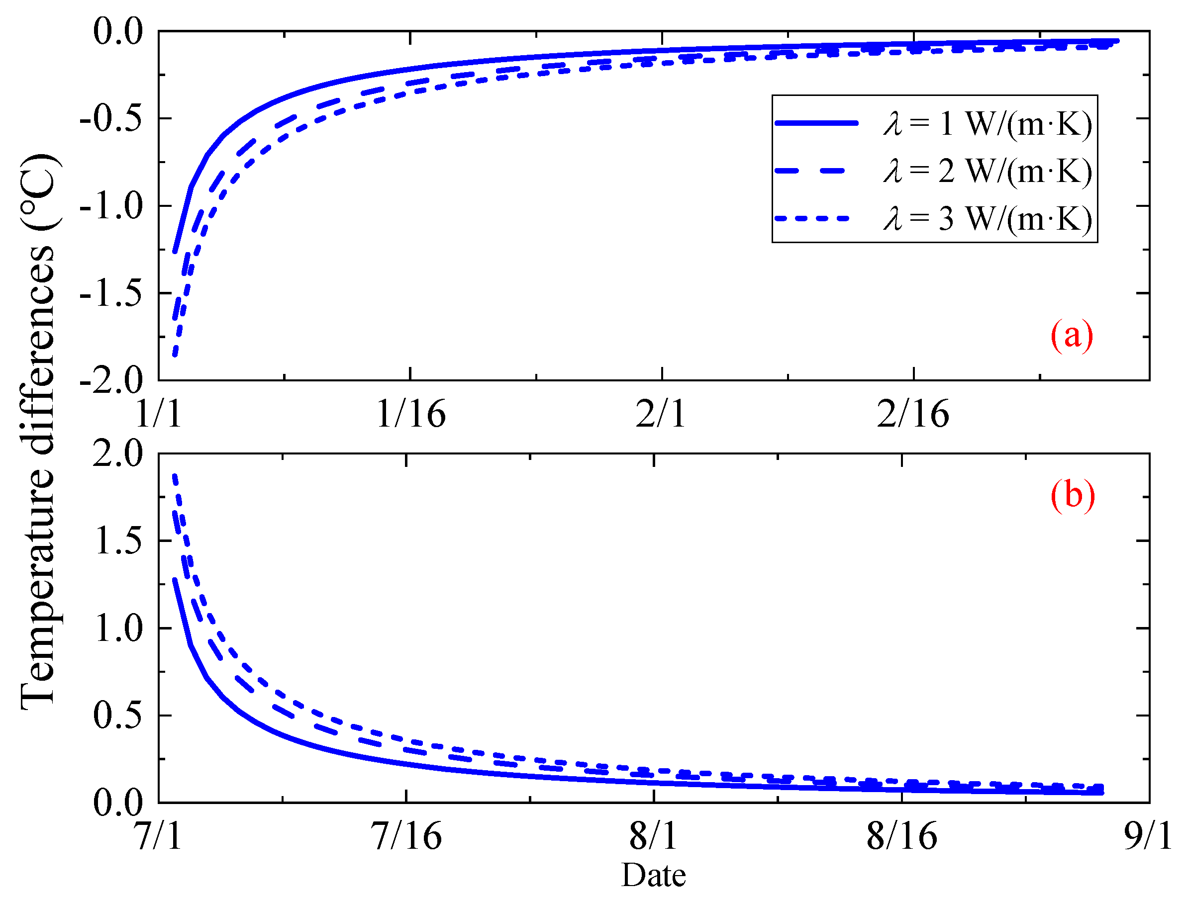
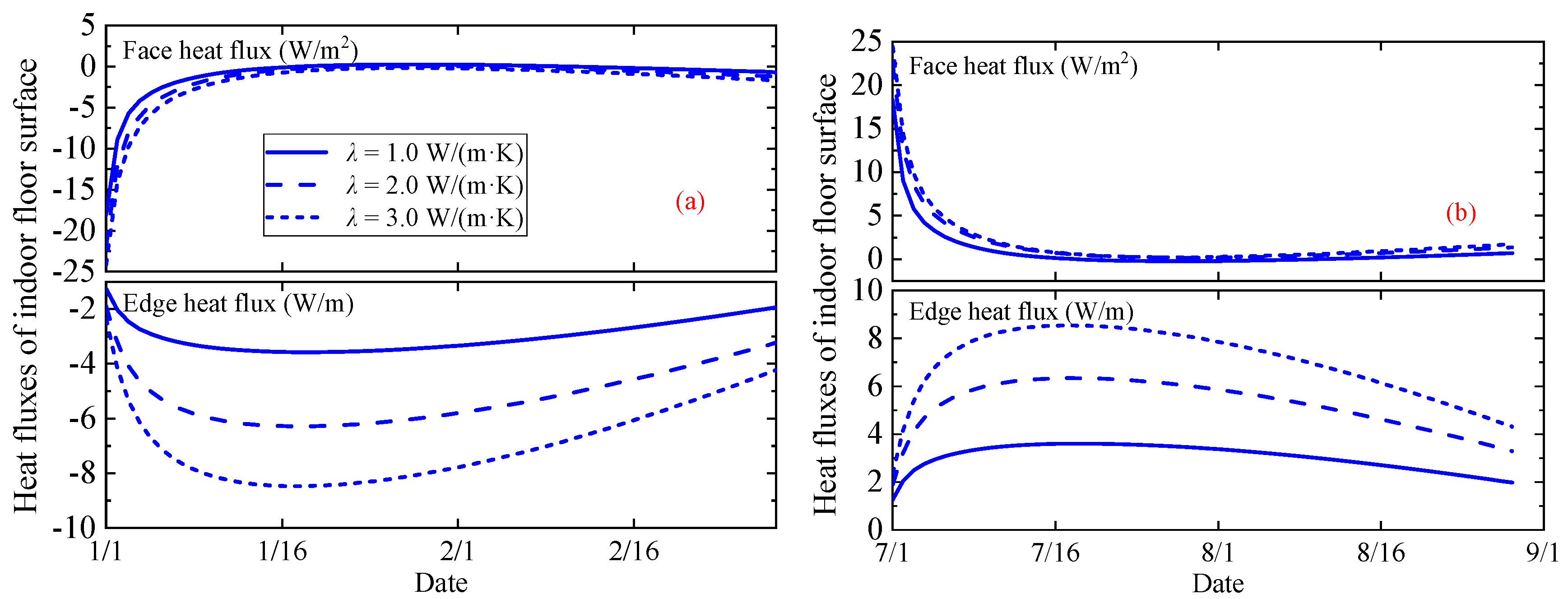
4.2. Effects of Soil Heat Conductivity

The higher the heat transfer capacity of the soil, the more heat or cold is stored in it. Figure 10 exhibited the floor surface temperature differences between the current study and the long-time solution at x = −1.0 m. Enough distance away from walls could lower the influence of the outdoor environment. It could be seen that temperature differences increased with the heat conductivity of the soil.

As shown in Figure 11, the face heat flux of the ground-couple floor was negative for temporary housing built in cold climates and was positive when built in hot climates. With the increase in soil heat conductivity, the absolute value of face heat flux increased. So did the edge heat flux.

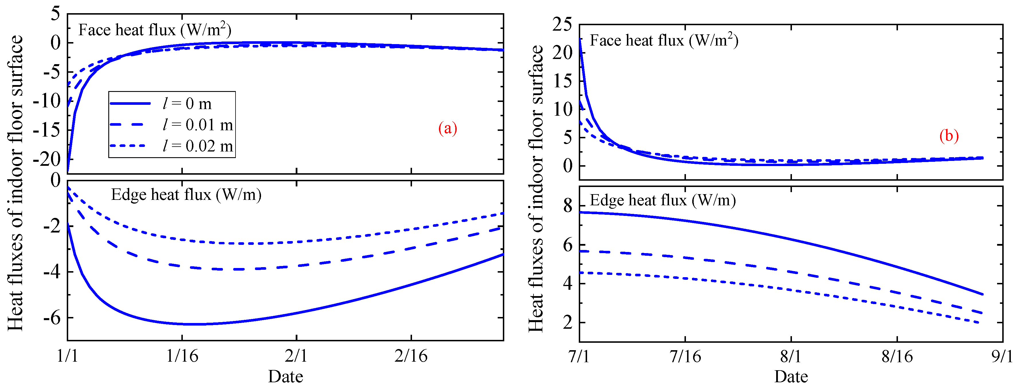
4.3. Effects of Floor Insulation

The expanded polystyrene (EPS) foam with heat conductivity of 0.042 W/(m·K) was assumed as floor insulation to study its effects on the floor surface heat flux. As shown in Figure 12, EPS insulation could obviously reduce both the face and the edge heat fluxes. The floor insulation could effectively decrease the heat transfer near walls, as 0.01 m and 0.02 m insulation could averagely reduce about 27% and 40% of the edge heat fluxes. As for face heat fluxes, the floor insulation resulted in a reduction at first and an increase then. The opposite direction of heat flux occurred in cold and hot climates. That is, the floor insulation just slowed down rather than prevented the cold or heat release of the ground.

5. Conclusions

Ground-coupled heat transfer calculation is an important and difficult issue in building simulation and air-conditioning design. A new semi-analytical calculation method was presented, in the current study, based on a two-dimensional transient heat transfer equation. Compared with the long-time solutions in previous studies, the new method could also calculate the initial transient heat transfer. Prior to this, numerical simulation methods are almost the only way to solve the initial transient ground-coupled issue. The current method is significant for temporary housing that is built rapidly and is of a short life cycle. At the same time, the method is more efficient than common numerical methods due to no iterative process.

The large influence of soil initial temperature conditions occurs in hot and cold climates when the indoor environment is exactly a concern. A more accurate calculation would be provided by the current method, while long-time solutions might even misestimate heat flux directions. It was concluded that larger ground thermal capacity would have more effects on the initial heat transfer of ground-coupled floor. That is, thermophysical parameters of ground, such as the density, the heat conductivity, and the specific heat capacity, are of significance. Moreover, insulation could effectively reduce the heat exchange between indoor and outdoor environments and slow down the thermal release of ground.

The same as other analytical solutions, the current method is not able to deal with complex floor configuration problems. In addition, the coupled calculation of floor and building envelope heat transfer would be furtherly studied in future work, and helpful guidance could be provided for the air-conditioning design and energy demand prediction in temporary housing.

References

1. Chen, D. Dynamic three-dimensional heat transfer calculation for uninsulated slab-on-ground constructions. Energy Build. 2013, 60, 420–428. [Google Scholar] [CrossRef]
2. Neymark, J.; Judkoff, R.; Beausoleil-Morrison, I.; Ben-Nakhi, A.; Crowley, M.; Deru, M.; Henninger, R.; Ribberink, H.; Thornton, J.; Wijsman, A.; et al. International Energy Agency Building Energy Simulation Test and Diagnostic Method (IEA BESTEST): In-Depth Diagnostic Cases for Ground Coupled Heat Transfer Related to Slab-on-Grade Construction; NREL/TP-550-43388; National Renewable Energy Laboratory: Golden, CO, USA, 2008. [CrossRef] [Green Version]
3. Zoras, S. A Review of Building Earth-Contact Heat Transfer. Adv. Build. Energy Res. 2009, 3, 289–313. [Google Scholar] [CrossRef]
4. Ren, Z.; Motlagh, O.; Chen, D. A correlation-based model for building ground-coupled heat loss calculation using Artificial Neural Network techniques. J. Build. Perform. Simul. 2020, 13, 48–58. [Google Scholar] [CrossRef]
5. ASHRAE. Handbook, Fundamentals; American Society of Heating, Refrigerating and Air-Conditioning Engineers, Inc.: Peachtree Corners, GA, USA, 2009. [Google Scholar]
6. ISO 13370:2017; Thermal Performance of Buildings—Heat Transfer via The Ground—Calculation Methods. International Organization for Standardization: Geneva, Switzerland, 2017.
7. Andolsun, S.; Culp, C.H.; Haberl, J.S.; Witte, M.J. EnergyPlus vs. DOE-2.1e: The effect of ground coupling on cooling/heating energy requirements of slab-on-grade code houses in four climates of the US. Energy Build. 2012, 52, 189–206. [Google Scholar] [CrossRef]
8. Delsante, A.; Stokes, A.; Walsh, P. Application of Fourier transforms to periodic heat flow into the ground under a building. Int. J. Heat Mass Transf. 1983, 26, 121–132. [Google Scholar] [CrossRef]
9. Delsante, A. Theoretical calculations of the steady-state heat losses through a slab-on-ground floor. Build. Environ. 1988, 23, 11–17. [Google Scholar] [CrossRef]
10. Davies, M. Heat loss from a solid ground floor. Build. Environ. 1993, 28, 347–359. [Google Scholar] [CrossRef]
11. Richards, P.; Mathews, E. A thermal design tool for buildings in ground contact. Build. Environ. 1994, 29, 73–82. [Google Scholar] [CrossRef]
12. Bahnfleth, W.P. Three Dimensional Modeling of Heat Transfer from Slab Floors. Ph.D. Thesis, University of Illinois, Urbana, IL, USA, 1989. [Google Scholar]
13. Stephson, D.G.; Mitalas, G.P. Cooling load calculations by thermal response factor method. ASHRAE Trans. Part 1 1967, 73, III.2.1.–III.2.10. [Google Scholar]
14. Stephson, D.G.; Mitalas, G.P. Calculation of heat conduction transfer functions for multi-layer slabs. ASHRAE Trans. Part II 1971, 77, 117–126. [Google Scholar]
15. Ceylan, H.T.; Myers, G.E. Long-Time Solutions to Heat-Conduction Transients with Time-Dependent Inputs. J. Heat Transf. 1980, 102, 115–120. [Google Scholar] [CrossRef]
16. Zhong, Z.; Braun, J.E. A simple method for estimating transient heat transfer in slab-on-ground floors. Build. Environ. 2007, 42, 1071–1080. [Google Scholar] [CrossRef]
17. Baladés, J.D.M.; Maestre, I.R.; Gómez, P.; Blázquez, J.L.F. Applicability of One-Dimensional Transient Solutions for Ground-Coupled Heat Transfer in Buildings. Appl. Mech. Mater. 2013, 361, 386–390. [Google Scholar] [CrossRef]
18. Manoochehry, S.; Hoseinzadeh, E.; Taha, P.; Rasouli, H.R.; Hoseinzadeh, S. Field Hospital in Disasters: A Systematic Review. Trauma Mon. 2019, 24, 9. [Google Scholar] [CrossRef]
19. Wang, Y.; Wang, L.; Long, E.; Deng, S. An experimental study on the indoor thermal environment in prefabricated houses in the subtropics. Energy Build. 2016, 127, 529–539. [Google Scholar] [CrossRef]
20. Thapa, R.; Rijal, H.B.; Shukuya, M. Field study on acceptable indoor temperature in temporary shelters built in Nepal after massive earthquake 2015. Build. Environ. 2018, 135, 330–343. [Google Scholar] [CrossRef]
21. Poschl, R. Modelling the Thermal Comfort Performance of Tents Used In Humanitarian Relief. Ph.D. Thesis, Loughborough University, Loughborough, UK, 2017. [Google Scholar]
22. Yan, S.-R.; Fazilati, M.A.; Samani, N.; Ghasemi, H.R.; Toghraie, D.; Nguyen, Q.; Karimipour, A. Energy efficiency optimization of the waste heat recovery system with embedded phase change materials in greenhouses: A thermo-economic-environmental study. J. Energy Storage 2020, 30, 101445. [Google Scholar] [CrossRef]
23. Lachenbruch, A.H. Three-Dimensional Heat Conduction in Permafrost Beneath Heated Buildings; U.S. Government Printing Office: Washington, DC, USA, 1957. [CrossRef] [Green Version]
24. Cornaro, C.; Sapori, D.; Bucci, F.; Pierro, M.; Giammanco, C. Thermal performance analysis of an emergency shelter using dynamic building simulation. Energy Build. 2015, 88, 122–134. [Google Scholar] [CrossRef]
25. Crawford, C.; Manfield, P.; McRobie, A. Assessing the thermal performance of an emergency shelter system. Energy Build. 2005, 37, 471–483. [Google Scholar] [CrossRef]
26. Obyn, S.; van Moeseke, G.; Virgo, V. Thermal performance of shelter modelling: Improvement of temporary structures. Energy Build. 2015, 89, 170–182. [Google Scholar] [CrossRef]
27. Wang, C.; Deng, S.; Niu, J.; Long, E. A numerical study on optimizing the designs of applying PCMs to a disaster-relief prefabricated temporary-house (PTH) to improve its summer daytime indoor thermal environment. Energy 2019, 181, 239–249. [Google Scholar] [CrossRef]
28. Liu, F.; Yan, L.; Meng, X.; Zhang, C. A review on indoor green plants employed to improve indoor environment. J. Build. Eng. 2022, 53, 104542. [Google Scholar] [CrossRef]
29. Gorbushin, N.; Nguyen, V.-H.; Parnell, W.J.; Assier, R.C.; Naili, S. Transient thermal boundary value problems in the half-space with mixed convective boundary conditions. J. Eng. Math. 2019, 114, 141–158. [Google Scholar] [CrossRef] [Green Version]
30. Adjali, M.; Davies, M.; Rees, S.; Littler, J. Temperatures in and under a slab-on-ground floor: Two- and three-dimensional numerical simulations and comparison with experimental data. Build. Environ. 2000, 35, 655–662. [Google Scholar] [CrossRef]
31. Badache, M.; Eslami-Nejad, P.; Ouzzane, M.; Aidoun, Z.; Lamarche, L. A new modeling approach for improved ground temperature profile determination. Renew. Energy 2016, 85, 436–444. [Google Scholar] [CrossRef]
32. Parnell, W.J.; Nguyen, V.-H.; Assier, R.; Naili, S.; Abrahams, I.D. Transient Thermal Mixed Boundary Value Problems in the Half-Space. SIAM J. Appl. Math. 2016, 76, 845–866. [Google Scholar] [CrossRef] [Green Version]
33. MathWorks. Available online: https://ww2.mathworks.cn/help/signal/ref/hilbert.html?s_tid=srchtitle#d120e72684 (accessed on 30 October 2022).
34. Schanz, M.; Antes, H. Application of ‘Operational Quadrature Methods’ in Time Domain Boundary Element Methods. Meccanica 1997, 32, 179–186. [Google Scholar] [CrossRef]
35. EnergyPlus. Available online: https://www.energyplus.net/weather-location/asia_wmo_region_2/CHN/CHN_Sichuan.Chengdu.562940_CSWD (accessed on 30 October 2022).
36. GB 50176-2016; Code for Thermal Design of Civil Building. China Architecture & Building Press: Beijing, China, 2016.
37. Carslaw, H.S.; Jaeger, J.C. Conduction of Heat in Solids; Clarendon Press: Oxford, UK, 1959; Chapter 14.2; p. 350. [Google Scholar]
38. Hagentoft, C.E. Heat Loss to The Ground from a Building: Slab on The Ground and Cellar; Report TVBH-1004; Lund Institute of Technology: Lund, Sweden, 1988. [Google Scholar]
39. Luo, C.; Moghtaderi, B.; Page, A. Effect of ground boundary and initial conditions on the thermal performance of buildings. Appl. Therm. Eng. 2010, 30, 2602–2609. [Google Scholar] [CrossRef]
40. Kusuda, T.; Mizuno, M.; Bean, J.W. Seasonal Heat Loss Calculation for Slab-On-Grade Floors; NBSIR 81-2420; National Bureau of Standards, Center for Building Technology, Building Physics Division: Washington, DC, USA, 1982.
Figure 1. Ground-couple floor model of: (a) heat transfer; (b) semi-infinite solid.
Applsci 12 11844 g001
Figure 2. Linear decomposition of ground-coupled floor heat transfer equation.
Applsci 12 11844 g002
Figure 3. Hilbert transform of arg K0(ξ, s) at different s (s = a·eᵇʲ), when h* belongs to (0.01, 10).
Applsci 12 11844 g003
Figure 4. Daily mean ground surface temperature in Chengdu.
Applsci 12 11844 g004
Figure 5. Outdoor ground surface temperatures and indoor air temperatures.
Applsci 12 11844 g005
Figure 6. Soil temperature distribution along x dimension at (a) z = 0.05 m; (b) z = 0.55 m.
Applsci 12 11844 g006
Figure 7. Soil temperature variation over time at (a) z = 0.05 m; (b) z = 0.55 m.
Applsci 12 11844 g007
Figure 8. Floor temperatures in temporary housing built (a) on 1 January; (b) on 1 April; (c) on 1 July; (d) on 1 October.
Applsci 12 11844 g008
Figure 9. Indoor floor surface heat fluxes in temporary housing built (a) on 1 January; (b) on 1 July.
Applsci 12 11844 g009
Figure 10. Calculated floor surface temperature differences with a long-time solution at x = −1.0 m for new buildings built (a) on 1 January; (b) on 1 July.
Applsci 12 11844 g010
Figure 11. Ground-coupled heat fluxes in temporary housing built (a) on 1 January; (b) on 1 July.
Applsci 12 11844 g011
Figure 12. Effects of floor insulation on the face and edge heat fluxes of floor surface in temporary housing built (a) on 1 January; (b) on 1 July.
Applsci 12 11844 g012