A Mathematical Model for Bioremediation of Hydrocarbon-Contaminated Soils

Featured Application

The developed mathematical model can be used as a decision-supporting tool for the definition of the best strategies for in situ bioremediation of contaminated sites.

Abstract

Bioremediation of hydrocarbons in soil is a highly complex process, involving a multiplicity of physical, chemical and biological phenomena. Therefore, it is extremely difficult to control and boost the bioremediation of these systems after an oil spill. A mathematical model was developed to assist in the prediction and decision-making regarding the in situ bioremediation of hydrocarbon-contaminated soils. The model considered the most relevant processes involved in the mass transfer and biodegradation of alkanes over time and along the depth of a flooded soil column. Aliphatic hydrocarbons were chosen since they are less water soluble than aromatics and account for 50–90% of the hydrocarbon fraction in several petroleum products. The effect of adding oxygen, nitrate, iron (III) or sulfate as electron acceptors was then simulated (bioremediation scenarios). Additionally, and to feed the model, batch assays were performed to obtain experimental data on hydrocarbon adsorption to soil particles (more than 60% of hydrocarbons tends to be adsorbed to soil particles), as well as hydrocarbon biodegradation rates in the presence of nitrate (0.114 d⁻¹) and oxygen (0.587 d⁻¹). The model indicates that saturated hydrocarbon removal occurs mainly with adsorption/desorption and transport processes in the upper layers of soil due to methanogenic biodegradation in deeper layers, since the other microbial processes are soon limited by the lack of electron acceptors. Simulation results show that higher initial electron acceptor concentrations led to higher hydrocarbon removal, confirming that the model is performing in accordance with the expected. Close to the surface (at 0.1 m depth), all scenarios predicted more than 83% hydrocarbon removal after two years of simulation. Soil re-aeration results in faster hydrocarbon removal (more than 20% after one year) and surfactants addition (around 15% after one year) may also accelerate soil bioremediation. With this model, the simultaneous contributions of the various physicochemical and biological processes are integrated, facilitating the simulation and comparison of different bioremediation scenarios. Therefore, it represents a useful support tool for the management of contaminated sites.

1. Introduction

Soil contamination constitutes a severe environmental problem. It is estimated to affect around 2.8 million sites in Europe [1], where mineral oils account for 22–24% of all the soil contamination incidents reported, and comprise 45% when considered together with BTEX and polyaromatic hydrocarbons [2]. The pollution of soils by petroleum hydrocarbons leads to ecological and health risks, due to their relatively low mobility and their toxic, mutagenic and carcinogenic effects [3,4].

The fate of petroleum hydrocarbons in soil is influenced by the physical and chemical properties of these compounds (e.g., solubility in water and affinity for the organic carbon in soil) as well as by the characteristics of the soil, such as particle size, porosity, organic matter content, permeability and surface area [3,5]. In general, soil acts as a sink for pollutants; thus, active cleaning operations must be performed to enable the recovery of contaminated soils within an acceptable timeframe [1].

To date, several physical and chemical remediation technologies are available (e.g., physical removal, soil washing and oxidation/reduction via chemical agents) [5,6]; however, there is an increasing willingness for the use of less aggressive and more eco-friendly techniques, such as bioremediation [7,8]. Critical factors in bioremediation are the availability of nutrients and electron acceptors (oxygen, nitrate, iron (III), sulfate) as well as the existence of microbial catabolic activity towards hydrocarbons [3,9,10]. Bioavailability of the contaminants also influences microbial activity, since the access of the microorganisms or their enzymes to the compounds can be hampered due to hydrocarbon interactions with the organic carbon content of the soil [3]. These aspects are particularly important when hydrocarbon contamination occurs in depth; for example, due to leaking underground storage tanks or pipelines. In permeable soils, the plume can penetrate to a significant depth, hindering the contamination removal and site decontamination [11].

Current knowledge of hydrocarbon biodegradation in soils is limited and requires further research. In addition, the selection and implementation of bioremediation approaches, as well as the prediction of the process outcomes, is highly complex. In this framework, mathematical modelling emerges as a promising tool, providing support for decision makers to effectively deal with the complexity of cleaning and restoring contaminated sites [12,13]. Over the years, mathematical modelling of hydrocarbon bioremediation has been performed, focused mainly on contaminated aquifers considering that relatively soluble hydrocarbon fractions will be transported from the contaminated soils to the water level, where further transport and biodegradation will occur [14,15,16]. Straight chain alkanes are less water soluble than other aliphatic and aromatic hydrocarbons and present a higher affinity for the organic carbon content of the soil. Moreover, saturated hydrocarbons account for 50–90% of the hydrocarbon fraction in several petroleum products (e.g., aviation gasoline, jet fuel, diesel fuel) [17]. As such, sequestration of this less soluble fraction of oil may occur in soils; its environmental fate is still not sufficiently studied. In soils, the majority of the developed models are designed for ex situ bioremediation [14,18,19,20]. In addition, only a few mathematical models couple mass transfer with Monod or first-order kinetics for hydrocarbon biodegradation [16,19,21,22,23], especially for less soluble hydrocarbons [16].

The aim of the present work was to develop a simple mathematical model to understand the processes involved in the decontamination of a saturated (flooded) soil column after an oil spill. This model can be used as a decision-supporting tool for the definition of the best strategies for in situ bioremediation of hydrocarbon-contaminated sites. The model specifically focused on the changes in alkanes concentration over time and at different depths. The effect of different electron acceptors (oxygen, nitrate, iron and sulphate) was also evaluated. Laboratory experiments were also carried out to gather important data to feed the model.

2. Materials and Methods

2.1. Mathematical Model Development and Implementation

A mathematical model was developed comprising the description of transport and transformation of linear saturated petroleum hydrocarbons in a flooded soil column. The model assumed mass conservation for the chemical species, with mass partition between solid and liquid phases. Hydrocarbons in the liquid phase may be dissolved in the soil moisture or surrounded by other hydrocarbon molecules, forming a non-aqueous phase liquid (NAPL) [14]. In this model, these two possibilities were considered together, i.e., hydrocarbon concentration in the liquid phase refers to the mass of both dissolved and NAPL forms per unit of liquid volume. Both forms are considered to be available for microorganisms’ growth. In fact, other authors have already showed that microorganisms can directly access hydrocarbons in the NAPL phase and the hydrocarbon-water interphase and use it for growth [14].

The model was implemented in AQUASIM [24], a software for the analysis and simulation of aquatic systems, which allows to define the spatial configuration of the system as a set of compartments. Another advantage of AQUASIM is the fact that it allows the definition of new variables and processes at any time [25]. In the present case, we used the saturated soil column (with sorption and pore volume exchange) compartment [24]. Advective dispersive transport of substances present in the liquid phase was considered (first and second terms of Equation (1), respectively), as well as transformation (third term of Equation (1)) by adsorption/desorption and biodegradation processes [26,27]. Biodegradation was assumed to occur only in the liquid phase.

$$\frac{\partial C_{mob,i}}{\partial t}=-\frac{1}{A\theta }\frac{\partial }{\partial x}\left(Q{C}_{mob,i}\right)+\frac{1}{A\theta }\frac{\partial }{\partial x}\left(A\theta E\frac{\partial C_{mob,i}}{\partial x}\right)+r{C}_{mob,i}$$

(1)

C_mob,i—concentration of component i in the liquid phase; t—time; A—soil column cross-sectional area; θ—porosity; Q—water flow through the column, E—longitudinal dispersion coefficient; r—reaction term.

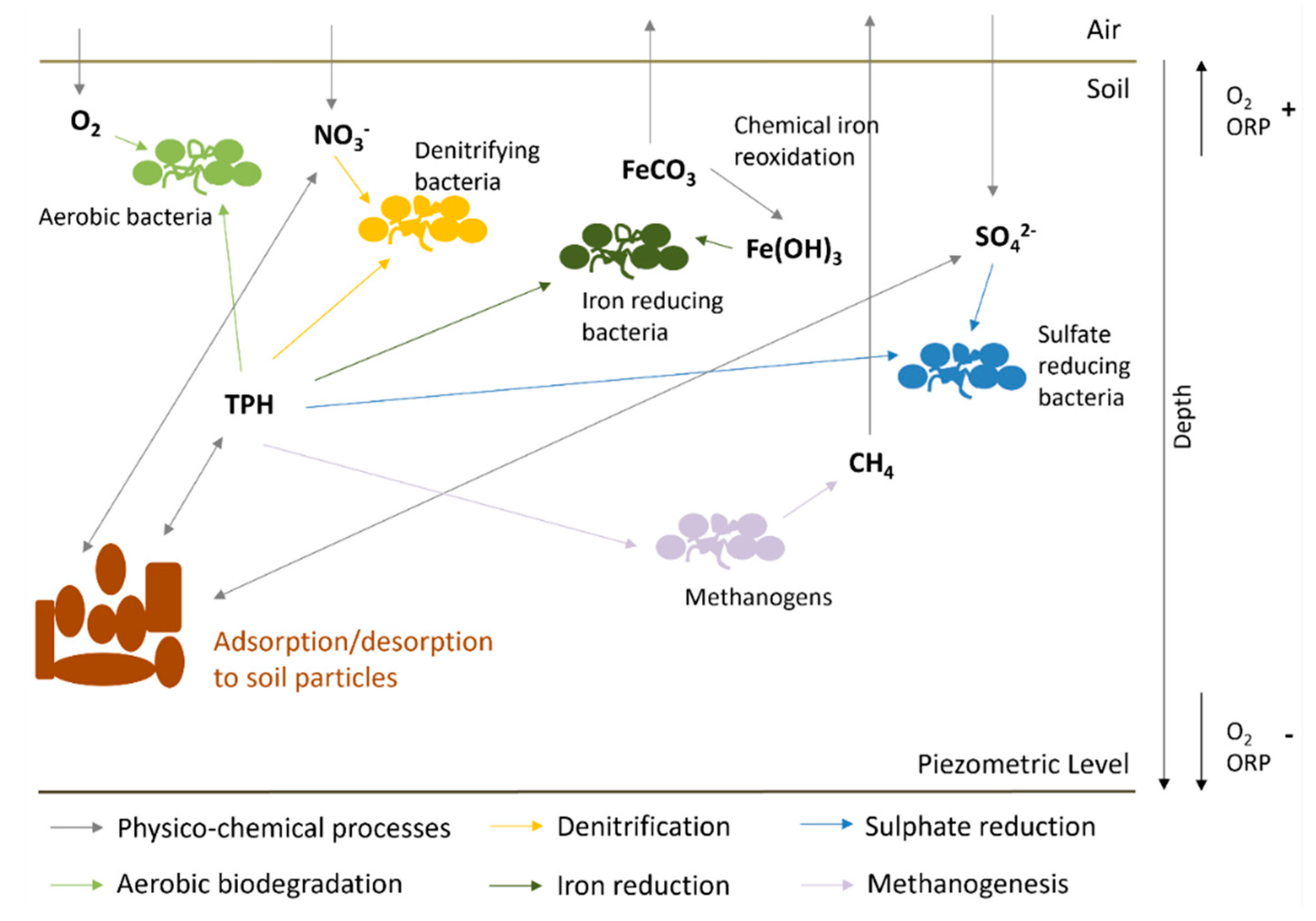
The model is able to calculate phase concentrations and fluxes as a function of space (soil column depth) and time for the different components. In the present model, hydrocarbons biodegradation processes were based on the availability of different electron acceptors (Figure 1).

Briefly, the presented mathematical model considered aerobic and anoxic biodegradation of total petroleum hydrocarbons (TPH), the latter occurring in the presence of iron (III), nitrate or sulfate as electron acceptors. Anaerobic biodegradation of hydrocarbons to methane, which occurs in the absence of any electron acceptor other than bicarbonate/CO₂, was also considered. Hydrocarbon biodegradation to methane is generally performed by complex microbial communities, where close syntrophic relationships between bacteria and methanogenic archaea have been reported as essential [28,29]. Complete hydrocarbon degradation to methane is thermodynamically limited by the activity of the methanogens [29]. Moreover, within anaerobic microbial communities, methanogens are generally the most sensitive and slow-growing microorganisms [30]. Therefore, in this work, petroleum hydrocarbon biodegradation to methane was modelled in only one step, according with the reaction presented in Table S1, admitting that methanogenesis is the limiting step. The model also considered the adsorption/desorption of hydrocarbons, nitrate and sulfate to soil particles as transformation processes. The state variables and the processes rate equations of the developed model are given in

Table 1. State variables.

Variable	Description	Units
$C{H}_4$	Methane concentration in the liquid phase	mg/L
$F{e}^{2+}$	Iron(II) concentration in the liquid phase	mg/L
$C_{N{O}_3^{-}}$	Nitrate concentration in the liquid phase	mg/L
$O_2$	Dissolved oxygen concentration	mg/L
$C_{\mathrm{T}\mathrm{P}\mathrm{H}}$	Total petroleum hydrocarbon concentration in the liquid phase	mg/L
$C_{S{O}_4^{2-}}$	Sulfate concentration in the liquid phase	mg/L
$Fe{\left(OH\right)}_3$	Amorphous iron (III) concentration	g/kg
$S_{N{O}_3^{-}}$	Nitrate concentration in the solid phase	g/kg
$S_{\mathrm{T}\mathrm{P}\mathrm{H}}$	Total petroleum hydrocarbon concentration in the solid phase	g/kg
$S_{S{O}_4^{2-}}$	Sulfate concentration in the solid phase	g/kg
$X_{aer}$	Concentration of aerobic microorganisms	g/kg
$X_{dnb}$	Concentration of denitrifying microorganisms	g/kg
$X_{irb}$	Concentration of iron reducing microorganisms	g/kg
$X_{srb}$	Concentration of sulfate reducing microorganisms	g/kg
$X_{met}$	Concentration of methanogenic microorganisms	g/kg

and

Table 2. Processes rate equations.

Process		Rate Equation
1	Aerobic biodegradation	$r=u_{m\mathrm{a}x,\mathrm{aer}}\left(\frac{C_{\mathrm{TPH}}}{K_{s,\mathrm{TPH}} + C_{\mathrm{TPH}}}\right)\left(\frac{O_2}{K_{s,\mathrm{O}2} + O_2}\right)X_{aer}$
2	Biodegradation coupled to denitrification	$r=u_{m\mathrm{a}x,\mathrm{den}}\left(\frac{C_{\mathrm{TPH}}}{K_{s,\mathrm{TPH}} + C_{\mathrm{TPH}}}\right)\left(\frac{C_{{\mathrm{NO}}_3^{-}}}{K_{s,{\mathrm{NO}}_3^{-}} + C_{{\mathrm{NO}}_3^{-}}}\right)\left(\frac{K_{s,\mathrm{O}2}}{K_{s,\mathrm{O}2} + O_2}\right)X_{\mathrm{dnb}}$
3	Biodegradation coupled to Fe(III) reduction	$r=u_{m\mathrm{a}x,\mathrm{Fe}\left(\mathrm{III}\right)}\left(\frac{C_{\mathrm{TPH}}}{K_{s,\mathrm{TPH}} + C_{\mathrm{TPH}}}\right)\left(\frac{Fe\left(OH\right)}{K_{s, \mathrm{Fe}\left(\mathrm{OH}\right)} + Fe\left(OH\right)}\right)\left(\frac{K_{s,\mathrm{O}2}}{K_{s,\mathrm{O}2} + O_2}\right)X_{\mathrm{irb}}$
4	Biodegradation coupled to sulfate reduction	$r=u_{m\mathrm{a}x,\mathrm{sulf}}\left(\frac{C_{\mathrm{TPH}}}{K_{s,\mathrm{TPH}} + C_{\mathrm{TPH}}}\right)\left(\frac{C_{{\mathrm{SO}}_4^{2-}}}{K_{s,{\mathrm{SO}}_4^{2-}} + C_{{\mathrm{SO}}_4^{2-}}}\right)\left(\frac{K_{s,\mathrm{O}2}}{K_{s,\mathrm{O}2} + O_2}\right)X_{\mathrm{srb}}$
5	Biodegradation under methanogenic conditions	$r=u_{m\mathrm{a}x,\mathrm{met}}\left(\frac{C_{\mathrm{TPH}}}{K_{s,\mathrm{TPH}} + C_{\mathrm{TPH}}}\right)\left(\frac{K_{s,\mathrm{O}2}}{K_{s,\mathrm{O}2} + O_2}\right)X_{\mathrm{met}}$
6	Death of aerobic bacteria	$r=k_{\mathrm{death},\mathrm{X}\_\mathrm{aer}}\times X_{\mathrm{aer}}$
7	Death of denitrifying microorganisms	$r=k_{\mathrm{death},\mathrm{X}\_\mathrm{anae}}\times X_{\mathrm{dnb}}$
8	Death of Fe(III)-reducing microorganisms	$r=k_{\mathrm{death},\mathrm{X}\_\mathrm{anae}}\times X_{\mathrm{irb}}$
9	Death of sulfate-reducing microorganisms	$r=k_{\mathrm{death},\mathrm{X}\_\mathrm{anae}}\times X_{\mathrm{srb}}$
10	Death of methanogenic microorganisms	$r=k_{\mathrm{death},\mathrm{X}\_\mathrm{anae}}\times X_{\mathrm{met}}$
11	Adsorption of hydrocarbon	$r=k\times \left(S_{\mathrm{eq}\_\mathrm{freundlich}\_\mathrm{TPH}}-S_{\mathrm{TPH}}\right)$
12	Adsorption of nitrate	$r=k\times \left(S_{\mathrm{eq}\_\mathrm{freundlich}\_\mathrm{NO}3}-S_{{\mathrm{NO}}_3^{-}}\right)$
13	Adsorption of sulfate	$r=k\times \left(S_{\mathrm{eq}\_\mathrm{freundlich}\_\mathrm{SO}4}-S_{{\mathrm{SO}}_4^{2-}}\right)$
14	Re-oxidation of Fe2+	$r=k_{\mathrm{FeOx}}\times F{e}^{2+}\times O_2$

, respectively. In Annex B of Supporting Information, the full AQUASIM system implementation of the present mathematical model can be consulted. Additionally, the executable file is available in DataRepositoriUM (https://doi.org/10.34622/datarepositorium/2BUM2J, accessed on 28 October 2022).

Simplification assumptions were the following:

(i)

The model considered two phases: one solid, constituted by the soil particles, and another liquid with the water flowing through the soil column. Hydrocarbon might be adsorbed by the soil particles, be dissolved in the water, or float in the NAPL phase (due to its lower density in comparison with water, excess of hexadecane is considered to float, thus forming a free NAPL layer). For simplification, hydrocarbon concentration in the liquid phase refers to the mass of both dissolved and NAPL forms per unit of liquid volume and both are considered to be available for microorganisms growth;

(ii)

Soil temperature was kept constant and equal to 20 °C;

(iii)

Only values for alkanes were considered for all parameters and constants involved in the model processes;

(iv)

For processes of stoichiometric calculations, hexadecane was chosen as a model compound, as alkanes of intermediate chain length are major constituents of petroleum fuels [17]. Thus, processes rates and model parameters were defined following the reactions presented in Table S1;

(v)

Microorganisms do not use any other source of organic matter besides hydrocarbons for growth;

(vi)

The biomass of the hydrocarbon-degrading microorganisms follows growth kinetics according to the Monod equation;

(vii)

To guarantee that all soluble iron does not leave the soil column with the water flow, and due to the fast transformation process of Fe²⁺ and its unstable nature in the environment [31], it was assumed to be a process for iron oxidation in the presence of O₂. This process was considered a first order reaction for Fe²⁺ and O₂ (

Table 3. Initial conditions and input variables.

Name	Description	Value	Unit	Reference
A	Soil column cross sectional area	1	m2
CCH4,in	Input methane concentration	0	mg/L
CFe (II),in	Input iron(II) concentration	0	mg/L
CNO3,in	Input nitrate concentration	0	mg/L
CNO3,ini	Initial soluble nitrate concentration	10	mg/L	[33]
CO2,in	Input concentration of dissolved oxygen	10	mg/L
CO2,ini	Initial concentration of dissolved oxygen	10	mg/L
CTPH,in	Input concentration of hydrocarbon	0	mg/L
CSO4,in	Input sulfate concentration	0	mg/L
CSO4,ini	Initial soluble sulfate concentration	10	mg/L	[33]
Q	Precipitation water flowing through the soil column	*	L/d
STPH,ini	Initial TPH concentration	0.6	g/kg
SFe (III),ini	Initial amorphous iron(III) concentration	66.7	g/kg	[34]
SNO3,ini	Initial nitrate concentration in the solid phase	0.3	g/kg	[35]
SSO4,ini	Initial sulfate concentration in the solid phase	0.1	g/kg
T	Temperature	20	°C
Xaer,ini	Initial concentration of aerobic microorganisms	0.08	g/kg
Xdnb,ini	Initial concentration of denitrifying microorganisms	0.04	g/kg
Xirb,ini	Initial concentration of iron(III) reducing microorganisms	0.04	g/kg
Xsrb,ini	Initial concentration of sulfate reducing microorganisms	0.04	g/kg
Xmet,ini	Initial concentration of methanogenic microorganisms	0.02	g/kg

* Values estimated based on the daily average precipitation for the city of Braga during one hydrological year.

).

Simplifications (ii) and (iii) make the results presented here specific to saturated hydrocarbons but the entire model design applies to any hydrocarbon or mixture of hydrocarbons by simply changing the values of parameters, constants and processes rates. In addition, the present model is considered a wet soil mainly composed of fine sand and/or pumices [32]. However, soil properties can be easily changed by assuming new values for soil porosity and soil density.

For the simulation of a real contamination, the model assumed an oil spill that resulted in a TPH concentration in the soil of 0.6 g/kg for an area of 1 m² and 2 m² soil column depth. In the model development, it was also considered the daily rainfall for the city of Braga (with an annual average of ~3.75 L/d) as an additional flow of water to the soil column (Q in Equation (1)). All input and initial variables are presented in Table 3. Stoichiometric and composition matrix are shown in supplementary material (Table S2).

2.2. Sensitivity Analysis

A sensitivity analysis of the model parameters was carried out using the absolute–relative sensitivity function—Sens AR [25]. The Sens AR measures the absolute change in a state variable for a 100% change in a model parameter and does not depend on the parameter units [27]. The parameters are varied independently to assess how these changes affect the model results. The calculations were performed with AQUASIM for all model parameters present in Table S3.

2.3. Data Collection and Model Calibration

Model parameters and boundary conditions were gathered from the literature and from a set of batch experiments described in Section 2.3.1 and Section 2.3.2. With this approach, the developed model is assumed to be calibrated. Table S3 presents the values of all model parameters.

2.3.1. Solid–Liquid Partition Experiment

Hydrocarbon adsorption to soil particles was assessed in batch assays, using serum bottles of 70 mL total volume. The assays were performed in quadruplicate. Hexadecane (C16:0) (ACROS ORGANICS, 99%) was chosen as a model compound due to its relative abundance in crude oil (up to 50% of the hydrocarbon fraction) [17,36] and its intermediate molecular weight (226.44 g/mol) [17]. Soil was collected from an agricultural site in Barcelos, Portugal, at approximately 1.5 m depth using hand augers. Soil samples were kept at 4 °C, thoroughly homogenized through a 2 mm sieve and characterized. The soil presented a moisture of 2.5 ± 0.05% (w/w), an organic matter content of 0.28 ± 0.004%, pH of 5.2 ± 0.2 (in water) and a silt loam texture from 25% clay, 65% silt and 8.5% sand.

In each bottle, a 1:1 soil-water mixture was prepared [37] with 20 g of dry soil and 20 g of distilled water. Additionally, 100 μL of sodium azide (0.2%, w/v) was used as a microbial activity inhibitor [38]. Different amounts of hexadecane (2.5, 5, 10, 25 and 50 mg) were added with a glass syringe. These corresponded to the following concentrations, expressed relatively to the amount of soil added: 0.125 g/kg, 0.25 g/kg, 0.5 g/kg, 1.25 g/kg and 2.5 g/kg. Blank assays without hexadecane were also prepared. All bottles were closed with Viton rubber stoppers and were kept at 20 °C, 200 rpm, for 7 days. This time period was defined based on preliminary tests carried out to guarantee that adsorption equilibrium was reached. Afterward, the liquid and solid phases were separated by decantation. The liquid phase was acidified at pH 2.0 with HCl and preserved at 4 °C until further hydrocarbon analysis. The hexadecane present in the solid phase was immediately extracted and quantified.

2.3.2. Biodegradation Experiments

Hydrocarbon biodegradation tests were carried out in batch experiments in the presence of oxygen or nitrate as electron acceptors. Sludge (17 ± 2 g/L of volatile solids, VS) from a full-scale treatment plant performing ex situ bioremediation of petroleum-contaminated groundwater, located in France, was used as inoculum. In each bottle, 10 mL of the inoculum was mixed with 35 mL of mineral bicarbonate-buffered culture medium supplemented with salts and vitamins (without reducing agent), prepared as described in [39]. The presence of a solid phase was accomplished by also adding to the bottles 20 g (dry sweight) of sediment from the reservoir of Alto Lindoso dam (Lima River, Portugal). The sediment presented an organic matter content of 5.5 ± 0.5% and a pH of 6.8. Nitrate, sulfate and phosphate concentrations in the sediment’s pore water were lower than the minimum values measurable by the used methods (i.e., 1 mg/L for nitrate, 40 mg/L for sulfate and 0.15 mg/L for phosphate). This sediment was used in the assays, instead of the soil used in the experiments described in Section 2.3.1, with the aim of guaranteeing and reinforcing the microbial hydrocarbon-degrading activity. Hydrocarbon-degrading microorganisms were expected, due to the presence of oil from the motors of boats in this dam.

To have a complex hydrocarbon mixture, the concentrated oily fraction of a produced water (PW) was used as the hydrocarbon source. PW density was 0.75 g/cm³, with a total petroleum hydrocarbon (TPH) concentration of 202 g/L [40]. A PW mass equivalent to 50 mg TPH was added to each bottle, corresponding to a final TPH concentration of approximately 2.5 g/kg (expressed relatively to the dry weight of sediment).

In the anoxic assays, nitrate (20 mmol/L final concentration) was added as an electron acceptor. Bottles (250 mL total volume) were closed with Viton rubber stoppers and aluminum crimp caps, pressurized with N₂/CO₂ (80:20%, v/v) at 1.7 bar (final pressure), and incubated in the dark at 37 °C on a horizontal shaker (110 rpm) for 90 days. In the aerobic assays (oxygen as electron acceptor), the tests were performed by adapting the Biochemical Oxygen Demand (BOD) Oxitop^® method [41]. Briefly, the amount of dissolved oxygen that is consumed during the aerobic biological oxidation is quantified by measuring the negative pressure values generated in the headspace of the bottles. The measuring units (heads) automatically record the pressure values once a day, which are converted into digits and showed in a display. Whenever the Oxitop^® value did not increase by about 5% from the previous value, the bottle was opened, replenishing the available oxygen, and the NaOH pellet (which removes from the headspace the CO₂ released during microbial oxidation) was replaced by a new one. The aerobic assays were incubated in the dark, at 30 °C for 90 days with agitation. All the assays were made in duplicate.

Throughout the incubation time, NO₃⁻ concentration were periodically measured in the anoxic assays. In the aerobic tests, Oxitop^® values were regularly recorded and the cumulative oxygen consumption was calculated by the sum of the Oxitop^® value after multiplication by the corresponding conversion factor.

2.3.3. Analytical Methods

The water and organic matter content in the soil and sediment samples were determined with gravimetry [42] through drying the samples at 105 °C for 24 h and subsequent ignition at 550 °C for 2 h. Volatile solids were determined according to the Standard Methods [43]. Soil texture was evaluated by separating the relative proportions of sand, silt and clay using grading sieves. Nitrate, sulfate and phosphate concentrations were determined using spectrophotometric measurement kits (HACH-LANGE, Germany): LCK 339, range 1–60 mg/L for nitrate; LCK 153, range 40–150 mg/L for sulfate; LCK 349, range 0.15–4.50 mg/L for phosphate. DR2800 spectrophotometer (HACH-LANGE, Düsseldorf, Germany) was used in these analyses. The pH was measured with an inoLab^® pH 7110 bench meter (WTW, Weilheim, Germany).

Hexadecane was quantified in solid and liquid phases. Quantification in solid phase was performed by extracting the hydrocarbon with a mixture of hexane and acetone (1:1) in closed Schott flasks at room temperature for 4 h at 180 rpm [44]. Hexadecane in liquid samples was sequentially extracted three times with hexane, using separatory funnels [45]. All the extracts were cleaned using Sep-Pak Florisil^® cartridges (Waters, Milford, MA, USA) and evaporated in TurboVap^® LV (Biotage, Uppsala, Sweden). Hexadecane concentration was quantified by gas chromatography (GC) in a Varian 4000 GC/MS equipped with a BRUKER BR-1ms column. The injector temperature was set at 250 °C. The temperature of the oven started at 60 °C for 1 min, and then increased up to 170 °C through a temperature ramp of 8 °C/min, holding then at 170 °C for 1 min. Airflow rate was 1 mL/min and the flame ionization detector (FID) temperature was 315 °C [46].

2.4. Model Simulation and Hypothetical Bioremediation Scenarios

Five bioremediation scenarios were developed and compared with the baseline scenario (i.e., the scenario keeping the initial conditions and mimicking the natural attenuation) in order to understand the effect of the different electron acceptors in the biodegradation of saturated hydrocarbons and to demonstrate that the developed model provided a coherent response to external perturbations. The first scenario considered a re-aeration process ($r=K_{La}(O_{2,\mathrm{sat}}-O_2$) with an oxygen mass transfer coefficient ($K_{La}=1$ d⁻¹ [47]) in order to increase the dissolved oxygen concentration in the soil column. This scenario foresees that oxygen will be flushed into the soil column. In the second, third and fourth scenarios, initial concentrations of nitrate, sulfate or iron (III) that were 100 times higher than in the baseline scenario were simulated (i.e., 1000 mg/L for nitrate or sulfate and 6.6 kg/kg for iron). The fifth scenario considered the use of the adsorbed TPH by microorganisms at a rate of approximately 10% of the biodegradation rate that occurs in the liquid phase. This scenario was coded as 10%_STPH and could reflect, for example, the addition of surfactants to contaminated soil.

3. Results

3.1. Solid-Liquid Partition Experiment

In this experiment, the aqueous and non-aqueous liquids were not separated; as such, the amount of hexadecane retrieved from the liquid phase accounts for the dissolved and NAPL forms of this compound. Considering the physical-chemical properties of hexadecane, i.e., low water solubility (9.0 × 10⁻⁴ mg/L at 20 °C), low vapour pressure (1.9 × 10⁻¹ Pa at 20 °C) and predicted log Kow = 8.6 and Koc = 2.9 × 10³ L/kg [48], adsorption to the organic carbon in soil can be mainly expected to occur.

The mass of hexadecane recovered from the solid and liquid (aqueous and non-aqueous) phases, relativel to the different amounts added, are shown in supplementary material (Figure S1). More than 61% of the hexadecane added was retrieved from the solid phase, while only 1 to 4% was quantified in the liquid phase (

Table 4. Hexadecane recovery (%) from the solid and liquid phases and total recovery in the partition experiments.

Mass Added (mg)	Recovery from Solid Phase (%)	Recovery from Liquid Phase (%)	Total Recovery (%)
2.5	77.5 ± 28.0	1.6 ± 0.4	79.1 ± 28.0
5	107.6 ± 0.7	1.3 ± 0.8	108.9 ± 1.0
10	71.7 ± 2.8	4.2 ± 0.4	75.9 ± 2.8
25	61.1 ± 2.0	2.7 ± 0.4	63.9 ± 2.0
50	69.6 ± 5.2	2.4 ± 0.2	71.9 ± 5.2

), showing that this compound mostly adsorbed soil particles for all the concentrations tested. Total hexadecane recovery, calculated by the sum of the mass obtained from both solid and liquid phases, ranged from 64% to 109% (Table 4).

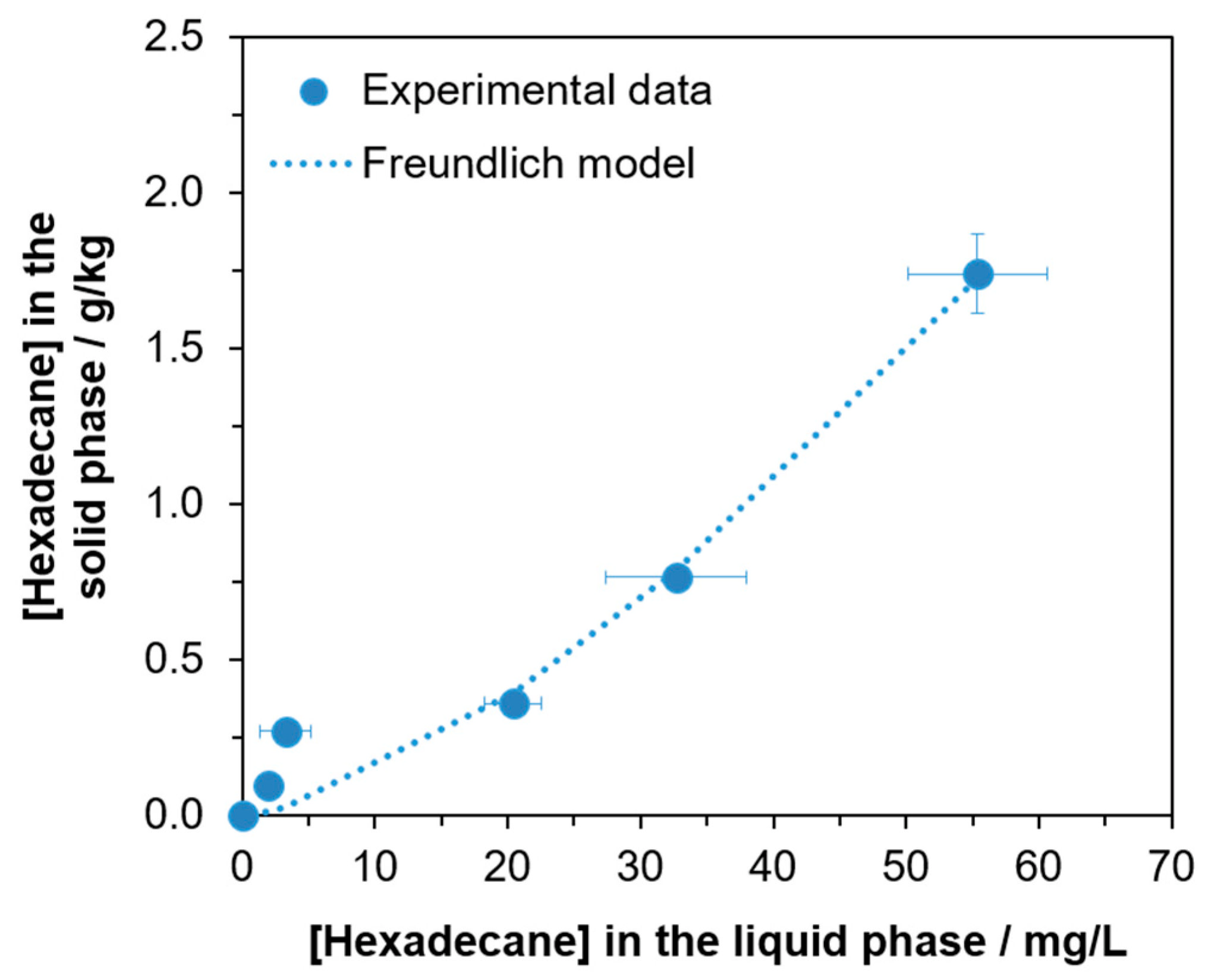
In Figure 2, the distribution of hexadecane concentration between solid and liquid matrices is presented, highlighting once more the tendency of hexadecane for partitioning into the soil. The experimental results were adjusted to a Freundlich isotherm (Equation (2)) [49]. This equation is used here to describe the distribution of hexadecane in the soil (solid phase) versus in the liquid (aqueous and non- aqueous) phase. In this experiment,

$$S=K_f{C}^{\frac{1}{n}}$$

(2)

where S is the hexadecane concentration adsorbed on the solid phase (g/kg), C is the remained hexadecane concentration in the liquid (aqueous and non- aqueous phase) (g/L) and K_f and n are constants, specific for the adsorbate and adsorbent at a given temperature. The obtained parameters were: K_f = 0.004355 L/kg and n = 0.6712, with a R² of 0.97. This correlation coefficient is satisfactory, suggesting that the Freundlich model can adequately describe hexadecane sorption characteristics.

The ratio between the concentration of hexadecane adsorbed in soil and remaining in the liquid phase increases with the increase of hexadecane concentration, resulting in a convex curve (Figure 2). Therefore, for higher initial hexadecane concentrations, this compound will tend to adsorb more in soil and remain less in the liquid phase. This can possibly relate to the fact that at higher hexadecane concentrations, the surface of the soil particles may become covered by this compound, which potentially facilitates additional adsorption. Since in Figure 2 a plateau was not reached, the sorption capacity of the soil was not limited under the range of concentrations studied.

3.2. Biodegradation Assays

In the hydrocarbon biodegradation assays, a rapid increase of the Oxitop values (i.e., a fast oxygen consumption) and a decrease of NO₃⁻ concentrations were verified in the aerobic and anoxic assays, respectively, during the first 30–40 days of incubation (data not shown). This was probably due to the oxidation of more biodegradable substrates from the sediment and inoculum sludge. The same inoculum already showed similar behavior in previous experiments [50]. Therefore, this initial period was not considered for the calculation of the hydrocarbon biodegradation rates.

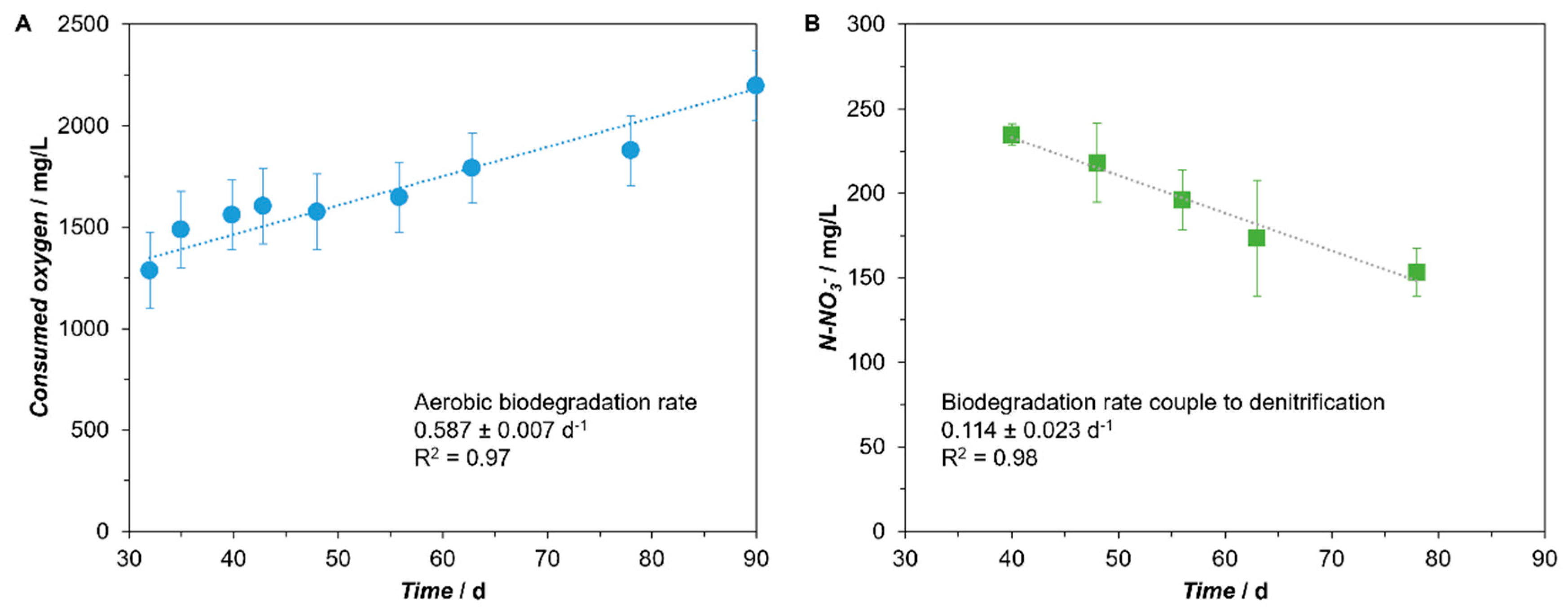
From day 32 and until the end of the test, the oxygen consumed increased gradually in the aerobic assays (Figure 3A), while in the anoxic tests NO₃⁻ concentrations decreased consistently after the first 40 days of incubation (Figure 3B), pointing to the occurrence of aerobic and denitrifying hydrocarbon biodegradation activity. From the curves slope, the corresponding biodegradation rates were obtained and are depicted in the Figure 3. For the calculation of biodegradation rates, the stoichiometry of the chemical reactions presented in Table S1 was considered.

Regarding the biodegradation rate in the presence of oxygen, a wide range of values have been reported by several authors, depending on the substrate and experimental conditions applied. For example, aerobic biodegradation rate of diesel could range from 0.074 d⁻¹ to 0.35 d⁻¹ [14], while other studies present values ranging from 0.587 d⁻¹ to 4.75 d⁻¹ for petroleum hydrocarbons and diesel [7,51]. The value obtained in this work is in line with those from the literature. Regarding the values in the presence of nitrate, Roy and Greer [52] reported a higher rate (0.91 d⁻¹) for hexadecane mineralisation in the presence of NaNO₃, while Bregnard et al. [53] reported values around 0.14 to 0.35 d⁻¹.

3.3. Mathematical Model Development

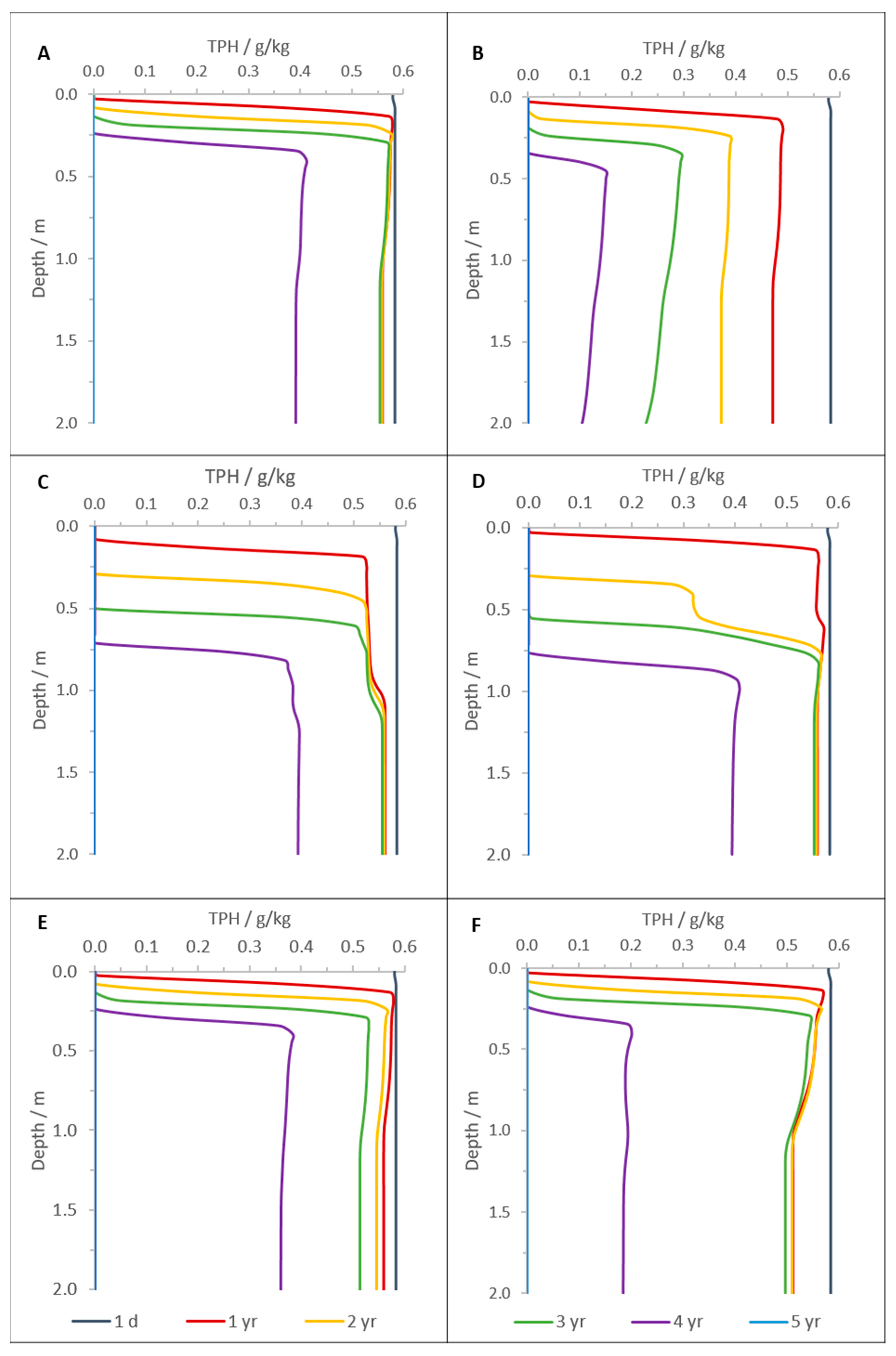
The developed mathematical model was able to predict the variation of hydrocarbon and electron acceptors concentrations, over time and at different depths. As shown in Figure 4, hydrocarbon concentrations decreased over time, both in the solid (STPH) and liquid (CTPH) phases. In the first 0.1 m depth, the decrease of STPH starts slowly and accelerates afterwards (Figure 4A), reaching 50% of the initial value after ~1.2 years (439 days). For depths higher than 0.4 m (Figure 4A,C), STPH remains relatively constant for 3.2 years (1150 days), after which it decreases consistently, reaching a 50% reduction approximately one year later (1507 days). In the liquid phase, the decrease of hydrocarbon concentration follows a similar tendency (Figure 4B,D); here, ~2.3 years (850 days) or ~4.5 years (1626 days) are necessary to reach TPH concentrations lower than 1.0 mg/L, at 0.1 m depth or at depths higher than 0.4 m, respectively. After 5 years, hydrocarbons are almost completely removed from both phases, at any depth (Figure 4).

The top layers of the soil column are the first to show low TPH concentrations (Figure 4C,D), which may result from hydrocarbons biodegradation by aerobic and/or anoxic microorganisms. However, dissolved oxygen concentration rapidly decreases in depth (Figure S2A), e.g., it reaches null values after 1 day for depths higher than 0.1 m, which limits aerobic biodegradation. As the first layers of the soil column became free of hydrocarbons, oxygen concentration increases again along the time. For example, O₂ values close to 10 mg/L are observed in the first 10–20 cm of the soil column after 3–4 years, and up to ~90 cm depth after 5 years (Figure S2A). Aerobic biomass exhibits a peak after 1 year at ~25 cm depth and decreases afterwards (Figure S2B). At higher depth (up to 0.5 m) aerobic biomass also grows, but to a less extent and more slowly than in the upper layers (Figure S2B). Nitrate, sulfate and iron are also rapidly consumed by microbial biomass, soon becoming limiting for TPH biodegradation (Figure S3).

All these results point that, besides biodegradation, the decrease of STPH and CTPH in the first layers of the soil column is most probably due to transport phenomena. To verify this, a new simulation was then performed considering only the adsorption/desorption and transport processes (i.e., all the biodegradation processes were not included). As observed in Figure 5, the profile of STPH and CTPH in the first layers of the soil column (<0.2 m) is very similar to the ones obtained when microbial activity is also considered (Figure 4), highlighting that desorption and transport are the main processes influencing TPH removal over time for the top layers of soil. In addition, Péclet number (Pe) was calculated to verify if diffusion or advection was the most important transport phenomenon in the soil column. Thus, assuming a mass diffusion coefficient for hexadecane of 4 × 10⁻¹⁰ m²/s [54] and an average water inflow of 3.75 L/d, the Pe was 217, meaning that the advective transport predominates over diffusion in the mass transport process.

In deeper soil layers (>0.4 m), however, when just adsorption/desorption and transport processes are considered, STPH and CTPH only begin to decrease after 4 years (Figure 5). By comparison, with Figure 4A,B, it seems that microbial activity has an important role and accelerates TPH removal at higher depths. In fact, after this same time period, STPH was already reduced by 40% at 0.4 m depth when biodegradation was also taken into account (Figure 4A). Since oxygen, nitrate, iron or sulfate are not available below 0.4 m depth at 3–4 years (Figure S3), TPH biodegradation is possibly related with the activity of the methanogens.

Methane concentration presents a long lag phase and starts to increase in the third year of simulation (Figure S4). This is in agreement with the literature, since it has been previously reported that the onset of methanogenic hydrocarbon degradation is often preceded by extended lag phases [55]. The observed lag phase was related with (i) the small initial concentration of methanogenic microorganisms and (ii) substrate utilization by other microbial groups. Only when denitrification, iron reduction and sulfate reduction become limited by the lack of electron acceptors, does methanogenesis start (Figures S3 and S4). This tendency was previously reported in contaminated aquifers [56] and as such it can be expected to happen also in soils. Theoretically, the redox cascade will flow from aerobic degradation, to denitrification, iron(III) reduction, sulfate reduction and finally methanogenesis, determined by the availability of electron acceptors [56]. In this work, the decreased time of hydrocarbon concentration in depth (Figure 4) is closely associated with the methane concentrations in the soil column, which increases exponentially at ~3.5 years and reaches the highest values around 4.4 years for depths higher than 1 m (Figure S4). These results show that methanogenesis has a high impact on TPH concentration and, therefore, TPH biodegradation under methanogenic conditions appears to be the main process contributing for TPH removal at deeper layers of the soil. Methanogenesis was previously shown to be important in the natural attenuation of hydrocarbon contaminated soils [57,58].

3.3.1. Sensitivity Analysis

The results of the sensitivity analysis (summarised for the top 5 parameters with higher sensitivity in

Table 5. Top five values of absolute-relative sensitivity (Sens AR) of model parameters on TPH concentration in the liquid and solid phases (expressed as mg/L and g/kg, respectively).

Rank	CTPH		STPH
	Parameter	Sensitivity (mg/L)	Parameter	Sensitivity (g/kg)
1	$n_{\mathrm{T}\mathrm{P}\mathrm{H}}$	79.07	$u_{\mathrm{m}\mathrm{a}\mathrm{x},\mathrm{met},20}$	1.305
2	$u_{\mathrm{m}\mathrm{a}\mathrm{x},\mathrm{met},20}$	67.64	$n_{\mathrm{T}\mathrm{P}\mathrm{H}}$	1.004
3	$K_{\mathrm{f},\mathrm{T}\mathrm{P}\mathrm{H}}$	15.73	θ	0.239
4	θ	11.49	$k_{\mathrm{death},{\mathrm{X}}_{\mathrm{anae}},20}$	0.215
5	$k_{\mathrm{death},{\mathrm{X}}_{\mathrm{anae}},20}$	11.21	θ	0.211

), carried out to assess the effect of the different parameters on the concentration of TPH in the solid and liquid phases, are presented in Table S4 and corroborate the results described in the previous section. The two parameters from hydrocarbon adsorption isotherm (K_f,TPH and n_TPH) are among the most sensitive parameters, demonstrating the importance of adsorption/desorption for the dynamics of TPH in the soil column, both for C_TPH and for S_TPH. In addition, the maximum TPH biodegradation rate under methanogenic conditions (μ_max,met,20) is the most sensitive parameter for adsorbed TPH (S_TPH, Table 5). As such, STPH is highly dependent of TPH biodegradation coupled to the activity of methanogenic microorganisms. This is possibly related to the fact that, as hydrocarbons are consumed and converted into methane, their concentration in the liquid phase decreases, which facilitates the subsequent desorption and increases their availability to biodegradation. The death rate for anaerobic microorganisms is also a very sensitive parameter, which is most probably linked with the high sensitivity of maximum TPH biodegradation rate under methanogenic conditions. Soil porosity (θ) and soil density (ρ) are also very sensitive parameters, showing the importance of both soil physical properties, and of the physicochemical processes.

3.3.2. Bioremediation Scenarios

Different bioremediation strategies were implemented and the results are depicted in Figure 6. Similar to the previous results, close to the surface (at 0.1 m depth), all scenarios predicted more than 83% TPH removal after two years of simulation (

Table 6. Percentage of TPH removal from solid phase for each scenario during the simulation time.

Depth	Scenario	1 Year	2 Year	3 Year	4 Year	5 Year
0.1 m	Baseline	21.9%	83.7%	100.0%	100.0%	100.0%
	Oxygen	39.8%	97.7%	100.0%	100.0%	100.0%
	Nitrate	82.1%	100.0%	100.0%	100.0%	100.0%
	Sulfate	24.6%	100.0%	100.0%	100.0%	100.0%
	Iron(III)	21.9%	84.3%	100.0%	100.0%	100.0%
	10%_STPH	23.3%	84.8%	100.0%	100.0%	100.0%
0.5 m	Baseline	4.4%	4.5%	5.3%	32.3%	100.0%
	Oxygen	19.0%	35.4%	51.5%	74.9%	100.0%
	Nitrate	12.4%	12.6%	100.0%	100.0%	100.0%
	Sulfate	7.1%	46.2%	100.0%	100.0%	100.0%
	Iron(III)	4.4%	6.7%	12.0%	36.9%	100.0%
	10%_STPH	7.9%	8.0%	10.3%	67.8%	100.0%
1 m	Baseline	6.7%	6.6%	7.2%	33.8%	100.0%
	Oxygen	20.8%	36.8%	54.4%	76.9%	100.0%
	Nitrate	7.8%	9.4%	11.4%	36.2%	100.0%
	Sulfate	6.7%	6.6%	7.2%	32.3%	100.0%
	Iron(III)	6.7%	8.9%	14.0%	38.7%	100.0%
	10%_STPH	14.7%	14.5%	15.9%	67.7%	100.0%
1.5 m	Baseline	6.8%	6.9%	7.7%	34.9%	100.0%
	Oxygen	21.5%	37.8%	57.8%	79.7%	100.0%
	Nitrate	6.8%	6.9%	7.7%	34.3%	100.0%
	Sulfate	6.8%	6.9%	7.7%	34.1%	100.0%
	Iron(III)	6.8%	9.1%	14.5%	39.8%	100.0%
	10%_STPH	14.9%	15.1%	17.3%	69.2%	100.0%
2 m	Baseline	6.8%	6.9%	7.7%	34.9%	100.0%
	Oxygen	21.5%	37.8%	62.0%	82.6%	100.0%
	Nitrate	6.8%	6.9%	7.7%	34.5%	100.0%
	Sulfate	6.8%	6.9%	7.7%	34.4%	100.0%
	Iron(III)	6.8%	9.1%	14.5%	39.9%	100.0%
	10%_STPH	14.9%	15.1%	17.3%	69.3%	100.0%

The color gradient means the following: red—low removal rate; green—high removal rate.

). In fact, in the scenario with a high concentration of nitrate, after one year a TPH removal of around 82% can be observed. In these first soil layers (<0.5 m), the high TPH removal can be attributed to the presence of the electron acceptors but also to adsorption/desorption and transport processes as previously discussed. In depth, clear differences between the different scenarios can be observed. The implementation of a soil aeration mechanism (Figure 6B) resulted in a faster TPH removal. After one year of the oil spill, the TPH removal was already higher than 19% at 0.5 m depth, reaching values above 50% after 3 years in the presence of oxygen, nitrate and sulfate (Table 6). In the scenarios with the addition of a high concentration of nitrate or sulfate, the results show that near the surface (0.1 m) the model predicts the complete TPH removal in two years (Figure 6C,D, Table 6). These results are in agreement with the literature results, since increasing concentrations of electron acceptors promotes an increase in biodegradation rates [10,33]. For deeper layers, the removal was lower, mainly due to the depletion of the electron acceptor. Indeed, neither nitrate nor sulfate reaches the end of soil column, meaning that this will not be a problem in terms of groundwater contamination.

For the scenario with higher initial iron (III) concentration in the soil column (Figure 6E), the results showed similar behavior to the baseline scenario. At surface layers, it is expected to be a 100% removal; for deeper layers (>0.25 m), the TPH removal was not very high (maximum of 40% after four years), although an increase in removal over time was generally observed (Table 6).

Some authors suggested that adsorbed hydrocarbons are also directly available for microorganisms [21,22,59]. Thus, a scenario where the microorganisms can use the TPH adsorbed to soil (scenario 10%_S_TPH), though at a lower rate, was designed (Figure 6F). The results showed higher removal efficiencies than in the base scenario but lower that in the high NO₃ and high SO₄ scenarios, in the first layers (Table 6). For depths higher than 1 m, two times higher TPH removal is predicted, relative to the high NO₃ and high SO₄ scenarios (Table 6). This scenario could reflect, for example, the addition of surfactants to contaminated soil. Surfactants reduce the interfacial` tension, increasing the solubility and bioavailability of hydrocarbons, thus facilitating their transport and biodegradation [5,51].

In summary, and based on mathematical model results, soil re-aeration and surfactants (oxygen and 10%_S_TPH scenarios) addition are the bioremediation strategies that will guarantee a faster treatment of the oil spill. Nevertheless, the natural attenuation (baseline scenario) could also be considered to be applied, since the technical and economic issues involved in soil re-aeration and the application of dissolved compounds could be challenging.

Very few examples of mathematical models were completely validated for one or two bioremediation methodologies [14]. In the present study, and to overcome the difficulty of model validation, we determined the adsorption isotherm for hexadecane as a major compound of petroleum hydrocarbons (sensitivity analysis showed that adsorption is a very important process) and calculated the biodegradation rate of a complex hydrocarbon mixture in the presence of oxygen or nitrate.

Experimental databases from which to verify and/or calibrate the model are lacking, but sensitivity analyses and the different prospective scenarios developed helped to parameterize and validate the model. In addition, sensitivity analysis provided important information towards the identification of important parameters to be determined in future experiments. The fact that model assumptions are flexible, as well as the modular nature of the mathematical model implemented in AQUASIM, make it possible to be applied to other situations such as mixed reactors and sediment column modeling.

The benefit from such endeavor was the development of a modeling tool capable to predict the fate of hydrocarbons in situ, in a contaminated soil column. With the present mathematical modeling, a series of bioremediation scenarios (alternatives involving a spectrum of electron acceptors application schemes) could be designed prior to in situ implementation. In this manner, bioremediation options for petroleum-contaminated soils might be made comparable in an engineering (and economic) sense [15].

4. Conclusions

The results from the batch experiments showed that hexadecane mostly adsorb on soil particles (>60%) for all the concentrations tested. Oxygen and nitrate are effective electron acceptors for hydrocarbon removal, with experimentally estimated biodegradation rates of 0.587 ± 0.007 d⁻¹ and 0.114 ± 0.023 d⁻¹, respectively.

The mathematical modelling predicted well the expected biodegradation processes in soil. The activity of the different microbial groups is determined by the availability of the electron acceptors, following the classical redox cascade (aerobic degradation, to denitrification, iron (III) reduction, sulfate reduction and finally methanogenesis). In the baseline scenario, hydrocarbon degradation under methanogenic conditions, as well as adsorption/desorption and washout by the water flux, exert a higher influence on hydrocarbon removal.

Physicochemical parameters such as porosity, soil density and adsorption isothermal parameters presented high sensitivity, thus requiring careful definition and, if needed, further investigation for real case implementation of the model.

For practical purposes, this model can be used as a support tool for the management of contaminated sites, since it allows the simulation and comparison of different bioremediation strategies, namely the addition of different electron acceptors, including soil re-aeration (that can stimulate a specific microbial group, relative to the others) or surfactants addition (that may also accelerate soil bioremediation by increasing hydrocarbons bioavailability), among others. Different bioremediation scenarios were simulated and pointed to natural attenuation or soil re-aeration being the best strategies under the simulated conditions. The addition of surfactants will also accelerate soil bioremediation.

Finally, this study demonstrates that a mathematical model capable of responding to environmental perturbation can work as a decision-supporting tool for the proper design of soil bioremediation strategies tackling petroleum hydrocarbon contamination.

References

- Pérez, A.P.; Rodríguez Eugenio, N. Status of Local Soil Contamination in Europe—Revision of the Indicator “Progress in the Management Contaminated Sites in Europe”; EUR 29124 EN; Publications Office of the European Union: Luxembourg, 2018; ISBN 9789279800726. [Google Scholar]
- Van Liedekerke, M.; Prokop, G.; Rabl-Berger, S.; Kibblewhite, M.; Louwagie, G. Progress in Management of Contaminated Sites; European Commission, Joint Research Centre, Institute for Environment and Sustainability: Ispra, Italy, 2014. Available online: https://www.sepa.gov.rs/download/lbna26376enn.pdf (accessed on 15 September 2022).
- Koshlaf, E.; Ball, A.S. Soil bioremediation approaches for petroleum hydrocarbon polluted environments. AIMS Microbiol. 2017, 3, 25–49. [Google Scholar] [CrossRef]
- Hentati, O.; Lachhab, R.; Ayadi, M.; Ksibi, M. Toxicity assessment for petroleum-contaminated soil using terrestrial invertebrates and plant bioassays. Environ. Monit. Assess. 2013, 185, 2989–2998. [Google Scholar] [CrossRef]
- Ali, N.; Bilal, M.; Khan, A.; Ali, F.; Iqbal, H.M.N. Effective exploitation of anionic, nonionic, and nanoparticle-stabilized surfactant foams for petroleum hydrocarbon contaminated soil remediation. Sci. Total Environ. 2020, 704, 135391. [Google Scholar] [CrossRef]
- Varjani, S.J. Microbial degradation of petroleum hydrocarbons. Bioresour. Technol. 2017, 223, 277–286. [Google Scholar] [CrossRef]
- Gogoi, B.K.; Dutta, N.N.; Goswami, P.; Krishna Mohan, T.R.; Gogoi, B.; Dutta, N.; Goswami, P.; Mohan, T. A case study of bioremediation of petroleum-hydrocarbon contaminated soil at a crude oil spill site. Adv. Environ. Res. 2003, 7, 767–782. [Google Scholar] [CrossRef]
- Ebadi, A.; Khoshkholgh Sima, N.A.; Olamaee, M.; Hashemi, M.; Ghorbani Nasrabadi, R. Remediation of saline soils contaminated with crude oil using the halophyte Salicornia persica in conjunction with hydrocarbon-degrading bacteria. J. Environ. Manag. 2018, 219, 260–268. [Google Scholar] [CrossRef]
- Zhang, B.; Zhang, L.; Zhang, X. Bioremediation of petroleum hydrocarbon-contaminated soil by petroleum-degrading bacteria immobilized on biochar. RSC Adv. 2019, 9, 35304–35311. [Google Scholar] [CrossRef] [Green Version]
- Margesin, R.; Zimmerbauer, A.; Schinner, F. Monitoring of bioremediation by soil biological activities. Chemosphere 2000, 40, 339–346. [Google Scholar] [CrossRef]
- Carberry, J.B.; Wik, J. Comparison of ex situ and in situ bioremediation of unsaturated soils contaminated by petroleum. J. Environ. Sci. Health-Part A Toxic/Hazard. Subst. Environ. Eng. 2001, 36, 1491–1503. [Google Scholar] [CrossRef]
- Ojewumi, M.E.; Emetere, M.E.; Babatunde, D.E.; Okeniyi, J.O. In Situ Bioremediation of Crude Petroleum Oil Polluted Soil Using Mathematical Experimentation. Int. J. Chem. Eng. 2017, 2017, 5184760. [Google Scholar] [CrossRef]
- Alridha, A.H.; Al-jilawi, A.S.; Alsharify, F.H.A. Review of Mathematical Modelling Techniques with Applications in Biosciences. Iraqi J. Comput. Sci. Math. 2022, 3, 135–144. [Google Scholar] [CrossRef]
- Fernández, E.L.; Merlo, E.M.; Mayor, L.R.; Camacho, J.V. Kinetic modelling of a diesel-polluted clayey soil bioremediation process. Sci. Total Environ. 2016, 557–558, 276–284. [Google Scholar] [CrossRef]
- Nicol, J.-P.; Wise, W.R.; Molz, F.J.; Benefield, L.D. Modeling biodegradation of residual petroleum in a saturated porous column. Water Resour. Res. 1994, 30, 3313–3325. [Google Scholar] [CrossRef]
- Geng, X.; Boufadel, M.C.; Personna, Y.R.; Lee, K.; Tsao, D.; Demicco, E.D. BIOB: A mathematical model for the biodegradation of low solubility hydrocarbons. Mar. Pollut. Bull. 2014, 83, 138–147. [Google Scholar] [CrossRef]
- Potter, D.L.; Simmons, K.E. Analysis of Petroleum Hydrocarbons in Environmental Media; Weisman, W., Ed.; Amherst Scientific Publishers: Amherst, MA, USA, 1998; Volume 1, ISBN 1884940145. [Google Scholar]
- Ebenhöh, W.; Berthe-Corti, L. Modelling of hexadecane degradation in continuous-flow cultures. BioSystems 2001, 59, 159–183. [Google Scholar] [CrossRef]
- Kosterin, A.V.; Sofinskaya, O.A. Simulation of tridecane degradation under different soil water contents. Eurasian Soil Sci. 2010, 43, 712–718. [Google Scholar] [CrossRef]
- Uzukwu, C.; Dionisi, D. Comparison of the Biodegradation of n-alkanes and Readily Biodegradable Substrates Using Open Mixed Culture under Aerobic, Anoxic and Anaerobic Conditions. Int. J. Environ. Bioremediat. Biodegrad. 2017, 5, 65–76. [Google Scholar] [CrossRef] [Green Version]
- Park, J.H.; Zhao, X.; Voice, T.C. Biodegradation of non-desorbable naphthalene in soils. Environ. Sci. Technol. 2001, 35, 2734–2740. [Google Scholar] [CrossRef]
- Woo, S.H.; Park, J.M.; Rittmann, B.E. Evaluation of the interaction between biodegradation and sorption of phenanthrene in soil-slurry systems. Biotechnol. Bioeng. 2001, 73, 12–24. [Google Scholar] [CrossRef]
- Shyh-Yau, W.; Cumaraswamy, V. Biodegradation of Naphthalene-Contaminated Soils in Slurry Bioreactors. J. Environ. Eng. 2001, 127, 748–754. [Google Scholar] [CrossRef]
- Reichert, P. AQUASIM—A tool for simulation and data analysis of aquatic systems. Water Sci. Technol. 1994, 30, 21–30. [Google Scholar] [CrossRef]
- Martins, G.; Ribeiro, D.C.C.; Pacheco, D.; Cruz, J.V.V.; Cunha, R.; Gonçalves, V.; Nogueira, R.; Brito, A.G.G. Prospective scenarios for water quality and ecological status in Lake Sete Cidades (Portugal): The integration of mathematical modelling in decision processes. Appl. Geochem. 2008, 23, 2171–2181. [Google Scholar] [CrossRef] [Green Version]
- Vera, L.; Martel, G.; Gutierrez, J.; Márquez, M.; Abreu Acosta, N.; Salas, J.J.; Sardón, N.; Herrera Melián, J.A.; Aguilar Bujalance, M.E.; Rexachs, J.A.; et al. Sustainable Management of Wastewater in Rural Zones: DEPURANAT Project (Gestión Sostenible del Agua Residual en Entornes Rurales: Proyecto DEPURANAT); Institute of the Canaries (Instituto Tecnológico de Canárias): Las Palmas de Gran Canaria, Spain, 2006; pp. 111–153. ISBN 84-690-2232-6. [Google Scholar]
- Reichert, P. Aquasim 2.0-User Manual, Computer Program for the Identification and Simulation of Aquatic Systems; EAWAG: Dübendorf, Switzerland, 1998; ISBN 3-906484-16-5. [Google Scholar]
- Gieg, L.M.; Fowler, S.J.; Berdugo-Clavijo, C. Syntrophic biodegradation of hydrocarbon contaminants. Curr. Opin. Biotechnol. 2014, 27, 21–29. [Google Scholar] [CrossRef]
- Jiménez, N.; Richnow, H.H.; Vogt, C.; Treude, T.; Krüger, M. Methanogenic Hydrocarbon Degradation: Evidence from Field and Laboratory Studies. Microb. Physiol. 2016, 26, 227–242. [Google Scholar] [CrossRef]
- Chen, Y.; Cheng, J.J.; Creamer, K.S. Inhibition of anaerobic digestion process: A review. Bioresour. Technol. 2008, 99, 4044–4064. [Google Scholar] [CrossRef]
- Heron, G.; Crouzet, C.; Bourg, A.C.M.; Christensen, T.H. Speciation of Fe(II) and Fe(III) in Contaminated Aquifer Sediments Using Chemical Extraction Techniques. Environ. Sci. Technol. 1994, 28, 1698–1705. [Google Scholar] [CrossRef]
- Gödeke, S.; Vogt, C.; Schirmer, M. Estimation of kinetic Monod parameters for anaerobic degradation of benzene in groundwater. Environ. Geol. 2008, 55, 423–431. [Google Scholar] [CrossRef]
- Dou, J.; Li, S.; Cheng, L.; Ding, A.; Liu, X.; Yun, Y. The Enhancement of Naphthalene Degradation in Soil by Hydroxypropyl-β-Cyclodextrin. Procedia Environ. Sci. 2011, 10, 26–31. [Google Scholar] [CrossRef] [Green Version]
- Mielki, G.F.; Novais, R.F.; Ker, J.C.J.C.; Vergütz, L.; de Castro, G.F.; Vergütz, L.; de Castro, G.F. Iron Availability in Tropical Soils and Iron Uptake by Plants. Rev. Bras. Ciênc. Solo 2016, 40. [Google Scholar] [CrossRef] [Green Version]
- Sempere, A.; Oliver, J.; Ramos, C. Simple determination of nitrate in soils by second-derivative spectroscopy. J. Soil Sci. 1993, 44, 633–639. [Google Scholar] [CrossRef]
- Head, I.M.; Jones, D.M.; Röling, W.F.M. Marine microorganisms make a meal of oil. Nat. Rev. Microbiol. 2006, 4, 173–182. [Google Scholar] [CrossRef]
- Limousin, G.; Gaudet, J.-P.; Charlet, L.; Szenknect, S.; Barthès, V.; Krimissa, M. Sorption isotherms: A review on physical bases, modeling and measurement. Appl. Geochem. 2007, 22, 249–275. [Google Scholar] [CrossRef]
- Lichstein, H.C. Studies of the Effect of Sodium Azide on Microbic Growth and Respiration: III. The Effect of Sodium Azide on the Gas Metabolism of B. subtilis and P. aeruginosa and the Influence of Pyocyanine on the Gas Exchange of a Pyocyanine-Free Strain of P. aerugino. J. Bacteriol. 1944, 47, 239–251. [Google Scholar] [CrossRef] [Green Version]
- Stams, A.J.M.; Van Dijk, J.B.; Dijkema, C.; Plugge, C.M. Growth of syntrophic propionate-oxidizing bacteria with fumarate in the absence of methanogenic bacteria. Appl. Environ. Microbiol. 1993, 59, 1114–1119. [Google Scholar] [CrossRef] [Green Version]
- Silva, R.M.; Fernandes, A.M.; Fiume, F.; Castro, A.R.; Machado, R.; Pereira, M.A. Sequencing batch airlift reactors (SBAR): A suitable technology for treatment and valorization of mineral oil wastewaters towards lipids production. J. Hazard. Mater. 2021, 409, 124492. [Google Scholar] [CrossRef]
- Platen, P.H.; Wirtz, A. Applications of Analysis Measurement of the Respiration Activity of Soils Using the OxiTop Control Measuring System Basic Principles and Process Characteristic Quantities; WTW: Weilheim, Germany, 1999; Available online: https://download.sechang.com/pds/2000/2000_18033a.pdf (accessed on 15 September 2022).
- Martins, G.; Henriques, I.; Ribeiro, D.C.; Correia, A.; Bodelier, P.L.E.; Cruz, J.V.; Brito, A.G.; Nogueira, R. Bacterial Diversity and Geochemical Profiles in Sediments from Eutrophic Azorean Lakes. Geomicrobiol. J. 2012, 29, 704–715. [Google Scholar] [CrossRef] [Green Version]
- APHA; AWWA; WPCF. Standard Methods for the Examination of Water and Wastewater; American Public Health Association: Washington, DC, USA, 1999; ISBN 0875532357. [Google Scholar]
- Siddique, T.; Rutherford, P.M.; Arocena, J.M.; Thring, R.W. A proposed method for rapid and economical extraction of petroleum hydrocarbons from contaminated soils. Can. J. Soil Sci. 2006, 86, 725–728. [Google Scholar] [CrossRef]
- EPA. Method 3510C: Separatory Funnel Liquid-Liquid Extraction; United States Environmental Protection Agency: Washington, DC, USA, 1996; pp. 1–8. [Google Scholar]
- Paulo, A.M.S.; Salvador, A.F.; Alves, J.I.; Castro, R.; Langenhoff, A.A.M.; Stams, A.J.M.; Cavaleiro, A.J. Enhancement of methane production from 1-hexadecene by additional electron donors. Microb. Biotechnol. 2018, 11, 657–666. [Google Scholar] [CrossRef] [Green Version]
- Shin, W.S.; Park, J.C.; Pardue, J.H. Oxygen dynamics in petroleum hydrocarbon contaminated salt marsh soils: III. A rate model. Environ. Technol. 2003, 24, 831–843. [Google Scholar] [CrossRef]
- EPA. CompTox Chemicals Dashboard. Available online: https://comptox.epa.gov/dashboard/ (accessed on 17 March 2022).
- Sparks, D.L. 5—Sorption Phenomena on Soils. In Environmental Soil Chemistry, 2nd ed.; Academic Press: Burlington, VT, USA, 2003; pp. 133–186. ISBN 978-0-12-656446-4. [Google Scholar]
- Martins, V.R.; Martins, G.; Castro, R.; Pereira, L.; Alves, M.M.; Cavaleiro, A.J.; Soares, O.S.G.P.; Pereira, M.F.R. Microbial conversion of oily wastes to methane: Effect of ferric nanomaterials. In Wastes: Solutions, Treatments and Opportunities III, Proceedings of the 5th International Conference Wastes 2019, Lisbon, Portugal, 4–6 September 2019; Vilarinho, C., Castro, F., Gonçalves, M., Fernando, A.L., Eds.; Taylor & Francis Group: Leiden, The Netherlands, 2020; pp. 339–345. ISBN 978-0367-25777-4. [Google Scholar]
- Whang, L.M.; Liu, P.W.G.; Ma, C.C.; Cheng, S.S. Application of biosurfactants, rhamnolipid, and surfactin, for enhanced biodegradation of diesel-contaminated water and soil. J. Hazard. Mater. 2008, 151, 155–163. [Google Scholar] [CrossRef]
- Roy, R.; Greer, C.W. Hexadecane mineralization and denitrification in two diesel fuel-contaminated soils. FEMS Microbiol. Ecol. 2000, 32, 17–23. [Google Scholar] [CrossRef]
- Bregnard, T.P.A.; Höhener, P.; Zeyer, J. Bioavailability and biodegradation of weathered diesel fuel in aquifer material under denitrifying conditions. Environ. Toxicol. Chem. 1998, 17, 1222–1229. [Google Scholar] [CrossRef]
- Geerdink, M.J.; Van Loosdrecht, M.C.M.; Luyben, K.C.A.M. Model for microbial degradation of nonpolar organic contaminants in a soil slurry reactor. Environ. Sci. Technol. 1996, 30, 779–786. [Google Scholar] [CrossRef]
- Siddique, T.; Penner, T.; Semple, K.; Foght, J.M. Anaerobic Biodegradation of Longer-Chain n-Alkanes Coupled to Methane Production in Oil Sands Tailings. Environ. Sci. Technol. 2011, 45, 5892–5899. [Google Scholar] [CrossRef]
- Lovley, D.R. Anaerobes to the Rescue. Science 2001, 293, 1444–1446. [Google Scholar] [CrossRef] [Green Version]
- Anderson, R.T.; Lovley, D.R. Hexadecane decay by methanogenesis. Nature 2000, 404, 722–723. [Google Scholar] [CrossRef]
- Sherry, A.; Grant, R.J.; Aitken, C.M.; Jones, M.; Bowler, B.F.J.; Larter, S.R.; Head, I.M.; Gray, N.D. Methanogenic crude oil-degrading microbial consortia are not universally abundant in anoxic environments. Int. Biodeterior. Biodegrad. 2020, 155, 105085. [Google Scholar] [CrossRef]
- Mukherji, S.; Weber, W.J., Jr. Mass transfer effects on microbial uptake of naphthalene from complex NAPLs. Biotechnol. Bioeng. 2001, 75, 130–141. [Google Scholar] [CrossRef] [Green Version]
- Hamdi, W.; Gamaoun, F.; Pelster, D.E.; Seffen, M. Nitrate sorption in an agricultural soil profile. Appl. Environ. Soil Sci. 2013, 2013, 597824. [Google Scholar] [CrossRef] [Green Version]
- Alves, M.E.; Lavorenti, A. Sulfate adsorption and its relationships with properties of representative soils of the São Paulo State, Brazil. Geoderma 2004, 118, 89–99. [Google Scholar] [CrossRef]
- Suarez, M.P.; Rifai, H.S. Biodegradation rates for fuel Hydrocarbons and Chlorinated Solvents in groundwater. Bioremediat. J. 1999, 3, 337–362. [Google Scholar] [CrossRef]
- Ma, T.T.; Liu, L.Y.; Rui, J.P.; Yuan, Q.; Feng, D.S.; Zhou, Z.; Dai, L.R.; Zeng, W.Q.; Zhang, H.; Cheng, L. Coexistence and competition of sulfate-reducing and methanogenic populations in an anaerobic hexadecane-degrading culture. Biotechnol. Biofuels 2017, 10, 207. [Google Scholar] [CrossRef]
Figure 1.
Schematic representation of hydrocarbon biodegradation processes considered in the mathematical model.
Figure 2.
Hexadecane partition between solid and liquid (aqueous and non-aqueous) phases. The results presented are the average and standard deviation for quadruplicate assays.
Figure 3.
Cumulative oxygen consumption over time in the aerobic assays (A), and time course of NO3− concentrations (expressed as N) in the anoxic assays (B).
Figure 4.
Variation of hydrocarbon concentration over time (top) and in depth (bottom), in the solid phase (A,C) and in the liquid phase (B,D).
Figure 5.
Variation of hydrocarbon concentration over time, in the solid (A) and in the liquid phase (B), considering only the adsorption/desorption and transport processes.
Figure 6.
Concentration of TPH in solid and liquid phase; (A) baseline scenario; (B) re-aeration scenario; (C) high NO3− scenario; and (D) high SO42− scenario; (E) high Fe (III) scenario; (F) 10% STPH scenario.