An Attention-Based Deep Convolution Network for Mining Airport Delay Propagation Causality

Abstract

The airport network is a highly dynamic and complex network connected by air routes, and it is difficult to study the impact of delays at one airport on another airport by means of human intervention. Due to the delay propagation law contained in the delay time series, some studies have used Granger causality and transfer entropy to explore whether there is a causal relationship between any two airports. However, no research has yet established a delay causal network from the perspective of the airport network as a whole. To this end, an attention mechanism is introduced into the deep convolutional network architecture, and a deep temporal convolution prediction model considering the attention mechanism is proposed, so as to establish the relationship between different airport delay time series under the same network architecture. According to the attention factor score, the delay propagation causality between airports is preliminarily screened, and the direct causality is verified based on a t-test and propagation delay analysis. Taking China’s civil airport network as an example, the method proposed in this paper can not only discover the causal relationship of delays between airports but also characterize the strength of the relationship. Further analysis found that each airport is affected by an average of six airports, and airports with small delays are more likely to be affected by other airports.

1. Introduction

With the rapid development of the civil aviation transportation industry, the contradiction between flight slot demand and airspace resources has become increasingly prominent. This has resulted in congested airspace, especially at some large airports, and flight delays have become the norm [1]. Flight delays have many negative impacts on passengers, airlines, and the civil aviation industry. For passengers, flight delays disrupt their itinerary and bring great inconvenience to them. For airlines, on the one hand, flight delays affect the travel experience of passengers, and passengers may choose other airlines or modes of transportation, resulting in a drop in passenger flow and huge economic losses to airlines. On the other hand, each aircraft is scheduled to fly multiple segments every day, and the arrival delay of the previous segment has a certain impact on the departure and arrival of the subsequent segment. In the long run, flight delays will affect the development of the civil aviation industry. For example, in China, with the rapid development of high-speed railways, some short-distance passengers gradually flow to railway transportation, which makes civil aviation transportation gradually lose its advantages. In the past two decades, a large number of researchers have studied the problem of flight delays, and have also proposed many effective methods and measures to solve the problem of delay [2,3]. However, due to the rapid development of the civil aviation industry and the rapid increase in the number of flights, many of the methods previously proposed are no longer applicable [4]. For example, flight slot optimization methods at the strategic level and flight scheduling methods at the tactical level can reduce flight delays to a certain extent, but these methods may not work when the number of flights increases to a certain extent [5,6]. Therefore, in the development process of the civil aviation industry, flight delay has always been a difficult problem that needs to be challenged.

The reasons for initial flight delays are attributed to five categories: air carrier delays, extreme weather delays, the national aviation system, aircraft late arrival, and safety [7]. Since airports are connected by air routes and have connectivity in resources, initial flight delays may cause flight delays at the destination airport, and delays may spread to other associated airports, spreading throughout the airport network from the time that the initial delay is caused. According to different research objects, the research on delay propagation is divided into the perspective of aircraft and the perspective of airports [8]. From the perspective of aircraft, the main study is how delays are propagated between different segments when a single aircraft is flying multiple segments. These studies provide decision support for airline fleet arrangements [9]. From the airport’s point of view, the main study object is how delays are propagated in the airport network [1,10,11,12,13]. For example, flight delays at an airport will affect related airports and which airports are key nodes in the airport network. Research on these issues will help air traffic management to reduce congestion from the perspective of the entire airport network, while improving operational efficiency and reducing flight delays. This paper focuses on the study of flight delay propagation mechanisms from the perspective of airports. The main goal is to find the causal relationship between airports and the magnitude of the impact, so as to control the level of delay from the perspective of the overall airport network.

At present, researchers mainly analyze airport delay propagation from the aspects of simulating the delay propagation process, airport delay propagation mechanism, and delay propagation causality [13,14,15]. The delay propagation process mainly refers to the study of delay propagation from the perspective of a dynamic process [3,14,16,17,18]. In terms of simulating the delay propagation process, Ciruelos et al. [19] established an agent-based data-driven model to simulate the delay propagation process. Liu et al. [20] constructed a mathematical delay propagation model and a Bayesian network-based arrival delay model according to the relationship between flights to study the relationship between arrival delays. They consider arrival delays as a source of other delays. Among related flights, the spread of arrival delays can exacerbate departure delays at busy hub airports. Delays can be reduced by the availability of scheduled flight schedules, thereby reducing delay propagation. Severe weather can cause huge delays. Fleurquin et al. [21] used a data-driven model to reproduce the delay propagation dynamics in the US airport network. The model focuses on the day of a major storm in the United States. Therefore, it is concluded that bad weather may cause network system congestion, which can be addressed by considering different interventions. After that, Fleurquin et al. defined a metric capable of quantifying the level of network congestion, and found that even under normal operating conditions, there is a nonnegligible risk of system instability. At the same time, they also argue that the connectivity between passengers and crew is the most relevant internal factor for delay propagation [22]. Baspinar et al. [8] analyzed delay propagation from different perspectives, and established two different types of new delay propagation models using the epidemic propagation process. These two types of models are flight-based propagation models and airport-based propagation models. On this basis, they validated the model using European historical track data. Campanelli et al. [23] used two different agent-based models (a first-come-first-served model and an ATFM-based time-planning-first-served model) to simulate delay propagation and assess the impact of network disruptions in the US and European airport networks, and found that a first-come-first-served model resulted in greater delay propagation. Wu et al. [24] used a Bayesian network to build an airline network delay propagation model. The model considers multiple connectivity sources for airlines, including aircraft, crew connections, and passenger connections, which can identify weak links in the flight network based on past flight data. Dai et al. [25] built a heterogeneous network model according to the different connections of departing flights. Departing flights are divided into different clusters according to the connections between them, and the evolution of these clusters in multistage scheduling shows a propagation mechanism. Wu et al. [26] proposed an airport sector network delay model suitable for flight delay estimation in the air transportation network. The model was applied to the 21 busiest airports in China, and by comparing the real delay data with the data estimated by the network delay model, it can be found that the model could well simulate the situation that the airport or airspace may become a delay in the air transportation system [26]. Unlike traditional studies on flight delays, Chen et al. [1]. study the trend of flight delay transmission in a region and show the relationship between delays occurring at multiple airports.

The delay propagation mechanism mainly includes the generation form and propagation mode of delay [3,16,17]. In terms of the delay propagation mechanism, Ahmad Beygi et al. [27] and Ahmad Beygi et al. [13] reallocated existing idle resources to those flights most prone to delay transmission, reducing the impact of the next phase of delays on the airport without changing the personnel and cost of the original plan. Pyrgiotis et al. [10] construct an analytical queuing and network decomposition model to study the complex phenomenon of delay propagation in large airport networks. The stochastic dynamic queuing model treats each airport in the network as a single-server queuing system whose arrival rate obeys negative exponential distribution and service rate obeys Erlang distribution to calculate delays. Approximate network delay models are computationally fast, able to quickly calculate delays due to localized congestion at individual airports and capture the “ripple effects” of delay propagation. Applying the model to a network of 34 of the busiest airports in the United States shows that delay propagation tends to “smooth out” daily airport demand and push more demand into late night hours. Kim et al. [28] displayed the generated delays and the propagated delays on a two-dimensional graph and grouped airports/routes according to the delay characteristics. Ivanov et al. [29] considered controlling the distribution of ATFM delays to minimize the likelihood of delays propagating to subsequent flights. Therefore, they propose a two-layer mixed-integer optimization model to solve the unbalanced problem of route demand and capacity. Minimizing delay propagation by solving the demand and capacity imbalance problem of routes is the first level, and increasing the connectivity of flight slots without increasing delays is the second level.

In recent years, the research community has begun to analyze the delay propagation mechanism from the aspect of airport delay propagation causality mining [15]. Airport delay propagation causality can describe the degree of the direct impact of delays at one airport on another airport. Building an airport delay propagation causal network will help managers understand key nodes in the airport network so that targeted measures can be taken in advance to alleviate air traffic congestion. In addition, the current delay prediction model based on correlation cannot guarantee the robustness of the model. Constructing delay prediction models based on causality is more interpretable and can predict which factors are responsible for the results and when the prediction model will stop working, resulting in more robust predictions.

As the airport network is a highly complex dynamic network, it is difficult to study the impact of one airport’s delay on other airports by means of human intervention. Fortunately, the delay time series implies the law of delay propagation causality, which has been preliminarily explored by some researchers. Some researchers use Granger causality [30] to construct the airport delay propagation network. Zamin et al. [15] regarded the Chinese airport network as a complex network, and used the method of Granger causality tests to study the delay time series between two airport pairs. If the delay time series of airport A is more helpful to predict the delay time series of airport B than the delay time series of airport B itself, it is considered that the delay of airport A is the cause of the delay of airport B. Similarly, Du et al. [31] also established a delay causal network based on Granger causality, and studied the airport delay propagation mechanism by analyzing the topological properties of the network. The causal mining of airport delay propagation based on the Granger causality method can only capture the linear dependence of two airport delay time series. Zhang et al. [32] used transfer entropy to analyze the causal relationship between two airport delay time series, and then quantitatively expressed the degree of influence of one airport’s delay on another airport’s delay. Causal relationship mining based on transfer entropy belongs to a class of nonparametric models that can discover linear and nonlinear dependencies, but cannot handle nonstationary time series.

The airport network is a network composed of a large number of airports passing through the airline network. Due to the dynamic changes of flight information and environmental information, and the nonlinear interaction between airports, the airport network can be regarded as a dynamic and nonlinear complex network system. Given the powerful nonlinear representation ability of deep learning methods, they have been widely used in transportation [33,34,35], energy [36,37], economics [38,39], medical [40,41], and other fields. Recently, in the research on nontemporal causality discovery, the research community has proposed some deep learning models, such as causal effect estimation based on variational autoencoders [42], functional causal model learning based on causal generative neural networks [43], and reconstruction of causal graphs based on structure-independent models [44]. Causal relationship mining methods can be divided into experimental-based methods and observation-based methods.

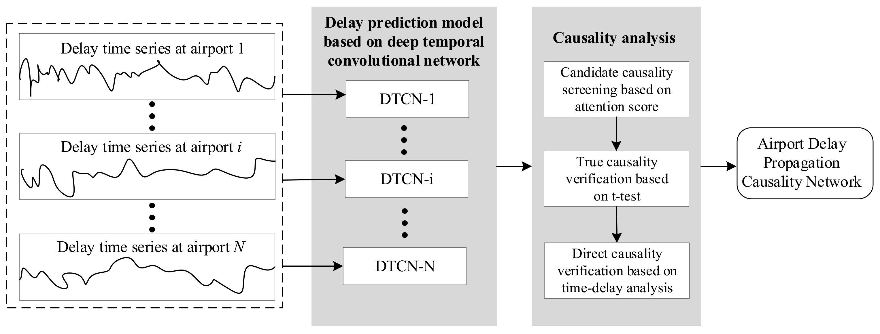
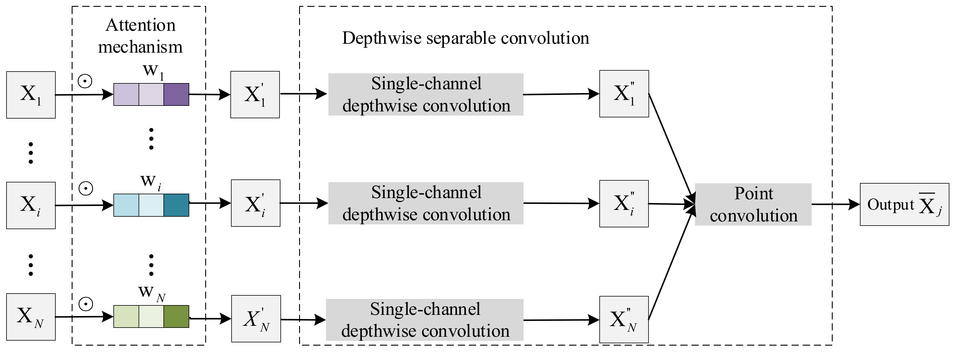
As the airport network is dynamic and complex, it is not feasible to intervene in the actual operation of the airport. Since the delay time series contains the causal law of delay propagation, this paper will study the construction of an airport delay causality network from the perspective of data-driven and airport networks. It is well known that deep convolutional neural networks can characterize the delay time series of a single airport very well. Therefore, under the framework of a deep convolutional network, this paper integrates the delay time series of different airports by introducing an attention mechanism, and establishes a deep convolutional network based on the attention mechanism. The attention mechanism score parameter, like the convolutional network parameter, is learned from the data and can quantitatively characterize the impact of one airport’s delay on another airport. Further, according to the characteristics of the strength of the airport, the score of the attention mechanism can be used to preliminarily screen the airport pairs with delay propagation causality. Finally, direct causality is verified based on a t-test and propagation delay analysis. The causality of delay propagation in China’s airport network is analyzed, and the experimental results obtained are consistent with some mainstream experiences.

The rest of this paper is organized as follows: Section 2 elaborates on the problem of delay propagation causality; the proposed method will be introduced in Section 3, including a delay prediction model based on deep convolutional networks and causality verification based on the attention mechanism and t-test. Section 4 discusses the propagation mechanism of airport network delays by case. Finally, Section 5 summarizes the content of this paper.

2. Problem Formulation

The causal mining of airport delay propagation is to find the delay influence relationship between airports and to depict the extent to which delays at one airport lead to delays at another airport. Specifically, if delays at one airport come first, delays at the other airport come after. At the same time, the first delayed airport has an impact on the later delayed airport and the later delayed airport changes with the first delayed airport. It is considered that there is a delay causal relationship between the two airports, and the delay at the former airport is the cause of the delay at the latter airport. Recently, researchers have given a definition of causality between pairs of airports, that is, if the current and previous delay information of one airport helps explain the delay of another airport at a certain time in the future, then there is a causal relationship between them [15,31,32]. 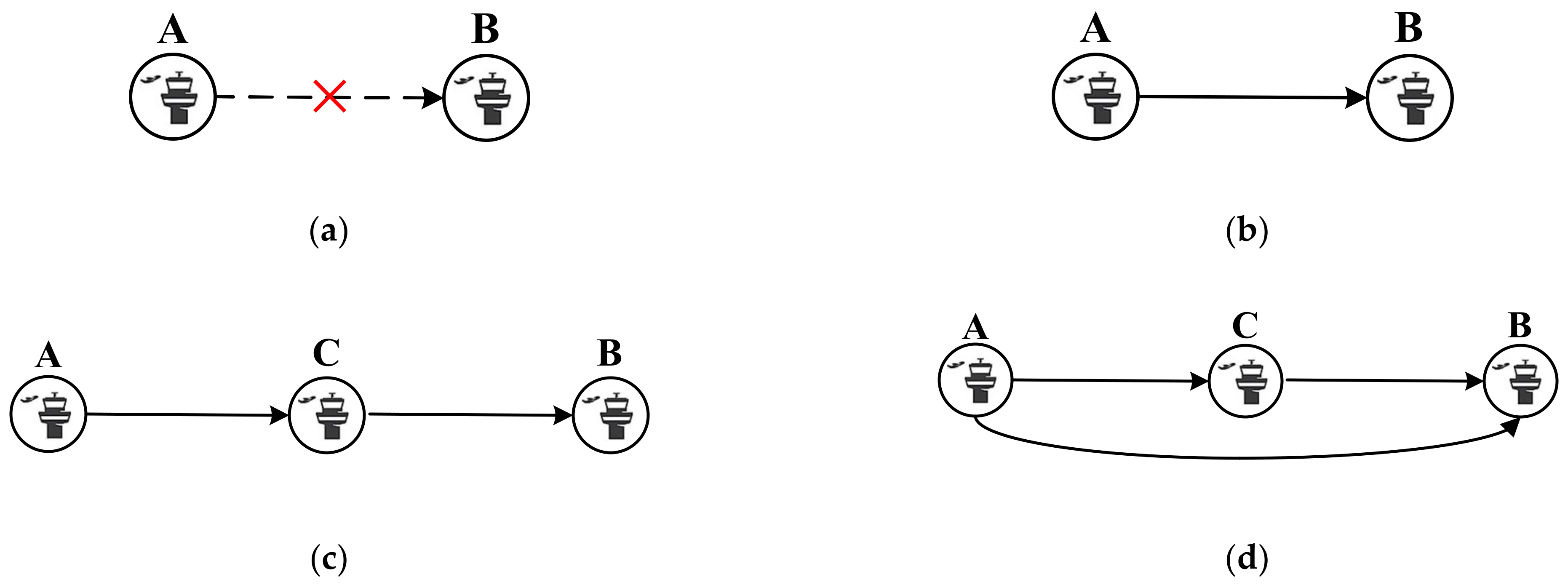As shown in Figure 1, delay causality between airports can be summarized into four forms: no causation, direct causation, indirect causation, and both direct and indirect causation.

Figure 1 shows four forms of airport delay propagation causality. In Figure 1a, a delay at airport A will not affect airport B. In Figure 1b, there is a direct causal relationship between airport A and airport B without intermediary airports, and the delay propagation path is $\mathrm{A}\to \mathrm{B}$. In Figure 1c, there is an indirect causal relationship between airport A and airport B as an intermediate airport C, and the delay propagation path is $\mathrm{A}\to \mathrm{C}\to \mathrm{B}$. It is important to note that there may be multiple indirect causal paths between two airports. In Figure 1d, there are both direct causal paths $\mathrm{A}\to \mathrm{B}$ and indirect causal paths $\mathrm{A}\to \mathrm{C}\to \mathrm{B}$ between airport A and airport B.

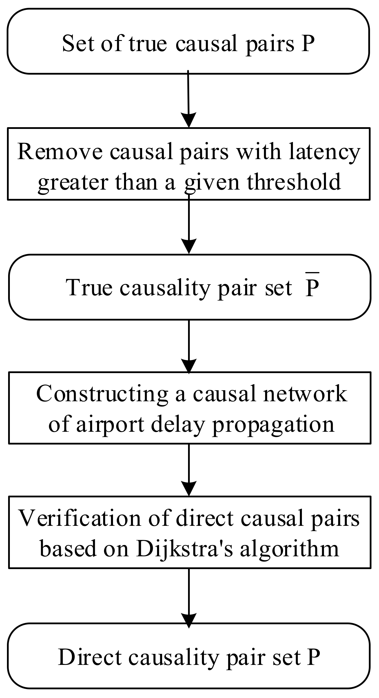
Since the airport network is a network connected by air routes, there may be multiple indirect causal paths between any two airports. Direct causation involves a relationship between two airports, while indirect causation involves three or more airports. From the perspective of air traffic managers, direct causality to guide traffic control is more intuitive and easier to implement than indirect causality. Therefore, this section mainly focuses on the direct causality in the propagation of airport delays, that is, the direct impact of delays at one airport on delays at other airports, which does not consider the indirect effects of delay propagation on subsequent airports.

In order to better represent the causal relationship of an airport network, a weighted directed graph is used to represent the causal relationship network of airport delay propagation. Suppose there are N airports in the airport network. Denote $G=(\mathrm{V},\mathrm{E},\mathrm{D})$ as the airport delay propagation causality network; $\mathrm{V}={\left\{v_i\right\}}_{i=1:N}$ represents the airport set, where $v_i$ represents the feature vector of the airport I; $\mathrm{E}={\left\{e_{ij}\right\}}_{i,j=1:N}$ represents the set of edges in the airport network. If there is a direct causal relationship between the airport $i\to j$, that is, the airport $i$ has an edge pointing to $j$, then $e_{ij}=1$; otherwise, $e_{ij}=0$. $\mathrm{D}={\left\{d_{ij}\right\}}_{i,j=1:N}$ represents the weight set of edges, where $d_{ij}$ represents the weight of edge $e_{ij}$, which means the degree of influence of the airport $i$ on the airport $j$. 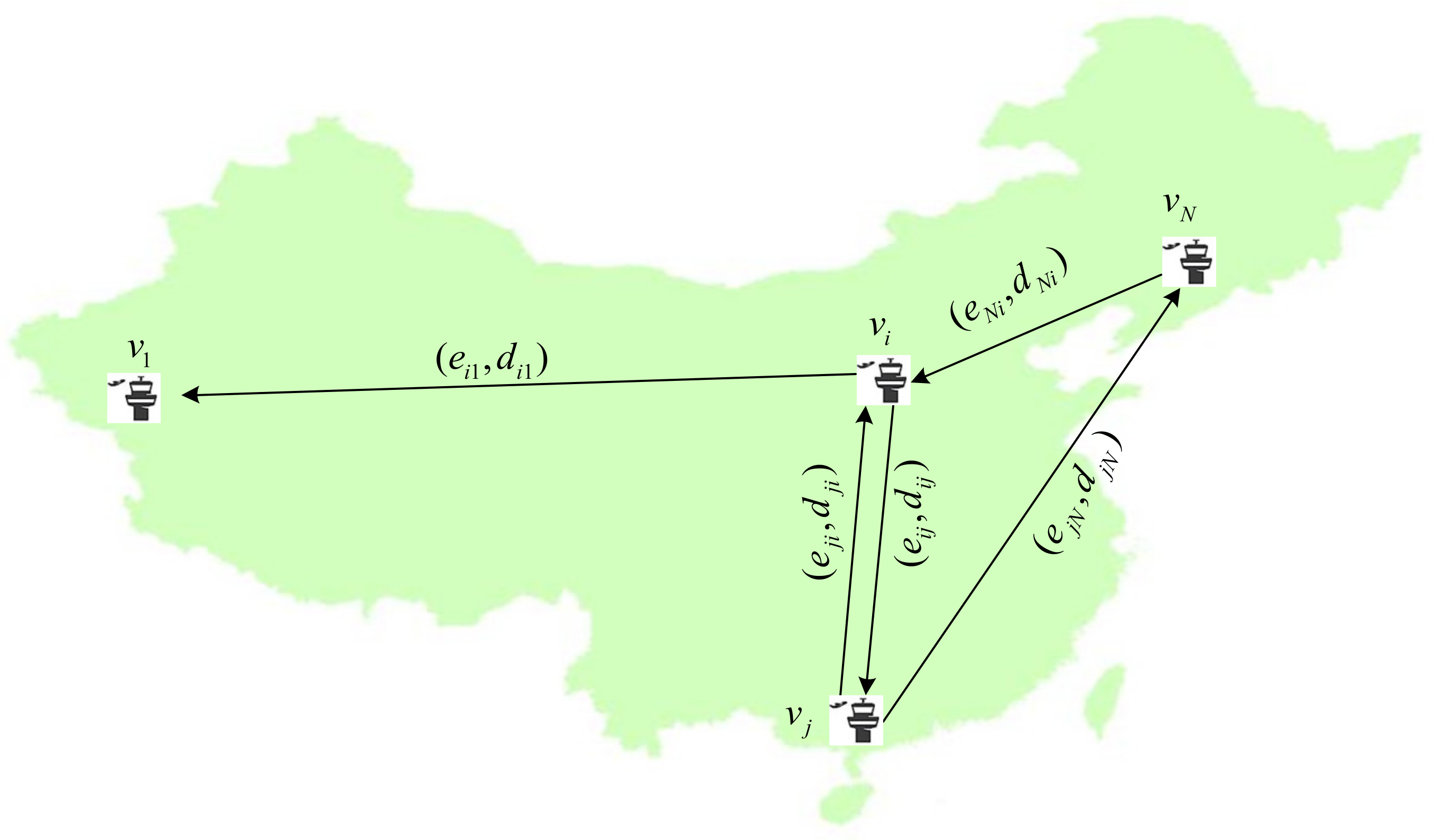Figure 2 is a schematic diagram of the direct causality network of airport delay propagation, in which the arrows point to the direction of delay propagation, and the delay and the degree of influence are given above the arrow. For any two airports, the delay propagation between them can be divided into three cases: there is no delay propagation, the delay propagation is one-way, and the delay propagation is two-way. As shown in Figure 2, the delay propagation between airport $i$ and airport 1 is one-way, between airport $i$ and airport $j$ it is two-way, and there is no delay propagation between airport 1 and airport $j$.

To construct the direct causality network of airport delay propagation as shown in Figure 2, the biggest challenge is how to distinguish direct causality from correlation, indirect causation, and confounding causality:

(a)

How to distinguish causality from correlation. The correlation is a mutual relationship between the delays of two airports, which means that the delay of one airport changes and the other airport also changes. It can be a positive correlation or a negative correlation. The “cause” airport and the “effect” airport in the causal relationship pair of airport delay propagation often show correlation, which can be regarded as a special kind of correlation. Cause and effect are directional, and changes to the cause affect the outcome. Therefore, in order to distinguish the causal relationship from the correlation relationship, it is necessary to observe the delay changes of the “effect” airport after a certain period of time by controlling the delay changes of the “cause” airport.

(b)

How to distinguish direct causation from indirect causation. As shown in Figure 2, the delay at the airport will not directly cause the delay at airport 1, but the delay may be propagated to airport 1 through airport $i$, so there is an indirect causal relationship between airport $N$ and airport 1. Recently, some researchers used Granger causality [15,31] and transfer entropy [32] to judge whether there is a causal relationship between airport pairs and build an airport delay causality network according to the causal relationship between airport pairs. Since the airport network is not treated as a whole when judging causality, it is difficult to find indirect causality. Therefore, in order to better distinguish direct and indirect causality, it is necessary to take all airports into consideration when constructing a causal relationship mining model.

(c)

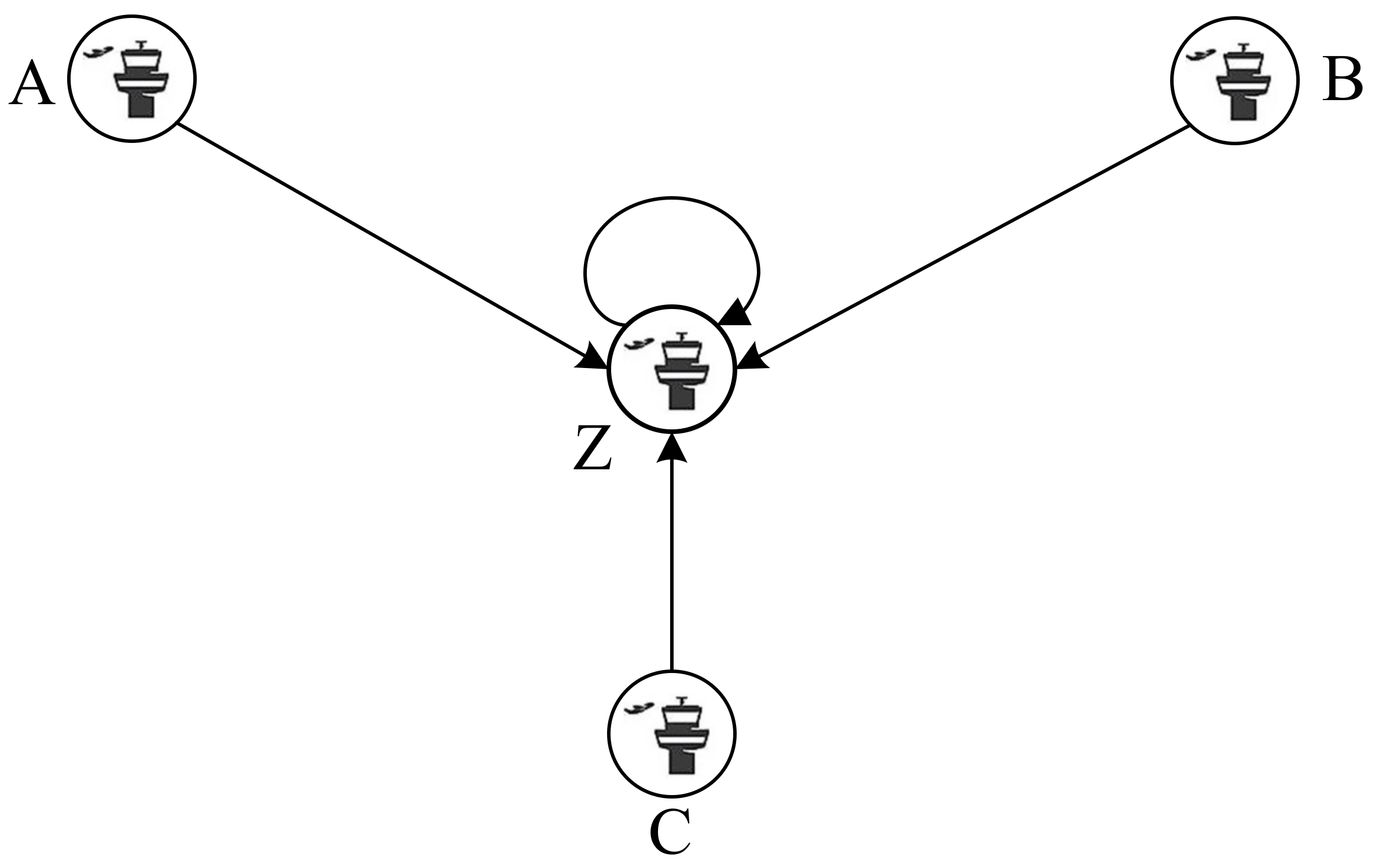
How to measure the influence degree and propagation delay time of multiple “cause” airports on the same “effect” airport. Delays at an airport are often the result of the combined action of multiple airports, including delays at the airport itself. Therefore, this causality is also called confounding causation. Figure 3 is a schematic diagram of multiple airports acting on the same airport. If the delays of airport A, airport B, and airport C are propagated to airport Z simultaneously, then airport A, airport B, and airport C are the “cause” airports of airport Z. It should be noted that due to the specific differences between the three “cause” airports and the “effect” airport Z, there will be differences in the delay time of delay propagation. For example, if the distance from airport A to airport Z is farther than the distance from airport B to airport Z, then delays from airport A will take longer to propagate to airport Z than delays from airport B will take to propagate to airport Z. In Figure 3, there is a closed loop at airport Z, which means delays in past time periods at airport Z itself affect subsequent time periods.

3. Methodology

3.1. Method Overview

The general definition of causality contains the following two characteristics [45]: (a) temporal precedence: the cause occurs before and the effect occurs after, and the chronological order of cause and effect cannot be reversed; (b) physical influence: changing the cause will affect the result, that is, the change in the result caused by the state change in the cause is objective. In view of the characteristic of time sequence, it is easier to take it into account when constructing the causal relationship mining of airport delay propagation based on time series. For example, when constructing the input and output of the model, the delay status information of the “cause” airport and “effect” airport is used as input and output, respectively, but the delay status information of the “effect” airport is later than that of “cause” airport. The difficulty with causality discovery is how to take physical effects into account when building a model.

For the causal discovery of airport delay propagation, the mainstream mining algorithms are divided into two stages: prediction and causality analysis [15,31]. In the first stage, a model that uses the delay time series of the “cause” airport to predict the delay of the “effect” airport is built. However, historical and current delays at one airport help predict future delays at another airport, and there may be a correlation. Therefore, in the second stage, it is necessary to use some criteria to judge the true causal relationship between the airport pairs based on the prediction model. Like the mainstream causality mining algorithm, this paper adopts a two-stage mining idea, as shown in Figure 4. The difference from the existing mainstream methods is that because the airport is a dynamic and complex network, this section builds a model directly from the perspective of the airport network, and establishes a deep temporal convolution network (DTCN) airport delay prediction model. The model takes the delay time series of all airports as model input, which can better capture the interaction between airports. In order to measure the degree of influence of all airports on the target airport, an attention mechanism is introduced into the model, and the degree of influence is quantitatively measured by attention parameters.

In general, the attention parameter measures the strength of the delay correlation between two airports. A large value of the attention parameter indicates a strong correlation; conversely, a small value of the attention parameter indicates a weak correlation. Therefore, when causality is performed in the second stage, the airport pairs with weak correlation are first eliminated according to the value of the attention parameter. On this basis, a candidate causality screening based on attention score is proposed, and the airport pairs with strong correlation are reserved as the candidate causality set. Since the temporal order between airport pairs has been considered in the first stage, in order to judge whether the causal relationship pairs in the candidate causal relationship set are true causal relationships, a true causality verification based on a t-test is proposed. By intervening on delays at “cause” airports, the time series of “cause” airports are randomly permuted and fed into the learned prediction model. The t-test method is used to judge the significance level of the “effect” airport prediction error before and after the sequence rearrangement, and further according to the significance level to judge whether it belongs to the real causal relationship, and finally the airport delay propagation causal relationship set is obtained. Finally, we propose a direct causality verification method based on time-lapse analysis to distinguish direct causality from indirect causality.

3.2. Delay Prediction Model Based on Deep Convolutional Network

This section first expounds on the problem of delay propagation in airport networks and then describes the model architecture for causality mining based on deep convolutional neural networks. Further, this section describes how to train a deep convolutional neural network model and obtain the causal relationship between airports based on the trained model.

3.2.1. Delay Time Series

According to the official definition of a flight delay, the time when the actual execution time of the flight is 15 min after the planned execution time is the flight delay time. This paper studies the delay propagation law between airports. As with other methods of studying this problem, the difference between the actual flight execution time and the planned execution time is used as the flight delay time. Assuming that the airport network contains N airports, with $\Delta t$ as the time step, a day can be divided into T time intervals. For the time step setting, some researchers take 15 min [10,32], and some researchers set it to 60 min [15,31]. Here, 15 min is taken as the time step and divide the day into 96 time intervals. According to the definition of a single flight delay, the average departure delay time series ${\mathbf{X}}_i=[x_i^1,x_i^2,\cdots ,x_i^T]$ of the airport $i$ is constructed, in which $x_i^t$ represents the average delay of all flights in the time period t at the airport $i$. According to the first-come-first-served operation rule, the canceled flight usually does not occupy the resources of the current airport and may not impact the operation of subsequent flights at the current airport, but may have an impact on the destination airport [46]. Therefore, when calculating the average departure delay, canceled flights are considered and they are equivalent to a delay of 180 min [31].

3.2.2. Attention-Based Time Series Prediction Architecture

The goal of airport delay propagation causality discovery is to find directly correlated airports that help predict delays at the target airport. Whether it is the Granger causality test used in the literature [15,31] to find the causality of delayed propagation, or the transfer entropy used in the literature [32], the prediction is essentially the evaluation. These methods are used to examine the variation of delay time series at one airport and whether it is helpful to predict future delays at another airport. However, these methods only mine causal relationships between pairs of airports, without considering the whole airport network, and the mining results may have indirect or confounding causal relationships. This section will comprehensively consider the airport network perspective, and introduce an attention mechanism into the deep time series convolutional network (DTCN). The delay time series of all airports are used as the input of DTCN, and the delay time series of a single airport is used as the output to the airport network. A DTCN prediction model is constructed for each airport, as shown in Figure 5. The processing flow from left to right is to input the delay time series $\{{\mathrm{X}}_1,{\mathrm{X}}_2\cdots ,{\mathrm{X}}_N\}$ of all airports, perform attention mechanism processing on them (obtain the sequence $\{{\mathrm{X}}_1^{\prime },{\mathrm{X}}_2^{\prime },\cdots ,{\mathrm{X}}_N^{\prime }\}$), and perform single-channel depth convolution on each time series (obtain the sequence $\{{\mathrm{X}}_1^{″},{\mathrm{X}}_2^{″},\cdots ,{\mathrm{X}}_N^{″}\}$), and point convolution (output delay prediction vector ${\overline{\mathrm{X}}}_j$ of target airport $j$).

In order to predict the delay in the t-th time interval of the airport, a prediction network is trained for each airport with the delay information of all airports in the ${\tau }_{\max }$ periods before the t-period as input. Let $X_j^{(t-1)}=\left[x_j^{t-{\tau }_{\max }},x_j^{t-{\tau }_{\max }+1},\cdots ,x_j^{t-1}\right]$ represent the delay time subsequence of the airport $j$ in the time interval $\left[t-{\tau }_{\max },t-1\right]$, and the delay prediction model based on the deep time domain convolutional network is expressed as follows:

$$\left[\begin{array}{l}{x}_1^t\\ x_2^t\\ ⋮\\ x_N^t\end{array}\right]=DTCN\left(X_1^{(t-1)},X_2^{(t-1)},\cdots ,X_N^{(t-1)}\right),$$

(1)

where $DTCN\left(\cdot \right)$ represents a deep convolutional network model that needs to be learned.

Equation (1) is a general model and cannot distinguish the influence of input variables on output variables. In order to find the directly related airports that help to predict the delay of the target airport, the input variables need to be separated for model training. N airports need to train N deep time domain convolution prediction models $\left\{DTC{N}_1\left(\cdot \right),DTC{N}_2\left(\cdot \right),\cdots ,DTC{N}_N\left(\cdot \right)\right\}$, then Equation (1) can be written as:

$$\left\{\begin{array}{l}{x}_1^t=DTC{N}_1(X_1^{(t-1)},X_2^{(t-1)},\cdots ,X_N^{(t-1)})\\ \hspace{1em}\hspace{1em}\hspace{1em}\hspace{1em}\hspace{1em}\hspace{1em} ⋮\\ x_j^t=DTC{N}_j(X_1^{(t-1)},X_2^{(t-1)},\cdots ,X_N^{(t-1)})\\ \hspace{1em}\hspace{1em}\hspace{1em}\hspace{1em}\hspace{1em}\hspace{1em} ⋮\\ x_N^t=DTC{N}_N(X_1^{(t-1)},X_2^{(t-1)},\cdots ,X_N^{(t-1)}).\end{array}\right.$$

(2)

Further, an attention mechanism is introduced to measure the impact of delays at different airports on the target airport. For any target airport $j$, an N-dimensional vector ${\mathbf{w}}_j=[w_{1j},w_{2j},\cdots ,w_{Nj}]$ is introduced to perform point-by-point multiplication with the input time series of $N$ airports. Call ${\mathbf{w}}_j$ the attention score vector (or contribution vector) of all airports (including the target airport itself) to the target airport. When the neural network based on the attention mechanism processes a large amount of input information, it will select a part of the key information for processing, and ignore the information that is irrelevant to the output. By visualizing input and output attention, the intuitiveness and interpretability of the network can be improved. This will become an active area in the research community, partly compensating for the lack of interpretability of deep learning.

By introducing the attention mechanism, Equation (2) is rewritten as:

$$\left\{\begin{array}{l}{x}_1^t=DTC{N}_1(w_{11}\odot X_1^{(t-1)},w_{21}\odot X_2^{(t-1)},\cdots ,w_{N1}\odot X_N^{(t-1)})\\ \hspace{1em}\hspace{1em}\hspace{1em}\hspace{1em}\hspace{1em}\hspace{1em} ⋮\\ x_j^t=DTC{N}_j(w_{1j}\odot X_1^{(t-1)},w_{2j}\odot X_2^{(t-1)},\cdots ,w_{Nj}\odot X_N^{(t-1)})\\ \hspace{1em}\hspace{1em}\hspace{1em}\hspace{1em}\hspace{1em}\hspace{1em} ⋮\\ x_N^t=DTC{N}_N(w_{1N}\odot X_1^{(t-1)},w_{2N}\odot X_2^{(t-1)},\cdots ,w_{NN}\odot X_N^{(t-1)}).\end{array}\right.$$

(3)

Note that the prediction target’s own time series and other airport time series are used as input at the same time, so that under the same network architecture, self-causal relationships and exogenous causality can be found at the same time. Through the attention score, the contribution of each airport’s historical delay time series in predicting the target airport delay can be measured.

3.2.3. Depthwise Separable Convolution

The next question is how to implement the convolution of time series. In this paper, with the help of the depthwise separable convolution idea proposed in reference [47], the convolution process is divided into channelwise depthwise convolution and pointwise convolution.

Channel-by-channel depthwise convolution is a convolution kernel responsible for a delay time series, that is, a delay time series is convolved by a convolution kernel. After channel-by-channel convolution processing, the number of output feature sequences is the same as the number of input time series. As shown in Figure 5, $N$ delay time series are convolved with different convolution kernels, respectively. The depth convolution is to use different convolution kernels to convolve each input channel, so as to separate the input $N$ airport delay time series and study the impact of each airport delay on the target airport delay time series. As shown in Figure 5, for each input channel, the contribution parameter is multiplied by the input sequence to obtain a new input sequence, and the new input sequence is subjected to hole convolution with different convolution kernels to obtain the time series. Residual connections obtain the output sequence. Compared with ordinary convolution kernels, atrous convolution greatly increases the receptive field by reducing the number of layers and reducing computational complexity. Residual connections make it easier to optimize networks with multiple convolutional layers during backpropagation, reducing network errors and improving model performance. Figure 6 shows a schematic diagram of a three-layer atrous convolution module for the channel $j$ (airport $j$). The bottom layer is the input layer, the middle contains two hidden convolution layers, and the top layer is the output layer. The size of the convolution kernel is $k=3$, the expansion coefficient of the convolution kernel is 2, and the stride size of the convolution kernel is $d$, from top to bottom, from the output layer to the input layer. To predict the output layer, the atrous convolution obtains the first 15 receptive fields of the input layer by inserting “0” into the convolution kernel. Compared with the traditional convolution, which can only obtain the first seven receptive fields of the input layer, the atrous convolution expands the receptive field without increasing the number of layers, and obtains more information from the input layer, thereby improving the prediction accuracy.

The convolution budget of pointwise convolution is similar to that of regular convolution. Layer-by-layer convolution is mainly to linearly combine the output information of channelwise convolution. The information from different channels is fused together by merging the outputs of the channelwise convolution layers. As shown in Figure 7, by performing ordinary $1\times 1$ convolution on the output of the time series convolution, the N outputs are combined into one output, and the influence of the delay characteristics of the N airports on the target airport is also considered. Figure 7 shows that the time series ${\mathbf{X}}_i^{″}$ undergoes a depthwise convolution and then carries out point-to-point convolution and outputs ${\overline{\mathrm{X}}}_j$, that is, the predicted delay time series of the target airport.

3.2.4. Model Training

In the training phase of the prediction model, the delay time series of all airports are used as input, and the delay time series of a single target airport is used as output.

Table 1. Training steps of the deep time-domain prediction model.

Input data:  All airport delay time series: ${\mathrm{X}}_1,\cdots {\mathrm{X}}_i,\cdots ,{\mathrm{X}}_N$  Predicting target airport delay time series: $X_j$ Parameter: Hidden layer number $L$; training times Epochs; learning rate learning-rate; convolution kernel size $k$; expansion coefficient $d$; initialization attention factor $W$; optimizer Outputs:  Predicting target airport delay time series

Training steps:  Step 1: Read in data: including all airport delay time series and target airport delay time series.  Step 2: The network initialization parameters are sampled from a normal distribution with a mean of 0 and a standard deviation of 0.1. Predict the target airport delay time series based on all the input airport delay time series.  Step 3: Calculate the distance between the predicted value of the network and the real target airport delay time series according to the MSE error function.  Step 4: Backpropagation is performed to calculate the gradient value of the loss function for the network parameters. Zero the gradient values in the optimizer before backpropagation.  Step 5: Modify the network parameters according to the gradient value and the definition of the optimizer, so that the distance between the predicted value of the network and the real value becomes smaller and smaller.  Step 6: Repeat steps 3–5 until the number of model training times is reached.

shows the training steps of the deep temporal prediction model.

3.3. Causality Verification

This section will introduce how to obtain the candidate causality set according to the attention score, and then mine the true causality from the candidate causality set based on the t-test. Finally, the direct causality verification based on propagation delay analysis is introduced.

3.3.1. Candidate Causality Filtering Based on Attention Scores

In Section 3.2, we propose an airport delay prediction model integrating an attention mechanism by introducing the attention mechanism from the perspective of the airport network. In the model training phase, the attention score is used as a parameter of the prediction model, which is trained simultaneously with the convolution parameters. After training the model, the attention score ranges between $-\infty$ and $+\infty$. In order to make the attention score reflect the influence degree of the airport more intuitively, the following semi-binarization function is used to process the arbitrary attention score vector ${\mathbf{w}}_j=[w_{1j},w_{2j},\cdots ,w_{Nj}]$:

$$m_{ij}=\left\{\begin{array}{lll}\frac{e^{w_{ij}}}{{\displaystyle {\sum }_i^N{e}^{w_{ij}}}}& & \mathrm{if} w_{ij}\ge w_0\\ 0,& & \mathrm{if} w_{ij}<w_0\end{array}\right.,$$

(4)

where represents the attention score threshold. If $m_{ij}=0$, it is considered that the delayed airport $i$ will not affect the delay of the airport $j$; if $m_{ij}>0$, it is considered that delayed airport $i$ will affect the airport $j$, and the degree of influence can be objectively measured by the value of $m_{ij}$.

It should be noted that the selection of the threshold $w_0$ is intuitive and important. If the value $w_0$ is too small, it will lead to too many causal relationship pairs of candidate airport delay propagation, which makes the constructed causal relationship network too complicated and inconvenient for analysis and utilization. Conversely, if the value $w_0$ is too large, although the number of candidate causal relationship pairs is reduced, which is beneficial to subsequent analysis and application, some real causal relationships will be filtered out. Since the purpose of excavating the causal relationship of delay propagation between airports is to provide a scientific basis for air traffic managers to implement flow management, too many causal relationship pairs are inconvenient to operate in practice. Too few causal relationship pairs ignores some key airport pairs, resulting in poor regulation. To this end, this paper will select a certain number of candidate causal relationship pairs corresponding to the number of threshold parameters as threshold parameters by taking different values through experiments.

3.3.2. True Causality Verification Based on t-Test

All the candidate causal relationships screened according to the attention score have satisfied the time sequence of the causal relationship, and the attention score can reflect the degree of influence of the “cause” airport on the “effect” airport. In order to verify that each candidate causal airport pair is a true direct causal relationship, we control the candidate “cause” airports in the candidate causal relationship pair and observe the changes of the candidate “effect” airports. If a change in the candidate “cause” airport affects the candidate “effect” airport, then there is a true causal relationship between the pair of airports; otherwise, there is no causal relationship.

Since the airport network is a dynamic and highly complex network, it is impossible to judge the impact on another airport by actually controlling the delays at an airport. Therefore, in a random way, the delay time series of the “cause” airport is rearranged, so that the new sequence is not time-sequential, and the rearranged sequence is further input into the trained model to re-predict the “effect” airport delay. A potential causal relationship pair is considered a true causal relationship if the prediction error varies widely. We employ permutation importance and t-tests to determine whether candidate causality is true causality.

For any candidate causality $X_i\to X_j$, we assume that the original delay time series dataset of the “cause” airport $i$ is rearranged as $D_i^I$. The datasets $D^O=\{D_1,\cdots ,D_{i-1},D_i,D_{i+1},\cdots D_N\}$ and $D^I=\{D_1,\cdots ,D_{i-1},D_i^I,D_{i+1},\cdots D_N\}$ are respectively input into the prediction model, resulting in two delay time prediction error sets $E_O$ and $E_I$ about the “effect” airport $j$. If it is a true causal relationship of $X_i\to X_j$, then the value of $E_I$ is significantly greater than that of $E_O$. Conversely, if the value of $E_I$ is not significantly greater than $E_O$, then there is no true causality because the timing of the airport $i$ is not exploited when predicting delays at the airport $j$. Assuming that K days of data are utilized, the dataset contains K delay time series. For a model trained with this data, computing the forecast error for each time series can be viewed as a different sample from the same distribution. Through the statistics of delay prediction error, it is found that it obeys the t distribution with K-1 degrees of freedom. Therefore, we judged the significance of the increase in delay prediction error by a t-test.

For each delay time series, calculate the forecast errors $E_O$ and $E_I$. Let $error{(E_O)}_i$ and $error{(E_I)}_i$ be the prediction errors of the k-th delayed time series of datasets $E_O$ and $E_I$, respectively. The t-statistic is calculated according to the following formula:

$$t=\frac{\mu \left(E_I\right)-\mu \left(E_O\right)}{\sqrt{\mathrm{var}\left(E_I-E_O\right)/K}}.$$

(5)

Among them,

$$\mu \left(E_I\right)=\frac{1}{K}{\displaystyle {\sum }_i^{K}error{(E_I)}_i},\mu \left(E_O\right)=\frac{1}{K}{\displaystyle {\sum }_i^{K}error{(E_O)}_i},$$

(6)

$$\mathrm{var}\left(E_I-E_O\right)=\frac{1}{K}{\displaystyle {\sum }_{i=1}^K{\left[error{(E_I)}_i-error{(E_O)}_i-\left(\mu \left(E_I\right)-\mu \left(E_O\right)\right)\right]}^2}.$$

(7)

In order to judge the significance level of $E_O$ and $E_I$, the significance level $\sigma$ is selected. Since each value in $E_I$ is greater than or equal to the value in $E_O$, it belongs to a class of one-tailed t-distributions (see Figure 8). From the t-distribution table, the critical value z corresponding to the degree of freedom K-1 and the significance level O are found. If t > z, the value of t falls in the rejection domain, meaning that the hypothesis that the mean values of $E_O$ and $E_I$ are the same can be rejected. It can thus be asserted that the prediction error $E_O$ is significantly larger than the prediction error $E_I$.

3.3.3. Direct Causality Verification Based on Propagation Delay Analysis

In order to construct a delayed propagation direct causality network, it is necessary to further distinguish direct causality and indirect causality. As shown in Figure 1d, there are two causal paths, $\mathrm{A}\to \mathrm{B}$ and $\mathrm{A}\to \mathrm{C}\to \mathrm{B}$, from the “cause” airport A to the “effect” airport B. The next question is how to judge that the path $\mathrm{A}\to \mathrm{B}$ is a direct causal path. Obviously, if the propagation delays of paths $\mathrm{A}\to \mathrm{C}$ and $\mathrm{C}\to \mathrm{B}$ are smaller than the propagation delays of $\mathrm{A}\to \mathrm{B}$, then the causal path $\mathrm{A}\to \mathrm{B}$ can be ruled out as a direct causal relationship. This is because, if there is a direct causal relationship, then the delay time of airport A’s delay propagating to airport B must be less than the delay time of airport A’s delay propagating to B after the third airport C. For example, the delay propagation from airport A to airport C is 90 min, and the delay propagation from airport C to airport B is 100 min. While the propagation delay from airport A to B is 200 min, it is certain that $\mathrm{A}\to \mathrm{B}$ is not a direct causal relationship. Furthermore, the delay time for delay propagation is proportional to the flight time. If the delay propagation delay time between two airports is too long, then it can be concluded that the airport causality pair is not direct causality. For example, if the flight time from airport A to airport B is 70 min, and the average airport delay time is 30 min, then the delay propagation delay time cannot exceed 100 min. Based on the above ideas, the following judgments are made on the direct causality and the indirect causality based on the propagation delay. Figure 9 is a flow diagram of direct causality verification based on propagation delay analysis.

Let P be the set of airport delay propagation causal relationship pairs. First, delete causal relationship pairs whose delayed propagation delay time is greater than a given threshold, and obtain a set of candidate direct causal relationship pairs $\overline{\mathrm{P}}$. The specific judgment basis is: for any causal relationship pair $v_i\to v_j$ in P, compare the delayed propagation delay time $d(v_i\to v_j)$ with the given threshold $d_0(v_i\to v_j)$.

• If $d(v_i\to v_j)\ge d_0(v_i\to v_j)$, then $v_i\to v_j$ is not a direct causal path and should be removed from P;
• if $d(v_i\to v_j)<d_0(v_i\to v_j)$, then $v_i\to v_j$ is a candidate direct causality path, which needs to be further verified.

The setting of the delay time threshold $d_0$ depends on the “cause” airport delay and the flight time between airports.

Further, the causal relationship pairs in the set $\overline{\mathrm{P}}$ need to be verified, that is, a direct causal relationship network of candidate delay propagation is constructed based on the set $\overline{\mathrm{P}}$. The edges in the network are further removed according to the delay time, and the final delay propagation direct causality network is obtained. The basic idea of deleting edges according to the delay time is: for any edge $v_i\to v_j$ in the network, search all paths with $v_i$ as the starting point and $v_j$ as the ending point. If the delay time of $v_i\to v_j$ is the smallest, then $v_i\to v_j$ is a direct causal relationship; otherwise, it is not a direct causal relationship. The verification according to this idea belongs to a kind of exhaustive method, and the calculation efficiency is relatively low. In fact, as long as the path with the minimum delay time is found, if this path is the edge itself that needs to be verified, a judgment can be made. In order to improve the computational efficiency, the delay time is regarded as the path length of the edge in the network, and the Dijkstra algorithm is used to search for the shortest path between the starting point $v_i$ and the ending point $v_j$. If the shortest path is $v_i\to v_j$ itself, then the candidate direct causality $v_i\to v_j$ is the true direct causality.

4. Case Study

In this section, the model proposed is used to analyze the causal network of airport delay propagation in China. The data are described and preprocessed first, and then the parameters involved in the model are discussed experimentally. Finally, the performance of the causal network is analyzed, and the topological properties are analyzed by using complex network metrics.

4.1. Data

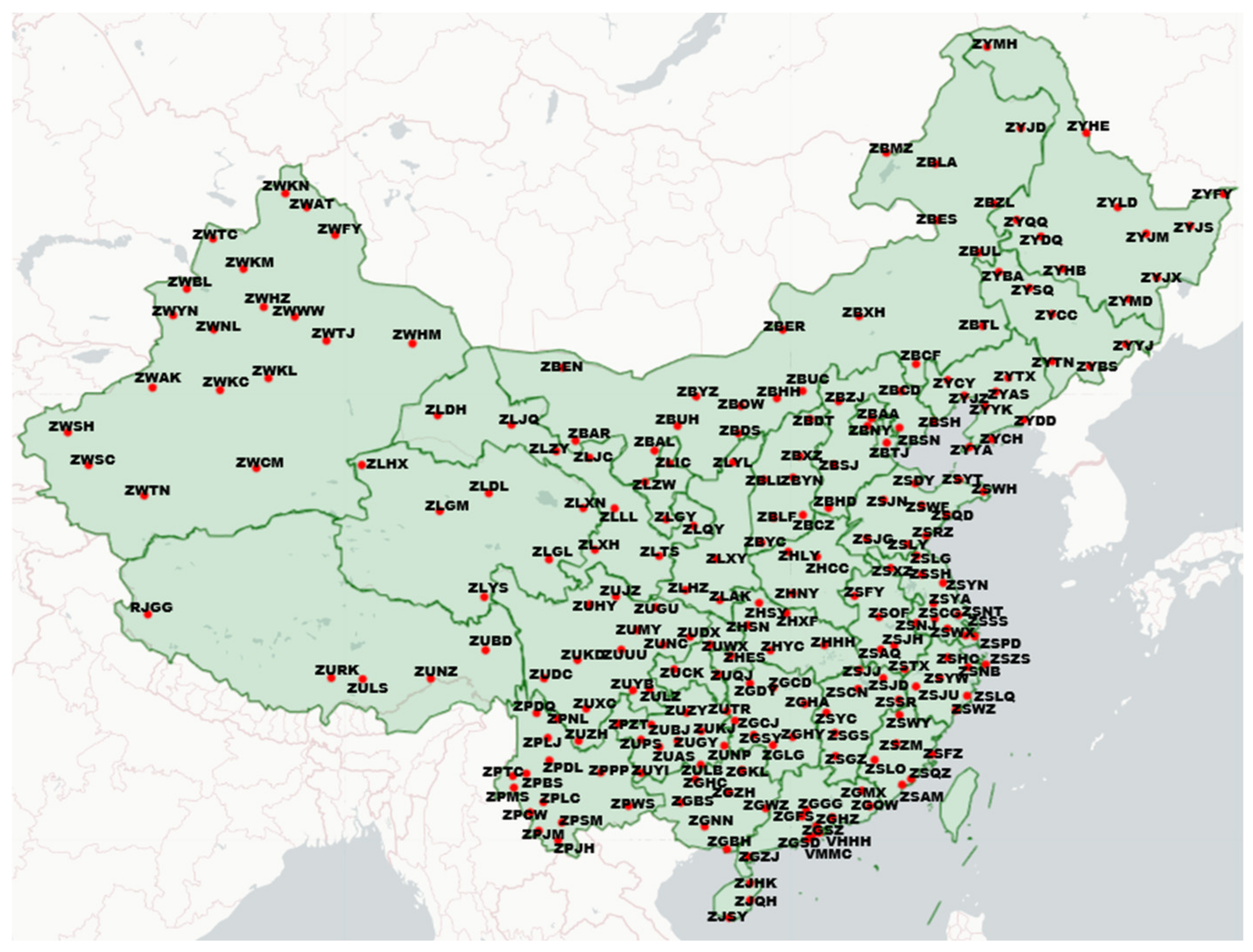
This paper takes the historical flight operation data of 219 airports in China in November and December 2018 as a case and uses the method proposed in this paper for analysis. The location distribution of each airport is shown in Figure 10. Each data attribute includes operation day, departure airport, arrival airport, planned departure time, actual departure time, planned arrival time, actual arrival time, etc. According to the planned departure time and the actual departure time, the flight that leaves the airport in advance is considered to have a delay time of 0, and the delay of a flight with a delay of more than 180 min is considered to be 180 min. At the same time, it is necessary to delete the canceled flights at each airport, because the cancelation of flights only affects the waste of related airport resources, and will not cause delays at the related airports, and the delay propagation effect on the airport network can be ignored. Generally, it takes three hours to spread to related airports after an airport is delayed. Therefore, this paper constructs delay time series with an hour as the time interval [32]. At 60 min intervals, there are 24 time periods in a day, and the average departure delay for each time period at each airport is calculated for 61 days. Each airport constitutes a delay time series with a length of 61×24 to represent the delay characteristics of the airport. A prediction model is trained using the delay time series for each airport as input data.

4.2. Sensitivity Analysis of Model Parameters

The parameters involved in the causality mining method include deep time-domain convolution prediction model parameters and causality identification parameters. The parameters of the deep temporal convolution prediction model include the learning rate, the number of training times, the number of convolution layers, and the size of the convolution kernel. The causality identification parameter includes the value of the candidate causality identification.

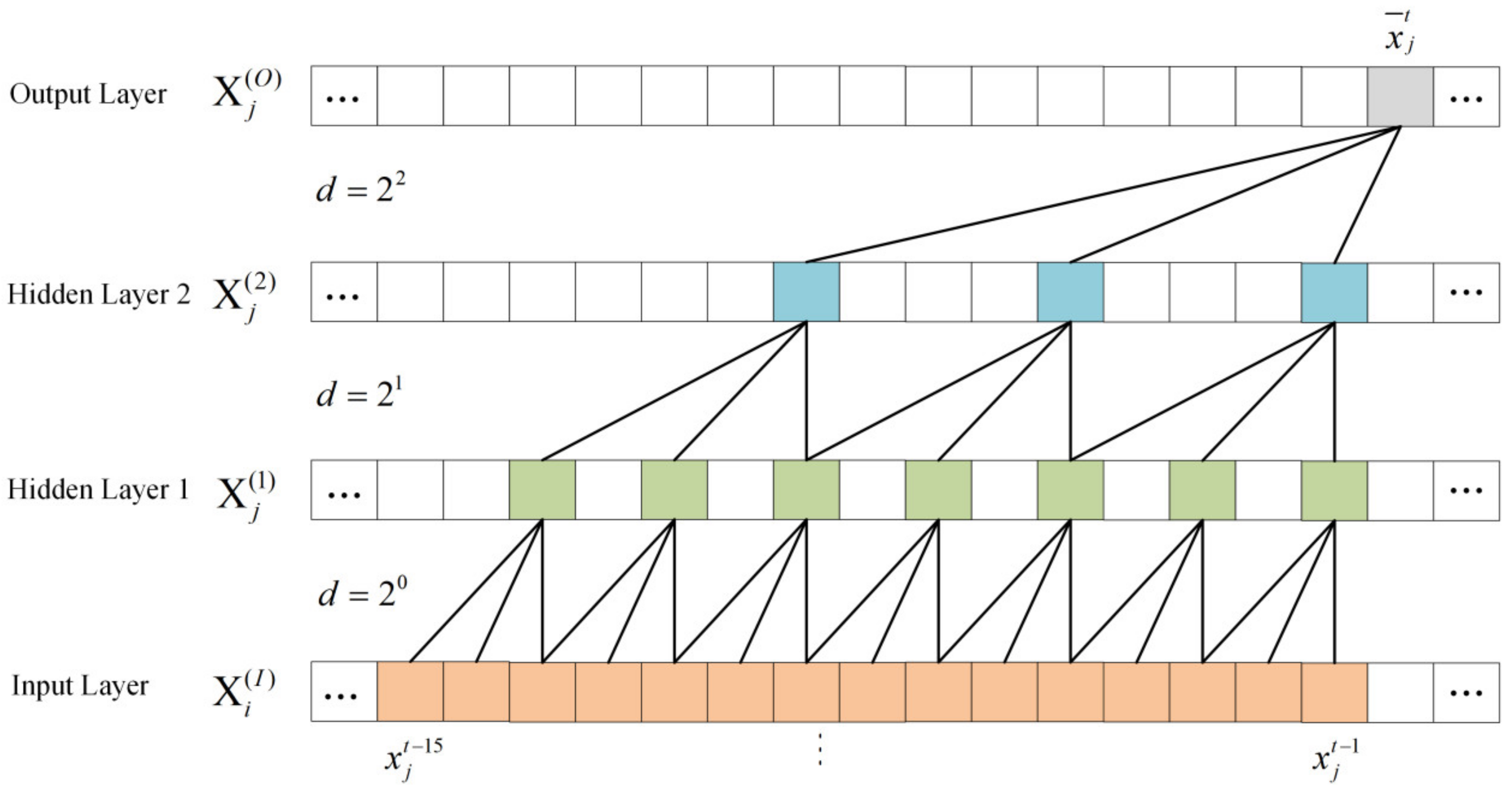
For the parameters of the deep time-domain convolution prediction model, the learning rate and the number of training times have little effect on the performance of the model and are set with general values. In this model, the learning rate is set to 0.01, and the number of training times is 500. The number of convolution layers and the size of the convolution kernel will have a great impact on the performance of the model, which depends on the size of the data, and they are the two most important parameters which are set through experiments. Considering the size of the experimental data, if the number of convolution layers exceeds 6 and the convolution kernel exceeds 8, the model will be overfitted. To this end, the number of convolutional layers is selected from the set {1,2,...,6}, and the size of the convolution kernel is selected from the set {2,...,7,8}. The performance of the models constructed with different parameter combinations is analyzed, and the parameter combination with the best model performance is selected from them. In this section, MSE error is used to measure the impact of different convolution layers and convolution kernel sizes on model performance. Experiments show that when the number of convolution layers is 6 and the size of the convolution kernel is 6, the model performance is optimal.

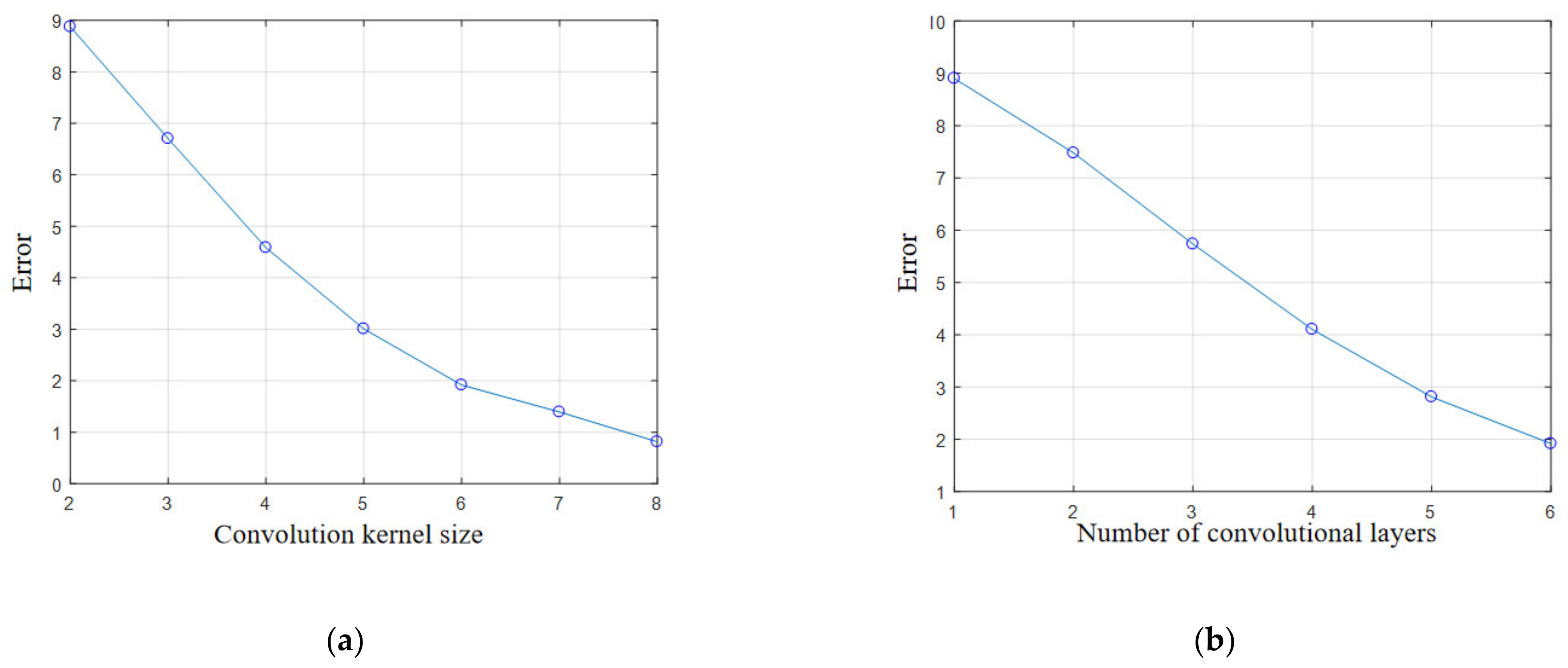
After the optimal combination of the number of convolution layers and the size of the convolution kernel is determined, the sensitivity analysis is carried out. One of the parameters is unchanged, and the influence of the other parameters on the model error is analyzed. Figure 11 is a graph of model error versus kernel size and convolution layers. As the number of convolutional layers increases and the convolution kernel becomes larger, the error becomes smaller and smaller. In Figure 11a, when the number of convolutional layers is fixed at 6 and the convolution kernel size is 2, the model prediction error is 9. The reason for the large error is that the convolution kernel is too small, so the receptive field of the input layer is too small, and there is insufficient ability to predict the target airport delay time series. When the size of the convolution kernel is 6, the model prediction error is 2. If the convolution kernel continues to increase, the rate of error decline becomes lower. In addition, if the convolution kernel is too large, it easily causes the model to be too complex and overfit and increases the operation time. In Figure 11b, when the size of the convolution kernel is 6, the effect of the change in the number of convolutional layers on the performance of the model is analyzed. When the number of convolutional layers is 1, the error is 9, and the neural network is too simple, resulting in insufficient abstraction for many input time series, and it cannot predict the target time series well. When the number of convolutional layers is 6, the error is reduced to 2, the model has sufficient ability to represent the input time series information, and the model performance is optimal.

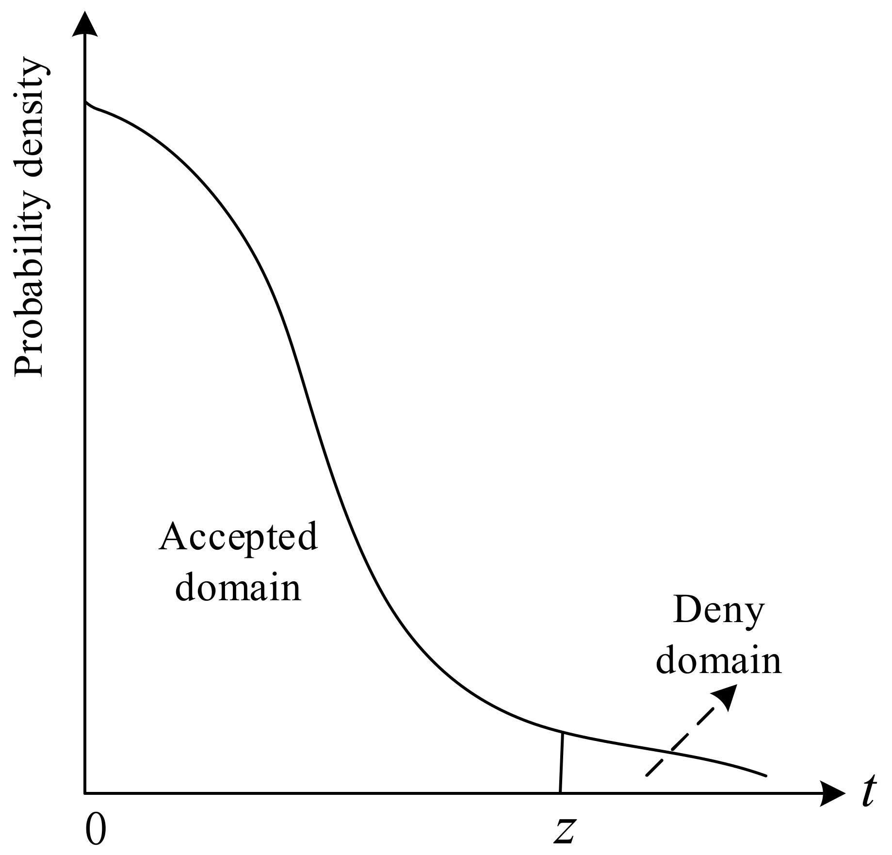
The causality identification parameters include the parameter. The parameter is related to the number of candidate causal pairs identified based on the attention score. Too many causal pairs will make the delay propagation causal network too complex, which is not conducive to airport coordination and decision-making. If the number of causal relationship pairs is too small, some important delay propagation causal relationships will be ignored, and delay propagation cannot be reduced to a large extent. Therefore, the parameter is set experimentally.

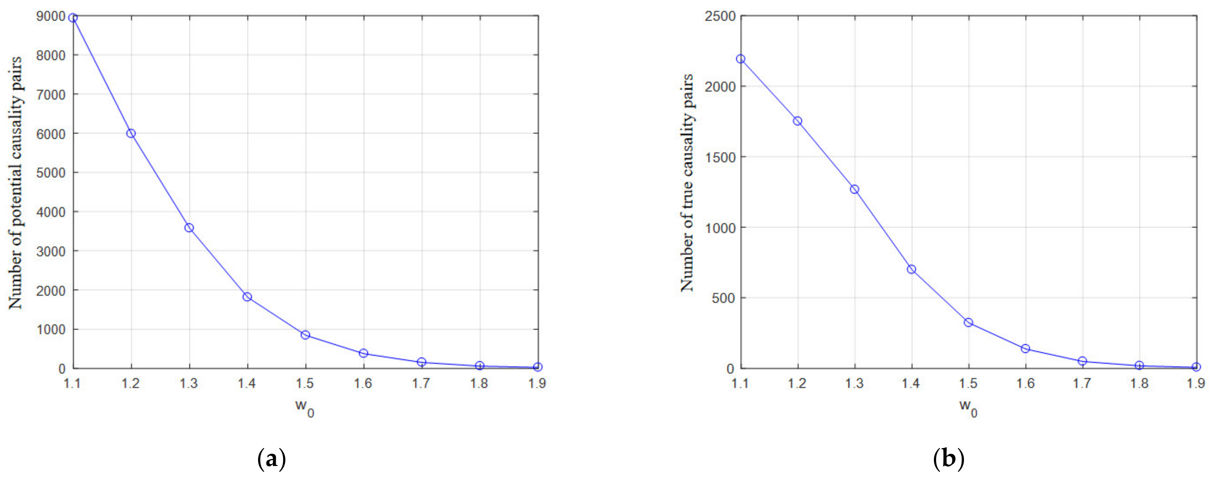
Figure 12a is a plot of the number of potential causality pairs as a function of the value of $w_0$. As the value of $w_0$ increases, the number of potential causal pairs decreases rapidly. When the $w_0$ value is 1.1, the number of potential causal relationship pairs is the largest, about 9000. When the $w_0$ value is greater than 1.7, the number of potential causal relationship pairs is almost 0, indicating that there is no delay propagation relationship between airports. The identification of potential causal relationships is based on the attention factor score, and the attention factor score does not change after the prediction model training is completed. It is considered that the airport with an attention factor score greater than the $w_0$ value is the candidate cause set of the target airport, so when the $w_0$ value is the smallest, the number of candidate causal relations is the largest, and the candidate causal relation set with the large $w_0$ value is included. In addition, most airports have attention factor scores of 1.1–1.4, so when the $w_0$ value is greater than 1.4, the number of potential causalities declines more slowly. Figure 12b is a line graph of the number of true causal airport pairs as a function of the value of $w_0$. As $w_0$ increases, the true causality has a decreasing trend to the quantity. When W is 1.1, the number of true causality pairs is the largest. When $w_0$ is greater than 1.7, the number of true causal relationship pairs is almost 0, that is, there is no delay propagation relationship between airports. In order to facilitate the decision-making of airport control, $w_0$ is set to 1.3 here.

4.3. Result Analysis

If delays at one airport lead to delays at another airport, the two airports are connected to build a delay causality network diagram. The following is a comparative analysis of the causal relationship network, the causal relationship network with an in-degree greater than 10, and the causal relationship network with an out-degree greater than 10.

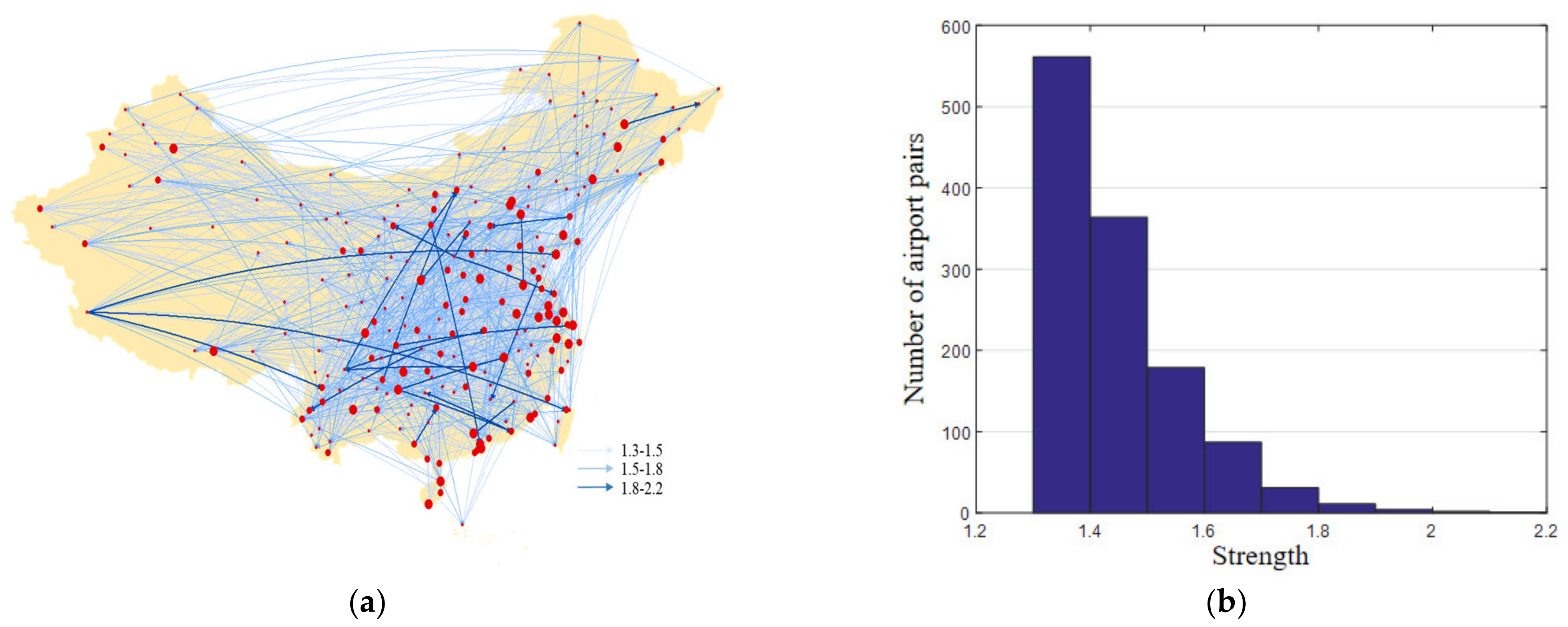
Figure 13a is a directed network graph of delay propagation causality at Chinese airports, containing 219 nodes and 1266 edges. Larger nodes indicate more severe airport delays. A directed edge indicates that there is a causal relationship between the two airports, from the airport where the delay occurred to the airport affected by it. The darker the color of the edge, the greater the strength of the causal relationship between the two airports. The strength of the causal relationship indicates the credibility of the causal relationship between the two airports. The greater the strength, the greater the credibility of the causal relationship. There are 925 directed edges with a causal relationship strength of 1.3–1.5, 297 directed edges with a strength of 1.5–1.8, and 18 directed edges with a strength of 1.8–2.2. Directed edges with strengths greater than 1.8 are much smaller than directed edges with strengths less than 1.8. This is because it is rarely the case that delays at one airport are definitely caused by delays at another airport, often due to a variety of reasons such as weather and airlines. Among the 18 sides with the greatest intensity, Yulin Yuyang Airport (ZLYL) and Xichang Qingshan Airport (ZUXC) caused delays at many airports, ZLYL’s delays caused delays at 38 other airports, and ZUXC’s delays caused delays at another 27 airports. ZLYL has an average of 29 departure flights per day, and ZUXC has an average of 11 departure flights per day, which is far less than the average daily departure flight volume of Beijing Capital International Airport (ZBAA) of 860. It can be seen that airports with small flight volumes are more likely to affect other airports and cause delays. Figure 13b is a histogram that further refines the number of edges corresponding to different causality strengths, with a step size of 0.1, and statistical strengths for causal relationship pairs in each interval between 1.3 and 2.3. There are 561 pairs of airports with strengths 1.3–1.4, the most causal pairs. In addition, the greater the strength, the smaller the number of causality pairs. The number of sides with a strength of 1.9–2 is almost equal to the number of sides with a strength of 2–2.1. The number of edges with strength from 2.1–2.2 is only one.

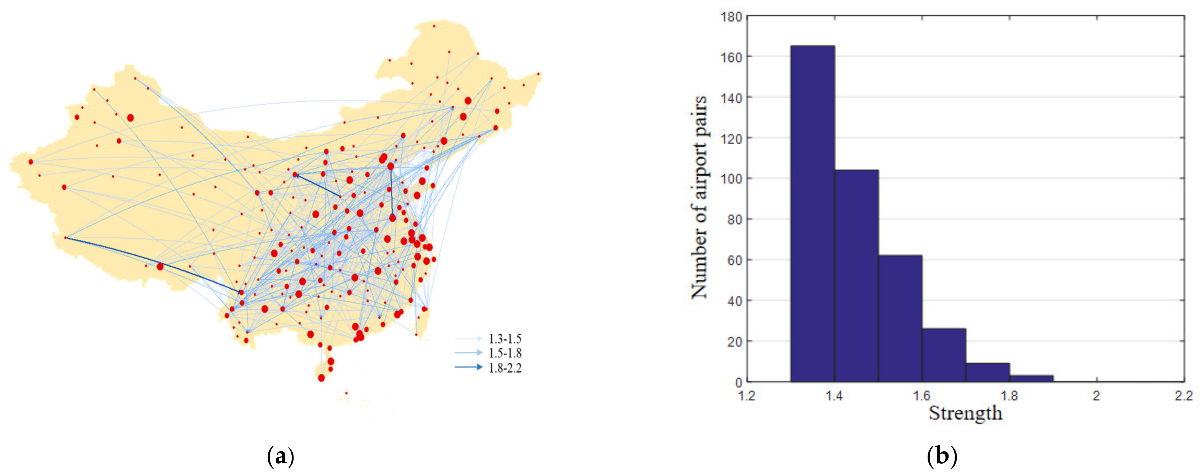
Figure 14a is a causal network diagram with an in-degree greater than 10. There are 32 airports with an in-degree greater than 10, and 369 causal pairs. The analysis found that airports with small delays are more likely to be affected by other airports. Figure 14b is a histogram of the number of edges corresponding to different intensities in a causal network with an in-degree greater than 10, showing the same law as Figure 13b. 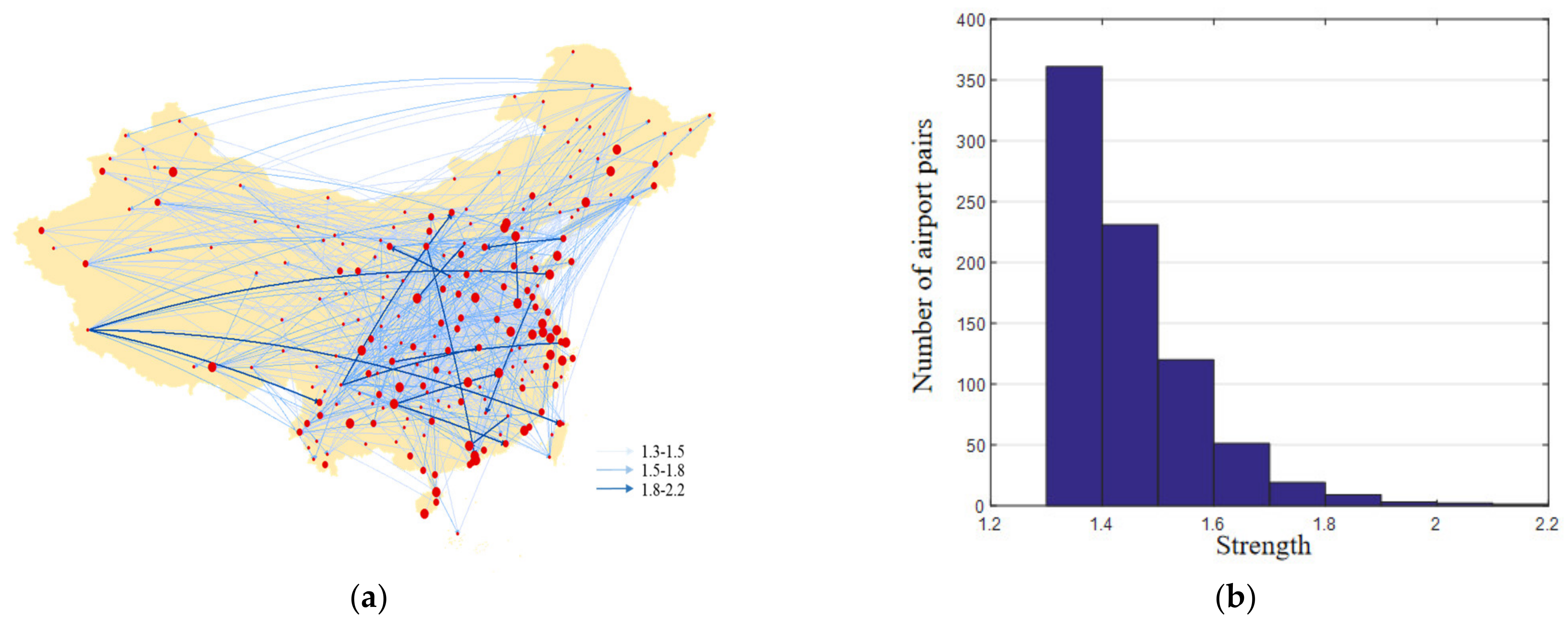Figure 15a is a causal relationship network diagram with an out-degree greater than 10, in which there are 47 airports with an out-degree greater than 10, and 797 causal relationship pairs. In a strong causal relationship, flights with moderate delays are more likely to affect other airports. Figure 15b is a histogram of the number of sides corresponding to different intensities in a causal relationship with an out-degree greater than 10, showing the same law as Figure 13.

4.4. Topological Property Analysis

Topological properties are properties that remain unchanged after a graph changes shape continuously. The topological property analysis of the airport delay propagation causality network is helpful to understand the invariance of the entire delay propagation causality network.

The degree of a node is an important method to describe the structure of a complex network, it represents the number of edges connected to the node in the network. The causal relationship network in this paper belongs to the directed graph network, and the degree is divided into in-degree and out-degree. This experiment discusses the in-degree distribution and out-degree distribution of the network and analyzes how many other airports’ delays will be affected by the delay of one airport. 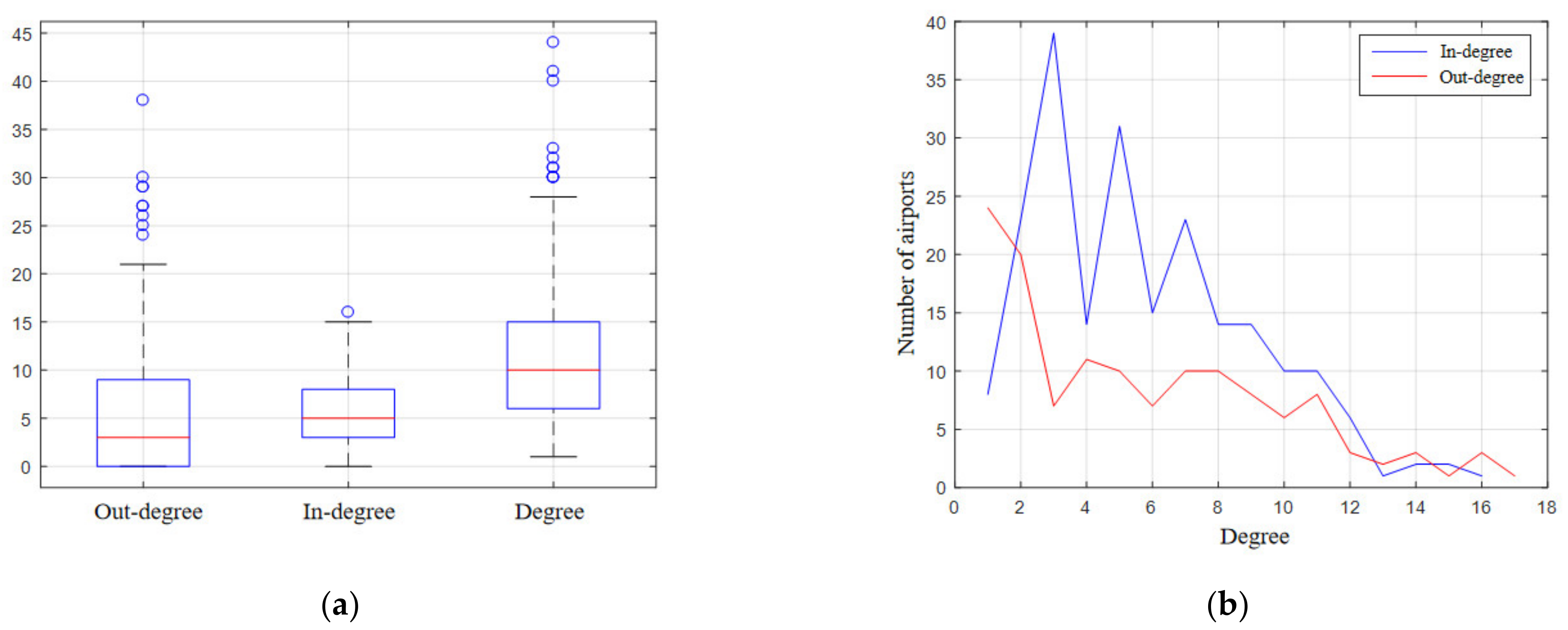Figure 16a shows the distribution of in-degree, out-degree, and degree of an airport with a boxplot. The degree of an airport is equal to the sum of out-degree and in-degree. The average in-degree is equal to the average out-degree, which is 5.74, indicating that an airport will be affected by another six airports on average, and will also affect another six airports on average. For the in-degree, the minimum value is 0, indicating that the delays at these airports are not caused by the delays of other airports, but are caused by the weather and other reasons. Most airports have in-degree values of 3 to 8. Although the airport will be affected by other airports, it will not be affected by too many other airports’ delays (the number of other airports will not be too large). The maximum in-degree value of an airport is 16. This airport is Baoshan Yunrui Airport (ZPBS). The airport has an average daily departure flight of 16. The same conclusion as in Section 4.3 is obtained: an airport with a small flight volume is easily affected by many other airports. For out-degrees, 25% of the airports have out-degree values of 0, indicating that delays at these airports will not affect delays at other airports. Except for Yulin Yuyang Airport (ZLYL), the out-degree value is 38, which affects many airports. Seventy-five percent of the airports have an out-degree value below 9, which will only affect the normal operation of the airport that is most closely related to it.

The maximum in-degree in Figure 16a is 16. To compare the similarities and differences in the number of airports when the in-degree and out-degree are equal, Figure 16b plots the number of airports in the network with degrees from 1 to 17 in the entire causal network. There are eight airports with an in-degree of 1, and 24 airports with an out-degree of 1. The number of airports decreases with the increase in in-degree and out-degree. When the in-degree and out-degree take the same value of less than 12, the number of in-degree airports is greater than the number of out-degree airports. Especially when the in-degree and out-degree values are 3, the difference in the number of airports is 32. When the in-degree and out-degree take the same value greater than 13, the number of airports is almost the same, with an average of 3, and the number of airports that affect many other airports and are affected by delays of many other airports is small. 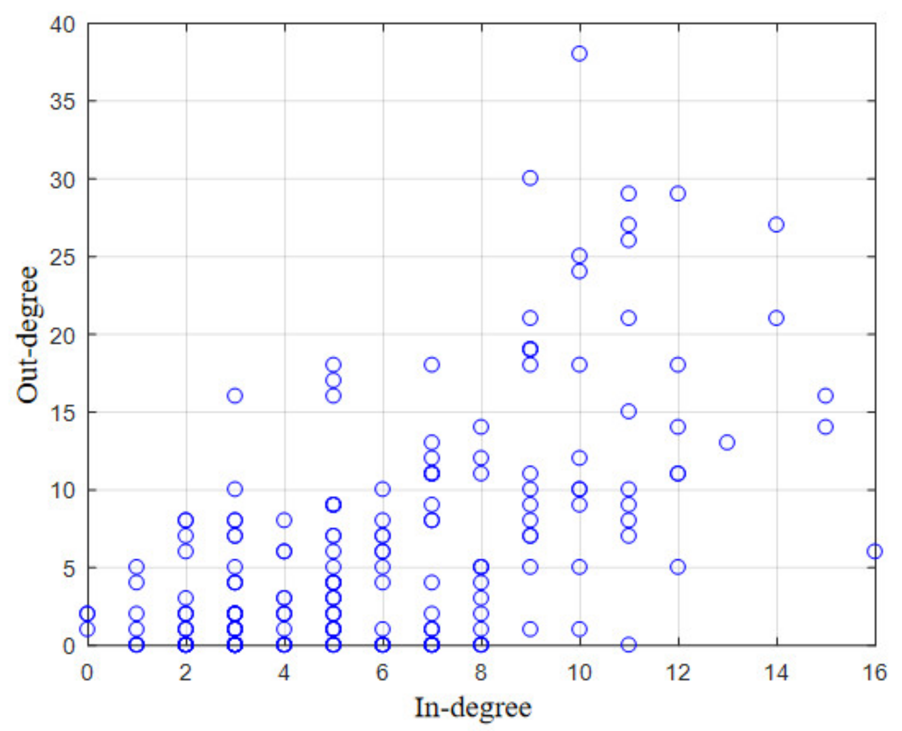Figure 17 is a scatterplot of the in-degree and out-degree relationships for each airport. The airport with the largest in-degree is Baoshan Yunrui Airport, but the corresponding out-degree is not the largest. The airport with the largest out-degree has an in-degree of 10. However, on the whole, airports with large in-degrees generally have large out-degrees.

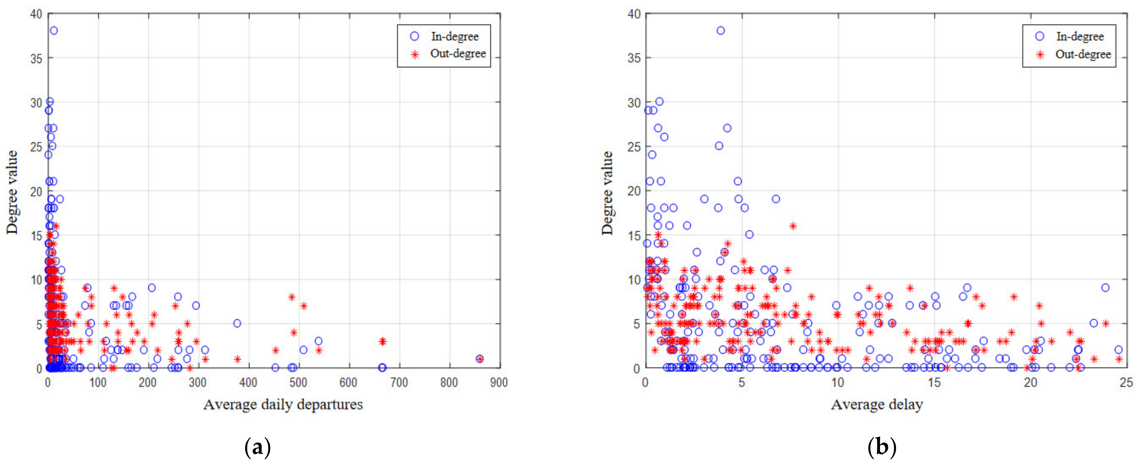
Figure 18a shows the relationship between the average daily departure flight volume and degree, that is, the delay caused by airports with different flight volumes is affected by how many airports are delayed and how many airports are affected by delays. There are 6 airports with a small number of flights, but the out-degree is greater than 25. There are 8 airports with a large number of flights, but the in-degree and out-degree are small. In general, most airports have 0–300 departure flights, and 0–10 inbound and outbound flights. These airports are susceptible to being influenced by other airports, and at the same time, they are also easily influenced by other airports. Airports with more than 300 flights have small in-degrees and are not easily affected by other airports. They have a strong ability to absorb delays. From here, it can also be seen that the airport with the smallest number of flights has the largest in-degree and out-degree. Figure 18b shows the relationship between the average delay of departure and the degree value for each airport. The relationship between airport delay level and out-degree value is similar to the relationship between airport flight volume and out-degree value. The smaller the average delay time, the easier it is to affect other airports. There is no obvious relationship between the in-degree and the average delay time of the airport. It does not mean that the airport with a smaller delay is more easily affected by other airports, and it does not mean that the airport with greater delay is more easily affected by other airports.

Table 2. Delay propagation causality network metric values.

Metrics	Value
connection density (ld)	0.0266
interaction parameter	0.0018
clustering coefficient	0.1405

gives the values of connection density, interaction parameter, aggregation coefficient, and connection density $l_d$ to represent the degree of tightness of network connection, which is defined as the ratio of the number of edges of the network to the number of possible edges of all nodes, and the value range is between [0, 1]. The larger the value of $l_d$, the tighter the network connection is, and the more easily the delay propagates in the network. The connection density of this causal relationship network is 0.0266, which is related to the choice of model parameters so that the network connection is not tight, and the delay propagation can be blocked by certain measures in the airport network. The interaction parameter indicates whether the delay propagation between airport pairs is bidirectional. Delays at the airport $i$ will affect delays at airport j, and delays at airport j will also affect delays at the airport $i$. The interaction parameters were calculated using the method provided in [31]. The average $\overline{R}$ of 1000 random networks with the same number of nodes and edges generated by the network randomization technique is 0.17. Compared with this value, the interaction parameter of the causal network is much smaller than $\overline{R}$, so the number of airport pairs in the network where delays propagate and influence each other is considered to be very small. If the delay of one airport leads to the delay of other airports, then other airports are called neighbor airports. The ratio of the actual causal relationship between these neighboring airports and the possible causal relationship is called the aggregation coefficient, which reflects the aggregation degree of the airport. For directed networks, the clustering coefficient is calculated using the method provided in [17,19]. The overall clustering coefficient of this causal network is 0.1405, which is larger than that of the random network (0.092). It shows the clustering trend among airports in the delay causality network, and delay causality often exists between the other two airports affected by the delay of one airport.

5. Conclusions

This paper proposes a deep time series convolutional neural network causality discovery method, which considers the entire airport network at the same time, and correctly discovers the delay propagation causality of the airport network. This method includes two parts: a deep time series convolutional network prediction model and causal relationship analysis. The deep time series convolutional network prediction model takes the delay time series of all airports as input and the time series of a single target airport as output and introduces an attention mechanism to better discover and explain the contribution of each input airport to the target airport. The causal relationship analysis includes the potential causality analysis based on the attention mechanism, and then from the potential causality, the direct causality is verified based on the permutation importance test. According to the verified causal relationship, the network is constructed, the performance and topology properties of the network are analyzed, and the delay propagation mechanism of the airport network is studied.

Applying this method to the research on the delay propagation mechanism of China’s airport network, an airport is affected by six airports on average, and it will also affect six airports at the same time. Airports with small flight volumes and airports with moderate delays are more likely to affect other airports, and airports with small delays are more likely to be affected by other airports. The research results of this paper can provide a theoretical basis for delay control. This paper takes the Chinese airport network as a case. Further research will try to apply the method in this paper to other countries to compare whether there are differences in airport delay networks in different countries.

References

1. Chen, C.; Li, C.; Chen, J.; Wang, C. VFDP: Visual Analysis of Flight Delay and Propagation on a Geographical Map. IEEE Trans. Intell. Transp. Syst. 2022, 23, 3510–3521. [Google Scholar] [CrossRef]
2. Eufrásio, A.B.R.; Eller, R.A.G.; Oliveira, A.V.M. Are on-time performance statistics worthless? An empirical study of the flight scheduling strategies of Brazilian airlines. Transp. Res. Part E Logist. Transp. Rev. 2021, 145, 102186. [Google Scholar] [CrossRef]
3. Miranda, V.A.P.; Oliveira, A.V.M. Airport slots and the internalization of congestion by airlines: An empirical model of integrated flight disruption management in Brazil. Transp. Res. Part A Policy Pract. 2018, 116, 201–219. [Google Scholar] [CrossRef]
4. Churchill, A.M.; Lovell, D.J.; Ball, M.O. Flight delay propagation impact on strategic air traffic flow management. Transp. Res. Rec. 2010, 2177, 105–113. [Google Scholar] [CrossRef]
5. Montoya, J.; Rathinam, S.; Wood, Z. Multiobjective Departure Runway Scheduling Using Dynamic Programming. IEEE Trans. Intell. Transp. Syst. 2014, 15, 399–413. [Google Scholar] [CrossRef]
6. Zeng, W.; Ren, Y.; Wei, W.; Yang, Z. A data-driven flight schedule optimization model considering the uncertainty of operational displacement. Comput. Oper. Res. 2021, 133, 105328. [Google Scholar] [CrossRef]
7. Bureau of Transportation Statistics. Understanding the Reporting of Causes of Flight Delays and Cancellations; Bureau of Transportation Statistics: Washington, DC, USA, 2019.
8. Baspinar, B.; Koyuncu, E. A Data-Driven Air Transportation Delay Propagation Model Using Epidemic Process Models. Int. J. Aerosp. Eng. 2016, 2016 Pt 2, 4836260. [Google Scholar] [CrossRef]
9. Kafle, N.; Zhou, B. Modeling flight delay propagation: A new analytical-econometric approach. Transp. Res. Part B Methodol. 2016, 93, 520–542. [Google Scholar] [CrossRef]
10. Pyrgiotis, N.; Malone, K.M.; Odoni, A. Modelling delay propagation within an airport network. Transp. Res. Part C Emerg. Technol. 2013, 27, 60–75. [Google Scholar] [CrossRef]
11. Wu, W.; Zhang, H.; Feng, T.; Witlox, F. A Network Modelling Approach to Flight Delay Propagation: Some Empirical Evidence from China. Sustainability 2019, 11, 4408. [Google Scholar] [CrossRef]
12. Bendinelli, W.E.; Bettini, H.F.A.J.; Oliveira, A.V.M. Airline delays, congestion internalization and non-price spillover effects of low cost carrier entry. Transp. Res. Part A Policy Pract. 2016, 85, 39–52. [Google Scholar] [CrossRef]
13. Fleurquin, P.; Ramasco, J.J.; Eguiluz, V.M. Characterization of Delay Propagation in the US Air-Transportation Network. Transp. J. 2014, 53, 330–344. [Google Scholar] [CrossRef] [Green Version]
14. Wu, W.; Wu, C.-L. Enhanced delay propagation tree model with Bayesian Network for modelling flight delay propagation. Transp. Plan. Technol. 2018, 41, 319–335. [Google Scholar] [CrossRef]
15. Zanin, M.; Belkoura, S.; Zhu, Y. Network analysis of Chinese air transport delay propagation. Chin. J. Aeronaut. 2017, 30, 491–499. [Google Scholar] [CrossRef]
16. AhmadBeygi, S.; Cohn, A.; Guan, Y.; Belobaba, P. Analysis of the potential for delay propagation in passenger airline networks. J. Air Transp. Manag. 2008, 14, 221–236. [Google Scholar] [CrossRef] [Green Version]
17. Hsu, C.-I.; Hsu, C.-C.; Li, H.-C. Flight-delay propagation, allowing for behavioural response. Int. J. Crit. Infrastruct. 2007, 3, 301–326. [Google Scholar] [CrossRef]
18. Zhang, H.; Wu, W.; Zhang, S.; Witlox, F. Simulation Analysis on Flight Delay Propagation under Different Network Configurations. IEEE Access 2020, 8, 103236–103244. [Google Scholar] [CrossRef]
19. Ciruelos, C.; Arranz, A.; Etxebarria, I.; Peces, S.; Campanelli, B.; Fleurquin, P.; Eguiluz, V.M.; Ramasco, J.J. Modelling Delay Propagation Trees for Scheduled Flights. In Proceedings of the Eleventh USA/Europe Air Traffic Management Research and Development Seminar (ATM2015), Lisbon, Portugal, 23–26 June 2015. [Google Scholar]
20. Liu, Y.J.; Cao, W.D.; Song, M. Estimation of Arrival Flight Delay and Delay Propagation in a Busy Hub-Airport. In Proceedings of the Fourth International Conference on Natural Computation, Jinan, China, 18–20 October 2008. [Google Scholar]
21. Fleurquin, P.; Ramasco, J.J.; Eguiluz, V.M. Data-driven modeling of systemic delay propagation under severe meteorological conditions. In Proceedings of the 10th USA/Europe Air Traffic Management Research and Development Seminar, ATM 2013, EUROCONTROL, Chicago, IL, USA, 10–13 June 2013. [Google Scholar]
22. Fleurquin, P.; Ramasco, J.; Eguiluz, V. Systemic delay propagation in the US airport network. Sci. Rep. 2013, 3, 1159. [Google Scholar] [CrossRef] [Green Version]
23. Campanelli, B.; Fleurquin, P.; Arranz, A.; Etxebarria, I.; Ciruelos, C.; Eguíluz, V.M.; Ramasco, J.J. Comparing the modeling of delay propagation in the US and European air traffic networks. J. Air Transp. Manag. 2016, 56, 12–18. [Google Scholar] [CrossRef]
24. Wu, C.-L.; Law, K. Modelling the delay propagation effects of multiple resource connections in an airline network using a Bayesian network model. Transp. Res. Part E Logist. Transp. Rev. 2019, 122, 62–77. [Google Scholar] [CrossRef]
25. Dai, X.; Hu, M.; Tian, W.; Liu, H. Modeling Congestion Propagation in Multistage Schedule within an Airport Network. J. Adv. Transp. 2018, 2018 Pt 5, 6814348. [Google Scholar] [CrossRef]
26. Wu, Q.; Hu, M.; Ma, X.; Wang, Y.; Cong, W.; Delahaye, D. Modeling Flight Delay Propagation in Airport and Airspace Network. In Proceedings of the 2018 IEEE International Conference on Intelligent Transportation Systems (ITSC), Maui, HI, USA, 4–7 November 2018. [Google Scholar]
27. AhmadBeygi, S.; Cohn, A.; Lapp, M. Decreasing airline delay propagation by re-allocating scheduled slack. IIE Trans. 2010, 42, 478–489. [Google Scholar] [CrossRef] [Green Version]
28. Kim, M.; Park, S. Airport and route classification by modelling flight delay propagation. J. Air Transp. Manag. 2021, 93, 102045. [Google Scholar] [CrossRef]
29. Ivanov, N.; Netjasov, F.; Jovanović, R.; Starita, S.; Strauss, A. Air Traffic Flow Management slot allocation to minimize propagated delay and improve airport slot adherence. Transp. Res. Part A Policy Pract. 2017, 95, 183–197. [Google Scholar] [CrossRef]
30. Granger, C.W.J. Investigating causal relations by econometric models and cross-spectral methods. Econom. J. Econom. Soc. 1969, 37, 424–438. [Google Scholar] [CrossRef]
31. Du, W.B.; Zhang, M.Y.; Zhang, Y.; Cao, X.B.; Zhang, J. Delay Causality Network in Air Transport Systems. Transp. Res. Part E Logist. Transp. Rev. 2018, 118, 466–476. [Google Scholar] [CrossRef]
32. Zhang, M.; Zhou, X.; Zhang, Y.; Sun, L.; Dun, M.; Du, W.; Cao, X. Propagation Index on Airport Delays. Transp. Res. Rec. 2019, 2673, 536–543. [Google Scholar] [CrossRef]
33. Xu, C.; Ji, J.; Liu, P. The station-free sharing bike demand forecasting with a deep learning approach and large-scale datasets. Transp. Res. Part C Emerg. Technol. 2018, 95, 47–60. [Google Scholar] [CrossRef]
34. Yang, B.; Sun, S.; Li, J.; Lin, X.; Tian, Y. Traffic flow prediction using LSTM with feature enhancement. Neurocomputing 2019, 332, 320–327. [Google Scholar] [CrossRef]
35. Zheng, Z.; Chen, W.; Wu, X.; Chen, P.C.; Liu, J. LSTM network: A deep learning approach for short-term traffic forecast. IET Intell. Transp. Syst. 2017, 11, 68–75. [Google Scholar]
36. Li, X.; Peng, L.; Yao, X.; Cui, S.; Hu, Y.; You, C.; Chi, T. Long short-term memory neural network for air pollutant concentration predictions: Method development and evaluation. Environ. Pollut. 2017, 231, 997–1004. [Google Scholar] [CrossRef]
37. Verma, I.; Ahuja, R.; Meisheri, H.; Dey, L. Air Pollutant Severity Prediction Using Bi-Directional LSTM Network. In Proceedings of the 2018 IEEE/WIC/ACM International Conference on Web Intelligence (WI), Santiago, Chile, 3–6 December 2018. [Google Scholar]
38. Cao, J.; Li, Z.; Li, J. Financial time series forecasting model based on CEEMDAN and LSTM. Phys. A Stat. Mech. Its Appl. 2019, 519, 127–139. [Google Scholar] [CrossRef]
39. Fischer, T.; Krauss, C. Deep learning with long short-term memory networks for financial market predictions. Eur. J. Oper. Res. 2018, 270, 654–669. [Google Scholar] [CrossRef] [Green Version]
40. Gao, Y.; Phillips, J.M.; Zheng, Y.; Min, R.; Fletcher, P.T.; Gerig, G. Fully convolutional structured LSTM networks for joint 4D medical image segmentation. In Proceedings of the 2018 IEEE 15th International Symposium on Biomedical Imaging (ISBI 2018), Washington, DC, USA, 4–7 April 2018. [Google Scholar]
41. Hu, J.; Guo, C.; Yang, B.; Jensen, C.S. Stochastic Weight Completion for Road Networks Using Graph Convolutional Networks. In Proceedings of the 2019 IEEE 35th International Conference on Data Engineering (ICDE), Macau, China, 8–11 April 2019. [Google Scholar]
42. Louizos, C.; Shalit, U.; Mooij, J.M.; Sontag, D.; Zemel, R.; Welling, M. Causal Effect Inference with Deep Latent-Variable Models. Adv. Neural Inf. Process. Syst. 2017, 30, 1–11. [Google Scholar]
43. Goudet, O.; Kalainathan, D.; Caillou, P.; Guyon, I.; Lopez-Paz, D.; Sebag, M. Causal Generative Neural Networks. arXiv 2017, arXiv:1711.08936. [Google Scholar]
44. Kalainathan, D.; Goudet, O.; Guyon, I.; Lopez-Paz, D.; Sebag, M. Structural Agnostic Modeling: Adversarial Learning of Causal Graphs. arXiv 2018, arXiv:1803.04929. [Google Scholar]
45. Eichler, M. Causal Inference in Time Series Analysis; John Wiley & Sons, Ltd.: Hoboken, NJ, USA, 2012. [Google Scholar]
46. Xiong, J.; Hansen, M. Value of flight cancellation and cancellation decision modeling: Ground delay program postoperation study. Transp. Res. Rec. 2009, 2106, 83–89. [Google Scholar] [CrossRef]
47. Chollet, F. Xception: Deep learning with depthwise separable convolutions. In Proceedings of the IEEE Conference on Computer Vision and Pattern Recognition, Honolulu, HI, USA, 21–26 July 2017. [Google Scholar]
Figure 1. Airport delay propagation causality. (a) No causation; (b) Direct causation; (c) Indirect causation; (d) Both direct and indirect causation.
Applsci 12 10433 g001
Figure 2. Direct causal network of airport delay propagation. The delay of airport v i is transmitted unidirectionally to airport v 1 , while there is a bidirectional delay propagation relationship between v i and v j .
Applsci 12 10433 g002
Figure 3. Diagram of confounding causality. Airport A, airport B, and airport C are the “cause” airports of airport Z.
Applsci 12 10433 g003
Figure 4. The general idea of causality mining of airport delay propagation.
Applsci 12 10433 g004
Figure 5. The DTCN prediction model architecture based on the attention mechanism.
Applsci 12 10433 g005
Figure 6. Single-channel depthwise convolution.
Applsci 12 10433 g006
Figure 7. Depthwise separable convolution.
Applsci 12 10433 g007
Figure 8. One-tailed t-distribution.
Applsci 12 10433 g008
Figure 9. Flow chart of direct causality verification based on propagation delay analysis.
Applsci 12 10433 g009
Figure 10. Location distribution map of 219 major airports in China.
Applsci 12 10433 g010
Figure 11. Influence of the number of convolution layers and the size of convolution kernel on model error. (a) The influence of the size of the convolution kernel, (b) the number of convolutional layers on the model error.
Applsci 12 10433 g011
Figure 12. Graph of the number of candidate causality pairs and true causality pairs as a function of w 0 . (a) The relationship between the number of potential causality pairs and w 0 ; (b) the relationship between the number of true causality pairs and w 0 .
Applsci 12 10433 g012
Figure 13. Real delay propagation causal network diagram. (a) Causality network (b) Number of airport pairs with different strength.
Applsci 12 10433 g013
Figure 14. Delayed propagation causality network with in-degree greater than 10. (a) Causality network (b) Number of airport pairs with different strength.
Applsci 12 10433 g014
Figure 15. Delayed propagation causality network with an out-degree greater than 10. (a) Causality network (b) Number of airport pairs with different strength.
Applsci 12 10433 g015
Figure 16. Degree distribution. (a) Box plot of out-degree, in-degree, and degree, (b) Number of airports with different in-degree and out-degree.
Applsci 12 10433 g016
Figure 17. Relationship between airport in-degree and out-degree.
Applsci 12 10433 g017
Figure 18. Relationship between 20 degrees and departure flight volume and average delay time. (a) Degree value vs average daily departures, (b) Degree value vs average dalsy.
Applsci 12 10433 g018