
Passive Array-Invariant-Based Localization for a Small Horizontal Array Using Two-Dimensional Deconvolution

1
Institute of Acoustics, Chinese Academy of Sciences, Beijing 100190, China
2
Key Laboratory of Science and Technology on Advanced Underwater Acoustic Signal Processing, Chinese Academy of Sciences, Beijing 100190, China
*
Author to whom correspondence should be addressed.
Appl. Sci. 2022, 12(18), 9356; https://doi.org/10.3390/app12189356
Submission received: 25 July 2022
/
Revised: 5 September 2022
/
Accepted: 13 September 2022
/
Published: 18 September 2022
(This article belongs to the Special Issue Underwater Acoustic Signal Processing)
Abstract
:Recently, the array-invariant method was proposed to passively localize sources of opportunity in shallow water. It exploits multiple arrivals which are different in terms of beam angle and travel time. Conventional plane-wave beamforming in the existing array-invariant method is used to obtain beam-time migration. The resolution capability of conventional plane-wave beamforming is determined by array aperture, which, however, limits the localization accuracy of the existing array-invariant method. To improve the localization accuracy, this study proposes the use of two-dimensional (2D) deconvolution to obtain a better beam-time migration than in conventional plane-wave beamforming. Our simulation with a small horizontal array showed that the range estimation error of the proposed array-invariant method based on 2D deconvolution was only one-third of that of the existing method. The experiment also demonstrated the validity of our proposed method.
1. Introduction
Underwater source localization is a hot topic in underwater acoustic signal processing [1,2,3,4,5,6,7,8]. The array-invariant method, based on the dispersion characteristics of wideband signals in waveguides, was proposed by Lee and Makris in 2006 for shallow sea source localization [2]. With the development of blind deconvolution [3,4,5], the array-invariant method has been successfully applied to passively localize surface ships or submerged sources, using a vertical [6,7,8,9] or horizontal [10,11] array without knowledge of the ocean environment. The blind deconvolution method extracts the Green’s function, namely the channel impulse response, between a source of opportunity (e.g., ship) and an array. Subsequently, conventional plane-wave beamforming is employed to obtain the beam-time migration of the Green’s function. Finally, the array-invariant method estimates the source range from the beam-time migration using the least-squares approach [2,11].
Following the steps of the existing array-invariant method, it can be found that beam-time migration plays a key role in the source–range estimation. To date, only conventional plane-wave beamforming has been utilized to obtain the beam-time migration in localization applications [7,8,9,11]. However, the resolution capability of conventional plane-wave beamforming is determined by the array aperture, which influences the localization accuracy of the existing array-invariant method, especially when using a small horizontal array. The relatively wide beam-time migration should be one of the main reasons causing the source–range estimation error of the existing array-invariant method. This study attempts to decrease the source–range estimation error by obtaining better beam-time migration by using two-dimensional (2D) deconvolution.
In this paper, with some mathematical derivations, we employ frequency-domain beamforming to process the extracted Green’s function to obtain the beam-time migration, which is expressed as a 2D convolution. Based on the deduced 2D convolution expression, we propose a 2D deconvolution method to deconvolve the beam-time migration obtained with conventional plane-wave beamforming to obtain the high-resolution beam-time migration. The more accurate source range can thus be estimated from the high-resolution beam-time migration. The existing array-invariant method [11] involving blind deconvolution and conventional plane-wave beamforming is referred to as the reference method in this study. The simulation with a small horizontal array in shallow water shows that the source–range estimation error of our proposed method based on the 2D deconvolution is only one third of that of the reference method. The experiment with a small horizontal array in the Yellow Sea of China also proves the validity of our proposed method. Additionally, the results in this study also demonstrate that the wide beam-time migration obtained with conventional plane-wave beamforming in the array-invariant method is one of the main reasons behind source–range estimation errors.
This brief report is organized as follows: Section 2 describes the Green’s function and blind deconvolution for the horizontal array. In Section 3.1, conventional plane-wave beamforming is reviewed. In Section 3.2, the 2D deconvolution method is proposed to deconvolve the beam-time migration obtained with conventional plane-wave beamforming. The 2D deconvolution method can obtain high-resolution beam-time migration. The simulation and the experiment are described in Section 4 and Section 5, respectively. The simulation and the experiment demonstrate the validity of our proposed method. Finally, our conclusion is provided in Section 6.
2. Extracting Green’s Function
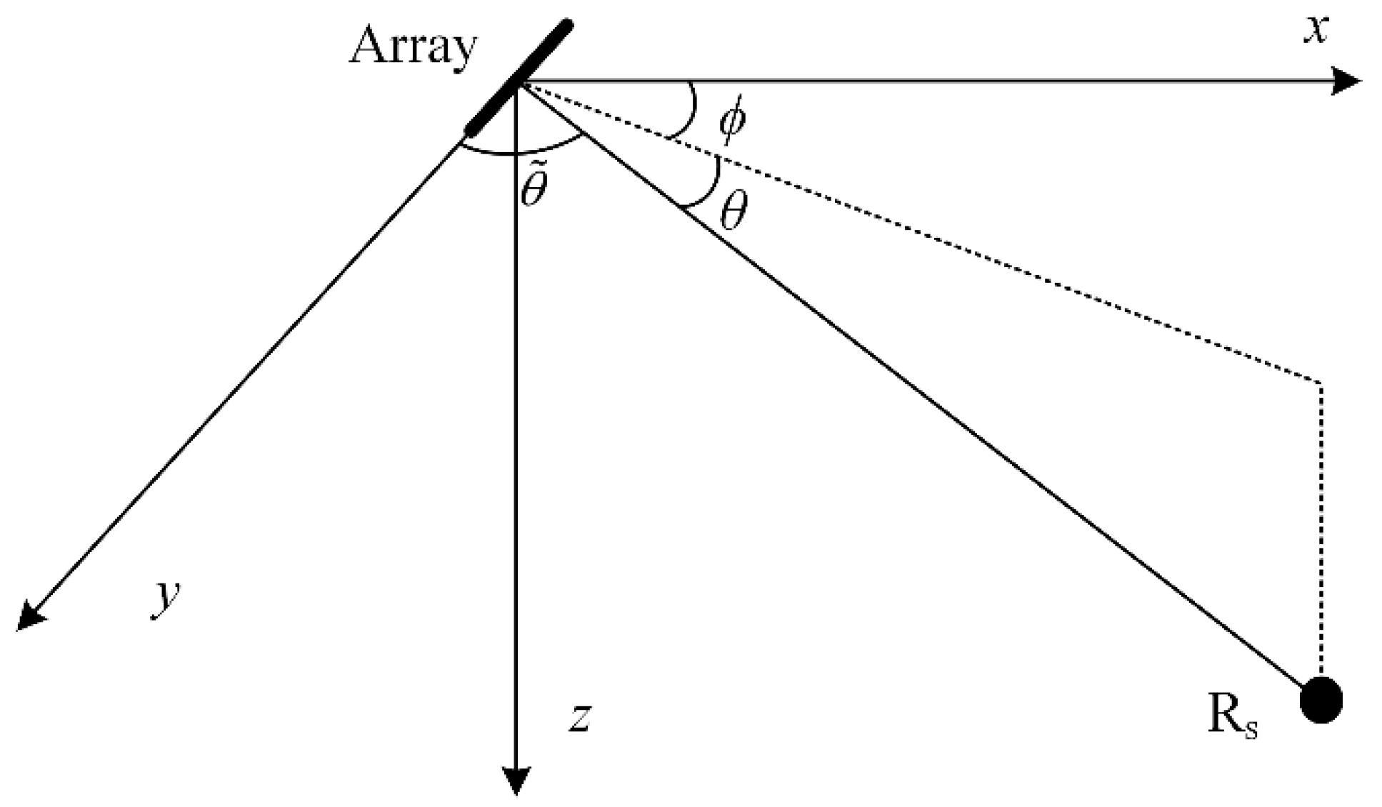
For the array-invariant method, extracting the Green’s function with blind deconvolution [8,9,11] from the received signals is necessary. Assume that an unknown source signal is . The frequency spectrum of is , where is the radian frequency and , is the corresponding phase. In this study, we focus on using a horizontal array in shallow water to realize passive localization. Consider a horizontal array with N elements, as shown in Figure 1. The received signal of the nth element can be expressed as
where and are the position vectors of the nth element of the array and the unknown source, respectively, and is the Green’s function between the source at and the nth element at . In a ray path approximation [11], the Green’s function can be written as
where is the horizontal azimuth shown in Figure 1, is the grazing angle of the kth ray, is the local time delay of the kth ray at the nth element, is travel times of the kth ray, and is the amplitude of the kth ray.
For the horizontal array in Figure 1, the local time delays depend mainly on the horizontal azimuth due to a small grazing angle, thus [11]. Subsequently, by steering the beam to , the output of the conventional plane-wave beamforming is identified by
Blind convolution uses the beamforming output phase, , and removes the phase component of the unknown source signal from by a phase rotation, expressed as:
The beam-time migration in the existing array-invariant method [11] can be obtained by processing the extracted with conventional plane-wave beamforming.
3. 2D Deconvolution for Obtaining Better Beam-Time Migration
To ensure our proposed method based on 2D deconvolution is easily understandable, frequency-domain conventional plane-wave beamforming is briefly introduced first in this section. Then, our proposed method is presented.
3.1. Conventional Plane-Wave Beamforming
Considering a far-field source, the angle of incidence is shown in Figure 1. When using uniform horizontal array, as shown in Section 2, with interelement spacing denoted by d, the received signal of the array can be expressed as
where is the array response vector given as , , and is the noise vector.
3.2. 2D Deconvolution
The local time delays in Equation (2) can be written as , which is the function of the beam angle measured , and can be abbreviated as . Then, the expression of the Green’s function in (2) can be rewritten as
Let . We define the 2D rotation matrix as
where , and .
Assuming that we process M samples, and are the start and end time of the sampling segment, respectively. Considering (7), after the time-beam rotation, the output can be written as
where and are the highest and lowest frequencies of the Green’s function in the discrete frequency domain, respectively. The power of is
After a simple derivation, Equation (10) can be written as a 2D convolution of the beam-time pattern, denoted as PSF, with the source power distribution . depends only on the difference in bearing and time, so is shift-invariant in the steering angle and time, and can be written as
where
and
It should be noted that separates the multiple arrivals, in terms of both the bearing and time domains, much better than does. If we estimate from using 2D deconvolution, high-resolution beam-time migration can be obtained, which helps improve the localization accuracy.
Some well-known deconvolution algorithms, such as the Richardson–Lucy (R–L) [12,13,14,15,16] algorithm, have been widely applied in various fields. We propose the use of the R–L algorithm to deconvolve both the bearing and time domains to improve the localization accuracy of the array-invariant method.
After obtaining the high-resolution beam-time migration, the range is estimated with the following formula:
where , which is extracted from the beam-time migration with the least-squares approach [2,11]. The source direction is estimated by searching for the maximum value in the beam-time migration.
4. Simulation
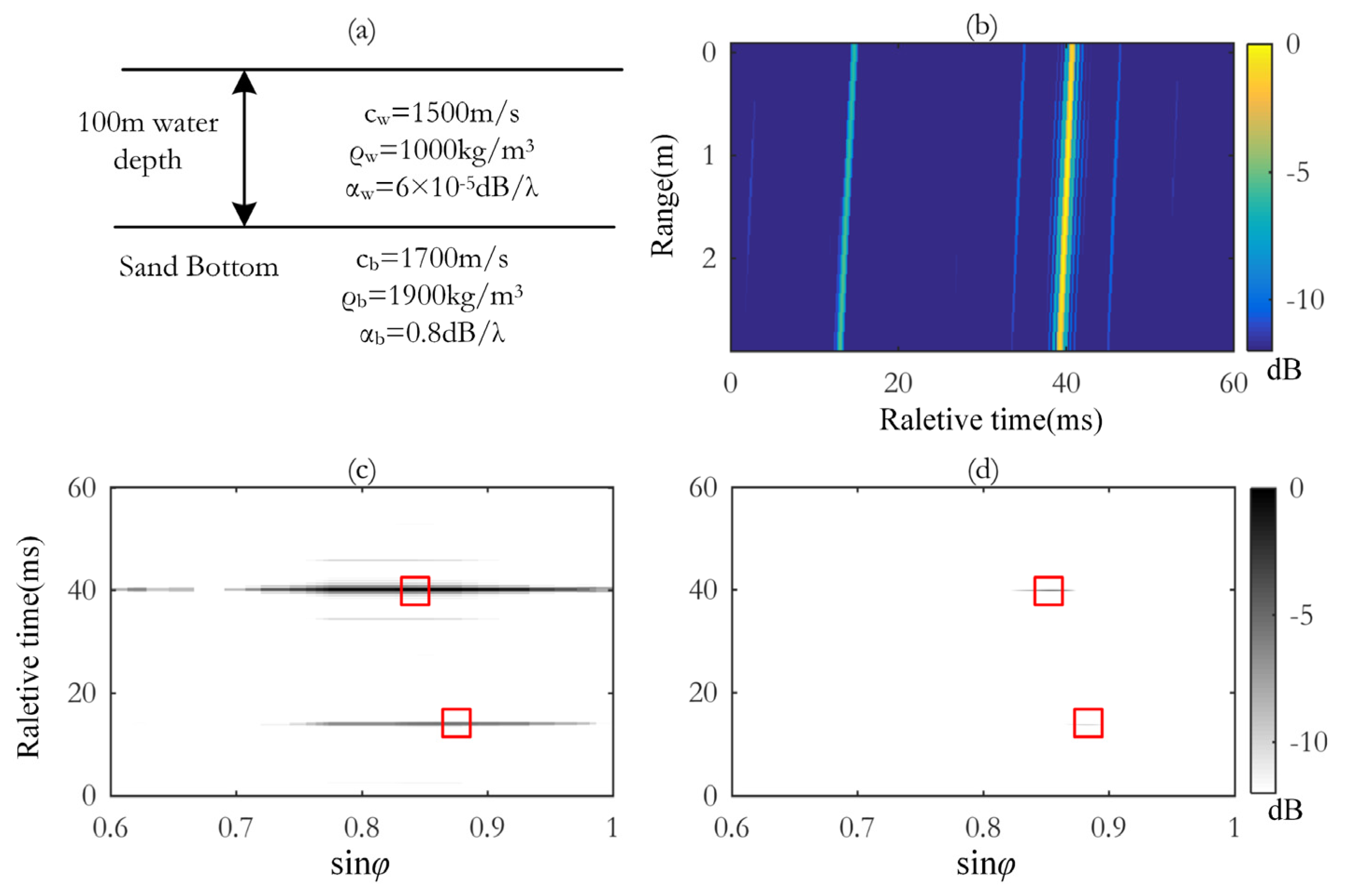
A simulation in a typical shallow-water waveguide was conducted to demonstrate our proposed method based on 2D deconvolution. The KRAKEN toolbox was used. The environmental parameters of the employed Pekeris [2,17] waveguide are summarized in Figure 2a. The water depth was 100 m and the speed of sound was assumed to be 1500 m and the same at different depths. The seabed was typically sand bottom.
A horizontal array with 16 elements was employed. The array length was 2.8 m. The bandwidth of the noise radiated by the source of opportunity was 2–4 kHz. The sampling frequency was 20 kHz. The existing array-invariant method [11] was used as the reference method. The source and the horizontal array were placed at 3 m and 97 m under water, respectively. The azimuth angle of the sound source was 65°. Additive white noise was used. The signal-to-noise ratio at each array element was set at 10 dB. The length of simulation data is 2 s. The Green’s function of the 16th element at the range of 1000 m was extracted with blind deconvolution and is shown in Figure 2b.
The beam-time migrations obtained using the reference method and proposed methods are shown in Figure 2c,d, respectively, which have the same scale. The peak position of beam-time migrations is marked by the red square. In Figure 2c, it can be seen that the relative arrival time of the two paths was 13.95 ms and 40.1 ms, respectively, and the sine of the beam angle of the two paths was 0.879 ms and 0.839 ms, respectively. In Figure 2d, it can be seen that the relative arrival time of the two paths was 13.2 ms and 40.1 ms, respectively, and the sine of the beam angle of the two paths was 0.883 ms and 0.849 ms, respectively.
It is clear that our proposed method based on 2D deconvolution, shown in Figure 2d, had a much higher resolution in both the bearing and time domains, compared to the reference method. Based on the high-resolution beam-time migration, it is clear that the source–range estimation error can be decreased.
For passive shallow-water localization with a horizontal array, the relative error of range estimation determines the localization accuracy. The source range was estimated according to Equation (14). In the case of the true source range of 1000 m, the range estimated with the reference method, shown in Figure 2c, was 850.2 m. The range estimated with the proposed method, shown in Figure 2d, was 1038.7 m. The relative estimation errors of the proposed and reference methods were 3.9% and 15.0%, respectively. The estimation performances of the two methods at different ranges are summarized in Table 1. On average, the estimation error of our proposed method was only one third of that of the reference method. The results also prove that the wideband beam-time migration obtained using conventional plane-wave beamforming in the reference array-invariant method [11] is one of the main factors influencing the accuracy of the source range estimation.
5. Experiment
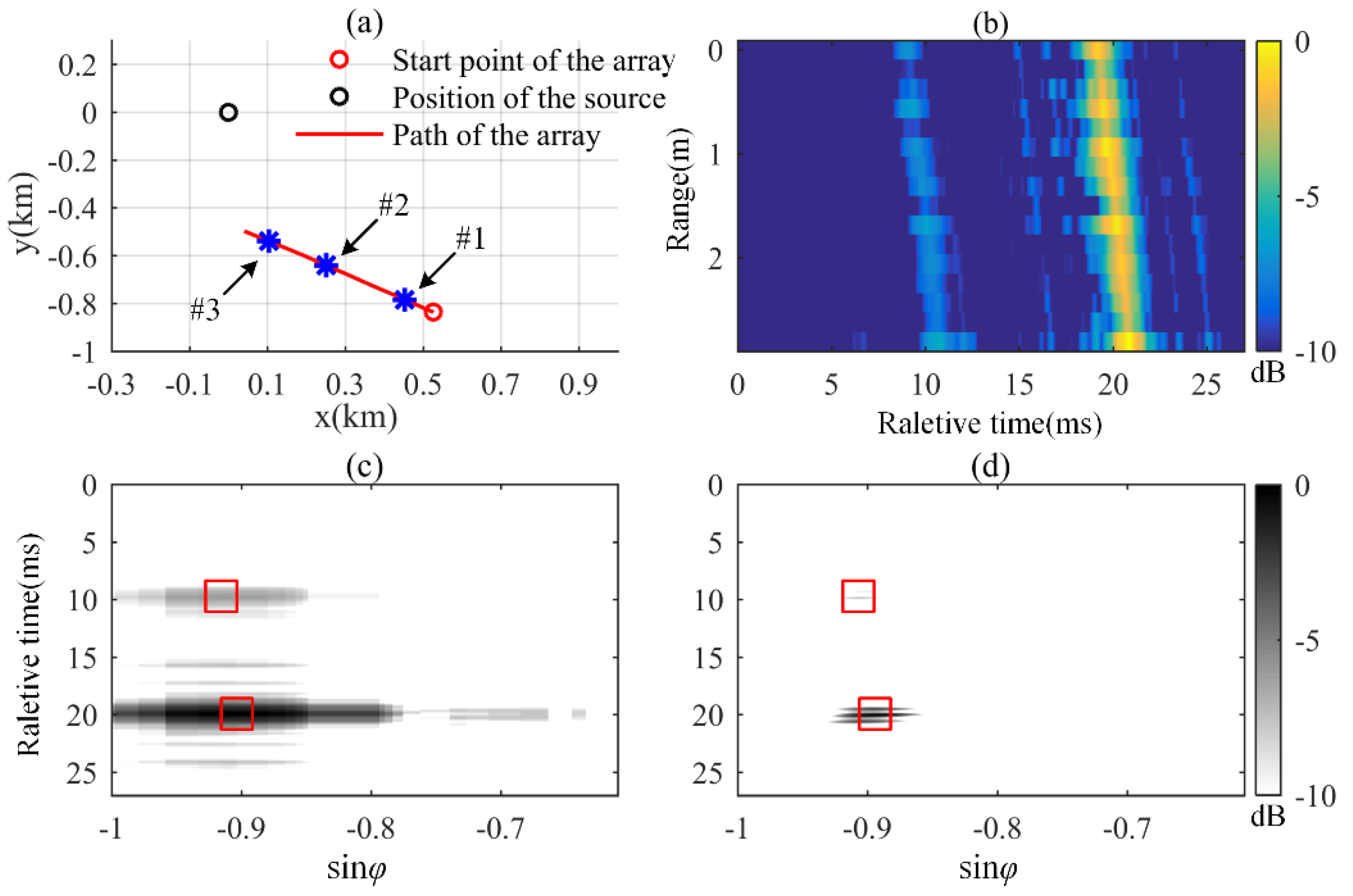
The data from an experiment in the Yellow Sea of China in 2019 were processed for testing the proposed and reference methods. A 2.8 m movable horizontal array was used. The horizontal array had 16 elements. The sampling frequency was 20 kHz. The source was fixed as shown in Figure 3a. The source transmitted wideband noise within a frequency band of 2–4 kHz. Both the source and the horizontal array were located at a depth of 5 m. The trajectory of the horizontal array is shown in Figure 3a.
The extracted Green’s function at Position #1 (988.9 m) in Figure 3a is shown in Figure 3b. The beam-time migrations obtained using the reference and proposed methods are shown in Figure 3c,d, respectively, which have the same scale. The peak position of beam-time migrations is marked by the red square. Based on the beam-time migrations in Figure 3c,d, the range estimated with the reference and proposed methods were 1244.3 m and 1130.2 m, respectively, and the relative estimation errors of the reference and proposed methods were 25.9% and 14.4%, respectively.
The received signals at Positions #2 (718.6) and #3 (580.1) in Figure 3a were also processed with the proposed and reference methods. Table 2 shows the range estimates and relative errors of the proposed and reference methods at different positions. It can be seen that the relative error of the proposed method is about half of that of the reference method.
6. Conclusions
This brief report proposed an array-invariant method based on 2D deconvolution for robust passive source localization in shallow water. Our proposed method achieved much better beam-time migration than the existing array-invariant method, which improved the range estimation accuracy significantly. Both the simulation and the experiment show that our proposed method based on 2D deconvolution achieves a much higher accuracy than the existing array-invariant method. This brief report also reveals that the relatively wideband beam-time migration obtained using conventional plane-wave beamforming in the existing array-invariant method is one of the main factors that influences the localization accuracy.
Author Contributions
Conceptualization, Y.W. and C.C.; methodology, Y.W. and C.C.; software, Y.W.; validation, Y.W.; data curation, Y.W.; writing—original draft preparation, Y.W., C.C. and D.J.; writing—review and editing, Y.L. and H.H. All authors have read and agreed to the published version of the manuscript.
Funding
This research was supported by the National Natural Science Foundation of China under grant 62201565 and grant 62001469.
Institutional Review Board Statement
The study did not require ethical approval.
Informed Consent Statement
The study did not involve humans in this paper.
Data Availability Statement
The study did not report any data.
Conflicts of Interest
The authors declare no conflict of interest.
References
- Hotkani, M.M.; Bousquet, J.-F.; Seyedin, S.A.; Martin, B.; Malekshahi, E. Underwater Target Localization Using Opportunistic Ship Noise Recorded on a Compact Hydrophone Array. Acoustics 2021, 3, 611–629. [Google Scholar] [CrossRef]
- Lee, S.; Makris, N.C. The array invariant. J. Acoust. Soc. Am. 2006, 119, 336–351. [Google Scholar] [CrossRef] [PubMed]
- Sabra, K.G.; Song, H.-C.; Dowling, D.R. Ray-based blind deconvolution in ocean sound channels. J. Acoust. Soc. Am. 2010, 127, EL42–EL47. [Google Scholar] [CrossRef] [PubMed]
- Byun, S.; Verlinden, C.; Sabra, K. Blind deconvolution of shipping sources in an acoustic waveguide. J. Acoust. Soc. Am. 2017, 141, 797–807. [Google Scholar] [CrossRef] [PubMed]
- Byun, S.-H.; Byun, G.; Sabra, K.G. Ray-based blind deconvolution of shipping sources using multiple beams separated by alternating projection. J. Acoust. Soc. Am. 2018, 144, 3525–3532. [Google Scholar] [CrossRef] [PubMed]
- Cho, C.; Song, H.C.; Hodgkiss, W.S. Robust source-range estimation using the array/waveguide invariant and a vertical array. J. Acoust. Soc. Am. 2016, 139, 63–69. [Google Scholar] [CrossRef] [PubMed]
- Song, H.C.; Cho, C. Array invariant-based source localization in shallow water using a sparse vertical array. J. Acoust. Soc. Am. 2017, 141, 183–188. [Google Scholar] [CrossRef] [PubMed]
- Byun, G.; Kim, J.S.; Cho, C.; Song, H.C.; Byun, S.-H. Array invariant-based ranging of a source of opportunity. J. Acoust. Soc. Am. 2017, 142, EL286–EL291. [Google Scholar] [CrossRef] [PubMed]
- Byun, G.; Song, H.C.; Byun, S.-H. Localization of multiple ships using a vertical array in shallow water. J. Acoust. Soc. Am. 2019, 145, EL528–EL533. [Google Scholar] [CrossRef] [PubMed]
- Gong, Z.; Ratilal, P.; Makris, N.C. Simultaneous localization of mul-tiple broadband non-impulsive acoustic sources in an ocean waveguide using the array invariant. J. Acoust. Soc. Am. 2015, 138, 2649–2667. [Google Scholar] [CrossRef] [PubMed] [Green Version]
- Byun, G.; Song, H.C.; Kim, J.S.; Park, J.S. Real-time tracking of a surface ship using a bottom-mounted horizontal array. J. Acoust. Soc. Am. 2018, 144, 2375–2382. [Google Scholar] [CrossRef] [PubMed]
- Yang, T.C. Deconvolved Conventional Beamforming for a Horizontal Line Array. IEEE J. Ocean. Eng. 2017, 43, 160–172. [Google Scholar] [CrossRef]
- Chi, C.; Li, Z.; Li, Q. Fast Broadband Beamforming Using Nonuniform Fast Fourier Transform for Underwater Real-Time 3-D Acoustical Imaging. IEEE J. Ocean. Eng. 2015, 41, 249–261. [Google Scholar] [CrossRef]
- Chi, C.; Li, Z.; Li, Q. Ultrawideband Underwater Real-Time 3-D Acoustical Imaging with Ultrasparse Arrays. IEEE J. Ocean. Eng. 2016, 42, 1–12. [Google Scholar] [CrossRef]
- Chi, C. Underwater Real-Time 3D Acoustical Imaging: Theory, Algorithm and System Design; Springer: Berlin/Heidelberg, Germany, 2019; Chapter 4. [Google Scholar]
- Blahut, R.E. Theory of Remote Image Formation; Cambridge University Press: Cambridge, MA, USA, 2004; Chapters 9 and 11. [Google Scholar]
- Jensen, F.B.; Kuperman, W.A.; Porter, M.B.; Schmidt, H. Computational Ocean Acoustics; Springer: New York, NY, USA, 2011; Chapters 3 and 5. [Google Scholar]
Figure 1.
Coordinate system defined with the azimuth angle , beam angle , and the grazing angle of incoming ray arrival [10].
Figure 1.
Coordinate system defined with the azimuth angle , beam angle , and the grazing angle of incoming ray arrival [10].

Figure 2.
(a) The Pekeris waveguide with sand bottom, where , , and are the sound speed, density of the water, and attenuation of the water, and , and correspond to those in the sand. (b) The Green’s function was obtained with blind deconvolution at a distance of 1000 m between the array and source. (c) Beam-time migration obtained using the reference method. (d) Beam-time migration obtained using the proposed method.

Figure 3.
(Color online). (a) Positions of the array and source in the experiment. (b) Green’s function obtained with blind deconvolution at Position #1. (c) Beam-time migration obtained using the reference method. (d) Beam-time migration obtained using the proposed method.
Figure 3.
(Color online). (a) Positions of the array and source in the experiment. (b) Green’s function obtained with blind deconvolution at Position #1. (c) Beam-time migration obtained using the reference method. (d) Beam-time migration obtained using the proposed method.


Table 1.
The range estimates and relative errors of the proposed and reference methods at different ranges in the simulation.
Table 1.
The range estimates and relative errors of the proposed and reference methods at different ranges in the simulation.
| True Range | Proposed (Estimated Range, Relative Error) | Reference (Estimated Range, Relative Error) |
|---|---|---|
| 1000 m | 1038.7 m, 3.9% | 850.2 m, 15.0% |
| 1500 m | 1615.1 m, 7.7% | 1216.3 m, 18.9% |
| 2000 m | 2146.8 m, 7.3% | 2454.3 m, 22.7% |
| 3000 m | 3232.3 m, 7.7% | 2251.0 m, 24.9% |
Table 2.
The range estimates and relative errors of the proposed and reference methods at different ranges in the experiment.
Table 2.
The range estimates and relative errors of the proposed and reference methods at different ranges in the experiment.
| True Range | Proposed (Estimated Range, Relative Error) | Reference (Estimated Range, Relative Error) |
|---|---|---|
| #1 (988.9 m) | 1130.2 m, 14.4% | 1244.3 m, 25.9% |
| #2 (718.6 m) | 604.2 m, 15.9% | 535.3 m, 25.3% |
| #3 (580.1 m) | 515.2 m, 11.2% | 425.5 m, 26.6% |
Publisher’s Note: MDPI stays neutral with regard to jurisdictional claims in published maps and institutional affiliations. |
© 2022 by the authors. Licensee MDPI, Basel, Switzerland. This article is an open access article distributed under the terms and conditions of the Creative Commons Attribution (CC BY) license (https://creativecommons.org/licenses/by/4.0/).
Share and Cite
MDPI and ACS Style
Wang, Y.; Chi, C.; Li, Y.; Ju, D.; Huang, H. Passive Array-Invariant-Based Localization for a Small Horizontal Array Using Two-Dimensional Deconvolution. Appl. Sci. 2022, 12, 9356. https://doi.org/10.3390/app12189356
AMA Style
Wang Y, Chi C, Li Y, Ju D, Huang H. Passive Array-Invariant-Based Localization for a Small Horizontal Array Using Two-Dimensional Deconvolution. Applied Sciences. 2022; 12(18):9356. https://doi.org/10.3390/app12189356
Chicago/Turabian StyleWang, Yujie, Cheng Chi, Yu Li, Donghao Ju, and Haining Huang. 2022. "Passive Array-Invariant-Based Localization for a Small Horizontal Array Using Two-Dimensional Deconvolution" Applied Sciences 12, no. 18: 9356. https://doi.org/10.3390/app12189356
Note that from the first issue of 2016, this journal uses article numbers instead of page numbers. See further details here.