

Semi-Direct Point-Line Visual Inertial Odometry for MAVs
School of Electronics and Information, Northwestern Polytechnical University, Xi’an 710072, China
*
Author to whom correspondence should be addressed.
Appl. Sci. 2022, 12(18), 9265; https://doi.org/10.3390/app12189265
Submission received: 22 August 2022
/
Revised: 8 September 2022
/
Accepted: 13 September 2022
/
Published: 15 September 2022
(This article belongs to the Topic Multi-Sensor Integrated Navigation Systems)
Abstract
:Traditional Micro-Aerial Vehicles (MAVs) are usually equipped with a low-cost Inertial Measurement Unit (IMU) and monocular cameras, how to achieve high precision and high reliability navigation under the framework of low computational complexity is the main problem for MAVs. To this end, a novel semi-direct point-line visual inertial odometry (SDPL-VIO) has been proposed for MAVs. In the front-end, point and line features are introduced to enhance image constraints and increase environmental adaptability. At the same time, the semi-direct method combined with IMU pre-integration is used to complete motion estimation. This hybrid strategy combines the accuracy and loop closure detection performance of the feature-based method with the rapidity of the direct method, and tracks keyframes and non-keyframes, respectively. In the back-end, the sliding window mechanism is adopted to limit the computation, while the improved marginalization method is used to decompose the high-dimensional matrix corresponding to the cost function to reduce the computational complexity in the optimization process. The comparison results in the EuRoC datasets demonstrate that SDPL-VIO performs better than the other state-of-the-art visual inertial odometry (VIO) methods, especially in terms of accuracy and real-time performance.
1. Introduction
A navigation system is one of the main applications for MAVs [1], mainly providing accurate and reliable attitude, speed and position information, and is indispensable in the process of MAVs flight and control. Due to limitations in size and payload capacity, MAVs are typically equipped with low-cost sensors and lack the hardware required to run advanced integrated navigation algorithms. Designing a low-cost integrated navigation platform for MAVs and building a more efficient system on this basis to ensure accuracy and real-time performance is the basic premise for MAVs to perform tasks and even survive.
Visual Inertial Navigation (VIN) is a hot topic in the field of MAVs research [2,3]. Cameras can provide abundant visual information, and inertial sensors (gyroscopes and accelerometers) can provide short-term and high-precision pose estimation. Their low cost, low power, small size, and complementarity make a combination of them particularly suitable for MAVs.
Based on the functional structure, VINs can be classified into the front end and the back end. The front end completes the calculation of visual and inertial motion states, and the back end realizes data fusion and outputs the optimal state estimation.
Front-end image processing methods can be divided into the following: (1) Feature-based methods [4,5,6,7,8,9,10,11,12], which extract representative features (such as point or line features) from images, and then match them according to the description of features. OKVIS [5] finds features using the Harris corner detector, and matches them using Binary robust invariant scalable keypoints (BRISK) descriptors. ORB-SLAM2 [7] performs feature extraction, description and matching, and then performs motion estimation using Oriented FAST and Rotated BRIEF (ORB) features. PL-SLAM [8] integrates the line representation within the SLAM, and improves the performance of ORB-SLAM2, especially in poorly textured environments. However, feature extraction and the calculation of descriptors are very time-consuming. (2) Direct methods [13,14], which estimate the motion based on the pixel gray difference between two images. DSO [14] minimizes the photometric error to estimate the camera motion, which greatly reduces the amount of computation compared with feature-based methods. However, it has high requirements regarding image quality and is not suitable for large inter-frame motion. (3) Semi-direct methods [15,16,17,18,19,20,21,22], which combine the above two methods and have received increasing attention from researchers in recent years. SVO [15] first uses the image intensity to estimate the pose, and then uses the position of feature points to optimize the pose. However, there are still shortcomings in motion-tracking accuracy and robustness. PL-SVO [16] extends line segments to the SVO algorithm, and has stronger robustness in poorly textured environments. SVL [18] combines ORB-SLAM and SVO, in which the former is used in keyframes and the latter is used in non-keyframes. PCSD-VIO [22] refers to the frame-tracking strategy of SVL, but integrates online photometric calibration, and the fusion method with IMU is slightly different.
Back-end data fusion methods can be divided into the following: (1) Filtering-based methods [4,6], which use inertial observation for state propagation and visual observation for state update. As the number of features in the state vector increases, the computational complexity rapidly increases, so it is not suitable for a large range of scenes. (2) Optimization-based methods [5,9,10,11,23,24,25,26,27,28], which are usually based on keyframes and minimize the overall errors by establishing the connection relation between frames and constantly adjusting the pose of frames. VINS-Mono [10] is a tightly coupled algorithm based on nonlinear optimization, with initialization, loop detection and relocalization modules. PL-VIO [11] adds line features to the basic frame of VINS-Mono, and has achieved good results. However, it lacks a loop-detection module, and uses a large amount of computation in nonlinear optimization.
The above work has both advantages and disadvantages, such as the adoption of time-consuming feature extraction, sensitivity to poorly textured environments and large illumination changes, ability to work without inertial sensors, and the large amount of computation needed in nonlinear optimization. Therefore, a novel, semi-direct, point-line, visual inertial odometry for MAVs has been proposed. The main contributions are as follows:
Firstly, motion estimation is accomplished using the semi-direct method, which realizes the mutual advantage compensation of the feature-based method and the direct method, that is, the former accurately tracks keyframes, and extracts point and line features for back-end nonlinear optimization and loop-closure detection, while the latter rapidly tracks non-keyframes through direct image alignment.
Secondly, the sliding window mechanism is adopted to effectively combine visual and inertial information, and an improved marginalization method is used to decompose the high-dimension matrix corresponding to the cost function, which binds the computational complexity and improves the computational efficiency.
Finally, experiments are conducted to compare SDPL-VIO and the other state-of-the-art VIO methods. The results of the European Robotics Challenge (EuRoC) datasets show that SDPL-VIO can consider both speed and accuracy.
2. Mathematical Formulation
2.1. Notations
We define {w}, {b}, {c} as a world coordinate, body coordinate and camera coordinate, respectively. and are the rotation and translation from the world coordinate to the camera coordinate. and represent the extrinsic parameters, which can be calibrated in advance. is the 4 × 4 homogeneous transformation. is the quaternion representation of , ⊗ represents the multiplication between two quaternions. represents the skew symmetric matrix corresponding to the vector.
2.2. IMU Pre-Integration
The raw IMU measurements (angular velocity and acceleration ) are affected by gravity , bias and noise [10]:
where, and are the real IMU measurements.
The IMU state propagation from the consecutive frame to can be given by:
where,
where , and are the pre-integrated measurements, and .
2.3. Point Feature Projection
For a pin-hole camera model, the projection from the camera coordinate to the camera image plane can be defined as:
where represent camera intrinsic parameters.
2.4. Line Feature Projection
The Plücker coordinates [29] is used for line parameterization. A 3D line representing the Plücker coordinates is constructed as , where represents the normal vector of the plane determined by the line and the coordinate origin, and represents the line direction vector. According to the description in [30], the transformation of a 3D line from the world coordinate to the camera coordinate can be defined as:
and the projection from the camera coordinate to the camera image plane can be defined as:
where represents the projection matrix of line .
3. Proposed System Implementation
3.1. System Framework
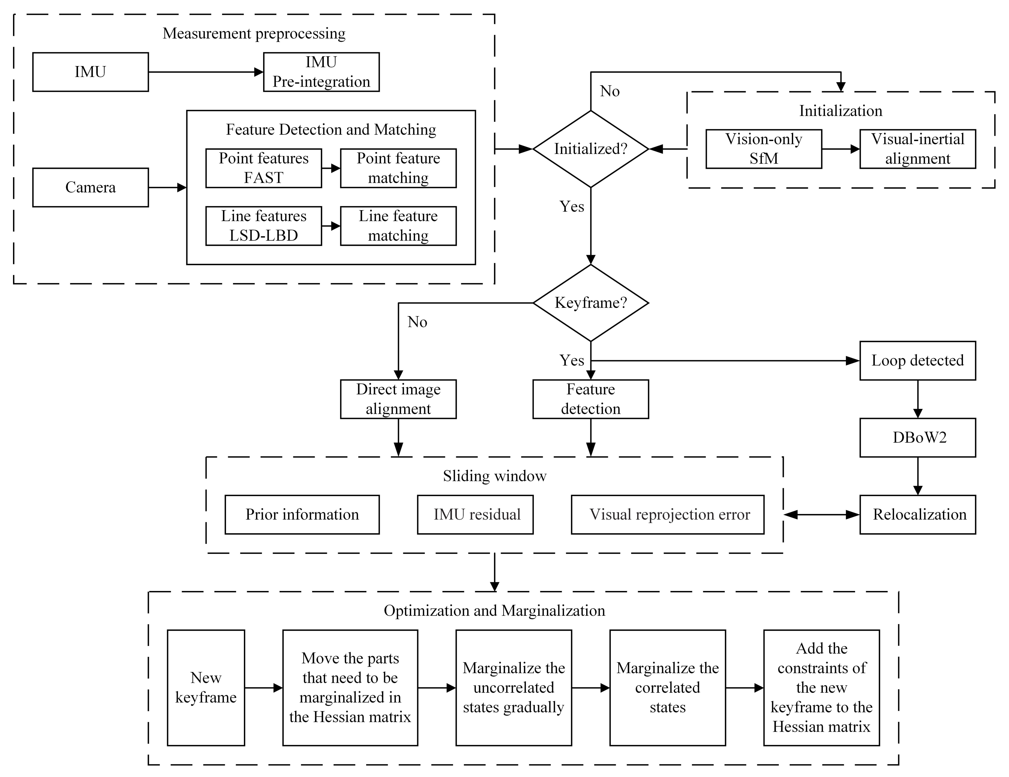
The proposed system mainly includes two parts: front-end image tracking (measurements preprocessing and initialization), back-end nonlinear optimization, marginalization and loop closure detection, as shown in Figure 1. In the front end, the system extracts point and line features from the image, and carries out a motion estimation of adjacent image frames combined with IMU pre-integration. By aligning visual and inertial information, visual inertial joint initialization is performed to restore metric scale, and estimate inertial bias and gravity vector. Then, after judging whether the current frame is a keyframe according to the selection criteria, the system uses the semi-direct method to track keyframes and non-keyframes, respectively. In the back end, the system adopts a cost function to obtain the optimal state estimation by minimizing prior information, IMU residuals and visual re-projection errors, and uses improved marginalization to decompose the high-dimension matrix step-by-step, corresponding to the cost function, which optimizes the solution and improves the computational efficiency. The key processes are described in detail in the following sections.
3.2. Front-End Tracking Based on Semi-Direct Methods
3.2.1. Visual-Inertial Initializaiton
We conducted measurement preprocessing, and completed the visual-inertial initialization by aligning the results of vision-only Structure from Motion (SFM) and IMU pre-integration. The system first performed this process to restore the metric scale and estimate the inertial bias and the gravity vector. The specific initialization process can be referred to in [11].
3.2.2. Keyframe Selection
After initialization, the system determines whether the current frame is a keyframe based on scene changes and IMU pre-integration. The overall output accuracy of the system depends largely on the quality of the keyframes that were inserted. The selection criteria for keyframes are as follows: First, the average parallax of tracked points between the current frame and the latest keyframe is beyond a certain threshold. Second, the number of tracked points goes below a certain threshold. Third, the translation calculated by IMU pre-integration exceeds a preset threshold after the latest keyframe is inserted. If any of the above criteria are met, the current frame is considered a keyframe.
3.2.3. Semi-Direct Method for Tracking
(a) For keyframes, we detected point features using the Accelerated Segment Test (FAST) [31] algorithm and tracked adjacent frames using an optical flow based on Kanade-Lucas-Tomasi (KLT) [32]. Then, we eliminated outliers by Random Sample Consensus (RANSAC) combined with the essential matrix model. Meanwhile we detected line segments using the Line Segment Detector (LSD) [33] algorithm, and matched them using Line Band Descriptors (LBD) [34] between the current frame and the reference frame. In addition, we also removed outliers for line-matching using geometric constraints.
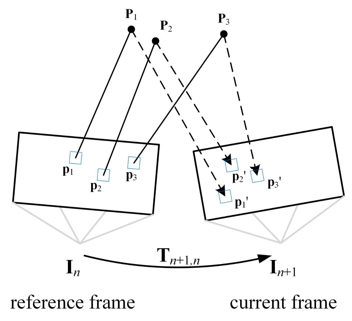
(b) For non-keyframes, as shown in Figure 2, we first extracted the key points from the last keyframe in the sliding window, and used transformation to construct the matching 3D points in the world coordinate. Then, we projected the 3D points onto the current frame , and obtained the pixel intensity residual as:
where is the image area formed by the key points . By minimizing the photometric error, the relative pose can be calculated [15]:
where .
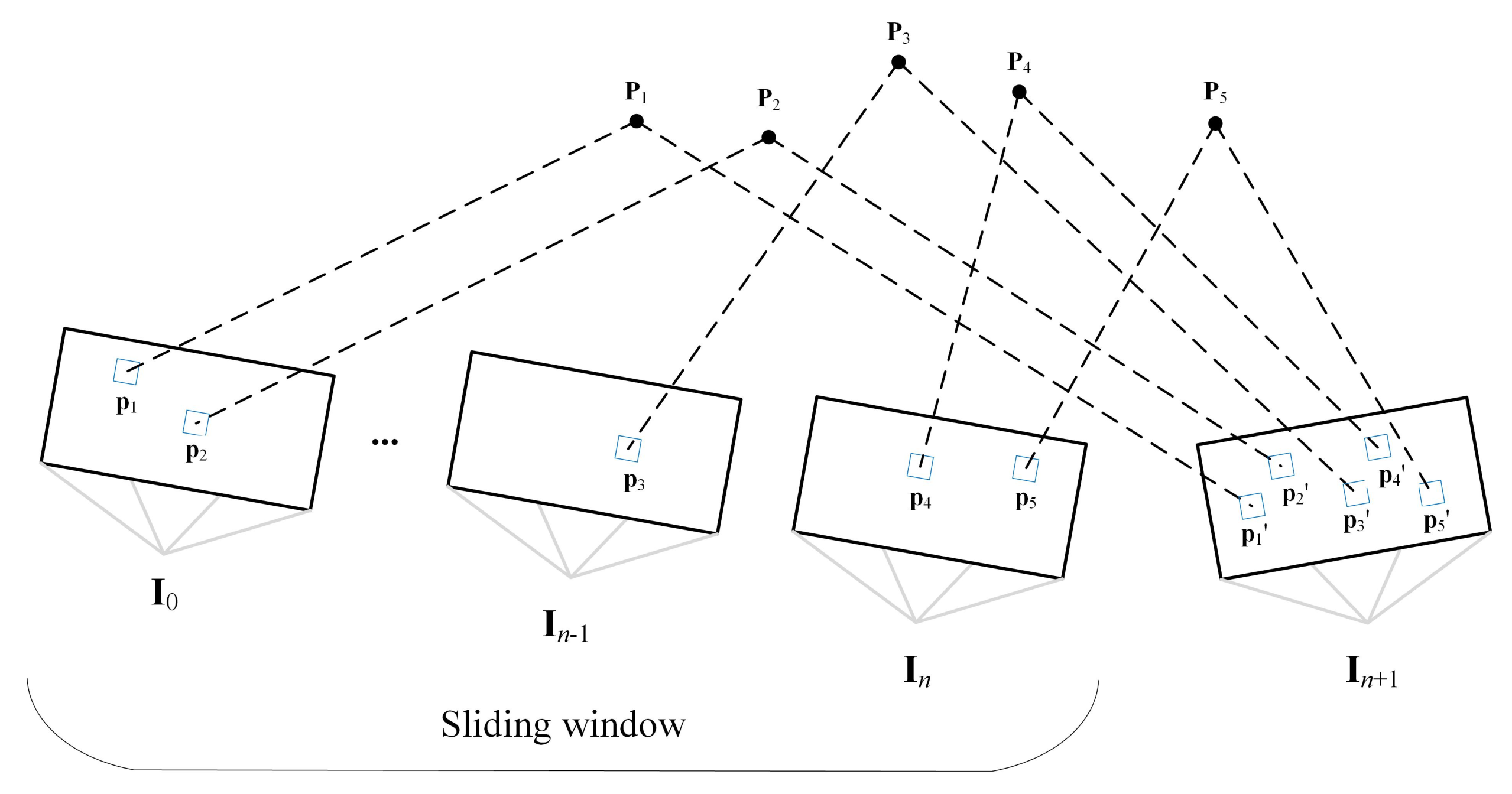
However, the current frame pose, which was only obtained by Equation (8), is insufficiently accurate. Therefore, we need to find more co-visibility feature points between the current frame and the co-visibility keyframes in the sliding window. As shown in Figure 3, based on the pose solved by Equation (8), we projected the co-visible 3D points in the world coordinate onto the current frame. By minimizing the photometric error of co-visibility points, the corresponding 2D feature points in the current frame can be obtained:
After feature-points-matching was completed, we again optimized the camera pose to minimize the re-projection errors:
3.3. Back-End Optimization
3.3.1. Sliding Window Formulation
The sliding window [28] limits the number of keyframes and prevents the number of poses and features from increasing over time, so that back-end optimization is always within a limited complexity. The full state variables in the sliding window are defined as:
where is the ith IMU state. , , and represent position, velocity and orientation, respectively. and represent acceleration bias and gyroscope bias, respectively. represent the point landmarks, and are the 3D line representation formed by the Plücker coordinates. m and o are the number of point and line features in the sliding window, respectively.
The cost function, which simultaneously optimizes visual and IMU variables, is shown in Equation (12):
where are the prior information from marginalization, are the IMU measurement residuals, is the set of IMU states. and are the point and line feature re-projection errors, respectively. and are the set of observed point and line features, and is the Cauchy loss function, which minimizes the influence of outliers. Therefore, the matching error terms can be expressed as follows:
- (a)
- IMU measurement residual
According to Equations (1)–(3), the IMU measurement residuals for two consecutive frames can be calculated as follows:
where extracts the vector part of the quaternion.
- (b)
- Point feature error term
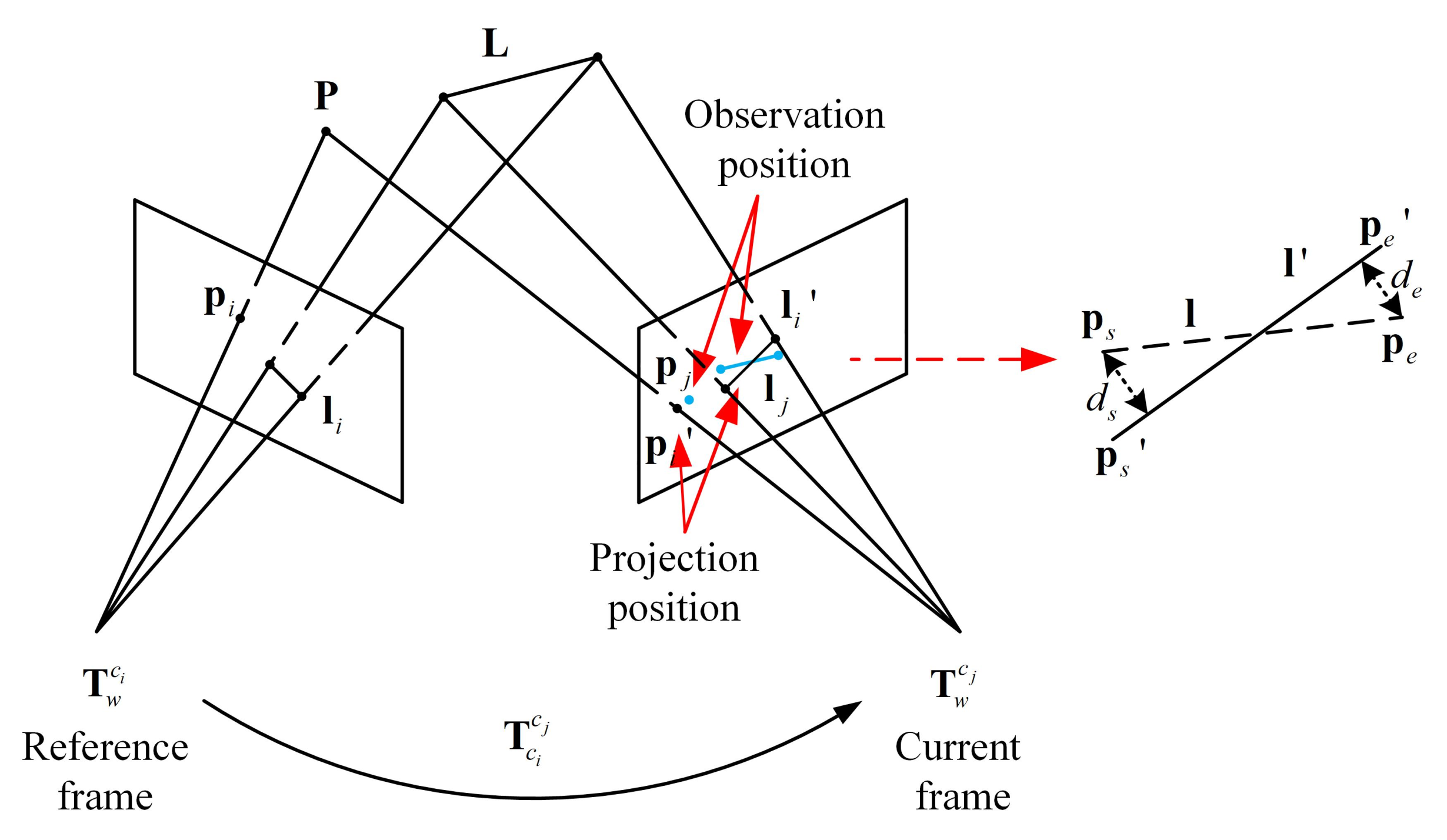
As shown in Figure 4, the point feature re-projection error is represented as the distance between the observed projection position and currently estimated projection position of the 3D point, which can be defined as:
where is the observed point in camera frame j and is the matching 3D point.
The Jacobian of the point feature re-projection error relative to the pose increment can be obtained by the chain rule:
with
- (c)
- Line feature error term
According to Figure 4, the line feature re-projection error is represented as the distance from two endpoints ( and ) of the matching line segment to the projecting line . Combining Equations (5) and (6), this can be calculated as below [29]:
where,
The Jacobian line feature re-projection error relative to the pose increment can be obtained as follows:
with
3.3.2. Improved Marginalization
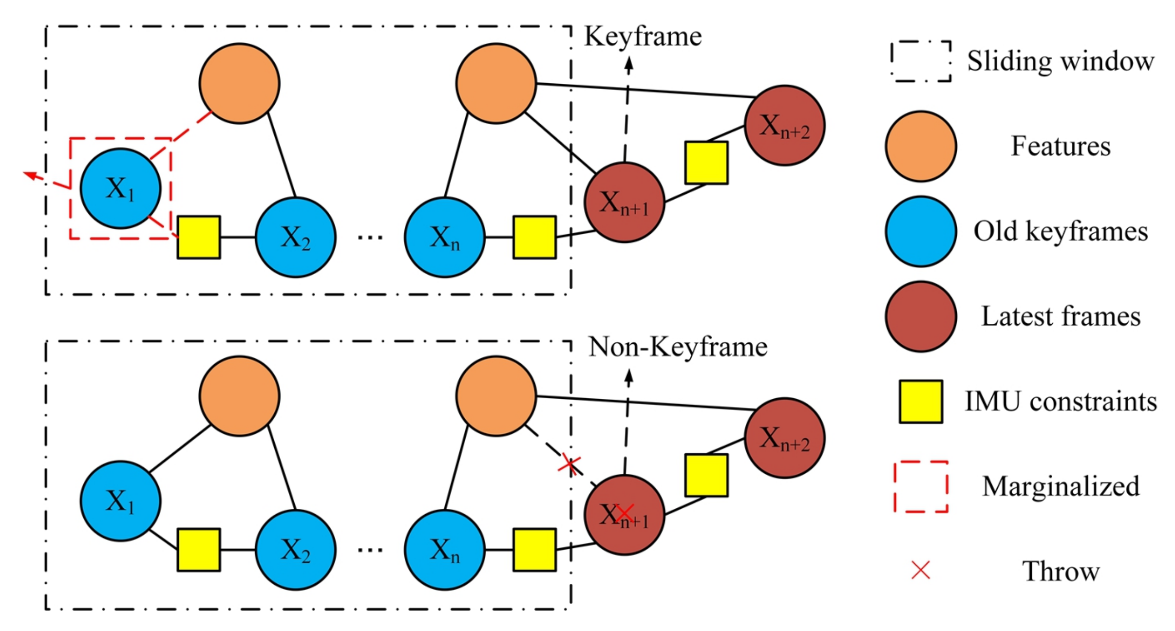
Marginalization is performed to bound the computational complexity, and the illustration is shown in Figure 5. If the second latest frame is a keyframe, the system will marginalize the oldest frame, including the pose of the oldest frame and some observed visual landmarks. When the oldest frame has co-visibility with other keyframes in the sliding window, that is, they observe the same visual landmarks, marginalization will keep the constraint on other keyframes. Otherwise, the system will retain the IMU measurements attached to this non-keyframe but remove the visual measurements.
This process is solved by the Gauss–Newton iterative method and defined in the form :
where represents the set of states that are to be marginalized and represents the set of preserved states [23,24].
Through the Schur complement, can be obtained:
which describes the basic marginalization. Thus, the states in are marginalized together. Equation (25) requires calculating , in which the computational complexity is , supposing that and have dimensions of and .
The above basic marginalization method has high computational complexity, so we adopted the improved marginalization method to solve this problem. Firstly, we divided the state vector which was be marginalized into two parts: one was uncorrelated states, containing visual landmarks, the other was correlated states, containing the pose of keyframes, velocity and IMU bias. Uncorrelated states were not related to each other, only to correlated states [24].
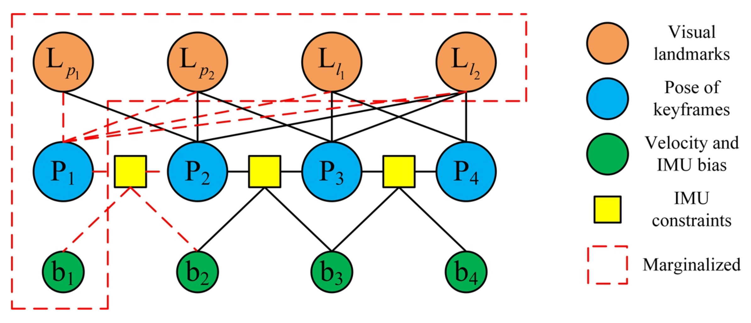
We described this process using an example, as shown in Figure 6. The states that are to be marginalized are represented by dashed lines, where and are points and line segments, respectively, are the pose of keyframes, and are velocity and IMU bias.
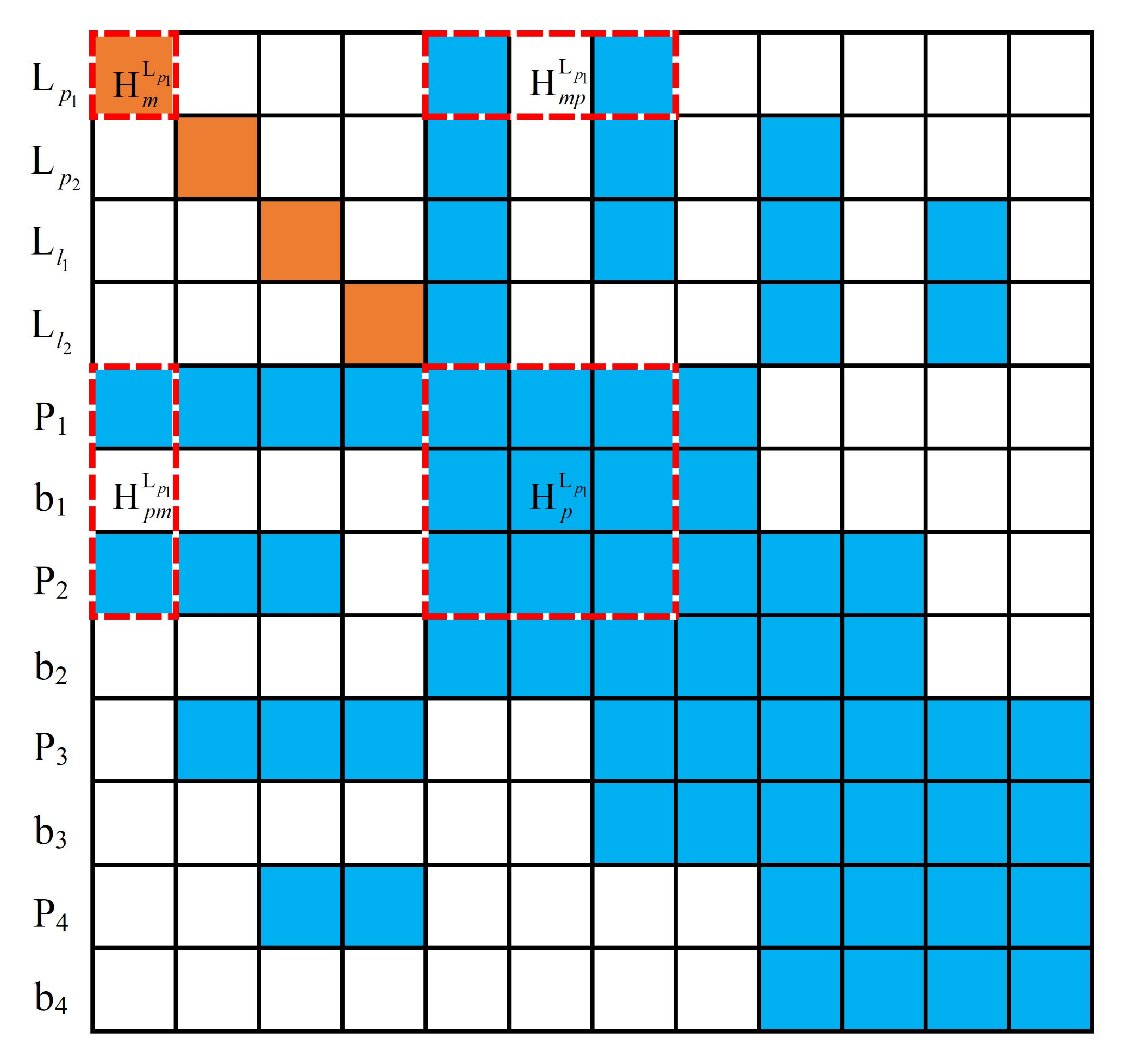
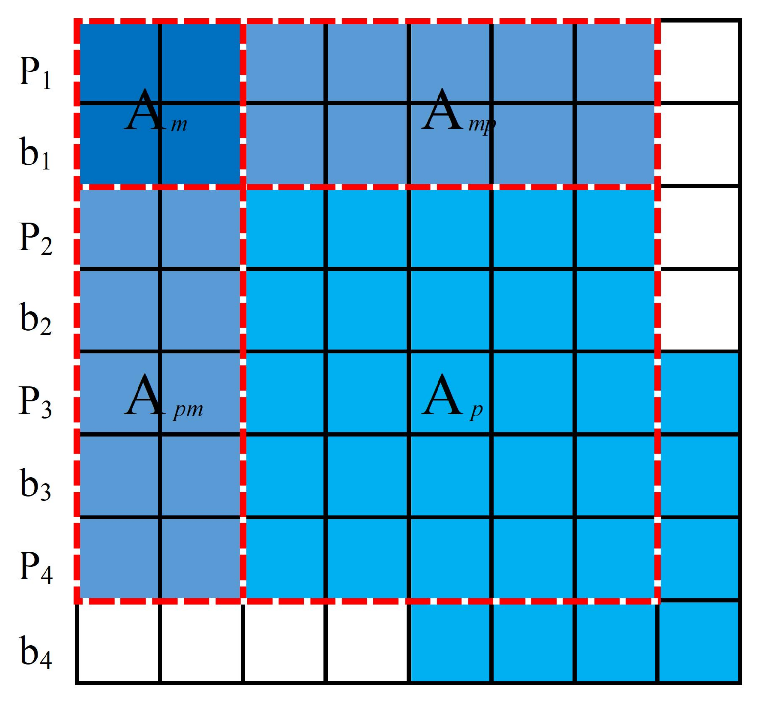
Figure 7 shows the corresponding Hessian matrix. The state variable that is to be marginalized is , while the state variable that is to be preserved is .
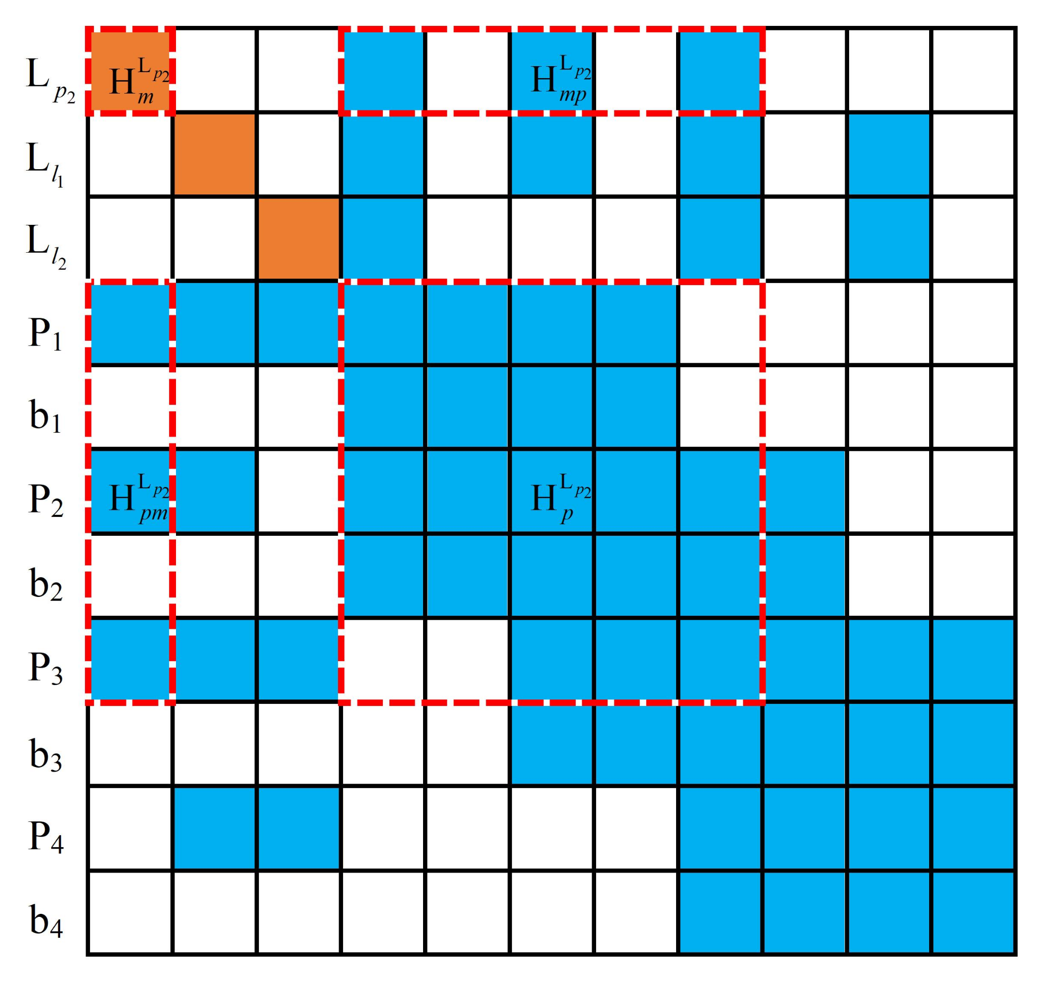
Firstly, uncorrelated states in were marginalized, which only contain points and line segments (, , and ). The computational complexity for the marginalization of in Figure 7 was mainly determined by , which is approximately . The maximum computational complexity will be , supposing that can be observed by , and . The Hessian matrix after the marginalization of is shown in Figure 8.
will be marginalized after the marginalization of , which requires calculating , and the computational complexity is approximately .
The remaining and were marginalized in the same way, with a computational complexity of . The Hessian matrix after the marginalization of uncorrelated states is shown in Figure 9. Then, correlated states that contain and in were marginalized, by calculating , with a computational complexity of . Therefore, the total computational complexity will be .
Through the above analysis, it is obvious that, compared with the basic marginalization method corresponding to Equation (25), the improved marginalization method greatly reduces the amount of computation.
3.3.3. Loop Closure Detection
For loop closure detection, we adopted Bags of Words (DBoW2) [35], a state-of-the-art bag-of words place recognition approach. The loop closure detection module will be activated when the current frame is selected as a keyframe. If a loop closure is detected, the drift accumulated during the exploration will be greatly reduced [10].
4. Experimental Results and Analysis
We compared SDPL-VIO with the state-of-the-art methods: SVO [17], PCSD-VIO [22], PL-VIO [11] and VINS-Mono [10] on the EuRoC datasets [36]. The EuRoC datasets were collected by various sensors installed on the MAV, and divided into three series of flight scenarios, including a series of motion sequences ranging from easy to difficult. First, the comparison results of the accuracy and robustness performance based on the datasets are shown in Section 4.1. Then, to demonstrate the computation performance of SDPL-VIO, the time usage statistics results are illustrated in Section 4.2. Finally, the loop-closure detection capability of SDPL-VIO is evaluated in Section 4.3.
4.1. Accuracy and Robustness Performance
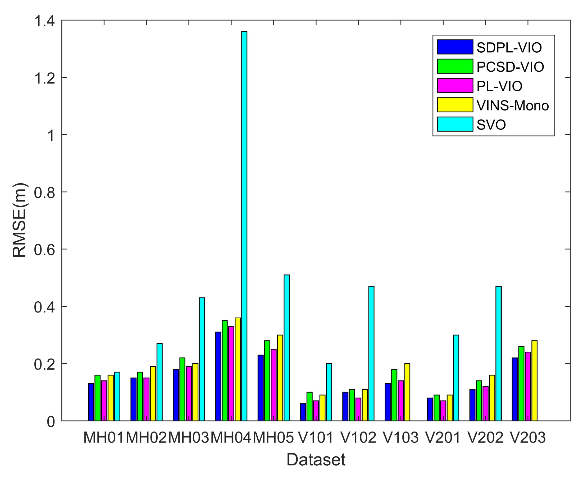
We implemented the above methods on the EuRoC datasets. In order to intuitively reflect the tracking effect of our proposed semi-direct method, and because PL-VIO lacks the loop-closure module, we disabled the loop-closure module of the above methods. A comparison of root–mean–square error (RMSE) on the EuRoC datasets is shown in Table 1, and their histograms are also provided, as shown in Figure 10. Table 1 shows that SDPL-VIO works robustly and accurately, and other methods also work well. Compared with point features, the combination of point and line features can strengthen the constraints between images, are insensitive to illumination changing environment, deal with the dynamic environment, and reduce the error caused by fast rotation motion. Thus, due to the introduction of line features, the accuracy of SDPL-VIO is better than SVO, PCSD-VIO and VINS-Mono, which only uses point features for tracking. In easy sequences such as MH01 and V101, which have rich features, good illumination, and slow motion, the feature-based method can extract a high number of point and line features. In such environments, the quality of tracking is about the same, so the accuracy of SDPL-VIO is comparable to PL-VIO. In difficult sequences, such as MH05, V203 with motion blur, fast motion, low texture, etc., the feature-based method faces challenges due to the lack of sufficient visual features. Our proposed semi-direct method combines the excellent performance of direct methods in low-texture environments. The feature-based method provides an accurate initialization state and generates keyframes that provide good priors for the direct method, while the direct method uses direct image alignment to move the frame very close to its final pose, while using a refinement step to reduce the pose estimation error. Therefore, SDPL-VIO performs relatively well in difficult sequences.
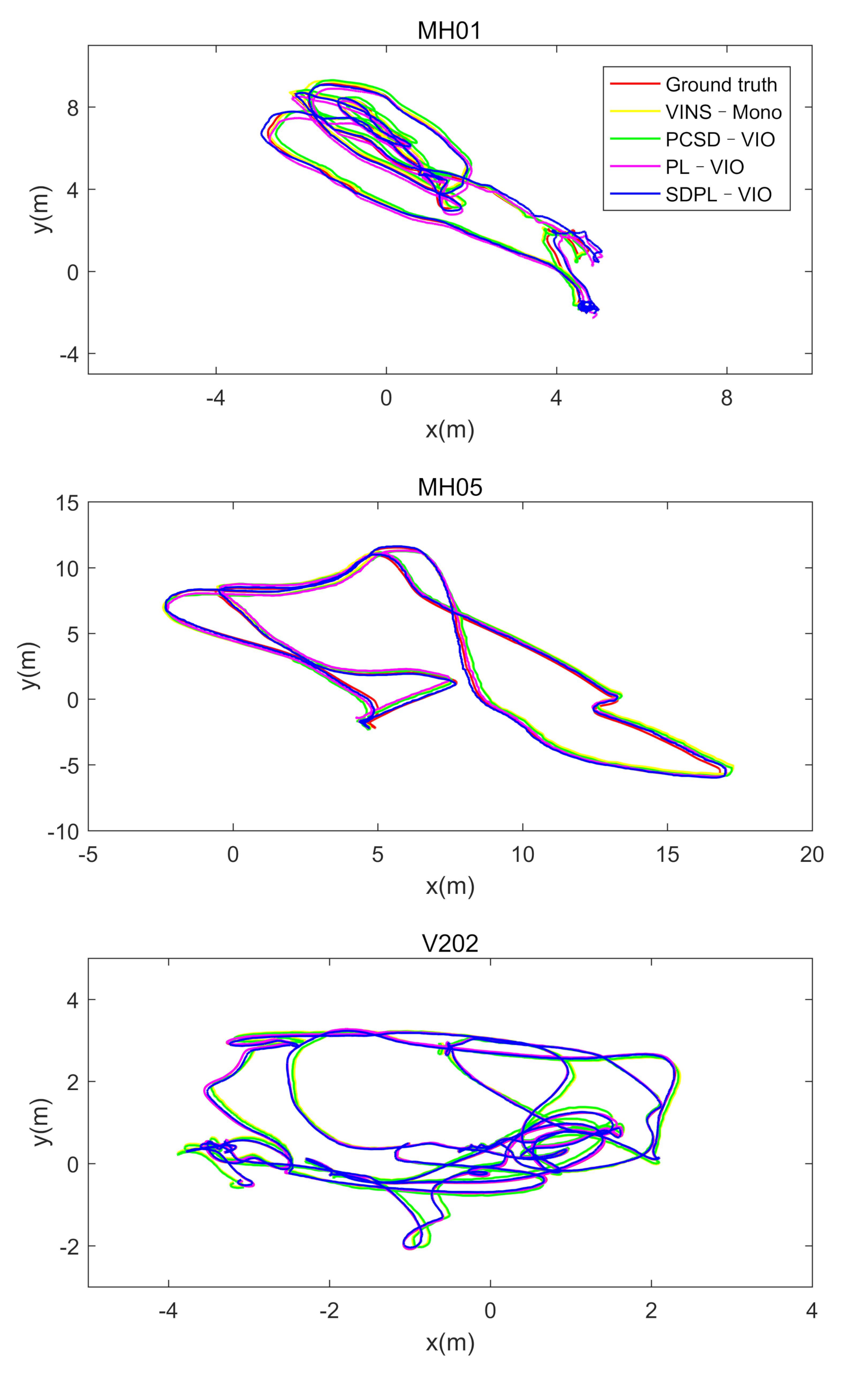
Figure 11 shows a comparison of the trajectories obtained by SDPL-VIO, PCSD-VIO, PL-VIO and VINS-Mono on the MH01, MH05 and V202 datasets, respectively. The ground truth is represented by the red line, while the results of SDPL-VIO, PCSD-VIO, PL-VIO and VINS-Mono are represented by the blue line, the green line, the purple line and the yellow line, respectively.
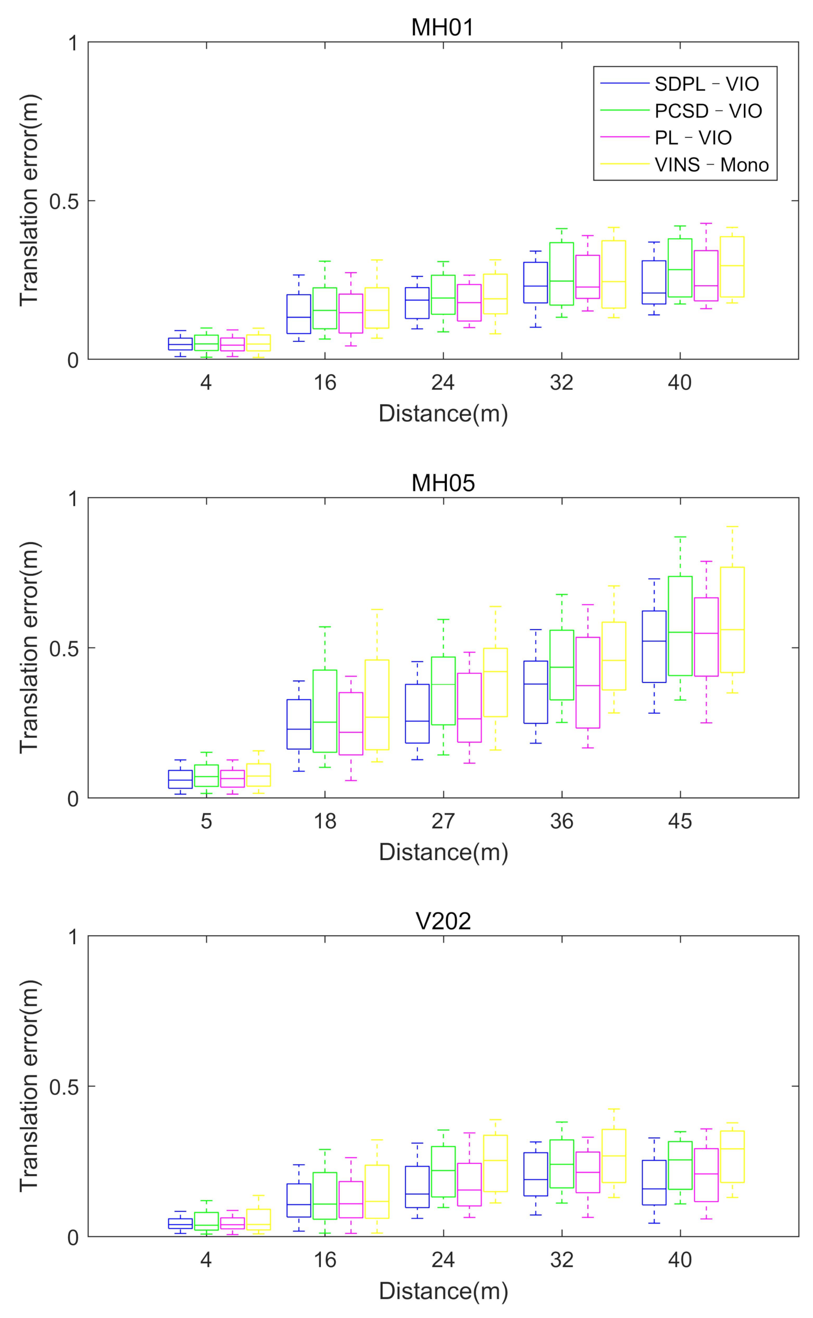
Figure 12 shows the translation errors on the MH01, MH05 and V202 datasets, in which the blue represents SDPL-VIO, the green represents PCSD-VIO, the purple represents PL-VIO, and the yellow represents VINS-Mono. It can been seen that, in the MH01 sequence, due to the rich scene features and good illumination conditions, there is not much difference in the accuracy of the four methods. The maximum error of SDPL-VIO is 0.37 m in the sequence of MH01, while that of PCSD-VIO is 0.41 m, that of PL-VIO is 0.41 m and that of VINS-Mono is 0.40 m, respectively. The MH05 dataset includes fast motion and large illumination changes. The combination of point and line features is more robust to fast rotation in the trajectory, and the semi-direct method is more adaptable to low-texture environments, so SDPL-VIO has the highest accuracy. PCSD-VIO and VINS-Mono only extract point features, and they struggle to extract corner points with large grayscale differences from surrounding pixel blocks. Therefore, the number of effective feature points is reduced, and the accuracy is the lower than the other two methods. The maximum error of SDPL-VIO is 0.73 m in the sequence of MH05, while that of PCSD-VIO is 0.85 m, that of PL-VIO is 0.78 m and that of VINS-Mono is 0.90 m, respectively. For the V202 dataset, SDPL-VIO still performs better than the other three. The maximum error of SDPL-VIO is 0.33 m, while that of PCSD-VIO is 0.37 m, that of PL-VIO is 0.36 m and that of VINS-Mono is 0.42 m, respectively. From Figure 11 and Figure 12, it can been seen that, due to the semi-direct method tracking point and line features, SDPL-VIO has a better performance than the other three methods in challenging sequences, such as fast motion, large illumination changes or poorly textured environments, etc.
4.2. Computational Performance
To evaluate the computational performances of SDPL-VIO, the average times taken for tracking and marginalization were measured and analyzed.
4.2.1. Average Time for Tracking
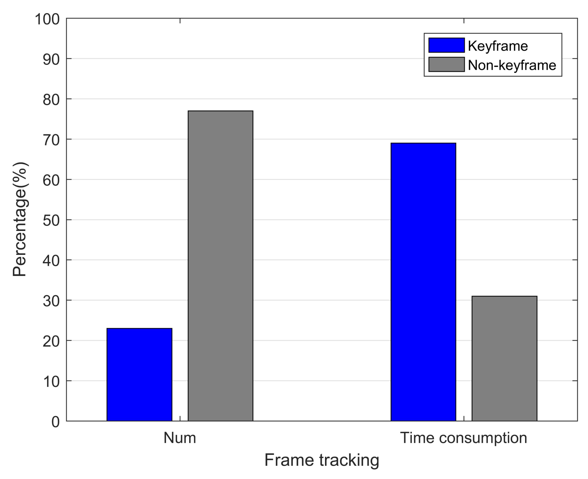
Firstly the computational performances when tracking the image were analyzed to compare SDPL-VIO and PL-VIO, and the comparison results are shown in Table 2. PL-VIO simultaneously extracts point and line features for each frame, which is very time-consuming. SDPL-VIO uses the semi-direct method for tracking, and takes much less time than PL-VIO. This is because non-keyframes account for the majority of the tracked features and the system uses the direct method, with the advantage of rapidity when tracking non-keyframes in the front end, and has no need to extract image features and calculate descriptors. This strategy effectively reduces the average front-end tracking time. Taking V201 as an example, as shown in Figure 13, according to the keyframe selection strategy, the number of selected keyframes is 127, accounting for about 23% of the total frames, while 77% of the frames were selected to be non-keyframes. However, the time needed to track keyframes accounted for 69% of the total time, while the time needed to track non-keyframes accounted for only 31%. Although the tracking time was reduced, the accuracy of SDPL-VIO was not significantly reduced; this was still comparable with PL-VIO, and even higher in some environments, as shown in Section 4.1.
4.2.2. Average Time for Marginalization
Marginalization is another time-consuming aspect of the back-end, so the average time consumption was also analyzed. Taking V102 as an example, as explained in Section 3.3.2, when the back end of SDPL-VIO used the basic marginalization method, one-step marginalization was carried out, resulting in a very large amount of computation, and the average time needed for marginalization was 39 ms. When the back end used the improved marginalization method, the high-dimension matrix corresponding to the cost function was decomposed step by step. Therefore, the amount of computation was significantly reduced, and the average time needed for marginalization was 16 ms.
4.3. Loop Closure Detection Evaluation
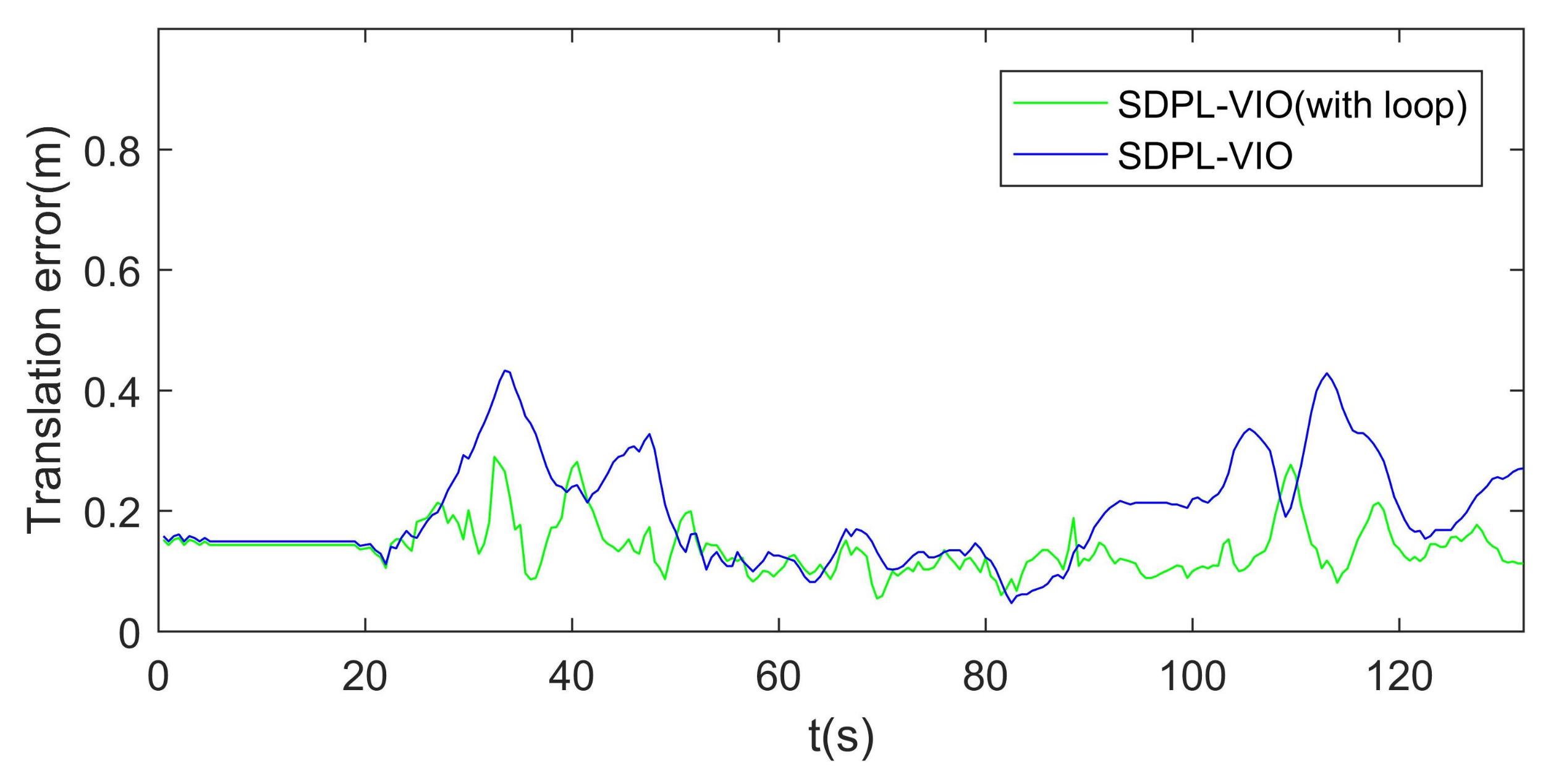
The most obvious advantage of the feature-based method compared with the direct method is that the feature-based method could be used for loop closure detection, which can reduce the drift accumulated during the long-term operation. Therefore, the loop-closure detection ability of SDPL-VIO was finally evaluated to verify the integrity and reliability of the system. From the comparison results on the MH03 dataset, as shown in Figure 14, the accuracy of SDPL-VIO with loop closure detection is clearly shown to improve.
The analysis of multiple experiments shows that SDPL-VIO can consider both speed and accuracy, which increases the operation efficiency without reducing the operation precision, and is superior to other methods in terms of comprehensive performance.
5. Conclusions
In this paper, a novel, semi-direct, point-line, visual inertial odometry for MAVs was proposed, which extracts point-line features from the image and uses the semi-direct method to track keyframes and non-keyframes. The proposed method also adopts the sliding window strategy and uses the improved marginalization method to decompose the high-dimensional matrix step by step, according to the cost function, to optimize the solution. Experiments on the EuRoC datasets show that the accuracy and real-time performance of SDPL-VIO is better than that of other state-of-the-art VIO methods, especially in challenging datasets containing fast motion, large illumination changes or poorly textured environments. The SDPL-VIO performance, in terms of accuracy and efficiency, validated that it is suitable for navigational uses in MAVs with low-cost sensors. In future work, we aim to adopt a faster line detector that could be more conducive to continuous and real-time tracking.
Author Contributions
Conceptualization, B.G., B.L. and C.T.; Formal analysis, B.G. and C.T.; Investigation, B.G.; Methodology, B.G. and C.T.; Project administration, B.L.; Resources, B.L.; Software, B.G. and C.T.; Supervision, B.L.; Validation, B.G.; Writing—original draft, B.G.; Writing—review & editing, B.G. and C.T. All authors have read and agreed to the published version of the manuscript.
Funding
This work was supported in part by National Natural Science Foundation of China under Grant 62171735, 62271397, 62173276, 62101458, 61803310 and 61801394, in part by the Natural Science Basic Research Program of Shaanxi under Grant 2022GY-097, 2021JQ-122 and 2021JQ-693, and in part by China Postdoctoral Science Foundation under Grant 2020M673482 and 2020M673485.
Institutional Review Board Statement
Not applicable.
Informed Consent Statement
Not applicable.
Data Availability Statement
Not applicable.
Conflicts of Interest
The authors declare no conflict of interest.
Abbreviations
The following abbreviations are used in this manuscript:
| MAVs | Micro Aerial Vehicles |
| IMU | Inertial Measurement Unit |
| VIO | Visual Inertial Odometry |
| VIN | Visual Inertial Navigation |
| OKVIS | Keyframe-based visual-inertial SLAM using nonlinear optimization |
| BRISK | BRISK: Binary robust invariant scalable keypoints |
| ORB | Oriented FAST and Rotated BRIEF |
| ORB-SLAM2 | ORB-SLAM2: An Open-Source SLAM System for Monocular, Stereo, and |
| RGB-D Cameras | |
| PL-SLAM | PL-SLAM: Real-time monocular visual SLAM with points and lines |
| DSO | Direct Sparse Odometry |
| VINS-Mono | VINS-Mono: A Robust and Versatile Monocular Visual-Inertial State Estimator |
| PL-VIO | PL-VIO: Tightly-Coupled Monocular Visual–Inertial Odometry Using Point and |
| Line Features | |
| SVO | SVO: Fast semi-direct monocular visual odometry |
| PL-SVO | PL-SVO: Semi-direct Monocular Visual Odometry by combining points and |
| line segments | |
| SVL | Semi-direct monocular visual and visual-inertial SLAM with loop closure detection |
| PCSD-VIO | PC-SD-VIO: A constant intensity semi-direct monocular visual-inertial odometry |
| with online photometric calibration | |
| EuRoC | the European Robotics Challenge |
| SFM | Structure from Motion |
| FAST | the Accelerated Segment Test |
| KLT | Kanade-Lucas-Tomasi |
| RANSAC | Random Sample Consensus |
| LSD | Line Segment Detector |
| LBD | Line Band Descriptors |
| DBoW2 | Bags of Words |
| RMSE | root-mean-square error |
References
- Citroni, R.; Di Paolo, F.; Livreri, P. A Novel Energy Harvester for Powering Small UAVs: Performance Analysis, Model Validation and Flight Results. Sensors 2019, 19, 1771. [Google Scholar] [CrossRef]
- Delmerico, J.; Scaramuzza, D. A Benchmark Comparison of Monocular Visual-Inertial Odometry Algorithms for Flying Robots. In Proceedings of the IEEE International Conference on Robotics and Automation (ICRA), Brisbane, Australia, 21–25 May 2018; pp. 2502–2509. [Google Scholar]
- Cheng, J.; Zhang, L.; Chen, Q.; Hu, X.; Cai, J. A review of visual SLAM methods for autonomous driving vehicles. Eng. Appl. Artif. Intell. 2022, 114, 104992. [Google Scholar] [CrossRef]
- Mourikis, A.I.; Roumeliotis, S.I. A Multi-State Constraint Kalman Filter for Vision-aided Inertial Navigation. In Proceedings of the IEEE International Conference on Robotics and Automation (ICRA), Rome, Italy, 10–14 April 2007; pp. 3565–3572. [Google Scholar]
- Leutenegger, S.; Lynen, S.; Bosse, M.; Siegwart, R.; Furgale, P. Keyframe-based visual-inertial odometry using nonlinear optimization. Int. J. Robot. Res. 2014, 34, 314–334. [Google Scholar] [CrossRef]
- Bloesch, M.; Omari, S.; Hutter, M.; Siegwart, R. Robust visual inertial odometry using a direct EKF-based approach. In Proceedings of the IEEE/RSJ International Conference on Intelligent Robots and Systems (IROS), Hamburg, Germany, 28 September–2 October 2015; pp. 298–304. [Google Scholar]
- Mur-Artal, R.; Tardós, J.D. ORB-SLAM2: An Open-Source SLAM System for Monocular, Stereo, and RGB-D Cameras. IEEE Trans. Robot. 2017, 33, 1255–1262. [Google Scholar] [CrossRef]
- Pumarola, A.; Vakhitov, A.; Agudo, A.; Sanfeliu, A.; Moreno-Noguer, F. PL-SLAM: Real-time monocular visual SLAM with points and lines. In Proceedings of the IEEE International Conference on Robotics and Automation (ICRA), Singapore, 29 May–3 June 2017; pp. 4503–4508. [Google Scholar]
- Mur-Artal, R.; Tardós, J.D. Visual-Inertial Monocular SLAM With Map Reuse. IEEE Robot. Autom. Lett. 2017, 2, 796–803. [Google Scholar] [CrossRef]
- Qin, T.; Li, P.; Shen, S. VINS-Mono: A Robust and Versatile Monocular Visual-Inertial State Estimator. IEEE Trans. Robot. 2018, 34, 1004–1020. [Google Scholar] [CrossRef]
- He, Y.; Zhao, J.; Guo, Y.; He, W.; Yuan, K. PL-VIO: Tightly-Coupled Monocular Visual–Inertial Odometry Using Point and Line Features. Sensors 2019, 18, 1159. [Google Scholar] [CrossRef]
- Duan, R.; Paudel, D.P.; Fu, C.; Lu, P. Stereo Orientation Prior for UAV Robust and Accurate Visual Odometry. IEEE/ASME Trans. Mechatronics 2022, 1–11. [Google Scholar] [CrossRef]
- Engel, J.; Schps, T.; Cremers, D. LSD-SLAM: Large-Scale Direct Monocular SLAM; Springer: Cham, Switzerland, 2014. [Google Scholar]
- Engel, J.; Koltun, V.; Cremers, D. Direct Sparse Odometry. IEEE Trans. Pattern Anal. Mach. Intell. 2018, 40, 611–625. [Google Scholar] [CrossRef]
- Forster, C.; Pizzoli, M.; Scaramuzza, D. SVO: Fast semi-direct monocular visual odometry. In Proceedings of the IEEE International Conference on Robotics and Automation (ICRA), Hong Kong, China, 31 May–7 June 2014. [Google Scholar]
- Gomez-Ojeda, R.; Briales, J.; Gonzalez-Jimenez, J. PL-SVO: Semi-direct Monocular Visual Odometry by combining points and line segments. In Proceedings of the 2016 IEEE/RSJ International Conference on Intelligent Robots and Systems (IROS), Daejeon, Korea, 9–14 October 2016; pp. 4211–4216. [Google Scholar]
- Forster, C.; Zhang, Z.; Gassner, M.; Werlberger, M.; Scaramuzza, D. SVO: Semidirect Visual Odometry for Monocular and Multicamera Systems. IEEE Trans. Robot. 2017, 33, 249–265. [Google Scholar] [CrossRef] [Green Version]
- Li, S.; Zhang, T.; Gao, X.; Wang, D.; Xian, Y. Semi-direct monocular visual and visual-inertial SLAM with loop closure detection. Robot. Auton. Syst. 2019, 112, 201–210. [Google Scholar] [CrossRef]
- Lee, S.H.; Civera, J. Loosely-Coupled Semi-Direct Monocular SLAM. IEEE Robot. Autom. Lett. 2019, 4, 399–406. [Google Scholar] [CrossRef]
- Dong, X.; Cheng, L.; Peng, H.; Li, T. FSD-SLAM: A fast semi-direct SLAM algorithm. Complex Intell. Syst. 2021, 8, 1823–1834. [Google Scholar] [CrossRef]
- Luo, H.; Pape, C.; Reithmeier, E. Hybrid Monocular SLAM Using Double Window Optimization. IEEE Robot. Autom. Lett. 2021, 6, 4899–4906. [Google Scholar] [CrossRef]
- Liu, Q.; Wang, Z.; Wang, H. PC-SD-VIO: A constant intensity semi-direct monocular visual-inertial odometry with online photometric calibration. Robot. Auton. Syst. 2021, 146, 103877. [Google Scholar] [CrossRef]
- Usenko, V.; Demmel, N.; Schubert, D.; Stueckler, J.; Cremers, D. Visual-Inertial Mapping with Non-Linear Factor Recovery. IEEE Robot. Autom. Lett. (RA-L) Int. Intell. Robot. Autom. (ICRA) 2020, 5, 422–429. [Google Scholar] [CrossRef]
- Xiao, J.; Xiong, D.; Yu, Q.; Huang, K.; Lu, H.; Zeng, Z. A Real-Time Sliding Window based Visual-Inertial Odometry for MAVs. IEEE Trans. Ind. Inform. 2020, 16, 4049–4058. [Google Scholar] [CrossRef]
- Guan, Q.; Wei, G.; Wang, L.; Song, Y. A Novel Feature Points Tracking Algorithm in Terms of IMU-Aided Information Fusion. IEEE Trans. Ind. Inform. 2021, 17, 5304–5313. [Google Scholar] [CrossRef]
- Xu, C.; Liu, Z.; Li, Z. Robust Visual-Inertial Navigation System for Low Precision Sensors under Indoor and Outdoor Environments. Remote Sens. 2021, 13, 772. [Google Scholar] [CrossRef]
- Stumberg, L.v.; Cremers, D. DM-VIO: Delayed Marginalization Visual-Inertial Odometry. IEEE Robot. Autom. Lett. 2022, 7, 1408–1415. [Google Scholar] [CrossRef]
- Sibley, G.; Matthies, L.; Sukhatme, G. Sliding window filter with application to planetary landing. J. Field Robot. 2010, 27, 587–608. [Google Scholar] [CrossRef]
- Bartoli, A.; Sturm, P. The 3D line motion matrix and alignment of line reconstructions. In Proceedings of the IEEE Computer Society Conference on Computer Vision and Pattern Recognition, CVPR 2001, Kauai, HI, USA, 8–14 December 2001; pp. 287–292. [Google Scholar]
- Bartoli, A.; Sturm, P. Structure-From-Motion Using Lines: Representation, Triangulation and Bundle Adjustment. Comput. Vis. Image Underst. 2005, 100, 416–441. [Google Scholar] [CrossRef]
- Rosten, E.; Porter, R.; Drummond, T. Faster and Better: A Machine Learning Approach to Corner Detection. IEEE Trans. Pattern Anal. Mach. Intell. 2010, 32, 105–119. [Google Scholar] [CrossRef]
- Lucas, B.D.; Kanade, T. An iterative image registration technique with an application to stereo vision. In Proceedings of the Imaging Understanding Workshop, Vancouver, BC, Canada, 24–28 August 1981; pp. 121–130. [Google Scholar]
- Gioi, R.; Jakubowicz, J.; Morel, J.M.; Randall, G. LSD: A Fast Line Segment Detector with a False Detection Control. IEEE Trans. Pattern Anal. Mach. Intell. 2010, 32, 722–732. [Google Scholar] [CrossRef]
- Zhang, L.; Koch, R. An efficient and robust line segment matching approach based on LBD descriptor and pairwise geometric consistency. J. Vis. Commun. Image Represent. 2013, 24, 794–805. [Google Scholar] [CrossRef]
- Galvez-Lopez, D.; Tardos, J.D. Bags of Binary Words for Fast Place Recognition in Image Sequences. IEEE Trans. Robot. 2012, 28, 1188–1197. [Google Scholar] [CrossRef]
- Burri, M.; Nikolic, J.; Gohl, P.; Schneider, T.; Rehder, J.; Omari, S.; Achtelik, M.W.; Siegwart, R. The EuRoC micro aerial vehicle datasets. Int. J. Robot. Res. 2016, 35, 1157–1163. [Google Scholar] [CrossRef]
Figure 1.
The system framework.

Figure 2.
Direct image alignment.

Figure 3.
Pose refinement.

Figure 4.
Illustration of the visual reprojection errors.

Figure 5.
Illustration of marginalization.

Figure 6.
States in the sliding window.

Figure 7.
The Hessian matrix corresponding to Equation (24).
Figure 7.
The Hessian matrix corresponding to Equation (24).

Figure 8.
The Hessian matrix after marginalization of .

Figure 9.
The Hessian matrix after the marginalization of all landmarks.

Figure 10.
RMSE (m) of the five methods.

Figure 11.
The comparison of trajectories on the MH01, MH05 and V202 datasets.

Figure 12.
The comparison of translation errors on the MH01, MH05 and V202 datasets.

Figure 13.
The ratio of the number and tracking time between keyframes and non-keyframes on the V201 dataset.
Figure 13.
The ratio of the number and tracking time between keyframes and non-keyframes on the V201 dataset.

Figure 14.
The comparison of translation errors on the MH03 dataset.


Table 1.
RMSE (m) of the five methods.
| Sequence | SDPL-VIO | PCSD-VIO | PL-VIO | VINS-Mono | SVO |
|---|---|---|---|---|---|
| MH01 | 0.13 | 0.16 | 0.14 | 0.16 | 0.17 |
| MH02 | 0.15 | 0.17 | 0.15 | 0.19 | 0.27 |
| MH03 | 0.18 | 0.22 | 0.19 | 0.20 | 0.43 |
| MH04 | 0.31 | 0.35 | 0.33 | 0.36 | 1.36 |
| MH05 | 0.23 | 0.28 | 0.25 | 0.30 | 0.51 |
| V101 | 0.06 | 0.10 | 0.07 | 0.09 | 0.20 |
| V102 | 0.10 | 0.11 | 0.08 | 0.11 | 0.47 |
| V103 | 0.13 | 0.18 | 0.14 | 0.20 | N/A |
| V201 | 0.08 | 0.09 | 0.07 | 0.09 | 0.30 |
| V202 | 0.11 | 0.14 | 0.12 | 0.16 | 0.47 |
| V203 | 0.22 | 0.26 | 0.24 | 0.28 | N/A |
Table 2.
Average time (ms) spent tracking an image.
| Sequence | SDPL-VIO | PL-VIO |
|---|---|---|
| MH01 | 28.54 | 84.40 |
| MH02 | 33.55 | 88.05 |
| MH03 | 27.51 | 85.73 |
| MH04 | 30.45 | 83.18 |
| MH05 | 30.10 | 83.10 |
| V101 | 29.65 | 82.52 |
| V102 | 29.48 | 83.35 |
| V103 | 32.81 | 87.61 |
| V201 | 30.15 | 81.24 |
| V202 | 31.65 | 89.76 |
| V203 | 33.56 | 90.40 |
Publisher’s Note: MDPI stays neutral with regard to jurisdictional claims in published maps and institutional affiliations. |
© 2022 by the authors. Licensee MDPI, Basel, Switzerland. This article is an open access article distributed under the terms and conditions of the Creative Commons Attribution (CC BY) license (https://creativecommons.org/licenses/by/4.0/).
Share and Cite
MDPI and ACS Style
Gao, B.; Lian, B.; Tang, C. Semi-Direct Point-Line Visual Inertial Odometry for MAVs. Appl. Sci. 2022, 12, 9265. https://doi.org/10.3390/app12189265
AMA Style
Gao B, Lian B, Tang C. Semi-Direct Point-Line Visual Inertial Odometry for MAVs. Applied Sciences. 2022; 12(18):9265. https://doi.org/10.3390/app12189265
Chicago/Turabian StyleGao, Bo, Baowang Lian, and Chengkai Tang. 2022. "Semi-Direct Point-Line Visual Inertial Odometry for MAVs" Applied Sciences 12, no. 18: 9265. https://doi.org/10.3390/app12189265
Note that from the first issue of 2016, this journal uses article numbers instead of page numbers. See further details here.