A Reversible Hydropump–Turbine System

Abstract

Water-pumped storage systems have become an ideal alternative to regulate the intermittent power delivered by renewable energy sources. For small-scale operations, a type of centrifugal pump coupled to asynchronous machines represents an adequate solution due to their techno-economic feasibility in addition to their ability to operate as reversible systems. This work provides a novel port-Hamiltonian modelling approach to an integrated reversible hydropump–turbine system, that can be switched from motor pump to turbine-generator by employing a conventional hydraulic switch. Our modelling strategy provides a clear physical interpretation of the energy flow from the mechanical to electrical domains. Then, the model was built with multi-domain storing and dissipating elements and the interconnection of well-defined input–output port pairs. The system’s internal energy, i.e., Hamiltonian function, can be exploited for energy-shaping control strategies. The performance of our modelling approach is validated via numerical simulations.

1. Introduction

The increase in the worldwide energy demand due to population and productive growth motivates the search for alternative renewable energy sources. However, intermittent renewable energy sources, such as solar- and wind-based sources, have fluctuating and unpredictable behaviours, which limit their optimal performance to supply electrical power continuously. In order to tackle the aforementioned issue, the design and implementation of bulk energy storage are required [1]. More specifically, hydraulic (mechanical) energy storage by pumping water from a lower to an upper reservoir is presented as a potential solution when the infrastructure and topography are adequate [2]. The storing-generating system should be able to switch from the pump to turbine modes efficiently [2]. Storing the energy in hydraulic repositories improves grid stability and facilitates the deployment of intermittent renewable energy sources [1].

We make use of a type of centrifugal pump together with a squirrel cage induction motor due to their wide operating range and low maintenance cost. In [3], a review of the state-of-the-art on pumps running as a turbine is carried out. Such a study concludes that a single-stage centrifugal pump is the configuration most recommended by researchers to operate in the turbine mode due to the techno-economic considerations.

To maximize the application of reversible pump–turbine systems in power generation, mathematical modelling strategies are necessary to adequately and simply describe the physical behaviour of this system. Such modelling approaches should allow subsystems in different domains (electrical, mechanical, and hydraulic) to be easily coupled to each other, in addition to facilitating the design of efficient control strategies.

Several models of centrifugal pumps with their advantages and disadvantages are recapitulated by [4]. For instance, in [5], the general model of a solar-powered centrifugal pump connected to an induction motor was introduced with a type of equivalent circuit optimization technique. The work of [6] suggests a modelling approach to a centrifugal pump system where its input pressure depends directly on a quadratic form of its rotational speed. The description of pumped storage systems found in [7] presents second-order differential equations that consider the pump–turbine’s nonlinearities. Furthermore, in [8], a model of variable speed doubly-fed induction-generator pumped storage power is presented, which is described as a nonlinear eighth-order state equation with eight state variables. Moreover, a five-order nonlinear dynamic system of the variable-speed pumped storage power station was developed in [9], while in [10], a variable-speed pumped storage model is shown via algebraic differential equations. In addition to the above mentioned examples, a nonlinear model of a water distribution network based on a port-Hamiltonian description is presented in [11]. Moreover, a Hamiltonian model of a hydro-power system is presented in [12], which provides a theoretical basis for its safe and stable operation during transient processes. Such a model is used later on in [13] where a passivity-based control is designed. Their control strategy guarantees stability and efficient performance under different operating conditions. In [14], an energy-based modelling approach is developed where a solar-powered hydro pump system is coupled to a direct current motor. A model based on a port-Hamiltonian approach to an asynchronous motor is introduced by [15,16], and later on extended to the modelling of an asynchronous machine configured as a generator by [17]. A trajectory tracking control strategy for the system in [17] is presented in [18]. Finally, in [11], a controller for a water-distribution system is designed, using a port-Hamiltonian approach to model the pump, allowing them to analyze stability, including nonlinear elements.

Here, we make use of the port-Hamiltonian formalism where the emphasis to the power balance of the system with its storing and dissipating elements are key to understanding how the energy flows from one physical domain to another. The port-Hamiltonian approach depends on well-defined power port-pairs that facilitate energy exchange per domain. The formalism introduced by [19,20] is a Hamiltonian systems generalization with structure preservation properties that allows modelling and the design of controllers using energy shaping and damping injections. Under this framework, the structure preservation also renders an asymptotically stable closed-loop system even with significant parameter uncertainties for a wide variety of nonlinear systems [21,22].

The main contribution of this work is related to a generalization of the integrated reversible hydropump–turbine system model based on the port-Hamiltonian modelling approach. The physical elements of the system’s range from a lower and upper reservoir to a penstock and a centrifugal pump that can be configured as a turbine. We make use of an approach based on energy due to the multi-domain characteristics of our proposed system that consists of hydraulic-, electric-, and mechanical-storing and dissipating elements. Finally, the selection of the pump or turbine operation is performed via a conventional hydraulic switch. This novel modelling approach will allow the development of trajectory tracking and energy-based controllers for small- and medium-scale hydropump generation systems.

The structure of this paper follows five different sections. In Section 2, a port-Hamiltonian framework with its benefits in structure preservation properties, energy storage, and energy dissipation is introduced. A newfangled model relative to the reversible pump–turbine system that includes a centrifugal pump and an asynchronous machine is presented in Section 3 using a port-Hamiltonian modelling approach. In Section 4, we validate the proposed modelling approach of our reversible system via simulation results. Finally, in Section 5, we provide our main concluding remarks and future research directions.

2. Preliminaries

Firstly, we cover the bases of the port-Hamiltonian modelling framework of [19,20] from which the modeling approach for the dual pump–turbine system is inspired.

Port-Hamiltonian Framework

We first recapitulate the port-Hamiltonian (PH) framework for a general class of (non)linear physical systems. It describes the interconnection structure, dissipating elements, inputs and outputs related to power port pairs, and the energy function called Hamiltonian. Via the PH formalism, we can model and control (non)linear hydraulic, electrical, mechanical, electro-mechanical, and thermal systems. The clarity with which power-preserving ports, dissipation, and energy-storage components is modeled involves energy transfers between the physical system and the environment and characterizes the PH framework [19,20].

A PH system corresponds (we assume ${\displaystyle \frac{\partial H\left(x\right)}{\partial x}}={\nabla }_{x}H\left(x\right)$ without a loss of generality along this document) to the following:

$${\mathrm{\Sigma }}_{PH}\left\{\begin{array}{cc}\dot{x}\hfill & =\left[J\left(x\right)-R\left(x\right)\right]{\nabla }_{x}H\left(x\right)+g\left(x\right)u,\hfill \\ y\hfill & =g{\left(x\right)}^{\top }{\nabla }_{x}H\left(x\right),\hfill \end{array}\right.$$

(1)

where $x\in {\mathbb{R}}^{\mathcal{N}}$ is the state variable, and $u\in {\mathbb{R}}^{\mathcal{M}}$ and $y\in {\mathbb{R}}^{\mathcal{M}}$ are the input–output port pair representing flows and efforts, respectively. In addition, the input, dissipation, and interconnection matrices of (1) are given by the following:

$$\begin{array}{}\mathrm{(2)}& \begin{array}{cc}g\left(x\right)\hfill & \in {\mathbb{R}}^{\mathcal{N}\times \mathcal{M}},\hfill \end{array}\hfill \mathrm{(3)}& \begin{array}{cc}J\left(x\right)\hfill & =-J{\left(x\right)}^{\top },J\left(x\right)\in {\mathbb{R}}^{\mathcal{N}\times \mathcal{N}},\hfill \end{array}\hfill \mathrm{(4)}& \begin{array}{cc}R\left(x\right)\hfill & =R{\left(x\right)}^{\top }\succcurlyeq 0,R\left(x\right)\in {\mathbb{R}}^{\mathcal{N}\times \mathcal{N}},\hfill \end{array}\hfill \end{array}$$

where $\mathcal{M}\le \mathcal{N}$. In a mechanical system, when $\mathcal{M}=\mathcal{N}$, the system is fully actuated, and it is under-actuated if $\mathcal{M}<\mathcal{N}$. The function $H\left(x\right)\in \mathbb{R}$ is the energy of system, where the Hamiltonian is obtained along the trajectories of $\dot{x}$ as in (1). The time differentiation of $H\left(x\right)$ allows a recovery energy balance that is described as follows.

$$\dot{H}\left(x\right)=-{\nabla }_x^{\top }H\left(x\right)R\left(x\right){\nabla }_{x}H\left(x\right)+{\nabla }_{t}H\left(x\right)+y^{\top }u\le y^{\top }u.$$

(5)

The system (1) would be clearly conservative if $\dot{H}\left(x\right)=y^{\top }u$, as well as passive when $\dot{H}\left(x\right)\le y^{\top }u$.

Since we already introduced a general PH approach, the energy-based modelling of the asynchronous machine configured as a motor and generator follows.

3. An Energy-Based Model Relative to the Reversible Hydropump–Turbine System

This section provides a general description of our reversible hydropump–turbine system. First, a model of a three-phase induction motor and the centrifugal pump is provided by considering their coupled hydraulic and mechanical domains. Furthermore, the reverse mode as a turbine-generator is provided. Finally, the two systems are coupled into a single generalized model for the reversible hydro pump-turbine system. The modelling approach is made in the PH framework such that the interconnection and dissipation elements are clearly shown together with the input–output portpairs.

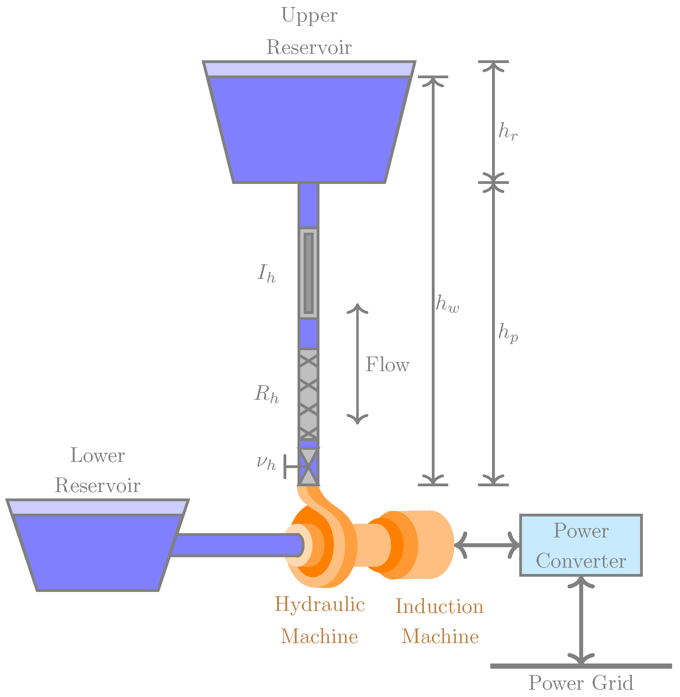
3.1. System’s Architecture

The reversible hydro pump-turbine system under study is shown in Figure 1, which consists of a centrifugal pump driven by an induction motor. The hydropumping action is meant to store potential energy by pumping water from a lower to an upper reservoir. The induction motor is able to elevate a column of water via a penstock and hydraulic valve ${\nu }_h$, which is connected to the bottom of the upper reservoir. It is assumed that electrical power is provided to the induction motor via an AC grid or a DC grid in addition to power converters. Finally, the centrifugal pump behaves as a turbine when the water in the upper reservoir is used to generate and provide electrical power to the same AC or DC grid that previously actuated the asynchronous motor. The turbine actuates the asynchronous machine, which is now configured as a generator.

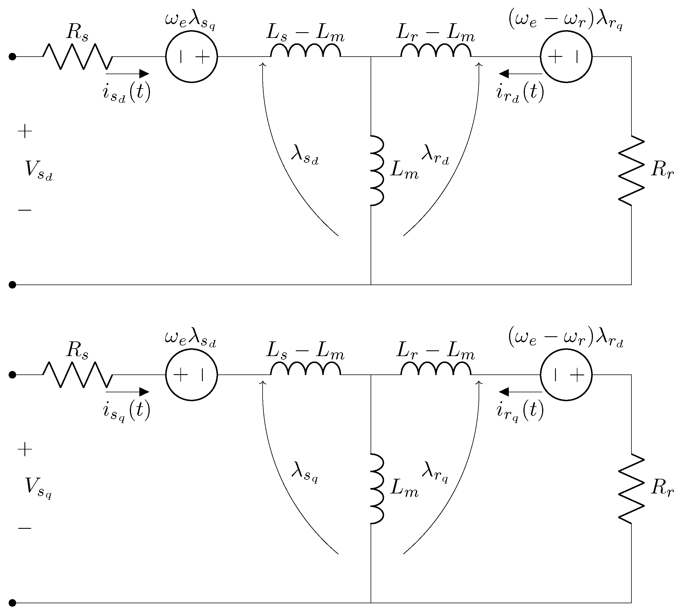
3.2. Motor Configuration of the Asynchronous Machine

In the Figure 2, the asynchronous machine model configured as a motor is presented as in [15,16,23,24] in the d-q axis so the parameters of time dependence have been rewritten in direct and quadrature axes. Consequently, the explicit time-dependent variable is not presented anymore. We recapitulate here the PH modelling approach relative to the asynchronous machine configured as a motor and generator previously published in [17]. The nonlinear dynamics of the asynchronous motor are described as follows:

$$\begin{array}{}\mathrm{(6)}& \begin{array}{cc}\hfill {\dot{\lambda }}_{s_d}& ={\omega }_e{\lambda }_{s_q}+V_{s_d}-R_s{i}_{s_d},\hfill \end{array}\hfill \mathrm{(7)}& \begin{array}{cc}\hfill {\dot{\lambda }}_{s_q}& =-{\omega }_e{\lambda }_{s_d}+V_{s_q}-R_s{i}_{s_q},\hfill \end{array}\hfill \mathrm{(8)}& \begin{array}{cc}\hfill {\dot{\lambda }}_{r_d}& =({\omega }_e-{\omega }_r){\lambda }_{r_q}+V_{r_d}-R_r{i}_{r_d},\hfill \end{array}\hfill \mathrm{(9)}& \begin{array}{cc}\hfill {\dot{\lambda }}_{r_q}& =-({\omega }_e-{\omega }_r){\lambda }_{r_d}+V_{r_q}-R_r{i}_{r_q},\hfill \end{array}\hfill \mathrm{(10)}& \begin{array}{cc}\hfill {\dot{p}}_M& =\delta n_p{\lambda }_r^{\top }{J}_2{i}_r-R_{m_M}{\omega }_m-{\tau }_L,\hfill \end{array}\hfill \end{array}$$

where state variable $p_M\in \mathbb{R}$$\left[\mathrm{kg}{\mathrm{m}}^2/\mathrm{s}\right]$ represents the generalized momentum. The stator and rotor vector fluxes are given, respectively, by ${\lambda }_s=\mathrm{col}\left({\lambda }_{s_d},{\lambda }_{s_q}\right)$ and ${\lambda }_r=\mathrm{col}\left({\lambda }_{r_d},{\lambda }_{r_q}\right)$, where ${\lambda }_s\in {\mathbb{R}}^{2\times 1}$$\left[\mathrm{Wb}\right]$, ${\lambda }_r\in {\mathbb{R}}^{2\times 1}$$\left[\mathrm{Wb}\right]$, and $J_2$ is a skew-symmetric matrix such that the following is the case.

$$J_2=\left[\begin{array}{cc}0& -1\\ 1& 0\end{array}\right].$$

(11)

Furthermore, in (6)–(10), we have $V_{s_d},V_{s_q},V_{r_d},V_{r_q}\left[V\right]$ and $i_{s_d},i_{s_q},i_{r_d},i_{r_q}\left[A\right]$, which are the stator and rotor voltages and currents for each axis, respectively. Moreover, ${\omega }_r[\mathrm{rad}/\mathrm{s}]$, ${\omega }_e[\mathrm{rad}/\mathrm{s}]$, and ${\omega }_m[\mathrm{rad}/\mathrm{s}]$ are the rotor, synchronous, and mechanical shaft velocities, respectively. In addition to this, the system’s dissipation factors, i.e., the stator and rotor resistances and the rotor friction coefficient, are given by passive elements $R_s\left[\Omega \right]$, $R_r\left[\Omega \right]$, and $R_{m_M}\left[\mathrm{kg}{\mathrm{m}}^2/\mathrm{s}\right]$. ${\tau }_L\left[Nm\right]$ is the torque input to the mechanical shaft. The electrical domain’s active elements are represented by the stator and rotor self-inductance $L_s\left[\mathrm{H}\right]$ and $L_r\left[\mathrm{H}\right]$, respectively, and the rotor and stator mutual-inductances $L_m\left[\mathrm{H}\right]$. Moreover, the number of pole pairs of the system is represented by $n_p$, and a constant rotational inertia $J_{m_M}\left[\mathrm{kg}{\mathrm{m}}^2\right]$ from the mechanical domain. Finally, the stator voltage is given by $V_s\left[\mathrm{V}\right]$, while $V_r=0\left[\mathrm{V}\right]$ represents the rotor’s voltage for a squirrel-cage induction motor. In

Table 1. Key parameters of the reversible hydropump–turbine system.

Parameter	Symbol	Value
IM Stator resistance	$R_s$	1.115 $\left(\mathrm{\Omega }\right)$
IN Rotor resistance	$R_r$	1.083 $\left(\mathrm{\Omega }\right)$
IM Stator inductance	$L_s$	0.20965 $\left(\mathrm{H}\right)$
IM Rotor inductance	$L_r$	0.20965 $\left(\mathrm{H}\right)$
IM Magnetization inductance	$L_m$	0.2037 $\left(\mathrm{H}\right)$
IM Number of pole pairs	$n_p$	2
IM Rotational inertia	$J_{m_M}$	0.02 $\left(\mathrm{kg}{\mathrm{m}}^2\right)$
IM Rotor friction coefficient	$R_{m_M}$	0.005752 $\left(\mathrm{kg}{\mathrm{m}}^2/\mathrm{s}\right)$
IM Nominal voltage	$V_s$	460 $\left({\mathrm{V}}_{\mathrm{rms}}\right)$
IM Operating frequency	f	60 $\left(\mathrm{Hz}\right)$
IM Mechanical speed	${\omega }_m$	1750 $\left(\mathrm{rpm}\right)$
IM Number of phases factor	$\delta$	${ }^3/2$
Pump rotational inertia	$J_{m_P}$	0.008 $\left(\mathrm{kg}{\mathrm{m}}^2\right)$
Pump friction coefficient	$R_{m_P}$	0.005752 $\left(\mathrm{kg}{\mathrm{m}}^2/\mathrm{s}\right)$
Water density	$\rho$	$998.2(\mathrm{kg}/{\mathrm{m}}^3)$
Gravitational constant	g	$9.81\left(\mathrm{m}/{\mathrm{s}}^2\right)$
Fluid dynamic viscosity	$\mu$	$0.00089(\mathrm{Nm}/{\mathrm{s}}^2)$
Pipe length	$L_p$	$30\left(\mathrm{m}\right)$
Pipe height	$h_p$	$30\left(\mathrm{m}\right)$
Reservoir height	$h_r$	$5\left(\mathrm{m}\right)$
Pipe crossection area	$A_p$	$0.005\left({\mathrm{m}}^2\right)$
Reservoir crossection area	$A_r$	$5\left({\mathrm{m}}^2\right)$
Pump Speed-flow constant	$K_h$	191,000 $(\mathrm{rad}/{\mathrm{m}}^3)$
Turbine Speed-flow constant	$K_h$	91,000 $(\mathrm{rad}/{\mathrm{m}}^3)$
Pump Speed-presure constant	$K_o$	$50(\mathrm{kg}/\mathrm{m})$
Turbine Speed-presure constant	$K_o$	$25(\mathrm{kg}/\mathrm{m})$

, all key values and physical quantities are provided for simulation purposes.

According to [25], the model is extended here with a parameter (constant) that represents the asynchronous machine’ phases defined as $\delta >0$ and shown in (10). In [25], the phase constant is $\delta =\left\{1,3/2\right\}$ for a two- and a three-phase asynchronous machine, respectively.

We follow a PH framework of [15,16]; then, a matrix form can represent a asynchronous machine configured as a motor. The underlying dynamics (6)–(10) (d-q reference frame) are shown below. The Hamiltonian (energy) function is described as follows:

$$\tilde{H}\left(\lambda ,p_M\right)=\frac{1}{2}{\left(\delta J_{m_M}\right)}^{-1}{p}_M^2+\frac{1}{2}{\lambda }^{\top }{L}^{-1}\lambda$$

(12)

where an inductance matrix L is defined as follows:

$$\begin{array}{c}\hfill L=\left[\begin{array}{cccc}{L}_s& 0& L_m& 0\\ 0& L_s& 0& L_m\\ L_m& 0& L_r& 0\\ 0& L_m& 0& L_r\end{array}\right],\end{array}$$

(13)

and with momenta $p_M$ as in (10), constant $\delta$, and the system’s fluxes $\lambda \in {\mathbb{R}}^{2\times 2}$ is given by $\lambda =\mathrm{col}\left({\lambda }_r,{\lambda }_s\right)$. Then, the system’s PH framework of the asynchronous machine configured as a motor (see (6)–(10)) is as follows:

$${\mathrm{\Sigma }}_M\left\{\begin{array}{cc}\dot{\tilde{x}}\hfill & =\left[\tilde{J}\left(\tilde{x}\right)-\tilde{R}\left(\tilde{x}\right)\right]{\nabla }_{\tilde{x}}\tilde{H}\left(\tilde{x}\right)+\tilde{g}\left(\tilde{x}\right)\tilde{u}\hfill \\ \tilde{y}\hfill & ={\tilde{g}}^{\top }\left(\tilde{x}\right){\nabla }_{\tilde{x}}\tilde{H}\left(\tilde{x}\right),\hfill \end{array}\right.$$

(14)

where $\tilde{J}\left(\tilde{x}\right)$ is the skew-symmetric matrix:

$$\tilde{J}\left(\tilde{x}\right)=\left[\begin{array}{ccc}0& 0& 0\\ 0& 0& \delta n_p{J}_2{\lambda }_r\\ 0& \delta n_p{\lambda }_r^{\top }{J}_2& 0\end{array}\right];$$

(15)

and the positive semi-definite matrix $\tilde{R}\left(\tilde{x}\right)$ is defined as follows.

$$\tilde{R}\left(\tilde{x}\right)=\left[\begin{array}{ccc}{R}_s{I}_2& 0& 0\\ 0& R_r{I}_2& 0\\ 0& 0& \delta R_{m_M}\end{array}\right].$$

(16)

Finally, the input matrix is described as follows: $\tilde{g}\left(\tilde{x}\right)$ is

$$\tilde{g}\left(\tilde{x}\right)=\left[\begin{array}{ccc}{I}_2& -J_2{\lambda }_s& 0\\ 0& -J_2{\lambda }_r& 0\\ 0& 0& -1\end{array}\right];$$

(17)

with $\left(\tilde{u},\tilde{y}\right)$ being the so-called port pair. In (16) and (17), $I_2$ is a $2\times 2$ identity matrix.

3.3. A Reversible Hydropump–Turbine System

The use of pumps as turbines for hydroelectric generation in small-scale systems has expanded due to the low implementation costs; see for instance [1,2,3]. In addition to the reversibility advantages, the pumped-turbine system shown in Figure 1 allows a single hydraulic machine to be coupled to an electric machine (e.g., an induction motor), as well as a single-stage centrifugal pump system. In this work, we use the hydraulic machine’s model of a centrifugal pump. The hydro-actuated pump as a turbine system provides the driving torque to the generator (desired configuration of the asynchronous machine. On the other hand, the motor (second desired configuration of the asynchronous machine) is also able to actuate the pump system such that a pumping action is delivered. The reversibility is commanded by a simple switch system to be defined later on.

3.3.1. Hydro-Centrifugal Pump Domain

We first provide the modelling approach of the hydraulic system of Figure 1 configured as a hydro-centrifugal pump; i.e., the flow of the water proceeds from the lower to the upper reservoir.

Given the flow of the water in system $Q[{\mathrm{m}}^3/\mathrm{s}]$ together with the pressure of the centrifugal pump $P_s\left[\mathrm{Pa}\right]$, their dynamics are given by the following, respectively:

$$\begin{array}{cc}\hfill I_h\dot{Q}& =P_s-R_{h}Q-\rho g{h}_w-P_r,\hfill \end{array}$$

(18)

$$\begin{array}{cc}\hfill {\dot{P}}_r& ={\displaystyle \frac{1}{C_h}}Q,\hfill \end{array}$$

(19)

with $h_w\left(\mathrm{m}\right)$ being the height of the water in the hydraulic system such that $h_w=\left[0,\left(h_p+h_r\right)\right]$, with $h_p\left(\mathrm{m}\right)$ being the pipe height, and $h_r\left(\mathrm{m}\right)$ denoting the reservoir height. Furthermore, the water density is given by constant $\rho =998.2(\mathrm{kg}/{\mathrm{m}}^3)$, the gravity acceleration constant is $g=9.81(\mathrm{m}/{\mathrm{s}}^2)$, the hydraulic inertance is $I_h{=}^{\rho L_p}/A_p(\mathrm{kg}/{\mathrm{m}}^4)$, the hydraulic resistance in the penstock is $R_h{=}^{8\pi \mu L_p}/A_p^2(\mathrm{kg}/{\mathrm{ms}}^4)$, the hydraulic capacitance in the penstock is $C_p{=}^{A_p}/\rho g(\mathrm{kg}/{\mathrm{m}}^4{\mathrm{s}}^2)$, and the hydraulic capacitance in the repository is $C_{h_r}={(}^{A_r}/\rho g\left(H\left(h_w-h_p\right)\right)(\mathrm{kg}/{\mathrm{m}}^4{\mathrm{s}}^2)$, which exists if $h_w>h_r$. Finally, the total hydraulic capacitance in the system is given by $C_h=C_p+C_{h_r}(\mathrm{kg}/{\mathrm{m}}^4{\mathrm{s}}^2)$, with $L_p\left(\mathrm{m}\right)$ denoting the length of the pipe in the penstock, $A_p\left({\mathrm{m}}^2\right)$ and $A_r\left({\mathrm{m}}^2\right)$ denoting the cross-section of the pipe and the repository, respectively, $\mu =0.00089(\mathrm{Nm}/{\mathrm{s}}^2)$ denoting the dynamic fluid’s viscosity, and $P_r\left(\mathrm{Pa}\right)$ denoting the pressure in the repository and penstock in the centrifugal pump outlet.

3.3.2. Mechanical Domain

The dynamics of the rotational momentum of the impeller and the pump shaft are defined as follows:

$$\begin{array}{cc}\hfill {\dot{p}}_{m_P}& =-{\tau }_h-R_{m_P}{\omega }_{m_P}+{\tau }_M.\hfill \end{array}$$

(20)

where $p_{m_P}=J_{m_P}{\omega }_{m_P}$, ${\tau }_h\left(\mathrm{N}\mathrm{m}\right)$ is the torque due to hydraulic action, ${\tau }_M\left(\mathrm{N}\mathrm{m}\right)$ is the asynchronous machine’s torque, $R_{m_P}\left(\mathrm{Nm}\mathrm{s}\right)$ is the rotor friction coefficient, ${\omega }_{m_P}(\mathrm{rad}/\mathrm{m})$ is the mechanical angular speed, and $J_{m_P}(\mathrm{kg}/{\mathrm{m}}^2)$ is the mechanical inertia of the pump impeller and shaft.

3.3.3. Hydro-Mechanical Coupling Domain

Inspired by [13,14], we assume here a coupling between the mechanical and hydraulic domains via a linear relation between the hydraulic flow Q and the angular speed ${\omega }_{m_P}$ via a constant $K_h(\mathrm{rad}/{\mathrm{m}}^3)$ given by the following.

$$\begin{array}{c}\hfill K_h=\frac{{\omega }_{m_P}}{Q}=\frac{P_s}{{\tau }_h}.\end{array}$$

(21)

For our centrifugal pump, we furthermore assume here that the pump’s output torque and its angular velocity are connected via a constant: $K_r\left(\mathrm{kg}{\mathrm{m}}^2\right)$ such that the following is the case.

$$\begin{array}{c}\hfill {\tau }_h=K_r{\omega }_{m_P}^2.\end{array}$$

(22)

It follows from (21) and (22) that a new constant $K_o=K_h{K}_r(\mathrm{kg}/\mathrm{m})$ represents the coupling between the pressure and mechanical angular velocity. This means that the hydraulic pressure can be written as in [6] by:

$$\begin{array}{c}\hfill P_s=K_o{\omega }_{m_P}^2.\end{array}$$

(23)

Then, the power conversion between the hydraulic and mechanical domains in Watts $\left(\mathrm{W}\right)$ is $P=P_{s}Q={\tau }_h{\omega }_{m_P}=K_o{\omega }_{m_P}^{2}Q$, resulting in ${\tau }_h=K_o{\omega }_{m_P}Q,$ which is the coupling between hydraulic and mechanical domains. Furthermore, constant $K_h$ as in (21) allows the definition of an apparent mass inertia and dissipating elements between the hydraulic and the mechanical domain. For instance, the coupled mechanical and hydraulic mass inertia $J_{a_m}$ and $J_{a_h}$ as well as coupled mechanical and hydraulic dissipating element $R_{a_m}$ and $R_{a_h}$ are defined as follows:

$$\begin{array}{cc}\hfill J_{a_m}& =J_{m_P}+\frac{I_h}{K_h^2},\hfill \end{array}$$

(24)

$$\begin{array}{cc}\hfill R_{a_m}& =R_{m_P}+\frac{R_h}{K_h^2},\hfill \end{array}$$

(25)

$$\begin{array}{cc}\hfill J_{a_h}& =I_h+J_{m_P}{K}_h^2,\hfill \end{array}$$

(26)

$$\begin{array}{cc}\hfill R_{a_h}& =R_h+R_{m_P}{K}_h^2,\hfill \end{array}$$

(27)

and they are the equivalent relationships for the hydraulic domain.

3.3.4. Hydropump System

We define the state variables of the hydro pump system of Figure 1 as $\check{x}=\mathrm{col}\left({\check{P}}_r,\check{Q},{\check{p}}_{m_P}\right)$, and its energy (Hamiltonian) function is as follows:

$$\check{H}\left(\check{x}\right)=\frac{1}{2}{C}_h{\check{P}}_r^2+C_{h}g\rho h_w{\check{P}}_r+\frac{1}{2}{J}_{a_h}{\check{Q}}^2+\frac{1}{2}\frac{{\check{p}}_{m_P}^2}{J_{a_m}},$$

(28)

with the dynamics of ${\check{P}}_r$ as in (19), $\check{Q}$ as in (18), and ${\check{p}}_{m_P}$ as in (20). Given the partial derivatives of (28):

$$\begin{array}{cc}\hfill {\nabla }_{\check{x}}\check{H}\left(\check{x}\right)& =\left[\begin{array}{c}{\nabla }_{{\check{P}}_r}\check{H}\left(\check{x}\right)\\ {\nabla }_{\check{Q}}\check{H}\left(\check{x}\right)\\ {\nabla }_{{\check{p}}_{m_P}}\check{H}\left(\check{x}\right)\end{array}\right]=\left[\begin{array}{c}{C}_h{\check{P}}_r+C_{h}g\rho h_w\\ J_{a_h}\check{Q}\\ {\omega }_{m_P}\end{array}\right],\hfill \end{array}$$

(29)

we can rewrite the dynamics of (18)–(20) as follows:

$$\begin{array}{cc}\hfill {\dot{\check{P}}}_r& ={\displaystyle \frac{1}{C_h{J}_{a_h}}}{\nabla }_{\check{Q}}\check{H}\left(\check{x}\right),\hfill \end{array}$$

(30)

$$\begin{array}{cc}\hfill \dot{\check{Q}}& =-\frac{1}{C_h{J}_{a_h}}{\nabla }_{{\check{P}}_r}\check{H}\left(\check{x}\right)-{\displaystyle \frac{R_{a_h}}{J_{a_h}^2}}{\nabla }_{\check{Q}}\check{H}\left(\check{x}\right)+{\displaystyle \frac{K_o{\omega }_{m_P}}{J_{a_h}}}{\nabla }_{{\check{p}}_{m_P}}\check{H}\left(\check{x}\right),\hfill \end{array}$$

(31)

$$\begin{array}{cc}\hfill {\dot{\check{p}}}_{m_P}& =-{\displaystyle \frac{K_o{\omega }_{m_P}}{J_{a_h}}}{\nabla }_{\check{Q}}\check{H}\left(\check{x}\right)-R_{a_m}{\nabla }_{{\check{p}}_{m_P}}\check{H}\left(\check{x}\right)+{\tau }_M.\hfill \end{array}$$

(32)

which, in turn, are computed and simplified as follows:

$${\mathrm{\Sigma }}_P\left\{\begin{array}{cc}\hfill \underset{\dot{\check{x}}}{\underbrace{\left[\begin{array}{c}{\dot{\check{P}}}_r\\ \dot{\check{Q}}\\ {\dot{\check{p}}}_{m_P}\end{array}\right]}}& =\underset{\tilde{J}\left(\check{x}\right)-\tilde{R}\left(\check{x}\right)}{\underbrace{\left[\begin{array}{ccc}0& {\displaystyle \frac{1}{C_h{J}_{a_h}}}& 0\\ -{\displaystyle \frac{1}{C_h{J}_{a_h}}}& -{\displaystyle \frac{R_{a_h}}{J_{a_h}^2}}& {\displaystyle \frac{K_o{\omega }_{m_P}}{J_{a_h}}}\\ 0& -{\displaystyle \frac{K_o{\omega }_{m_P}}{J_{a_h}}}& -R_{a_m}\end{array}\right]}}\underset{{\nabla }_{\check{x}}\check{H}\left(\check{x}\right)}{\underbrace{\left[\begin{array}{c}{\nabla }_{{\check{P}}_r}\check{H}\\ {\nabla }_{\check{Q}}\check{H}\\ {\nabla }_{{\check{p}}_{m_P}}\check{H}\end{array}\right]}}\hfill \\ \hfill & +\underset{\check{g}\left(\check{x}\right)}{\underbrace{\left[\begin{array}{c}0\\ 0\\ 1\end{array}\right]}}\underset{\check{u}}{\underbrace{\left[\begin{array}{c}{\tau }_M\end{array}\right]}}\hfill \\ \hfill \check{y}& ={\check{g}}^{\top }\left(\check{x}\right){\nabla }_{\check{x}}\check{H}\left(\check{x}\right)={\omega }_{m_P}\hfill \end{array}\right.$$

(33)

with $\left(\check{u},\check{y}\right)=\left({\tau }_M,{\omega }_{m_P}\right)$ being the system’s port pair (input and output, respectively), and matrices $\check{J}\left(\check{x}\right)$ and $R\left(\check{x}\right)$ satisfying $\check{J}\left(\check{x}\right)=-\check{J}{\left(\check{x}\right)}^{\top }$, and $\check{R}\left(\check{x}\right)=\check{R}{\left(\check{x}\right)}^{\top }⪰0$, respectively. Clearly, the power balance, $\dot{\check{H}}\left(\check{x}\right)\le 0$, for (33) holds.

3.3.5. Hydroturbine System

In the case of turbines, the hydraulic flow’s direction is opposite to the hydropump system (arrow pointing downwards in Figure 1). The rotation of the impeller and shaft of the hydraulic machine is due to the effects of the hydraulic pressure, contrary to the actuation of the induction motor when working as a hydropump system. This means that if we define the Hamiltonian function $\widehat{H}\left(\widehat{x}\right)$ as follows:

$$\begin{array}{cc}\hfill \widehat{H}\left(\widehat{x}\right)& =\widehat{H}\left({\widehat{P}}_r,\widehat{Q},{\widehat{p}}_{m_T}\right)\hfill \\ \hfill & =\frac{1}{2}{C}_h{\widehat{P}}_r^2+C_{h}g\rho h_w{\widehat{P}}_r+\frac{1}{2}{J}_{a_h}{\widehat{Q}}^2+\frac{1}{2}{\left(J_{a_m}\right)}^{-1}{\widehat{p}}_{m_T}^2,\hfill \end{array}$$

(34)

the dynamics of the state variables $\widehat{x}=\mathrm{col}\left({\widehat{P}}_r,\widehat{Q},{\widehat{p}}_{m_T}\right)$ of the system are given by the following:

$$\begin{array}{cc}\hfill {\dot{\widehat{P}}}_r& =-{\displaystyle \frac{1}{C_h{J}_{a_h}}}{\nabla }_{\widehat{Q}}\widehat{H}\left(\widehat{x}\right),\hfill \end{array}$$

(35)

$$\begin{array}{cc}\hfill \dot{\widehat{Q}}& =\frac{1}{C_h{J}_{a_h}}{\nabla }_{{\widehat{P}}_r}\widehat{H}\left(\widehat{x}\right)-{\displaystyle \frac{R_{a_h}}{J_{a_h}^2}}{\nabla }_{\widehat{Q}}\widehat{H}\left(\widehat{x}\right)-{\displaystyle \frac{K_o{\omega }_{m_T}}{J_{a_h}}}{\nabla }_{{\widehat{p}}_{m_T}}\widehat{H}\left(\widehat{x}\right),\hfill \end{array}$$

(36)

$$\begin{array}{cc}\hfill {\dot{\widehat{p}}}_{m_T}& ={\displaystyle \frac{K_o{\omega }_{m_T}}{J_{a_h}}}{\nabla }_{\widehat{Q}}\widehat{H}\left(\widehat{x}\right)-R_{a_m}{\nabla }_{{\widehat{p}}_{m_T}}\widehat{H}\left(\widehat{x}\right)+{\tau }_M,\hfill \end{array}$$

(37)

where ${\omega }_{m_T}$ is the angular speed of the pump configured as a turbine. The dynamics (35)–(37) can be rewritten in the PH framework such that the following is the case:

$${\mathrm{\Sigma }}_T\left\{\begin{array}{cc}\hfill \underset{\dot{\widehat{x}}}{\underbrace{\left[\begin{array}{c}{\dot{\widehat{P}}}_r\\ \dot{\widehat{Q}}\\ {\dot{\widehat{p}}}_{m_T}\end{array}\right]}}& =\underset{\widehat{J}\left(\widehat{x}\right)-\widehat{R}\left(\widehat{x}\right)}{\underbrace{\left[\begin{array}{ccc}0& -{\displaystyle \frac{1}{C_h{J}_{a_h}}}& 0\\ {\displaystyle \frac{1}{C_h{J}_{a_h}}}& -{\displaystyle \frac{R_{a_h}}{J_{a_h}^2}}& -{\displaystyle \frac{K_o{\omega }_{m_P}}{J_{a_h}}}\\ 0& {\displaystyle \frac{K_o{\omega }_{m_P}}{J_{a_h}}}& -R_{a_m}\end{array}\right]}}\underset{{\nabla }_{\widehat{x}}\widehat{H}\left(\widehat{x}\right)}{\underbrace{\left[\begin{array}{c}{\nabla }_{{\widehat{P}}_r}\widehat{H}\\ {\nabla }_{\widehat{Q}}\widehat{H}\\ {\nabla }_{{\widehat{p}}_{m_T}}\widehat{H}\end{array}\right]}}\hfill \\ \hfill & +\underset{\widehat{g}\left(\widehat{x}\right)}{\underbrace{\left[\begin{array}{c}0\\ 0\\ 1\end{array}\right]}}\underset{\widehat{u}}{\underbrace{\left[\begin{array}{c}{\tau }_M\end{array}\right]}}\hfill \\ \hfill \widehat{y}& ={\widehat{g}}^{\top }\left(\widehat{x}\right){\nabla }_{\widehat{x}}\widehat{H}\left(\widehat{x}\right)={\omega }_{m_T}\hfill \end{array}\right.$$

(38)

with an input–output port pair $\left(\widehat{u},\widehat{y}\right)=\left({\tau }_M,{\omega }_{m_r}\right)$. We clearly see in (38) that the following is the case. $\widehat{J}\left(\widehat{x}\right)=-\widehat{J}{\left(\widehat{x}\right)}^{\top }$, and $\widehat{R}\left(\widehat{x}\right)=\widehat{R}{\left(\widehat{x}\right)}^{\top }⪰0$. Finally, power balance, $\dot{\widehat{H}}\left(\widehat{x}\right)\le 0$, holds with $\widehat{H}\left(\widehat{x}\right)$ as in (34).

Remark 1.

The dynamics of (30)–(32) and (35)–(37) represent the pressure in the penstock, and the flow and speed of the impeller of the system are shown in Figure 1. For instance, the only difference between the dynamics of $\check{Q}$ as in (31) and $\widehat{Q}$ as in (36) is the direction of the flow due to the reversibility of the hydropump–turbine system.

3.3.6. A Reversible Hydropump–Turbine System (Main Result)

In this section, we propose the modelling approach of the reversible hydro pump-turbine system connected to the asynchronous machine of Section 3.2. The coupling is performed via an interconnecting shaft between the hydropump and the asynchronous machine. It is assumed here that the rotational inertia of the mechanical domain is a consolidation of both the shaft and the impeller of the pump as well as the shaft and the rotor of the asynchronous machine. The apparent mass inertia and the dissipating elements between the hydraulic and the mechanical domain in (24)–(27) are redefined as follows.

$$\begin{array}{cc}\hfill J_{a_m}& =J_{m_P}+J_{m_M}+\frac{I_h}{K_h^2},\hfill \end{array}$$

(39)

$$\begin{array}{cc}\hfill R_{a_m}& =R_{m_P}+R_{m_M}+\frac{R_h}{K_h^2},\hfill \end{array}$$

(40)

$$\begin{array}{cc}\hfill J_{a_h}& =I_h+\left(J_{m_P}+J_{m_M}\right)K_h^2,\hfill \end{array}$$

(41)

$$\begin{array}{cc}\hfill R_{a_h}& =R_h+\left(R_{m_P}+R_{m_M}\right)K_h^2.\hfill \end{array}$$

(42)

Now, given the dynamics of the induction motor ${\mathrm{\Sigma }}_M$ as in (14), the dynamics of the hydro pump system ${\mathrm{\Sigma }}_P$ as in (33), and the dynamics of the hydro turbine system ${\mathrm{\Sigma }}_T$ as in (38), and if we defined the switch $S=1-2s$, where $s=0$ for pump mode and $s=1$ for turbine mode, we are able to rewrite $({\mathrm{\Sigma }}_M,{\mathrm{\Sigma }}_P$, and ${\mathrm{\Sigma }}_T)$ in one single system with a new state vector $\overline{x}$ defined as follows:

$$\overline{x}=\mathrm{col}\left({\lambda }_s^{\top },{\lambda }_r^{\top },p_M,P_r,Q\right),$$

(43)

and a Hamiltonian function $\overline{H}\left(\overline{x}\right)$ given by the following:

$$\begin{array}{cc}\hfill \overline{H}\left(\overline{x}\right)& =\tilde{H}\left(\tilde{x}\right)+\check{H}\left(\check{x}\right)\hfill \\ \hfill & =\frac{1}{2}{C}_h{P}_r^2+C_{h}g\rho h_w{P}_r+\frac{1}{2}{J}_{a_h}{Q}^2\hfill \\ \hfill & +\frac{1}{2}{\lambda }^{\top }{L}^{-1}\lambda +\frac{1}{2}{\left(J_{a_m}\right)}^{-1}{p}_{M-P}^2,\hfill \end{array}$$

(44)

with $\tilde{H}\left(\tilde{x}\right)$ as in (12) and $\check{H}\left(\check{x}\right)$ as in (28); moreover, $p_{M-P}$ is the mechanical momentum of the motor-pump rotor. The resulting system takes the following form:

$${\mathrm{\Sigma }}_{PT}\left\{\begin{array}{cc}\dot{\overline{x}}\hfill & =\left[\overline{J}\left(\overline{x}\right)-\overline{R}\left(\overline{x}\right)\right]{\nabla }_{\overline{x}}\overline{H}\left(\overline{x}\right)+{\overline{g}}_1\left(\overline{x}\right){\overline{u}}_1+{\overline{g}}_2\left(\overline{x}\right){\overline{u}}_2,\hfill \\ \overline{y}\hfill & =\mathrm{col}\left({\overline{g}}_1{\left(\overline{x}\right)}^{\top }{\nabla }_{\overline{x}}\overline{H}\left(\overline{x}\right),{\overline{g}}_2{\left(\overline{x}\right)}^{\top }{\nabla }_{\overline{x}}\overline{H}\left(\overline{x}\right)\right),\hfill \end{array}\right.$$

(45)

where the skew-symmetric matrix $\overline{J}\left(\overline{x}\right)$ is

$$\overline{J}\left(\overline{x}\right)=\left[\begin{array}{ccccc}0& 0& 0& 0& 0\\ 0& 0& \delta n_p{J}_2{\lambda }_r& 0& 0\\ 0& \delta n_p{\lambda }_r^{\top }{J}_2& 0& 0& -S{\displaystyle \frac{K_o{\omega }_m}{J_{a_h}}}\\ 0& 0& 0& 0& S{\displaystyle \frac{1}{C_h{J}_{a_h}}}\\ 0& 0& S{\displaystyle \frac{K_o{\omega }_m}{J_{a_h}}}& -S{\displaystyle \frac{1}{C_h{J}_{a_h}}}& 0\end{array}\right]$$

(46)

and the positive semi-definite matrix $\overline{R}\left(\overline{x}\right)$ is

$$\overline{R}\left(\overline{x}\right)=\left[\begin{array}{cccc}{R}_s{I}_2& 0& 0& 0\\ 0& R_r{I}_2& 0& 0\\ 0& 0& R_{a_m}& 0\\ 0& 0& 0& 0\\ 0& 0& 0& {\displaystyle \frac{R_{a_h}}{J_{a_h}^2}}\end{array}\right].$$

(47)

and the following, respectively.

$${\overline{g}}_1\left(\overline{x}\right)=\left[\begin{array}{cc}{I}_2& 0\\ 0& -\delta n_p{J}_2{\lambda }_r\\ 0& 0\\ 0& 0\\ 0& 0\end{array}\right],\mathrm{and}{\overline{g}}_2\left(\overline{x}\right)=\left[\begin{array}{cc}-J_2{\lambda }_s& 0\\ -J_2{\lambda }_r& n_p{J}_2{\lambda }_r\\ 0& 0\\ 0& 0\\ 0& 0\end{array}\right],$$

The inputs vectors of the system (45) result in ${\overline{u}}_1=\mathrm{col}\left(V_s,{\omega }_m\right)$ and ${\overline{u}}_2=\mathrm{col}\left({\omega }_e,{\omega }_m\right)$. Furthermore, in (45), we consider that for control purposes, the input matrix should be ${\overline{g}}_1$ because it naturally provides the input–output port pair for the corresponding input–output, $\left(V_s,i_s\right)$, $\left({\omega }_m,\tau \right)$.

A modelling of the reversible hydropump–turbine system ${\mathrm{\Sigma }}_{PT}$ has been presented, as shown in (45). It follows the design and implementation of numerical simulations to validate the performance of our system in an open-loop setting. Control actions in order to optimize the efficiency of the energy extraction and energy generation of the reversible system are out of the scope of this paper.

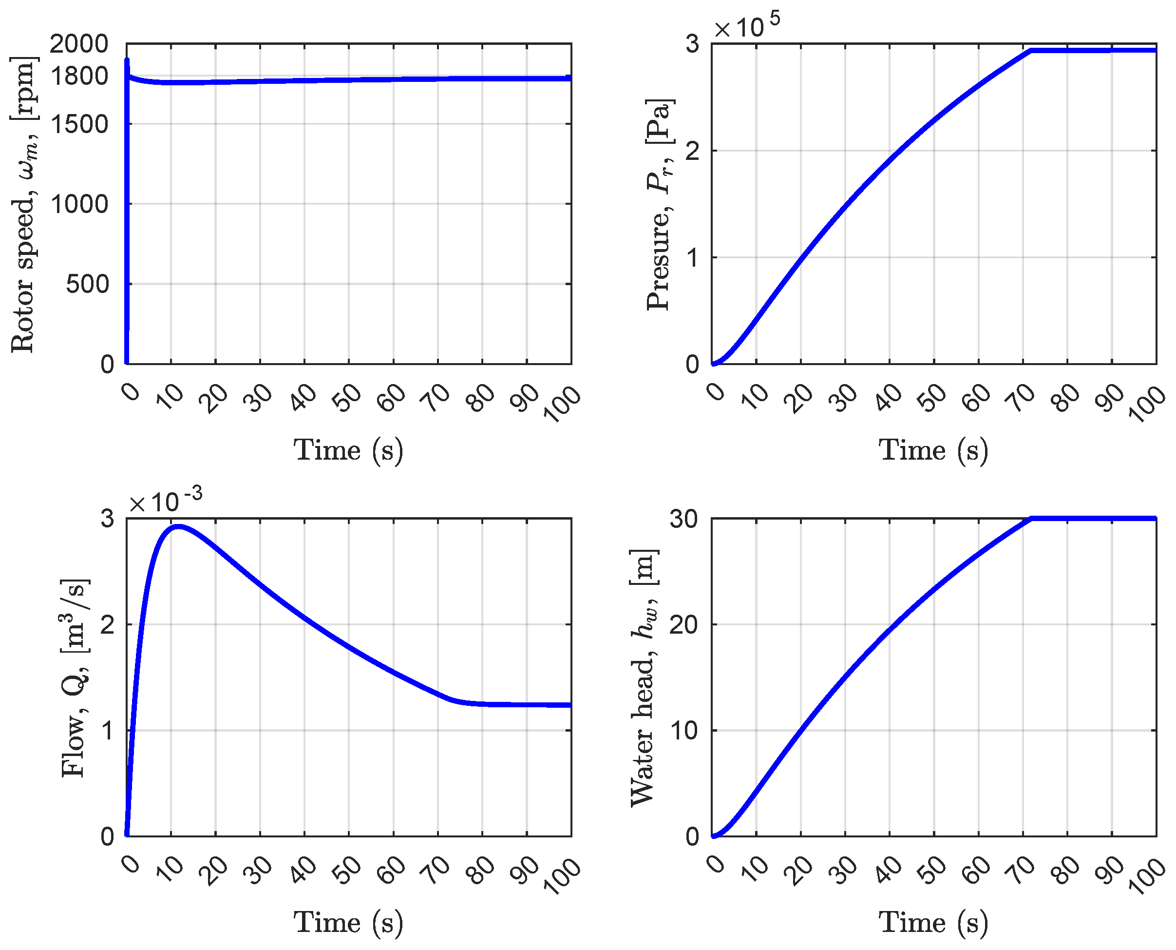
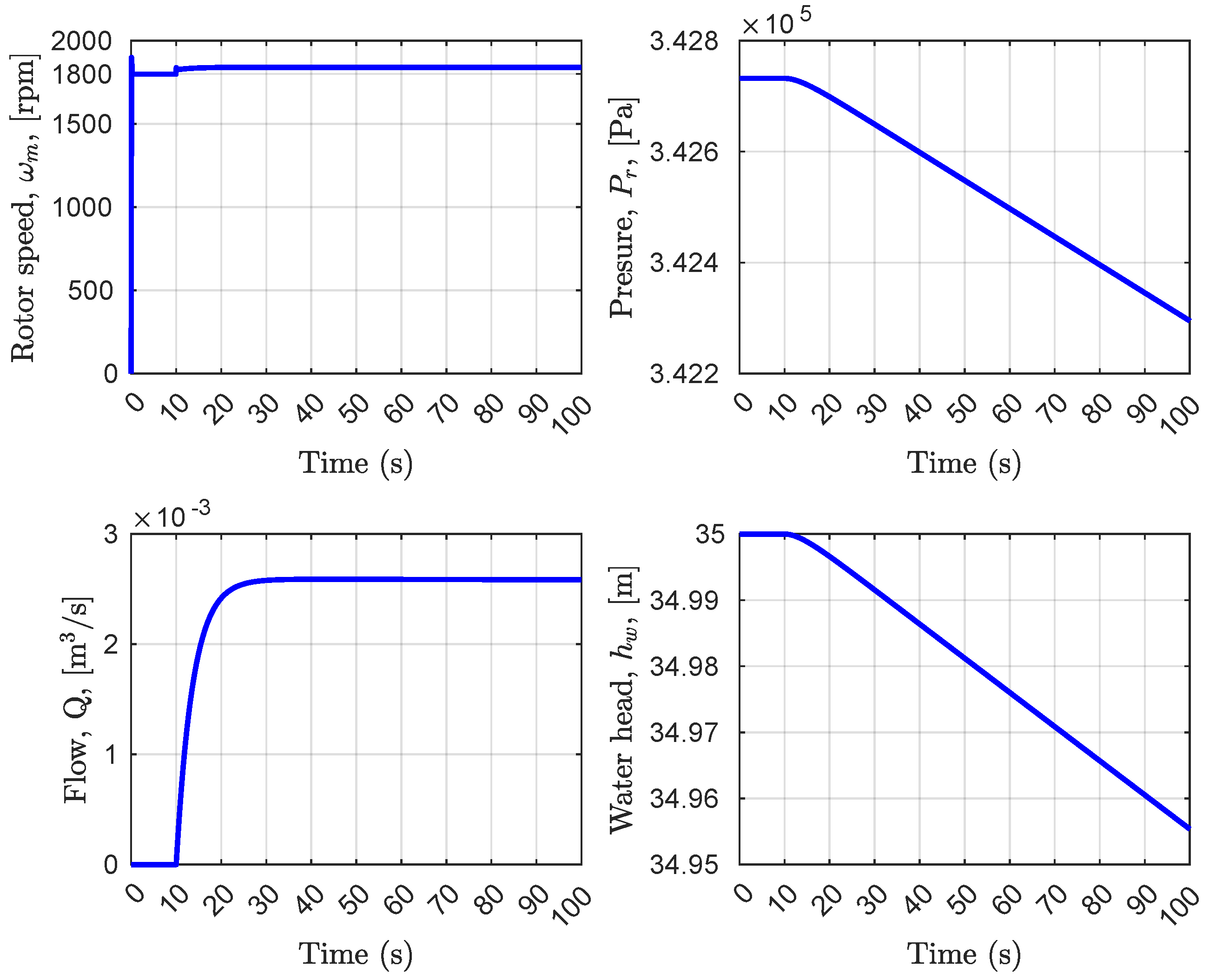
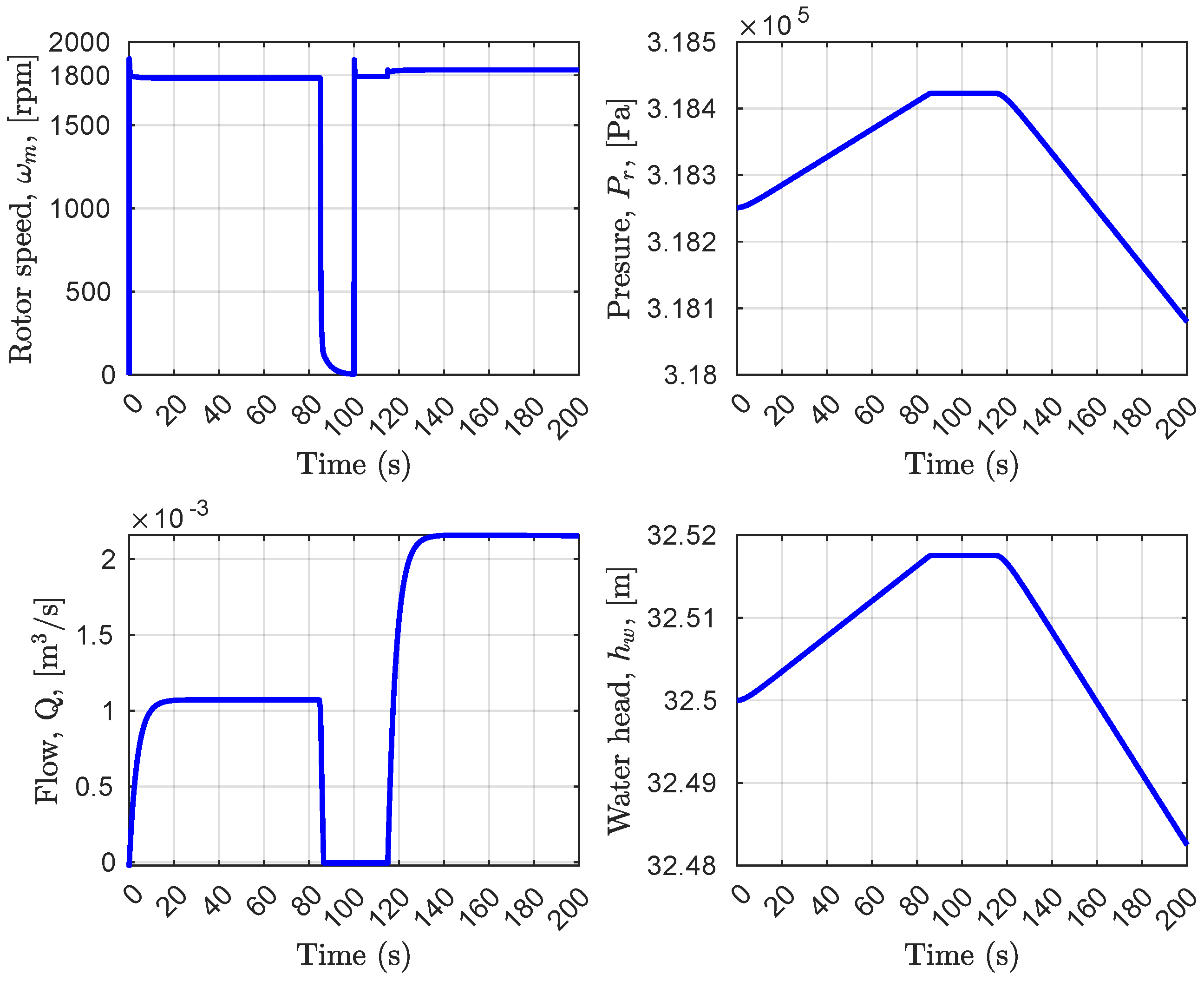
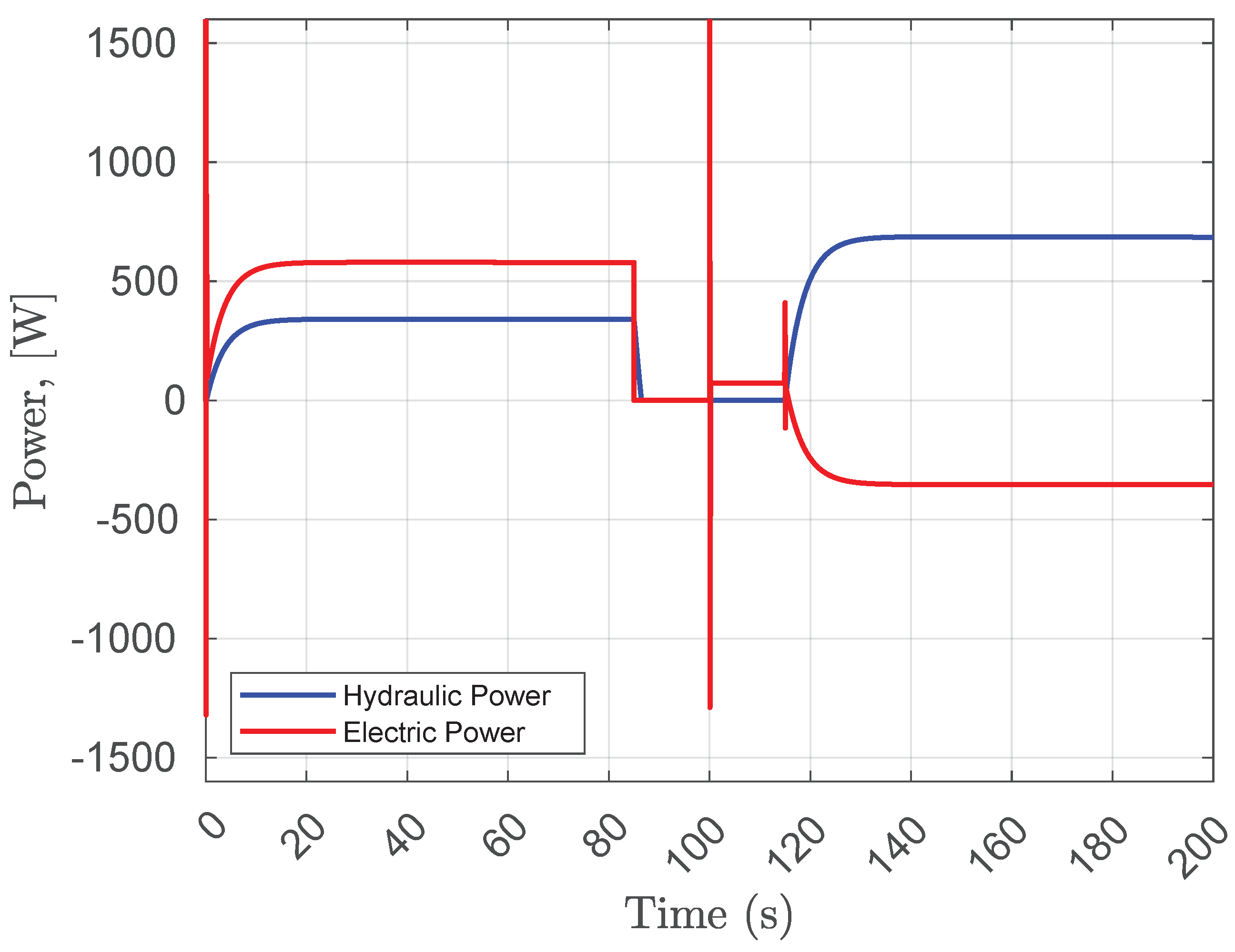
4. Results of Simulations

The system presented in this paper has been simulated in order to obtain validation data. Table 1 shows the main parameters for pump-turbine components. The initial conditions are as follows.

$$\mathrm{col}\left({\lambda }_{s_d},{\lambda }_{s_q},{\lambda }_{r_d},{\lambda }_{r_q},p_{M-P}\right)=\mathrm{col}\left(0,0,0,0,0\right).$$

(48)

We have chosen three different scenarios where the initial conditions for the pressure $P_r\left(0\right)$ and flow $Q\left(0\right)$ are defined accordingly. Furthermore, we assume that $Q\ge 0$ and ${\omega }_m\ge 0$ for all scenarios even though the direction (sign) changes in a real system for the pump or the turbine mode.

First, the system is operated as a hydropump system, i.e., $s=0$ in (45). The initial conditions for the flow and the water height are $Q\left(0\right)=0.0\left({\mathrm{m}}^3/\mathrm{s}\right)$, $P_r\left(0\right)=0.0\left(\mathrm{Pa}\right)$, and $h_w=0.0\left(\mathrm{m}\right)$. Figure 3 shows the resulting dynamics of rotor speed ${\omega }_m$, hydraulic flow Q, hydraulic pressure $P_r$, and water height $h_w$ in the penstock and the reservoir. The water increases its pressure and height in the pipeline at $t\le 70\left[\mathrm{s}\right]$. Then, the reservoir begins to be filled at $t>70\left[\mathrm{s}\right]$ and due to the cross-section area; i.e., $A_r\gg A_p$ (see Table 1) both $P_r$ and $h_w$ have a lower increasing rate. We finally see in the first scenario how the hydraulic flow grows faster during the first seconds, and later on, such an acceleration rate decreases $\left(12<t<75\right)\left(\mathrm{s}\right)$ due to the impulse pressure and the accumulated pressure in the system.

The second scenario simulates the hydroturbine system, i.e., $s=1$ in (45). The simulation results are shown in Figure 4. The initial conditions for the simulation are $Q\left(0\right)=0.0\left({\mathrm{m}}^3/\mathrm{s}\right)$, $P_r\left(0\right)=3.4275\times {10}^5\left(\mathrm{Pa}\right)$, and $h_w=35\left(\mathrm{m}\right)$, which means that the upper reservoir is full of water. The asynchronous machine starts its operation as a motor in $0\le t<10\left(\mathrm{s}\right)$. Then, valve ${\nu }_h$ is opened such that the hydro turbine system is engaged at $t\ge 10\left[\mathrm{s}\right]$. The rotor speed increases above the synchronous speed, which means that the asynchronous machine delivers electricity to the power grid (Figure 1). In Figure 5, we see how the hydraulic flow reaches a stable value while the pressure in the upper reservoir decreases together with the water head of the system.

Finally, the operation of the reversible hydropump–turbine system corresponds to the third simulated scenario. The simulation results are shown in Figure 5. The initial conditions are $Q\left(0\right)=0.0\left({\mathrm{m}}^3/\mathrm{s}\right)$, $P_r\left(0\right)=3.1825\times {10}^5\left(\mathrm{Pa}\right)$, and $h_w=32.5\left(\mathrm{m}\right)$. The system operates first as a hydropump system at $t\le 10\left(\mathrm{s}\right)$ when the asynchronous machine configured as a motor is powered by the electrical network. The water level rises with the pressure in the upper reservoir, which is initially half-loaded. Then, the pumping action is switched off, and the hydraulic valve ${\nu }_h$ in the penstock is closed at $t=85\left(\mathrm{s}\right)$. Both actions co-occur. Similarly to the second scenario, the asynchronous machine starts its operation as a motor in $100\le t<115\left(\mathrm{s}\right)$. The hydraulic valve ${\nu }_h$ opens at $t=115\left(\mathrm{s}\right)$. It follows that the hydroturbine system configuration begins it operation at $t=115\left(\mathrm{s}\right)$. The action over the hydro pump as a turbine system increases the velocity of the rotor ${\omega }_m$ above the synchronous speed, creating a negative slip in the motor that induces a reverse current in the asynchronous machine’s stator. Consequently, the machine ultimately powers the electrical network since it is configured as a generator. It is commonly known that the electrical network regulates the voltage and frequency of the induction generators, which means that a bank of capacitors is unnecessary.

We also show the electrical and hydraulic power generation for the third scenario in Figure 6. As expected, the electrical power is more significant than the hydraulic power for the hydropump system’s operation. During the hydroturbine system’s operation, the opposite occurs, meaning that the hydraulic power is greater than the electric power. The differences in magnitude between electrical and hydraulic power are due to dissipating elements in the system. The change in direction of the electrical power is because it is generated by power and delivered to the grid. Finally, notice the peaks of power at $t=\left(0,100\right)\left(\mathrm{s}\right)$ produced by the start of the asynchronous machine configured as a motor similar to the second scenario.

5. Conclusions

A PH approach to the reversible hydro pump-turbine system has been presented, which is meant to store energy and generate electrical power depending on the user’s desired application. It is clear how the multi-domain characteristic of our model allows a clear interpretation of energy (and power) flow and dissipation thanks to the energy-based approach. The system is reversible thanks to a switch that allows the operation mode to change. The switch naturally falls into the interconnection matrix of the PH modelling approach. Our numerical simulations have confirmed the system’s operation for both modes: pump and turbine. It is clear how the system’s internal energy is contained in the Hamiltonian function. Such Hamiltonian could be shaped with control strategies in order to reach a desired operating point. Then, the new operation point could be attained with key control strategies. For future work, a physical implementation is key in order to validate our model and to test its operation in a real-life system. These validation tests will be performed on a hydraulic and electromechanical test bench that is being prepared for implementation at the time of writing this manuscript. Furthermore, our long-term research objective is to design and implement passivity-based and trajectory-tracking control strategies. Such a closed-loop system would exploit the PH structure for the reversible pump-turbine system. The control objectives will be focused on the power point tracking of the efficiency curves of the asynchronous machine and the centrifugal pump.

References

1. Rehman, S.; Al-Hadhrami, L.M.; Alam, M.M. Pumped hydro energy storage system: A technological review. Renew. Sustain. Energy Rev. 2015, 44, 586–598. [Google Scholar] [CrossRef]
2. Cavazzini, G.; Houdeline, J.B.; Pavesi, G.; Teller, O.; Ardizzon, G. Unstable behaviour of pump-turbines and its effects on power regulation capacity of pumped-hydro energy storage plants. Renew. Sustain. Energy Rev. 2018, 94, 399–409. [Google Scholar] [CrossRef]
3. Jain, S.V.; Patel, R.N. Investigations on pump running in turbine mode: A review of the state-of-the-art. Renew. Sustain. Energy Rev. 2014, 30, 841–868. [Google Scholar] [CrossRef]
4. Shankar, V.K.A.; Umashankar, S.; Paramasivam, S.; Hanigovszki, N. A comprehensive review on energy efficiency enhancement initiatives in centrifugal pumping system. Appl. Energy 2016, 181, 495–513. [Google Scholar] [CrossRef]
5. Betka, A.; Moussi, A. Performance optimization of a photovoltaic induction motor pumping system. Renew. Energy 2004, 29, 2167–2181. [Google Scholar] [CrossRef]
6. Goppelt, F.; Hieninger, T.; Schmidt-Vollus, R. Modeling Centrifugal Pump Systems from a System-Theoretical Point of View. In Proceedings of the 2018 18th International Conference on Mechatronics—Mechatronika (ME), Brno, Czech Republic, 5–7 December 2018; pp. 1–8. [Google Scholar]
7. Wang, L.; Zhang, K.; Zhao, W. Nonlinear Modeling of Dynamic Characteristics of Pump-Turbine. Energies 2022, 15, 297. [Google Scholar] [CrossRef]
8. Zhang, N.; Xue, X.; Sun, N.; Gu, Y.; Jiang, W.; Li, C. Nonlinear Modeling and Stability of a Doubly-Fed Variable Speed Pumped Storage Power Station with Surge Tank Considering Nonlinear Pump Turbine Characteristics. Energies 2022, 15, 4131. [Google Scholar] [CrossRef]
9. Guo, W.; Zhu, D. Nonlinear modeling and operation stability of variable speed pumped storage power station. Energy Sci. Eng. 2021, 9, 1703–1718. [Google Scholar] [CrossRef]
10. Mennemann, J.F.; Marko, L.; Schmidt, J.; Kemmetmüller, W.; Kugi, A. Nonlinear model predictive control of a variable-speed pumped-storage power plant. IEEE Trans. Control Syst. Technol. 2019, 29, 645–660. [Google Scholar] [CrossRef]
11. Perryman, R.; Taylor, J.A.; Karney, B. Port-Hamiltonian Based Control of Water Distribution Networks. Available online: https://papers.ssrn.com/sol3/papers.cfm?abstract_id=4097576 (accessed on 10 June 2022).
12. Li, H.; Chen, D.; Tolo, S.; Xu, B.; Patelli, E. Hamiltonian Formulation and Analysis for Transient Dynamics of Multi-Unit Hydropower System. J. Comput. Nonlinear Dyn. 2018, 13, 101004. [Google Scholar] [CrossRef]
13. Gil-González, W.J.; Garces, A.; Fosso, O.B.; Escobar-Mejía, A. Passivity-Based Control of Power Systems Considering Hydro-Turbine with Surge Tank. IEEE Trans. Power Syst. 2020, 35, 2002–2011. [Google Scholar] [CrossRef]
14. Phillips-Brenes, H.; Pereira-Arroyo, R.; Muñoz-Arias, M. Energy-based model of a solar-powered pumped-hydro storage system. In Proceedings of the 2019 IEEE 39th Central America and Panama Convention (CONCAPAN XXXIX), Guatemala City, Guatemala, 20–22 November 2019. [Google Scholar]
15. Gonzalez, H.; Duarte-Mermoud, M.A.; Pelissier, I.; Travieso-Torres, J.C.; Ortega, R. A novel induction motor control scheme using IDA-PBC. J. Control Theory Appl. 2008, 6, 59–68. [Google Scholar]
16. Yu, H.; Yu, J.; Liu, J.; Song, Q. Nonlinear control of induction motors based on state error PCH and energy-shaping principle. Nonlinear Dyn. 2013, 72, 49–59. [Google Scholar] [CrossRef]
17. Esquivel-Sancho, L.; Pereira-Arroyo, R.; Muñoz Arias, M. An energy-based modeling approach to the induction machine. In Proceedings of the 2021 European Control Conference (ECC), Delft, The Netherlands, 29 June–2 July 2021. [Google Scholar]
18. Esquivel-Sancho, L.; Pereira-Arroyo, R.; Muñoz Arias, M. Voltage regulation for a self-excited induction generator. In Proceedings of the 2021 60th IEEE Conference on Decision and Control (CDC), Austin, TX, USA, 14–17 December 2021. [Google Scholar]
19. Maschke, B.M.; van der Schaft, A.J. Port-controlled Hamiltonian systems: Modelling origins and systemtheoretic properties. IFAC Proc. Vol. 1992, 25, 359–365. [Google Scholar] [CrossRef]
20. van der Schaft, A. L2-Gain and Passivity Techniques in Nonlinear Control; Springer: London, UK, 2000. [Google Scholar]
21. Brogliato, B.; Lozano, R.; Maschke, B.; Egeland, O. Dissipative systems analysis and control. Theory Appl. 2007, 2, 2–5. [Google Scholar]
22. Chan-Zheng, C.; Muñoz-Arias, M.; Scherpen, J.M. Tuning rules for passivity-based integral control for a class of mechanical systems. IEEE Control Syst. Lett. 2022, 7, 37–42. [Google Scholar] [CrossRef]
23. Lee, R.; Pillay, P.; Harley, R. D, Q reference frames for the simulation of induction motors. Electr. Power Syst. Res. 1984, 8, 15–26. [Google Scholar] [CrossRef]
24. Bimal, K. Modern Power Electronics and AC Drives; Prentice Hall PTR: Hoboken, NJ, USA, 2003. [Google Scholar]
25. Stanley, H.C. An analysis of the induction machine. Electr. Eng. 1938, 57, 751–757. [Google Scholar] [CrossRef]
Figure 1. General diagram of reversible hydropump–turbine system.
Applsci 12 09086 g001
Figure 2. In the reference frame of a synchronously rotating asynchronous machine, we can represent the two phases d-q via an equivalent circuit.
Applsci 12 09086 g002
Figure 3. First scenario: operation of the hydro pump system, i.e., s = 0 . The initial conditions are Q 0 = 0.0 ( m 3 / s ) , P r 0 = 0.0 Pa , and h w = 0.0 m , which is the minimum capacity of the penstock and the upper reservoir system.
Applsci 12 09086 g003
Figure 4. Second scenario: operation of the hydro turbine system, i.e., s = 1 . The initial conditions are Q 0 = 0.0 ( m 3 / s ) , P r 0 = 3.4275 × 10 5 Pa , and h w = 35 m , which is the maximum capacity of the penstock and the upper reservoir system.
Applsci 12 09086 g004
Figure 5. Third scenario: operation of the reversible hydropump–turbine system with s = 0 at t 85 s , and s = 1 at t 100 s . Both hydraulic and electromechanical systems are switched off between 85 < t < 100 s . The asynchronous machine and the hydraulic system are switched on at t = 100 s and t = 115 s , respectively. The initial conditions are Q 0 = 0.0 ( m 3 / s ) , P r 0 = 3.1825 × 10 5 Pa , and h w = 32.5 m .
Applsci 12 09086 g005
Figure 6. Power transformation of third scenario: The system works in pumping mode at t 85 s taking energy from the electric network, which is converted into mechanical (hydraulic) energy. Both hydraulic and electromechanical systems are switched off between 85 < t < 100 s . At t = 100 s , the asynchronous machine is switched on again in the motor mode, taking energy from the electric network. Then, at t = 115 s , the hydraulic system is also switched on, inducing the system to start its operation in the generator-turbine mode. Subsequently, mechanical energy is converted into electrical energy, which is supplied to the power grid. The initial conditions are Q 0 = 0.0 ( m 3 / s ) , P r 0 = 3.1825 × 10 5 Pa , and h w = 32.5 m .
Applsci 12 09086 g006