
Ship Shaft Frequency Extraction Based on Improved Stacked Sparse Denoising Auto-Encoder Network
1
Shanghai Acoustics Laboratory, Institute of Acoustics, Chinese Academy of Sciences, Shanghai 201815, China
2
University of Chinese Academy of Sciences, Beijing 100049, China
*
Author to whom correspondence should be addressed.
Appl. Sci. 2022, 12(18), 9076; https://doi.org/10.3390/app12189076
Submission received: 21 July 2022
/
Revised: 6 September 2022
/
Accepted: 8 September 2022
/
Published: 9 September 2022
(This article belongs to the Special Issue Underwater Acoustic Signal Processing)
Abstract
:The modulation spectrum of ship radiated noise contains information on shaft frequency, which is an important feature used to identify ships and a key parameter involved in calculating the number of propeller blades. To improve the shaft frequency extraction accuracy, a ship shaft frequency extraction method based on an improved stacked sparse denoising auto-encoder network (SSDAE) is proposed. Firstly, the mathematical model of the ship radiated noise modulation spectrum is built and data simulation is carried out based on this model, combined with the actual ship parameters. Secondly, we trained the SSDAE model using the simulation data and made slight adjustments to this model by using both simulation and measured data to improve it. Finally, the experimental ship modulation spectrum information was input to the SSDAE model for denoising, enhancement, and regression estimation. Accordingly, the shaft frequency was extracted. The simulation and experimental results show that the shaft frequency extraction method based on the improved SSDAE model has high accuracy and good robustness, especially under the conditions of both missing line spectra and noise interference.
1. Introduction
In the process of a ship’s movement, propeller blades cut the water flow, creating ship radiated noise with a periodic fluctuation envelope, which is audibly expressed as a rhythmic time-varying loudness characteristic [1]. Therefore, the envelope spectrum of ship radiated noise carries information such as shaft frequency and propeller number [2], which can be used for ship identification with high robustness. In practical applications, the accurate extraction of shaft frequency is a key step in calculating the number of propeller blades, which plays an important role in the field of passive sonar target recognition.
At present, researchers have carried out much work concerning shaft frequency feature extraction and have achieved considerable results in mathematical modeling [3,4,5]. These studies reveal the physical mechanism of the modulation phenomenon of ship radiated noise, and provide a mathematical basis for the simulation of ship modulation spectrum data. In terms of shaft frequency extraction, a maximum likelihood estimation method of propeller speed is proposed in [6], and a closed-loop detection method for shaft frequency in propeller noise is proposed in [7]. In the work of [8], the application of a Duffing oscillator in extracting line spectrum of weak amplitude demodulation of ship radiated noise is studied. In the work of [9], a new method of envelope line spectrum denoising based on complementary integrated empirical mode decomposition (CEEMD) and wavelet threshold is investigated. The auditory spectrum extraction technology is improved to obtain a significant envelope spectrum at a low signal-to-noise ratio in the work of [10]. In the work of [11], a method for extracting the frequency characteristics of the ship radiated noise envelope using a dual frequency method is proposed. The propeller shaft frequency feature extraction algorithm for underwater acoustic targets based on the average energy accumulation and pulse sequence matching is proposed in [12]. These methods determine the value of shaft frequency by looking for harmonic line spectrum clusters generated by propeller blade modulation, which is better for shaft frequency extraction of high-quality modulation spectra. However, due to the shaft imbalance of propeller blade assembly, the envelope spectrum of ship radiated noise usually has different degrees of missing line spectra [5]. In addition, the envelope spectrum tends to have a low signal-to-noise ratio and is prone to non-harmonic line spectra due to the interference of environmental and other ship radiated noise [13]. These questions are not widely appreciated in existing studies and are the factors that cause inaccuracy with respect to shaft frequency extraction by traditional methods.
Deep learning has achieved remarkable results in the fields of speech recognition and computer vision. In recent years, deep learning models such as deep neural networks, auto-encoder networks, and convolutional neural networks have been widely used for line spectrum enhancement and target recognition of ship radiated noise [14,15,16,17,18,19]. Deep learning can fit the complex mapping relationship from input to output through data learning to achieve tasks of target classification and regression prediction [20,21]. It has a powerful nonlinear modeling ability and is an effective means to deal with nonlinear problems in ship shaft frequency extraction.
To improve the accuracy of shaft frequency extraction in the case of a missing line spectrum and low signal-to-noise ratio, a ship shaft frequency extraction method based on improved SSDAE is proposed in this paper. In this method, SSDAE is used to enhance the propeller shaft frequency line spectrum and its harmonic line spectrum, and the depth regression network is used to accurately estimate the ship shaft frequency. Experimental results show that the robustness and the accuracy of shaft frequency extraction are improved in the above cases. Additionally, this method has better stability under different spindle speeds and has obvious advantages over the traditional algorithm in computing speed. It has high practical application value in the target recognition system of the passive sonar platform.
The remainder of this paper is organized as follows. In Section 2, we build the mathematical model of ship radiation noise modulation spectrum. In Section 3, we propose the improved SSDAE network model. The training and fine-tuning methods for improved SSDAE are presented in Section 4. Experiment and result analysis of shaft frequency extraction are demonstrated in Section 5. The conclusions of this work are highlighted in Section 6.
2. Mathematical Model of Ship Radiation Noise Modulation Spectrum
The ship radiated noise signal obtained by the passive sonar system can be approximated as
where is the ship radiated noise signal, is the propeller noise with envelope modulation characteristics, and is the non-modulated component of the propeller noise as well as the radiated noise and environmental noise of other vibration systems of the ship. The signal-to-noise ratio can be defined as:
For a ship with the M-blade propeller, one cycle in its propeller noise time-domain signal consists of M pulses, so it is divided into a group.
The modulated signal envelope is assumed to be modeled as an impulsive stochastic process with a grouped structure, the same shape, the same repetition period, and a random amplitude [22,23]. For a ship with the m-blade propeller, one cycle of propeller noise time-domain signal includes M pulses, so it is divided into a group. Assuming that the shaft frequency period of the ship is T, the pulse repetition period is T/M. The envelope function consisting of 2N + 1 groups of pulses can be expressed as
where is the amplitude of the mth pulse of the nth group, and is the expression of the pulse waveform. Assuming that the single pulse waveform is Gaussian [24,25], can be expressed as
where is a parameter that affects the pulse width. is a mutually independent random variable subject to a certain probability distribution. In the specific calculation, take the average value of the amplitude , and satisfies
The propeller noise is a kind of cavitation noise, which is mainly generated by the propeller blades periodically cutting water resulting in the fragmentation of bubble groups. The signal is a non-stationary process [26], which can be regarded as the product of envelope modulation signal and stationary signal, which is
In the simulation of ship radiated noise, the bubble cluster noise is approximated as Gaussian noise [27]. The power spectrum analysis (Fourier transform) of propeller cavitation noise signal is performed with
where , is the sampling frequency, N is the number of sampling points of a signal. Approximating the modulation spectrum of the ship radiated noise as the power spectral density of the propeller noise signal, then
The modulation spectrum of ship radiation noise consists of a line spectrum and a continuous spectrum [28], which is different from the power spectrum in that the line spectrum in the modulation spectrum has the harmonic relationship and group structure, in which the frequency corresponds to the fundamental line spectrum is the ship shaft frequency.
3. SSDAE-DRN Network
3.1. Theory of SSDAE
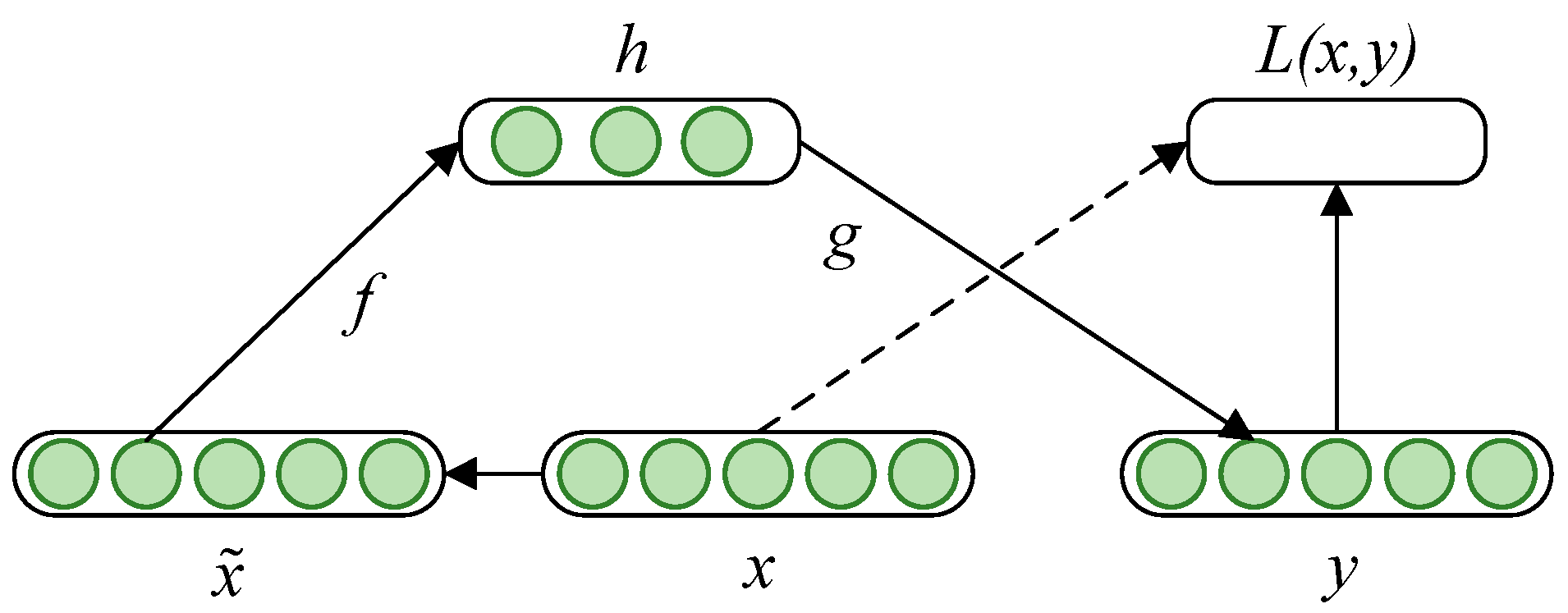
A denoising auto-encoder [29] (DAE) is a three-layer neural network consisting of an input layer, a hidden layer, and an output layer, and the flow of the DAE algorithm is shown in Figure 1. After adding noise to the original input x, the interference input is obtained, and the input feature expression h is obtained through the encoding function fθ. Then h is mapped to the output layer through the decoding function gθ to obtain the reconstructed data z of the input data.
Therefore, the encoding process of DAE can be expressed as
where θ = (w,b) is the coding model parameter; w is the coding weight matrix, and b is the coding offset vector. The decoding process can be expressed as
where is the decoding model parameter, is the decoding weight matrix, is the decoding offset vector, and is the nonlinear activation function. The reconstruction result z cannot accurately reproduce the input data x, for the training sample set , the cost function of DAE is
where is is the weight, and the over-fitting can be reduced by decreasing the weight. In addition, a penalty factor is added to the cost function to limit the activation degree of the neurons in the overall hidden layer, which can realize the high-dimensional sparse feature extraction of the input data. Therefore, the cost function of the sparse denoising auto-encoder (SDAE) is
where is the sparsity parameter, is the weight of the control sparse constraint, and is the average activation of the input data corresponding to the jth node of the hidden layer [30].
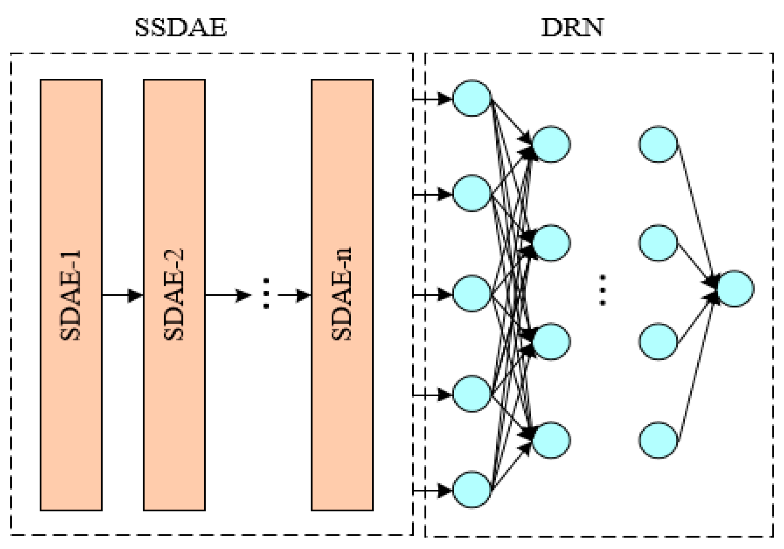
SSDAE is a deep neural network formed by stacking several SDAE, and the output vector of the previous SDAE hidden layer is the input vector of the next SDAE. The training of SSDAE adopts the greedy layer-by-layer training method that can effectively alleviate the gradient dispersion phenomenon [31]; that is, each SDAE is trained separately to obtain the optimal weight of the network which is used as the SSDAE network weights. The network is then fine-tuned overall by the error back propagation (BP) algorithm [32] until the optimal parameters of the network are derived. The cost function of the fine-tuning process of SSDAE is
where L is the number of SDAE. There is no sparsity constraint for fine-tuning since the sparsity penalty has been included in the pre-training of each SDAE.
3.2. Improved Method of SSDAE
3.2.1. Establishment of Regression Model
SSDAE is an unsupervised deep neural network, which is usually applied to feature extraction and data denoising, it can be used for target recognition combined with the SoftMax [33] classification algorithm. To realize the extraction of ship shaft frequency, a depth regression network (DRN) is connected after SSDAE. The modulation line spectrum of ship radiated noise is enhanced by SSDAE, and the output vector of SSDAE is used as the input vector of DRN to obtain the regression model based on SSDAE, namely SSDAE-DRN, to realize the feature extraction of modulation line spectrum and the estimation of ship shaft frequency. DRN is a supervised deep learning network with sequence sensitivity [34], which can extract position and structural features of the line spectrum. During the training, the labeled shaft frequency corresponding to the SSDAE denoising modulation spectrum is taken as the output. Then, the features are extracted by the network and the mapping relationship between the modulation spectrum and the shaft frequency is constructed. The weight matrix of DRN is updated by the BP algorithm with the following cost function
The mean absolute error (MAE) is used as an index to measure the accuracy of shaft frequency estimation of the model, the average MAE over N samples is defined as
where denotes the expected value of the output layer node, and represents the actual output value of the output layer node. The improved SSDAE model (SSDAE-DRN) of ship shaft frequency extraction is shown in Figure 2.
3.2.2. Activate Function
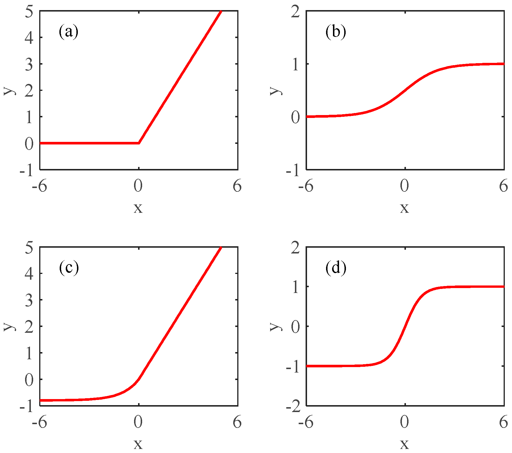
The SSDAE-DRN network trained with different nonlinear activation functions has different feature representation and fitting generalization capabilities, which can affect the accuracy of shaft frequency extraction. We choose the Elu function as the activation function of the hidden layer, and the expression is
Compared with traditional Sigmoid and Tanh functions, the ELU function can overcome the problem of gradient disappearance during iteration [35]. Meanwhile, the ELU function has a non-zero exponential distribution slope on (−∞, 0), which can effectively alleviate the problem of hard saturation of negative input of Relu function. Images of Relu, Sigmoid, ELU, and Tanh activation function are shown in Figure 3. The traditional network output layer is usually activated by SoftMax or Sigmoid function to achieve target classification or numerical prediction. In this paper, we improve the activation function according to the actual needs of ship modulation spectrum denoising and shaft frequency extraction. SSDAE and DRN have actual output range constraints and no negative values for the modulation spectrum so they are activated by the Relu function. The output of DRN is the estimate of the modulation spectrum shaft frequency, so there is no activation function.
3.2.3. Batch Normalization
To extract features better, reduce the dependency between parameters, and alleviate the phenomenon of over-fitting, the nonlinear activation function is used after each layer of weighted summation in the feature extraction network to enhance the nonlinear expression. Meanwhile, in order to accelerate the convergence of the network, prevent gradient explosion, and improve the accuracy of the model, a batch normalization (BN) layer is added before the activation function so that the input will not always be in a negative interval. The calculation of the BN layer can be seen in formula (17).
where is the output of the dense layer, and represent the mean and variance, respectively, is the output of the BN, is the numerical stability constant, and are the optimizable parameters of the BN layer to ensure that the normalization can optimize the distribution of activation values.
4. Training and Fine-Tuning of SSDAE-DRN
It is difficult to obtain the radiated noise of ships, especially the data under different spindle speeds, which limits the training effect and generalization ability of the deep learning algorithm. In Section 1, a mathematical model of ship radiated noise modulation spectrum with arbitrary shaft frequency and blade number based on Gaussian pulse signal is established, which creates conditions for ship modulation spectrum database extension and SSDAE-DRN model training. Based on the analysis of the inherent physical characteristics and the modulation spectrum data of the ship, the modulation signal parameters are summarized (as shown in Table 1).
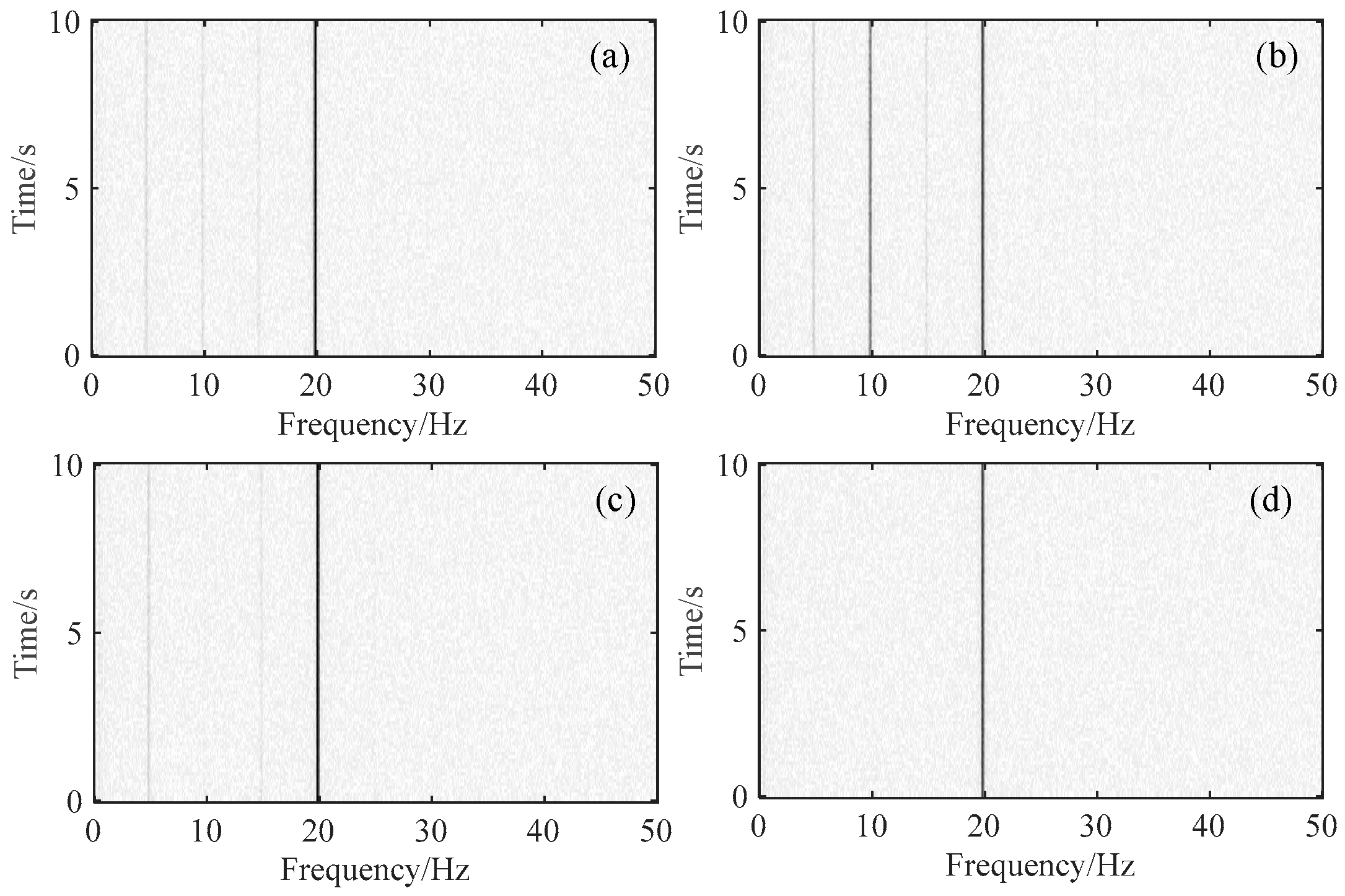
According to the mathematical model of the modulation spectrum and the signal parameters shown in Table 1, the grid search algorithm is used for traversal simulation. The modulation spectrum simulation data is obtained after normalization with shaft frequency as the “label”, and the number of samples is 106. Among them, the simulated modulation spectrum trace of a 4-blade propeller ship with a shaft frequency of 5 Hz under a typical modulation system is shown in Figure 4. In the simulated envelope spectrum of ship radiated noise shown in Figure 4, the line spectrum at 5 Hz is the shaft frequency line spectrum, the line spectrum at 10 Hz is the second harmonic line spectrum, the line spectrum at 15 Hz is the third harmonic line spectrum, and the line spectrum at 20 Hz is the forth harmonic line spectrum. The envelope spectrum shown in the four subplots all have different degrees of line spectrum missing, and in Figure 4 there is only the 4th harmonic line spectrum of the shaft frequency.
According to the difference between blade modulation, the propeller noise envelope modulation can be divided into uniform modulation and non-uniform modulation. In uniform modulation, the modulation system is the same for each blade, and there is only a leaf frequency line spectrum exists in the modulation spectrum, as shown in Figure 4d. In non-uniform modulation, the modulation system of each blade is different, and in some specific cases, there is a lack of line spectrum, as shown in Figure 4c. The absence of a line spectrum will lead to the poor robustness of the shaft frequency extraction algorithm, the existence of only a leaf frequency line spectrum will lead to the misjudgment of the axis frequency. The actual ship modulation spectrum often has line spectrum components lower than shaft frequency, which are important factors to reduce the accuracy of shaft frequency extraction.
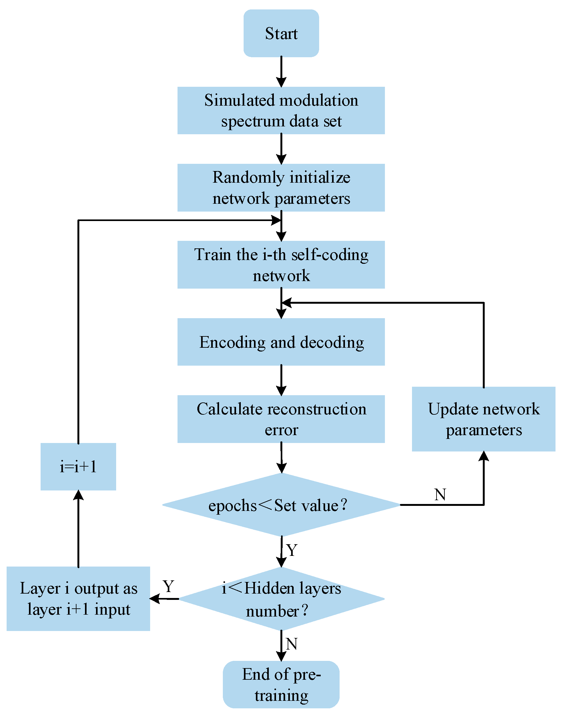
The training of SSDAE is divided into two steps: unsupervised pre-training and supervised fine-tuning. Unsupervised pre-training takes the original simulation data after adding noise as the network input, and adopts a greedy algorithm to train layer-by-layer, so that the network learns to reconstruct the intrinsic features of the original data by minimizing the cost function (as shown in Figure 5).
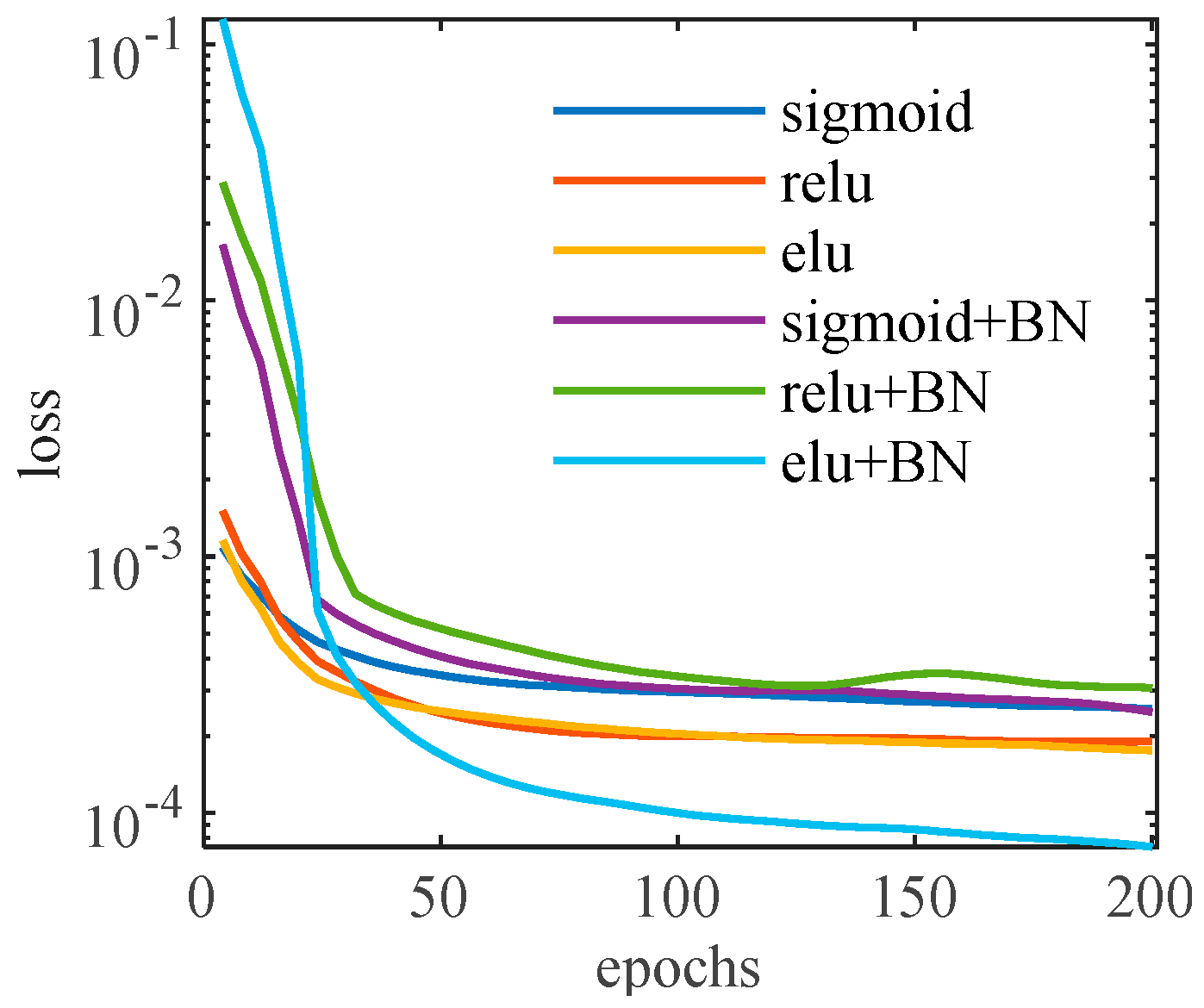
Next, the SSDAE-DRN model is trained according to Figure 5. The number of input layer nodes is 1500 and the number of hidden layers is 6. The Adma optimizer is used to optimize the network parameters, the learning rate is set to 0.001 and the number of iterations is 200. To evaluate the performance of the model and avoid the overlapping of shaft frequency and blade frequency of different data, which makes the model unable to be generalized, data with shaft frequency as an integer and blade number as 7 in the simulation data are used for training. The training and validation sets are divided according to the proportion of 3:2. Experiments are carried out on networks with different activation functions and batch normalization, and the cost function curves are shown in Figure 6.
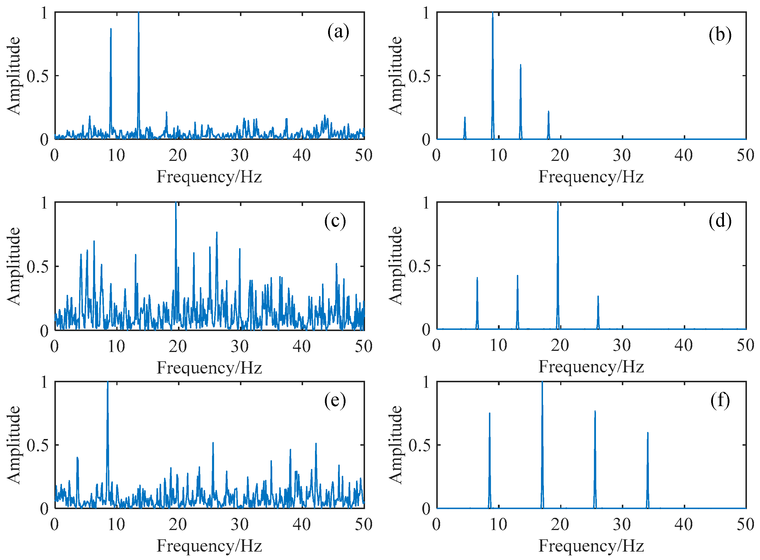
When using ELU function activation and BN layer for batch standardization, the network cost function curve is smoother and the convergence value is smaller, which has better reconstruction performance of the original data. After the model training is completed, the simulated modulation spectrum is input into the pre-trained SSDAE-DRN model, and the reconstructed results are shown in Figure 7.
The shaft frequencies corresponding to the input data shown in Figure 7 are 4.5 Hz, 6.5 Hz, and 8.5 Hz, respectively, and these non-integer shaft frequency samples are not included in the training data. The comparison between the output data and the input data shows that the harmonic line spectrum is significantly enhanced, the continuous spectrum envelope is effectively suppressed, the submerged or missing shaft frequency line spectrum is recovered, and the non-harmonic line spectrum is effectively eliminated.
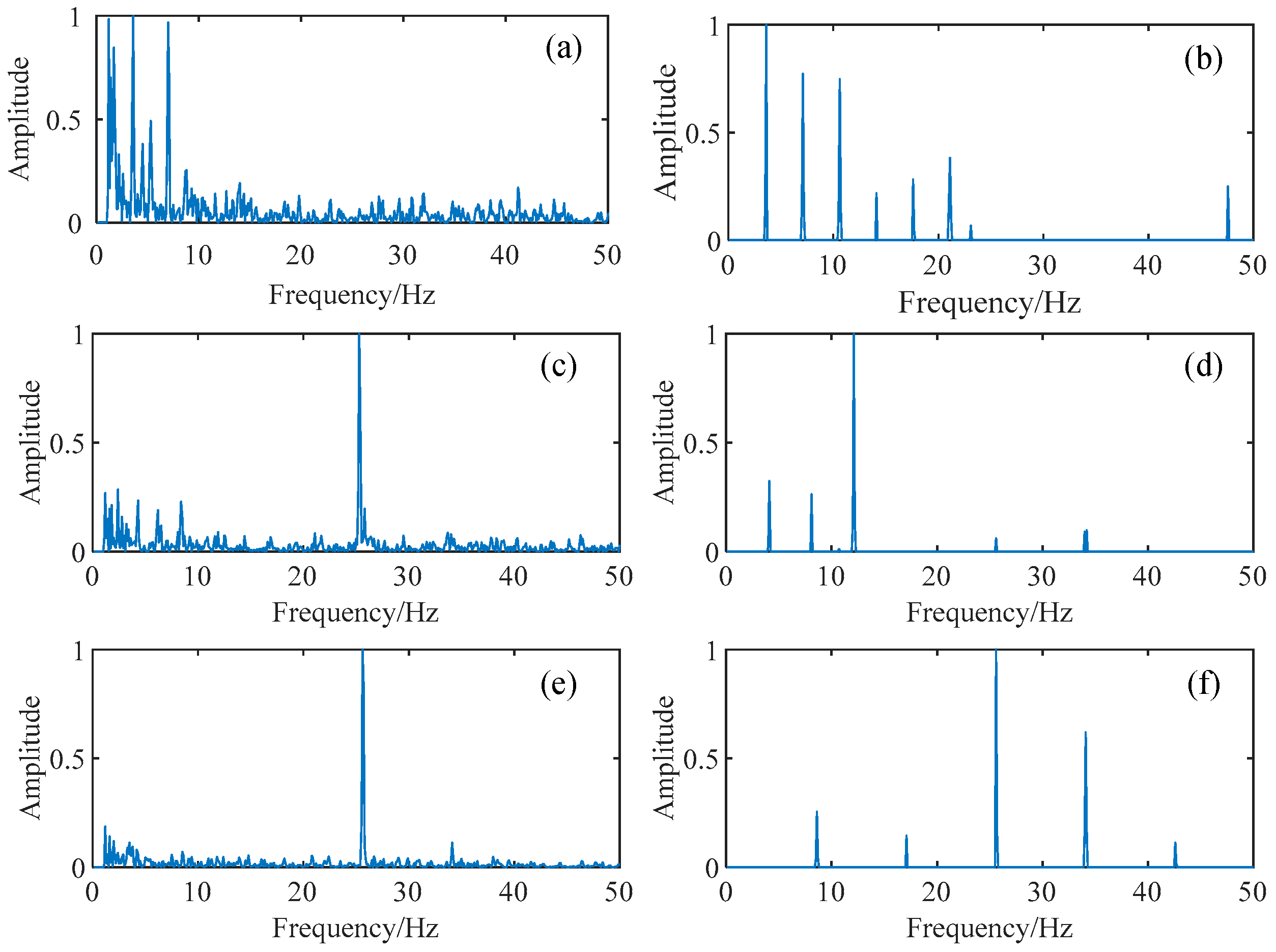
Since the number of effective line spectra of the data used in the training model is 7, the higher harmonic line spectra of the output are inevitably enhanced, but this does not hinder the subsequent task of shaft frequency extraction. Input the modulation spectrum data of the radiated noise of three ships into the model, and the reconstruction results are shown in Figure 8. It can be seen that the SSDAE-DRN model has a good generalization ability and denoising effect on the real data. In particular, Figure 8d,f reflect the ability of the model to accurately restore the axial shaft frequency line spectrum and the harmonic line spectrum between the shaft frequency and the leaf frequency line spectrum, which is based on the leaf frequency line spectrum and the higher harmonics information. This shows that the model possesses the sensitivity of line spectrum components and harmonic relationships and is not affected by the change of position.
Then, the simulation data and some real historical data are mixed to form a new dataset, which is used to fine-tune the regression part of SSDAE-DRN so that the model has the capability of shaft frequency extraction. The real data comes from 2000 samples of two cooperative ships in the Qiandao Lake at different speeds, which enables the model to effectively extract line spectrum features, better learn continuous spectrum envelope features and noise distribution rules, and improve the shaft frequency extraction performance of the network. A total of 1500 real samples are randomly selected to fine-tune the SSDAE-DRN model, and 500 samples are used to test the performance of the model. During fine-tuning, the pre-trained SSDAE model parameters are frozen and will not participate in the adjustment of the regression. The experimental results of the model with different combinations of the dataset are shown in Table 2.
Using simulated data to fine-tune the model, the MAE is validated on the simulated data at 0.58 Hz while it is increased by nearly 1 Hz when validated on the measured data. This is mainly due to the fact that the real data are not used in the training of the SSDAE-DRN model, so the model has limited denoising and enhancement effect on real data. However, the regression part of the SSDAE-DRN model has feature extraction capability. Real data are added to fine-tune the model so that it can effectively learn the reconstruction features and improve the accuracy of shaft frequency extraction. Then the model is fine-tuned with both simulated and real data and validated with real data. The MAE is reduced by 0.33 hz, and the model’s performance is improved.
5. Experiment and Result Analysis of Shaft Frequency Extraction
5.1. Simulated Experiment
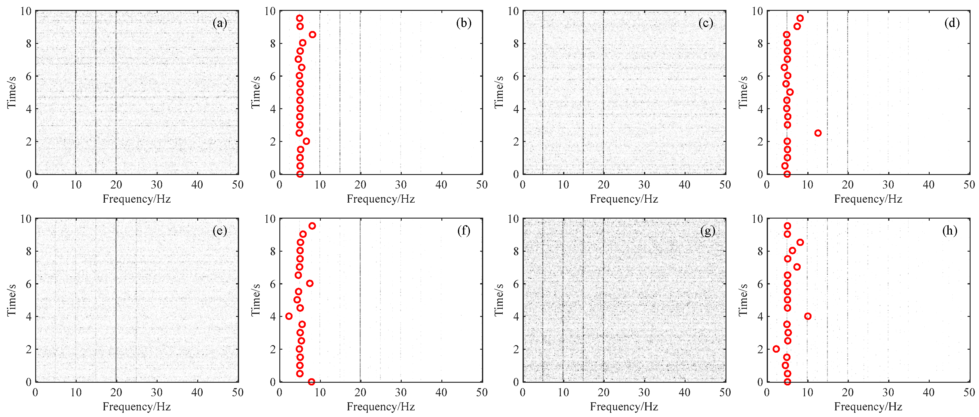
The performance of the SSDAE-DRN model for shaft frequency extraction is tested in the following four cases: shaft frequency line spectrum missing, second harmonic line spectrum missing, strong leaf frequency line spectrum only, and low signal-to-noise ratio. The results of shaft frequency extraction are shown in Figure 9. The left is the trace map of input data, the right shows the output trace map of the denoising and enhancement part of SSDAE-DRN, and the red dots are the estimated shaft frequency of regression prediction. It is worth noting that the input to the SSDAE-DRN model is the envelope spectrum of the ship radiated noise and that the trace map is made up of the envelope spectra stacked in chronological order.
It can be seen from Figure 9 that the SSDAE-DRN model can obtain a more accurate shaft frequency estimation in the case of missing shaft frequency line spectra. The estimation error increases in the other three cases but the shaft frequency can still be extracted more accurately. The method proposed in this paper is compared with the method of sequence matching in [13] on simulated data, and the results are shown in Table 3. Compared with sequence matching, the method in this paper has higher accuracy and obvious advantages, especially in the case of missing line spectra and noise interference.
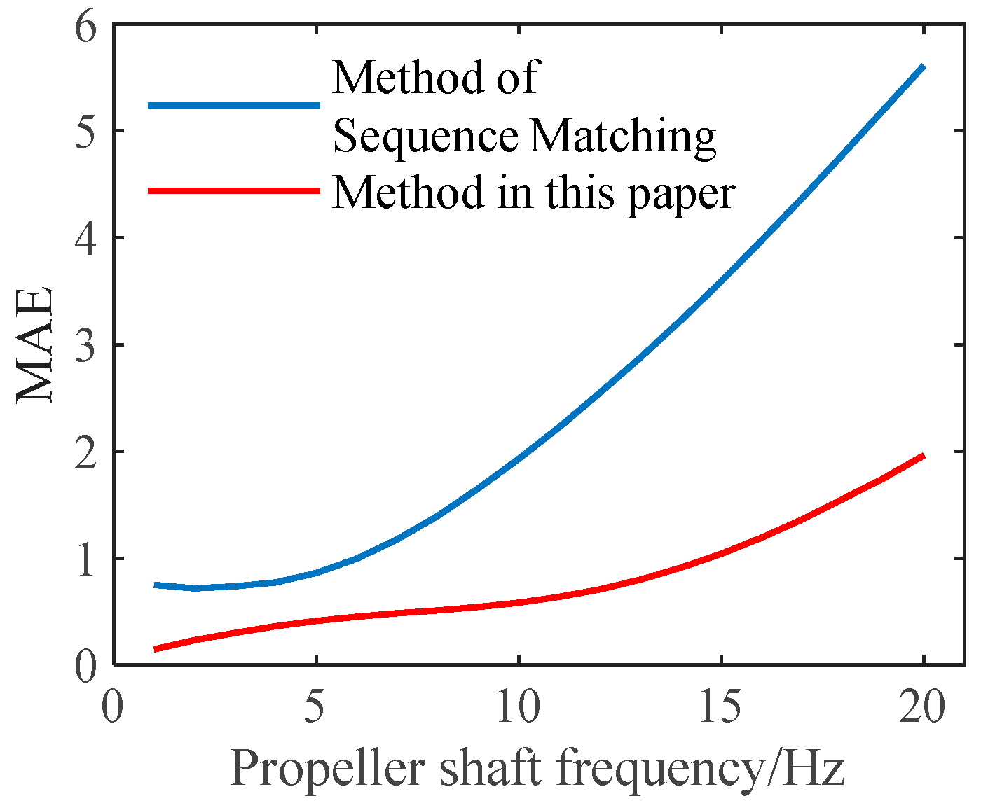
The ship shaft frequency extraction algorithm varies in its ability on different data, and the extraction error increases as the true value increases. To obtain the error distribution of this method, the test data are grouped and the shaft frequency is extracted for each group, respectively. Results obtained by two methods are shown in Figure 10 after smoothing.
Similar to the traditional method, the error of the method in this paper also increases with the increase of the real shaft frequency. Compared with the method of sequence matching, the error growth curve of this method is smoother, and the average absolute error of extraction under the real shaft frequency of 20 Hz is only 2 Hz, which is 3.6 Hz lower than the method of sequence matching. Therefore, the performance of the method in this paper is more stable for ship targets with different speeds.
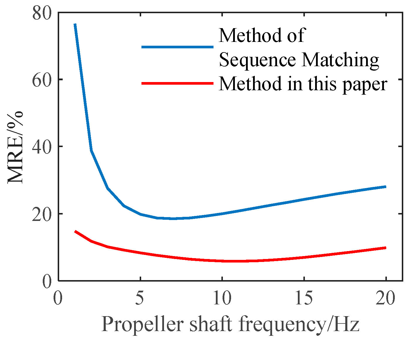
To better measure the performance of the model for shaft frequency extraction at different speeds, the mean error rate is used as the evaluation index, which is defined as
where and are the real and estimated value of the shaft frequency of the nth sample. The distribution of the error rate on the simulated data for the method in this paper and the method of sequence matching is shown in Figure 11.
The shaft frequency line spectrum and harmonic line spectrum in the ship modulation are tight at low speeds, and the interference of the non-harmonic line spectrum makes the traditional method prone to misjudgment. The shaft frequency of the majority of civil ships is no higher than 10 Hz, and usually below 5 Hz during normal driving. Figure 11 illustrates that the method in this paper has a smaller average error rate and significant improvement, especially in the low-speed condition of the ship.
5.2. Experiment on Real Data
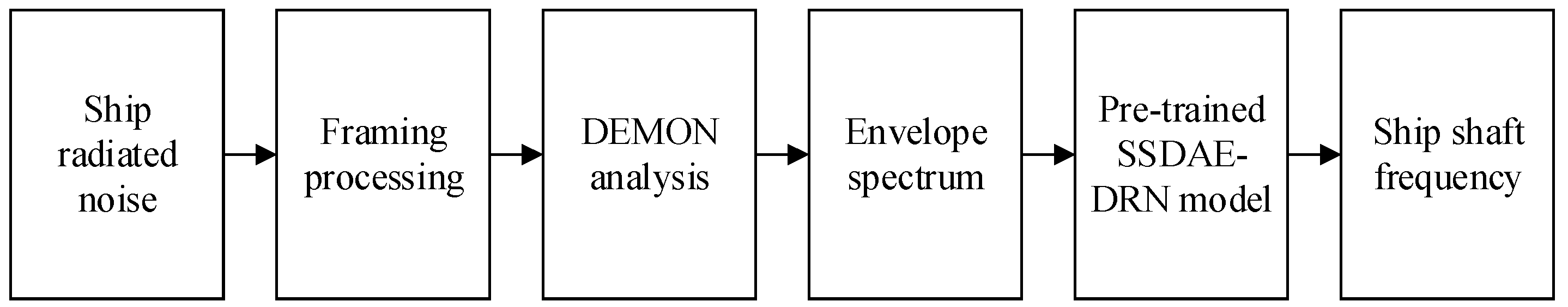
In the simulation experiment, we trained the SSDAE-DRN model by using the simulated ship radiated noise envelope spectrum and a small amount of real ship radiated noise envelope spectrum. Next, we collected the real ship radiated noise data and extracted the ship shaft frequency using the pre-trained SSDAE-DRN model. The main process is shown in Figure 12.
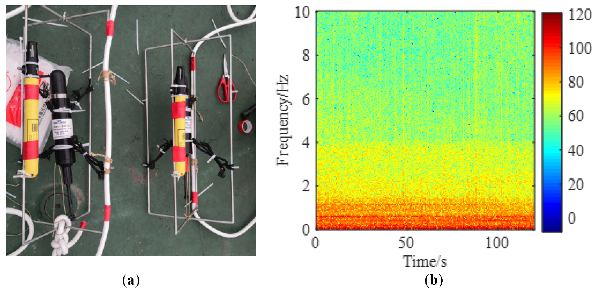
The measurement experiment of ship radiated noise was carried out in a certain area of Changjiang River, in January 2022, where the water depth was 14 m and a large number of cargo ships, tankers, large junks, and law enforcement vessels passed by. The hydrophone is fixed on a frame and placed at a depth of 12 m underwater, at a distance of 750 m from the center of the channel, and the radiated noise is automatically recorded when the ships pass on the river near the hydrophone. The hydrophone used in the experiment is icListen-900 m produced by Ocean Sonics, and the effective measurement frequency band is 0~10 kHz. The experiment equipment and time-frequency diagram of data are shown in Figure 13.
The acquired data are influenced by the sea state and the target distance during the experiment and have the interference of environmental and other ship noise. The radiated noise data of 10 ships in 4 categories are obtained, and the sampling rate is 32 kHz. The ships sail at approximately uniform speed with a shaft frequency range of 2 Hz to 8 Hz. A total of 720 cargo ship samples, 480 tanker samples, 960 large junk samples, and 480 law enforcement vessel samples are obtained after pre-processing.
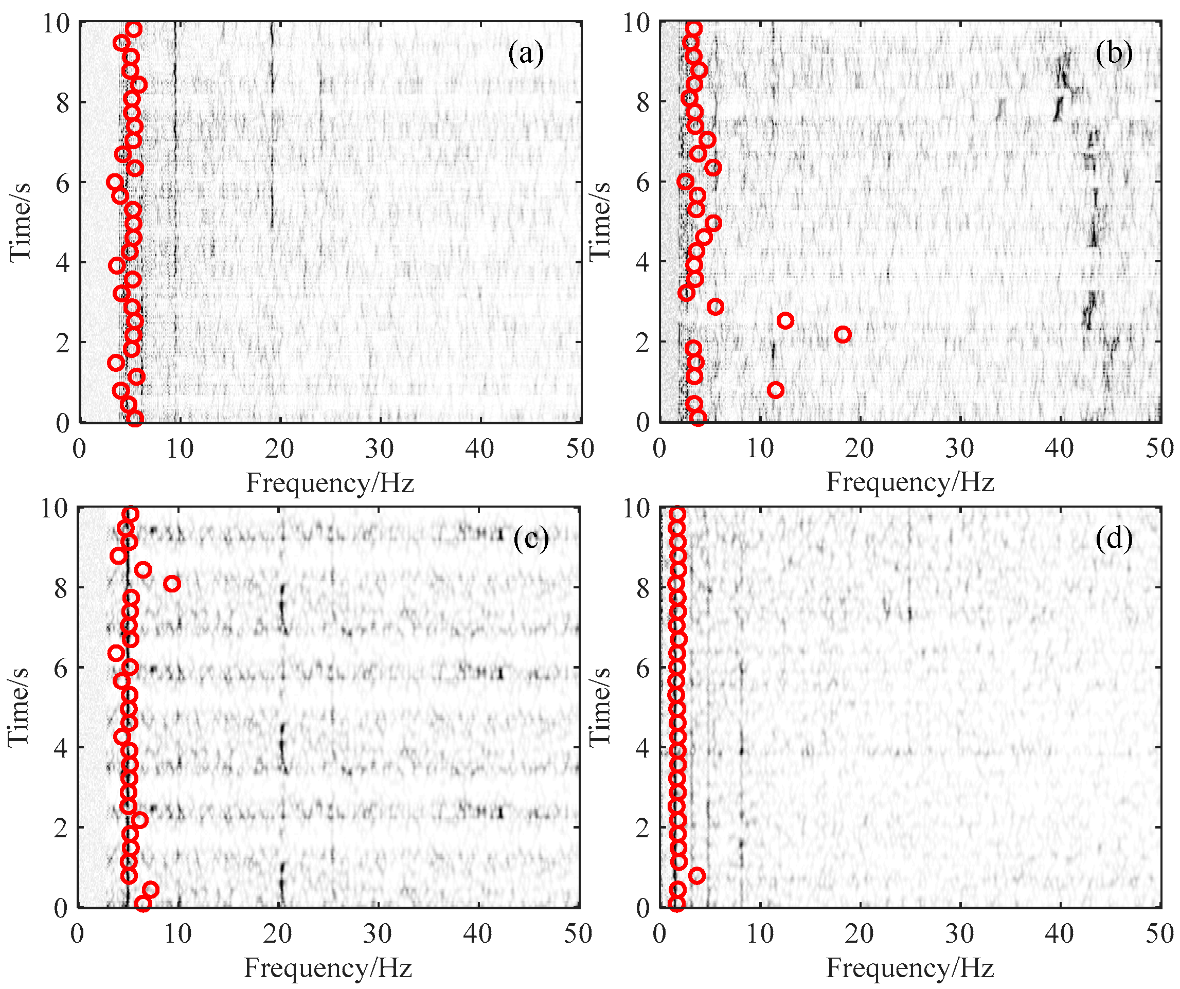
The multi-subband weighted fusion DEMON spectrum estimation method [35] is used to obtain the modulation spectrum of real ship radiated noise, and the real shaft frequency calibration of the sample is then performed by manual interpretation combined with the speed record. The modulation spectrum of the real data is input into the SSDAE-DRN model to obtain the estimated value of ship shaft frequency. The results of shaft frequency extraction of ship radiated noise from four types of ships are shown in Figure 14. The real shaft frequencies of the cargo ship, tanker, law enforcement vessel, and large junk in the figure are 4.9 Hz, 3.1 Hz, 5.1 Hz, and 1.5 Hz, respectively. The red circles in the figures are the estimated values of the shaft frequency calculated by the SSDAE-DRN model.
It can be seen from Figure 14 that the estimation shaft frequency in this method can be in good agreement with the shaft frequency line spectrum in the trace map. The shaft frequency and its harmonic line spectrum of cargo ships and large junks have a high signal-to-noise ratio and accurate extraction results. The shaft frequency and its harmonic line spectrum of tankers and law enforcement vessels have a low signal-to-noise ratio. Moreover, there is a significant line spectrum below the shaft frequency, which makes the estimated value have a large bias at some points. The MAE and MRE of this method are calculated using the estimated and calibrated values, and the comparison with the method of sequence matching is shown in Table 4 and Table 5.
The experimental results show that the SSDAE-DRN model proposed in this paper achieves better results on the real data with an average error rate of 9.7%, which is 16.7% lower than the method of sequence matching and has high accuracy and stability under the condition of line spectrum missing and noise interference. In addition, the extraction performance of the SSDAE-DRN model will be better improved by using real data and hard negative samples for training and fine-tuning. The proposed method realizes end-to-end shaft frequency extraction. The computational cost is mainly concentrated in the training and fine-tuning of the model, and only a simple weighted summation is required to extract the shaft frequency. Therefore, it has faster extraction efficiency and has more advantages than traditional methods in terms of real-time performance.
6. Conclusions
In this paper, the SSDAE-DRN model is proposed for achieving modulation spectrum denoising, enhancement, and ship shaft frequency extraction. Meanwhile, the structure and activation function of the traditional SSDAE network is improved and combined with the depth regression network to improve the accuracy of ship shaft frequency extraction.
A mathematical model of a ship radiation noise modulation spectrum based on Gaussian pulse sequences is established, and the simulation data set is generated based on the mathematical model and ship-related parameters, which provides data support for model training. The SSDAE-DRN is trained on simulation data and fine-tuned on simulation and real data, which improves the accuracy of shaft frequency extraction and network generalization performance.
The experimental results show that the SSDAE-DRN model proposed in this paper has a good denoising and enhancement effect on the modulation spectrum of ship radiated noise, and can effectively improve the accuracy of ship shaft frequency extraction. The average error rate on the real ship radiated noise data in the Changjiang River is 9.7%, which is 16.7% lower than that of the sequence matching method as a comparison. In particular, this method has high accuracy and stability in the case of line spectrum missing and noise interference and also has good robustness under different spindle speeds.
Author Contributions
M.Z. gave academic guidance to this research work. The manuscript has been modified by C.H., in the content and structure of the article. G.L. and Z.G. put forward feasible suggestions for the research content. J.N. designed the core method proposed in this paper, wrote the program, carried out relevant experimental verification, and drafted the manuscript. All authors have read and agreed to the published version of the manuscript.
Funding
This research was funded by Free exploration project of Institute of acoustics, Chinese Academy of Sciences.
Institutional Review Board Statement
Not applicable.
Data Availability Statement
Not applicable.
Conflicts of Interest
The authors declare no conflict of interest.
References
- Sezen, S.; Bal, S. Computational and empirical Investigation of propeller tip vortex cavitation noise. China Ocean Eng. 2020, 34, 86–98. [Google Scholar] [CrossRef]
- Hwang, H.S.; Paik, K.J.; Lee, S.H.; Song, G. Numerical Study on the Vibration and Noise Characteristics of a Delft Twist11 Hydrofoil. J. Mar. Sci. Eng. 2021, 9, 144. [Google Scholar] [CrossRef]
- Tao, D.C. A study on ship-radiated noise rhythms(I)—mathematical model and power spectrum density. Chin. J. Acoust. 1985, 3, 50–62. [Google Scholar]
- Thomas, M.; Lionel, F.; Laurent, D.P. Propeller Noise Detection with Deep Learning. In Proceedings of the ICASSP 2020—2020 IEEE International Conference on Acoustics, Speech and Signal Processing (ICASSP), Barcelona, Spain, 4–8 May 2020; pp. 306–310. [Google Scholar]
- Cheng, Y.S.; Ma, K.; Qiu, J.X. Model of radiated noise modulation spectrum of ships with skewed propellers. Acta Acust. 2022, 47, 27–35. [Google Scholar]
- Lourens, J.G.; Prcez, J. Passive sonar ML estimator for ship propeller speed. IEEE J. Ocean. Eng. 1998, 23, 448–453. [Google Scholar] [CrossRef]
- Antoni, J.; Hanson, D. Detection of Surface Ships from Interception of Cyclostationary Signature with the Cyclic Modulation Coherence. IEEE J. Ocean. Eng. 2012, 37, 478–493. [Google Scholar] [CrossRef]
- Wang, Y.C.; Li, H.T.; Dai, W.G. Application of Duffing oscillator in ship propeller blade number recognition. In Proceedings of the 2016 IEEE/OES China Ocean Acoustics (COA), Harbin, China, 9–11 January 2016; pp. 1–5. [Google Scholar]
- Pan, Y.; Zhao, A.; Li, J.; Zhang, X. Ship Radiated Noise Modulation Feature Extraction Based on CEEMD and Wavelet Threshold Noise Reduction. In Proceedings of the 2015 International Industrial Informatics and Computer Engineering Conference (IIICEC 2015), Xi’an, China, 10–11 January 2015. [Google Scholar]
- Mu, L.; Peng, Y.; Qiu, M.; Yang, X.; Hu, C.; Zhang, F. Study on modulation spectrum feature extraction of ship radiated noise based on auditory model. In Proceedings of the 2016 IEEE/OES China Ocean Acoustics (COA), Harbin, China, 9–11 January 2016; pp. 1–5. [Google Scholar]
- Wang, H.L.; Guo, L.H. Research of Modulation Feature Extraction from Ship-Radiated Noise. J. Phys. Conf. Ser. 2020, 1631, 012130. [Google Scholar] [CrossRef]
- Yang, R.J.; Deng, X.Q.; Han, J.H. An automatic extraction method of propeller shaft frequency based on sequence matching. J. Vib. Shock. 2018, 37, 57–61. [Google Scholar]
- Thomas, M.; Lionel, F.; Laurent, D.P. Explainable Deep Learning Detection of Gaussian Propeller Noise with Unknown Signal-to-Noise Ratio. In Proceedings of the 2021 IEEE 31st International Workshop on Machine Learning for Signal Processing (MLSP), Gold Coast, Australia, 25–28 October 2021; pp. 1–6. [Google Scholar]
- Li, J.H.; Yang, H.H. The underwater acoustic target timbre perception and recognition based on the auditory inspired deep convolutional neural network. Appl. Acoust. 2021, 182, 108210. [Google Scholar] [CrossRef]
- Hu, G.; Wang, K.J.; Liu, L.L. Underwater Acoustic Target Recognition Based on Depthwise Separable Convolution Neural Networks. Sensors 2021, 21, 1429. [Google Scholar] [CrossRef]
- Luo, X.; Zhang, M.; Liu, T.; Huang, M.; Xu, X. An Underwater Acoustic Target Recognition Method Based on Spectrograms with Different Resolutions. J. Mar. Sci. Eng. 2021, 9, 1246. [Google Scholar] [CrossRef]
- Yang, H.H.; Zheng, K.F.; Li, J.H. Open set recognition of underwater acoustic targets based on GRU-CAE collaborative deep learning network. Appl. Acoust. 2022, 193, 108774. [Google Scholar] [CrossRef]
- Khan, M.A. VGG19 Network Assisted Joint Segmentation and Classification of Lung Nodules in CT Images. Diagnostics 2021, 11, 2208. [Google Scholar] [CrossRef]
- Phan, T.-C.; Phan, A.-C.; Cao, H.-P.; Trieu, T.-N. Content-Based Video Big Data Retrieval with Extensive Features and Deep Learning. Appl. Sci. 2022, 12, 6753. [Google Scholar] [CrossRef]
- Nam, J.G.; Kang, H.R.; Lee, S.M.; Kim, H.; Rhee, C.; Goo, J.M.; Park, C.M. Deep Learning Prediction of Survival in Patients with Chronic Obstructive Pulmonary Disease Using Chest Radiographs. Radiology 2022, 212071. [Google Scholar] [CrossRef] [PubMed]
- Lu, J.; Bender, B.; Jin, J.Y.; Guan, Y. Deep learning prediction of patient response time course from early data via neural-pharmacokinetic/pharmacodynamic modelling. Nat. Mach. Intell. 2021, 3, 696–704. [Google Scholar] [CrossRef]
- Zeng, S.; Du, X.M.; Fan, W. Theoretically analysis and experimental research on non-cavitation noise modulation mechanism of underwater counter-rotation propeller. Acta Acust. 2017, 42, 641–651. [Google Scholar]
- Kim, Y.H.; Seol, H.S.; Lee, J.H. Localization and Source-strength Estimation of Tip Vortex Cavitation Noise Using Compressive Sensing. Trans. Korean Soc. Noise Vib. Eng. 2020, 30, 329–339. [Google Scholar] [CrossRef]
- El-Mowafy, M.; Gharghory, S.; Abo-Elsoud, M.; Obayya, M.; Allah, M.F. Efficient mode decision scheme based on edge detection with Gaussian pulse for Intra-prediction in H.264/AVC. Alex. Eng. J. 2022, 61, 2709–2722. [Google Scholar] [CrossRef]
- Naidenko, V.I. Velocity of Energy Characteristics of Electromagnetic Waves Emitted by Hertz Dipole Excited by Gaussian Pulse. Radioelectron. Commun. Syst. 2021, 64, 351–362. [Google Scholar] [CrossRef]
- Wang, Q.; Meng, C.; Wang, C. High-concentration time–frequency analysis for multi-component nonstationary signals based on combined multi-window Gabor transform. Eng. Comput. 2022, 39, 1234–1273. [Google Scholar] [CrossRef]
- Park, C.; Kim, G.D.; Yim, G.-T.; Park, Y.; Moon, I. A validation study of the model test method for propeller cavitation noise prediction. Ocean. Eng. 2020, 213, 107655. [Google Scholar] [CrossRef]
- Arroyo, D.; Emery, X. Simulation of intrinsic random fields of order k with a continuous spectral algorithm. Stoch. Environ. Res. Risk Assess. 2018, 32, 3245–3255. [Google Scholar] [CrossRef]
- Yan, X.; Xu, Y.; She, D.; Zhang, W. Reliable Fault Diagnosis of Bearings Using an Optimized Stacked Variational Denoising Auto-Encoder. Entropy 2022, 24, 36. [Google Scholar] [CrossRef] [PubMed]
- Lu, N.; Chen, C.; Shi, W.; Zhang, J.; Ma, J. Weakly Supervised Change Detection Based on Edge Mapping and SDAE Network in High-Resolution Remote Sensing Images. Remote Sens. 2020, 12, 3907. [Google Scholar] [CrossRef]
- Liu, B.; Fan, Y.; Zhang, L.; Guo, H.; Qin, M.; Wang, M. Image Matching Algorithm Based on Improved SSDA. In Proceedings of the 2021 IEEE 4th International Conference on Electronics Technology (ICET), Chengdu, China, 7–10 May 2021; pp. 1290–1294. [Google Scholar]
- Huang, J.; Zeng, X.; Fu, J.; Han, Y.; Chen, H. Safety Risk Assessment Using a BP Neural Network of High Cutting Slope Construction in High-Speed Railway. Buildings 2022, 12, 598. [Google Scholar] [CrossRef]
- Blanchard, P.; Higham, D.J.; Higham, N.J. Accurately computing the log-sum-exp and softmax functions. IMA J. Numer. Anal. 2021, 41, 2311–2330. [Google Scholar] [CrossRef]
- Bernardini, M.; Mayer, L.; Reed, D.; Feldmann, R. Predicting dark matter halo formation in N-body simulations with deep regression networks. Mon. Not. R. Astron. Soc. 2020, 496, 5116–5125. [Google Scholar] [CrossRef]
- Narmadha, S.; Vijayakumar, V. An Improved Stacked Denoise Autoencoder with Elu Activation Function for Traffic Data Imputation. Int. J. Innov. Technol. Explor. Eng. 2019, 8, 3951–3954. [Google Scholar]
Figure 1.
Flowchart of DAE algorithm.

Figure 2.
Structure of SSDAE-DRN model.

Figure 3.
Images of activation functions. (a) Relu; (b) Sigmoid; (c) Elu; (d) Tanh.

Figure 4.
Simulated modulation spectrum. (a) A0 = 1.0, A1 = 0.5, A2 = 0.5, A3 = 0.5; (b) A0 = 1.0, A1 = 0.2, A2 = 0.5, A3 = 0.2; (c) A0 = 1.0, A1 = 0.8, A2 = 0.5, A3 = 0.5; (d) A0 = 1.0, A1 = 1.0, A2 = 1.0, A3 = 1.0.
Figure 4.
Simulated modulation spectrum. (a) A0 = 1.0, A1 = 0.5, A2 = 0.5, A3 = 0.5; (b) A0 = 1.0, A1 = 0.2, A2 = 0.5, A3 = 0.2; (c) A0 = 1.0, A1 = 0.8, A2 = 0.5, A3 = 0.5; (d) A0 = 1.0, A1 = 1.0, A2 = 1.0, A3 = 1.0.

Figure 5.
Unsupervised pre-training diagram.

Figure 6.
Cost function curves.

Figure 7.
Processing of simulated data. (a) Input shaft frequency: 4.5 Hz; (b) output shaft frequency: 4.5 Hz; (c) input shaft frequency: 6.5 Hz; (d) output shaft frequency: 6.5 Hz; (e) input shaft frequency: 8.5 Hz; (f) output shaft frequency: 8.5 Hz.
Figure 7.
Processing of simulated data. (a) Input shaft frequency: 4.5 Hz; (b) output shaft frequency: 4.5 Hz; (c) input shaft frequency: 6.5 Hz; (d) output shaft frequency: 6.5 Hz; (e) input shaft frequency: 8.5 Hz; (f) output shaft frequency: 8.5 Hz.

Figure 8.
Processing of real data. (a) Input of ship A, shaft frequency: 3.4 Hz; (b) output of ship A, shaft frequency:3.4 Hz; (c) input of ship B, shaft frequency: 4.0 Hz; (d) output of ship B, shaft frequency: 4.0 Hz; (e) input of ship C, shaft frequency: 8.6 Hz; (f) output of ship C, shaft frequency: 8.6 Hz.

Figure 9.
Trace map on simulation experiment of shaft frequency extraction. (a) Shaft frequency line spectrum missing; (b) shaft frequency extraction of (a); (c) second harmonic line spectrum missing; (d) shaft frequency extraction of (c); (e) strong leaf frequency line spectrum only; (f) shaft frequency extraction of (e); (g) low signal-to-noise ratio; (h) shaft frequency extraction of (g).

Figure 10.
Frequency distribution of MAE on shaft frequency extraction.

Figure 11.
Frequency distribution of error rate on shaft frequency extraction.

Figure 12.
Flow chart of ship shaft frequency extraction.

Figure 13.
Experiment equipment and time-frequency diagram of data. (a) Experiment equipment; (b) time-frequency diagram of the data.
Figure 13.
Experiment equipment and time-frequency diagram of data. (a) Experiment equipment; (b) time-frequency diagram of the data.

Figure 14.
Shaft frequency extraction results of real ship radiation noise. (a) Modulation trace map of cargo ship; (b) modulation trace map of tanker; (c) modulation trace map of law enforcement vessel; (d) modulation trace map of large junk.
Figure 14.
Shaft frequency extraction results of real ship radiation noise. (a) Modulation trace map of cargo ship; (b) modulation trace map of tanker; (c) modulation trace map of law enforcement vessel; (d) modulation trace map of large junk.


Table 1.
Modulation signal parameters of ship radiated noise.
| Name | Parameter Setting |
|---|---|
| Number of Blades | 3~7 |
| Shaft frequency | 1~20 Hz |
| Frequency sampling interval | 0.1 Hz |
| Modulation system | 0~1 |
Table 2.
Performance comparison of shaft frequency extraction on fine-tuned model.
| Training Data | Testing Data | MAE |
|---|---|---|
| Simulated Data | Simulated Data | 0.58 |
| Simulated Data | Real Data | 1.56 |
| Simulated Data + Real Data | Real Data | 1.23 |
Table 3.
MAE of different methods on simulated data.
| Type of Ship | Method of Sequence Matching | Method in This Paper |
|---|---|---|
| Normal line spectrum | 2.56 | 0.43 |
| shaft frequency line spectrum missing | 4.15 | 1.28 |
| second harmonic line spectrum missing | 3.17 | 1.54 |
| strong leaf frequency line spectrum only | 5.49 | 1.32 |
| noise interference (0 dB) | 2.82 | 0.48 |
| noise interference (−10 dB) | 3.73 | 1.25 |
| noise interference (−20 dB) | 4.85 | 1.79 |
Table 4.
MAE of shaft frequency extraction on real data.
| Type of Ship | Method of Sequence Matching | Method in This Paper |
|---|---|---|
| Cargo Ship | 1.18 | 0.63 |
| Tanker | 1.94 | 0.71 |
| Law Enforcement Vessel | 1.75 | 0.62 |
| Large Junk | 1.73 | 0.50 |
Table 5.
MRE of shaft frequency extraction on real data.
| Type of Ship | Method of Sequence Matching/% | Method in This Paper/% |
|---|---|---|
| Cargo Ship | 27.6 | 11.2 |
| Tanker | 35.3 | 11.8 |
| Law Enforcement Vessel | 21.6 | 8.3 |
| Large Junk | 20.9 | 7.5 |
| Average Value | 26.4 | 9.7 |
Publisher’s Note: MDPI stays neutral with regard to jurisdictional claims in published maps and institutional affiliations. |
© 2022 by the authors. Licensee MDPI, Basel, Switzerland. This article is an open access article distributed under the terms and conditions of the Creative Commons Attribution (CC BY) license (https://creativecommons.org/licenses/by/4.0/).
Share and Cite
MDPI and ACS Style
Ni, J.; Zhao, M.; Hu, C.; Lv, G.; Guo, Z. Ship Shaft Frequency Extraction Based on Improved Stacked Sparse Denoising Auto-Encoder Network. Appl. Sci. 2022, 12, 9076. https://doi.org/10.3390/app12189076
AMA Style
Ni J, Zhao M, Hu C, Lv G, Guo Z. Ship Shaft Frequency Extraction Based on Improved Stacked Sparse Denoising Auto-Encoder Network. Applied Sciences. 2022; 12(18):9076. https://doi.org/10.3390/app12189076
Chicago/Turabian StyleNi, Junshuai, Mei Zhao, Changqing Hu, Guotao Lv, and Zheng Guo. 2022. "Ship Shaft Frequency Extraction Based on Improved Stacked Sparse Denoising Auto-Encoder Network" Applied Sciences 12, no. 18: 9076. https://doi.org/10.3390/app12189076
Note that from the first issue of 2016, this journal uses article numbers instead of page numbers. See further details here.