Autonomous Vehicle with Emergency Braking Algorithm Based on Multi-Sensor Fusion and Super Twisting Speed Controller

Abstract

The automobile revolution and growth in the number of cars produced several issues, and vehicle accidents remain one of the most serious road-related issues. Human mistakes and a failure to brake quickly are the main causes of accidents. There may be serious outcomes to driving when distracted. To address the aforementioned issues, an autonomous emergency braking system (AEBS) was developed. To support such an AEBS, scalable, reliable, secure, fault-tolerant, and interoperable technologies are required. An advanced emergency braking system (EBS) with sensor fusion is proposed in this paper that can autonomously identify a probable forward collision and activate the vehicle braking system to brake the vehicle to avoid or mitigate a collision. Additionally, it provides a non-linear speed controller that facilitates the AEBS to apply the brakes in an emergency. Sensor fusion using lidar, radar, and vision sensors makes the AEBS more efficient and more reliable to detect vehicles or obstacles and decreases the chance of collision to a minimum level. A MATLAB/Simulink environment was used for simulation experiments and the results demonstrated the stable operation of the AEBS to avoid forward collisions in the event of an error in the measurement of any one sensor while any vehicle is detected. The presented work establishes that the EBS sensor fusion unit is a highly reliable solution for detecting the leading vehicle at the proper time and the AEBS controller can apply the brake in the situation of forwarding obstacle detection.

1. Introduction

In this modern era, automobiles have made transport very easy for millions of people due to the excessive increase in autonomous vehicles, leading to the democratization of the vehicle. This growth in the number of cars has resulted in a slew of issues, including traffic congestion, air pollution from greenhouse gas emissions, and soil degradation from liquid and solid discharges. Accidents remain one of the most serious road-related issues.

According to the world health organization (WHO), road traffic crashes end the lives of approximately 1.35 million people each year [1]. Every day, about 3700 people are killed in vehicle and bus accidents around the world. Human mistakes and the inability to apply brakes on time account for over 76 percent of all accidents. Driving while inattentive can have serious repercussions. George Rashid created first-time automated emergency braking to minimize the possibility of a rear-end or turn collision, as well as the harmful effect of such accidents [2]. An autonomous emergency braking system (AEBS) aids the driver at all speeds and at day and night because it is active when the car is started.

A key advantage of the AEBS is that it helps the driver avoid car accidents and reduces the severity of those that are unavoidable. However, there are some conventional autonomous emergency braking (AEB) disadvantages to consider. The possibility of making a mistake by a sensor or system is one of them. Figure 1 provides an overview of the AEBS process.

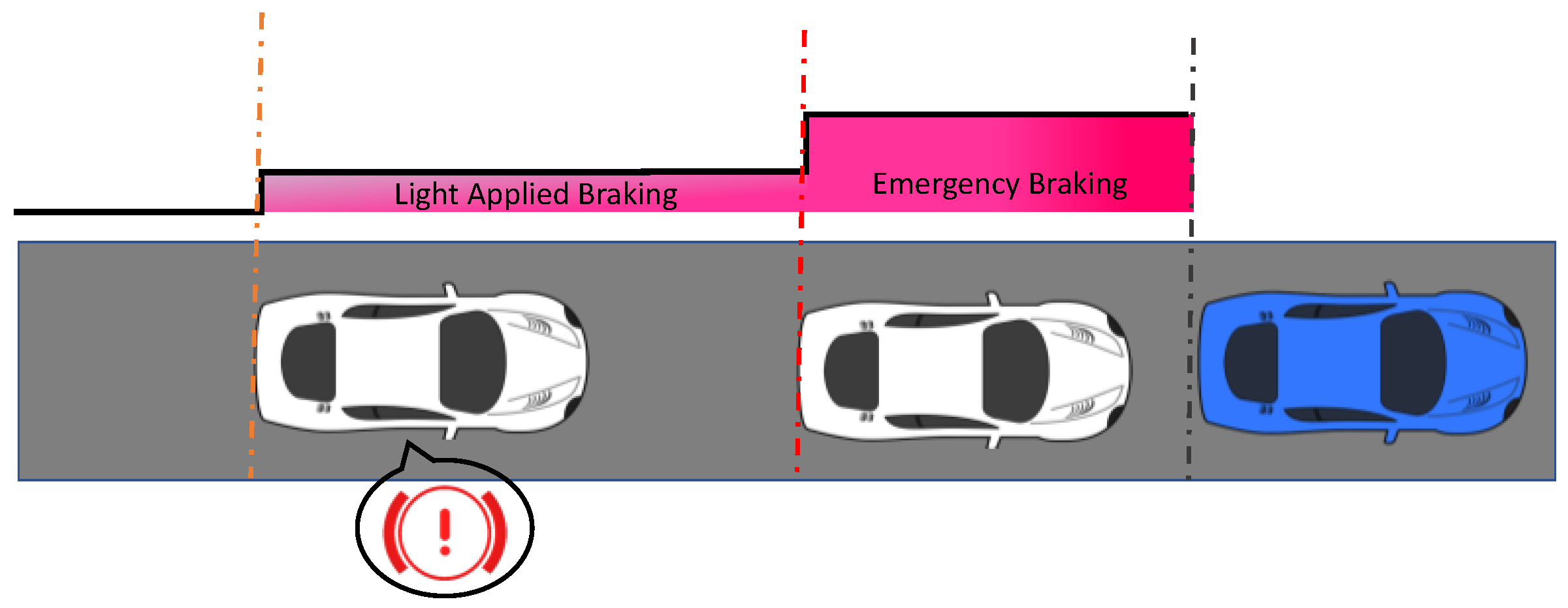
An advanced emergency braking system (EBS) with sensor fusion is proposed in this paper that can autonomously identify a probable forward collision and activate the vehicle forward collision warning (FCW) and braking system to brake the vehicle to avoid or mitigate a collision. If the system detects a risk of collision with vehicles or pedestrians at the front of the car, the driver will be notified by visual and aural alarms, and light, automatic brakes will be applied. This is to obtain the driver’s attention and get them to act quickly to prevent collisions. If the driver fails to decelerate and the likelihood of an accident increases, the system will automatically deploy emergency braking just before the crash. This will aid in avoiding or reducing the collision’s damage. If the driver applies the brakes, it can also enhance the braking force, but not enough to avoid a crash. Vehicles are detected by all AEBSs, and many of them can also identify pedestrians and bicycles. The nomenclature contains a list of abbreviations and symbols.

1.1. Emergency Braking System

AEBSs are among the best collision-avoidance systems you can have in your car, according to numerous studies from Europe and other nations. The Insurance Institute for Highway Safety and the Highway Loss Data Institute conducted one of the most recent studies in April 2019 and discovered a 50% decrease in front-to-rear collisions and a 56% reduction in front-to-rear road accidents with injuries for vehicles equipped with the forward warning and AEBS [4].

Modern technology commonly employs lidar, cameras, and radar to find obstacles in emergency braking situations systems. The faster the speed of the vehicle, the higher the chance that the AEBS will be able to stop it in time to avoid a collision. An essential part of automotive safety technology is an automated braking system [5]. It is an advanced technology that is intended to either prevent potential collisions or slow down a moving vehicle before hitting another pedestrian, or some other impediment or car. These systems use a combination of sensors, such as ultrasonic, video, infrared, or radar, to scan the area in front of the car for potential obstacles, and if any one of the obstacles is found, brake control is used to avoid a collision [6].

Although the technology for automated braking systems varies depending on the automaker, all technologies start with sensory input. The system that uses radar, lidar, or cameras, to check whether anything is in front of the car, varies from manufacturer to manufacturer. For instance, the system analyses the likelihood of a collision based on the traffic in front of the vehicle. If an object is found, the system keeps measuring the sensor data directly. The AEBS measures the distance between both the vehicle and the object moving in front of the vehicle and calculates their relative speeds. If the system concludes that the vehicle’s speed is greater than the speed of the identified item in front of the car, it can automatically apply the brakes to prevent a potential collision. An automated braking system can also communicate with a car’s GPS and use its database of traffic signs and other data to apply the brakes quickly if the driver does not [7].

The electronic control unit (ECU) on your car gives the AEBS access to additional data about it. The AEBS can evaluate whether the speed at which you are traveling has the potential to result in a collision by factoring in your vehicle’s speed and measuring the distance to the object detected in front of the vehicle. When an impending collision is identified, the AEBS will examine the braking systems. The AEBS will not step in if you have already applied the brakes and are slowing down sufficiently to avoid the crash. However, if you have not applied the brakes or have not done so with enough force because of the approaching obstacle or vehicle, the AEBS will take control and apply the brakes for you [8].

1.2. Sensor Fusion

The method to combine data from various cameras, lidars, and radars to create a single model or image of the area surrounding a vehicle is known as sensor fusion. As a result of balancing the strengths of the various sensor, the model that results is more precise. The data collected by sensor fusion can subsequently be used by vehicle systems to enable smarter actions [9].

Every sensor type or modality has advantages and disadvantages on its own. Even in adverse weather, radars are quite effective at calculating distance and speed, but they are unable to recognize the color of a stoplight or read street signs. Cameras are excellent at interpreting signs or categorizing objects such as humans, other vehicles, and bicycles. However, they are quickly dazzled (unresponsive) by debris, the snow, the light, the rain, or the night. Lidars are capable of precise object detection, but they lack the price and range of cameras or radars [10]. Some properties of vision, lidars, and radars are given below

Table 1. Main features of radar, lidar, and vision sensors.

Radar	Lidar	Vision
Long-range sensing	Precise 3D object detection	Object classification
Object movement	Range accuracy	Object angular position
All weather performance	Free space detection	Scene context

.

To create a more thorough and accurate environmental model, sensor fusion combines the data from all of these different types of sensors, or a highly variable collection of sensor modalities. By using a technique called internal and exterior sensor fusion, it may also correlate with the information obtained from the environment [11]. The information from numerous sensors of the same sort, such as radars, might also be combined by a vehicle via sensor fusion. Trying to take advantage of slightly overlapping areas of view enhances the experience. More than one sensor will pick up things simultaneously when more than one radar scans the area around a vehicle [12].

The detection likelihood and reliability of things nearby the vehicle can be increased by fusing or overlapping the detections from those various sensors when interpreted by global 360° perception software, which also produces a more accurate and trustworthy picture of the environment. The most fundamental distinction between centralized and decentralized sensor fusion is made by the data being used, the raw sensor data, the features extracted from the sensor data, and the judgments made by utilizing the extracted features and other information. Depending on how it is used, sensor fusion may have the following advantages:

• Improved data dependability
• Improved data quality
• Estimate the unmeasured states
• Expanded coverage

Radar or vision-based systems are frequently employed in previously built systems, and the implementation of an AEBS can be conducted in MATLAB and Simulink. The suggested technique uses sensor data fusion from radars, vision, and lidars. The fundamental form used to track automobiles, people, or any obstacle in good or bad weather is the sensors model, which is based on the acquisition of MATLAB and Simulink. Three advanced sensor-based sensor fusion techniques are proposed, which are included by the MATLAB model in the emergency braking procedure. In contrast to earlier linear systems, our advanced system also features a non-linear super twisting speed controller which also supports EBS.

This paper aims to demonstrate stable AEBS operation to avoid or minimize forward collisions and prevent accidents while any vehicle is identified. In Section 2, the existing AEBS and fusion methods that have been applied in this field are discussed. The research and methodology are covered in Section 3, a simulation is discussed in Section 4, Section 5 consists of Results and Discussions, and Section 6 and Section 7 consist of a comparison with the existing research and the conclusion, respectively.

2. Literature Review

The article [13] presents a recognition model for the front wheel of the car which is dependent upon the backpropagation (BP) neural network and hidden Markov model. In this proposed system, the inputs included are the brake pedal, accelerator pedal, and vehicle speed data, which are used to examine the driver’s intention. An AEB model for the following vehicle is suggested that may dynamically adjust the critical braking distance under varied driving circumstances to avoid rear-end collisions, according to the recognized driver’s intention provided through the Internet of Vehicles. In [14], based on model predictive control (MPC) theory, a variable time headway autonomous emergency braking (AEB) control method is suggested. This kind of interference is addressed by the variable time headway-based safety distance model. The AEB controller is designed with collision avoidance, driver characteristics, and ride comfort variables in mind. The variables used to build the state equation are the separation between the two vehicles, their relative velocities, and the ego vehicle’s velocities and accelerations.

The authors in [15] describe the new moving object identification and tracking system, which builds on and improves the previous system developed for the DARPA Urban Challenge in 2007. The author updated the previous motion and observation models to include active sensors and vision sensors. The vision module in the new system recognizes bikers, pedestrians, and cars and generates a vision target for them. This visual recognition information is used by the proposed system to improve the tracking prediction, data association, and motion categorization of the previous system.

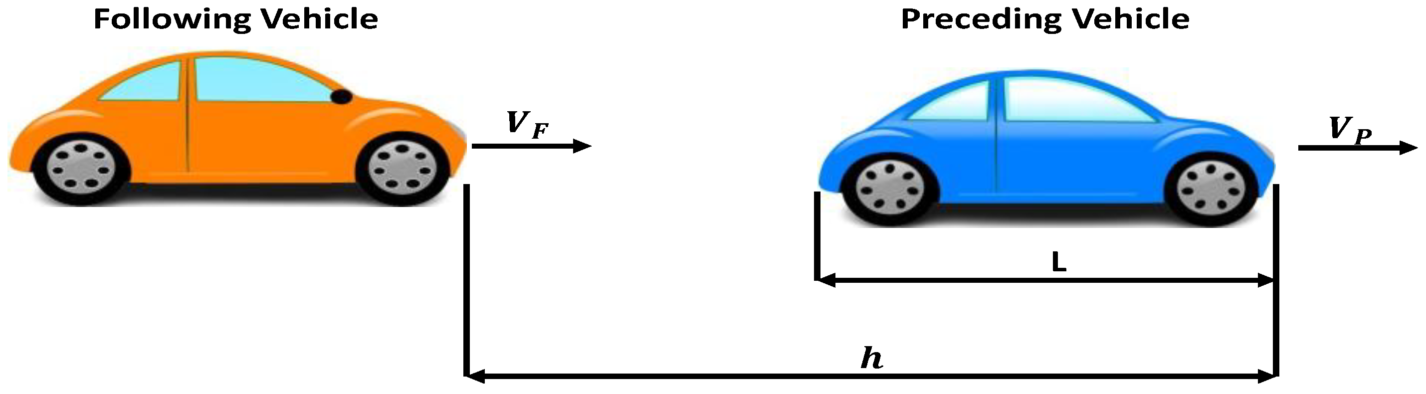
The purpose of [16] was to investigate the design and operation of an AEBS using the many fundamentals of mechanical and electronic engineering, commonly referred to as Mechatronics. An ultrasonic sensor combined with a stereo camera identifies an impediment in front of the car and provides information about the relative distances between the object and the vehicles in this system. The ECU will then determine whether or not an accident is likely to occur, and the brake will be deployed autonomously as a result of this approach. Time-to-collision (TTC) is one of the most extensively used time-based approaches presented in [17], and it was designed to evaluate the time it will take for an accident occurs between a previous and accompanying vehicle. In Figure 2, a summary of the TTC algorithm is presented.

The TTC was used to calculate the remaining time for two vehicles to collide [18]. The following is how the TTC algorithm is calculated.

$$\mathrm{TTC}=\frac{\mathrm{h}-\mathrm{L}}{{\mathrm{V}}_{\mathrm{P}}-{\mathrm{V}}_{\mathrm{F}}}$$

(1)

In Equation (1), h stands for the distance between the preceding and following vehicles, VF and VP stand for the speed of the following and preceding vehicles, and L stands for the length of the preceding vehicle.

To address the shortcomings of the previous method, the researchers proposed new stopping distance-based algorithms (SDAs) [19]. Calculating a safe stopping distance is one of the most effective ways to keep an eye on the possibility of a rear-end accident. SDA-based techniques for assessing rear-end collision risk are based on the assumption that in a car-following position, the leading car’s friction coefficient must be higher than the pursuing cars. An overview of the SDA is shown below in Figure 3 [20].

When stopping at a given speed, longer reaction times increase the thinking distance; however, collisions can occur in this algorithm with shorter reaction times and faster decision times [21]. Based on non-parametric techniques, many scholars have sought to construct collision-warning solutions. Artificial Neural Network (ANN)-based technology is one of the most important new technologies in the rear-end collision warning system (CWS). The advantage of the ANN-based approach is that it can deal with solving complex unobservable problems. Initially offered in [22] was a vehicle control strategy for multi-directional collision avoidance.

Numerous researchers have tried to develop collision-warning systems based on non-parametric methods because the prior parametric deterministic approaches have the drawback that they do not represent the influence of PRT. ANN-based technology is one of the most important new technologies on the back-end CWS. The advantage of using an ANN-based approach is that it can deal with handling complex unobservable problems. Initially suggested in [23] was a vehicle control strategy for multi-directional collision avoidance. The multi-layer perceptron neural network and fuzzy logic algorithms, respectively, were used in this study. More recently, a method to integrate fuzzy logic and neural networks was meant to create an algorithm that operates a car on the highway based on highly accurate GPS data [24].

The authors in [25] developed an algorithm for making decisions for AEB pedestrians using radar and camera sensors for the data fusion technique. The EuroNCAP protocol’s potential collision avoidance scenarios were examined and a reliable pedestrian tracking method was suggested. By creating the system activation zone with the relative speed and potential distance needed to stop pedestrians, as well as by utilizing a brake model to anticipate the collision avoidance time, the performance of the AEB system was improved. In [26], a MATLAB-created AEBS module, based on two radar sensors, was suggested. The proposed AEBS depends on a short-range and long-range radar, the time between the detection of the obstacle in front of the autonomous vehicle, and the speed of the autonomous vehicle.

In [27], an autonomous vehicle collision avoidance and pedestrian detection system was proposed based on stereo vision. It monitors the area using two cameras that are placed at a set distance apart. When a pedestrian is detected, the system estimates the stopping distance, and the suggested controller algorithm will initiate braking if the calculated distance is less than the safe driving distance. Using an infrared camera that can detect heat and lidar sensors in RC cars for obstacle detection, ref. [28] proposed a new obstacle recognition method for accurately identifying front cars and pedestrians and reducing the danger of vehicle collisions in bad weather. By using RC cars as testbeds for autonomous vehicles, the author showed that the suggested technique is feasible by integrating lidars and a thermal infrared camera on vehicles.

In [29], a new method to determine the distance (Hurdle Detection) was proposed for a secure environment within a moving vehicle. Eight ultrasonic sensors are employed in this system to detect various object types. The car and sensor are allowed to function normally up to the sensor detecting a potential risk by putting into practice a potential increase in the safety system in the vehicle. The literature review suggests that the existing system employed one or two (mostly radar and vision) types of sensors for data fusion with various EBS controller algorithms. Existing obstacle identification fusion technologies have resulted in major accidents because they cannot effectively identify vehicles or pedestrians at night and in bad weather. False positives of any sensor are also drawbacks of the previously existing AEB systems that may cause disruptions or accidents.

In this paper, our contribution is to introduce a dependable multi-sensor fusion architecture and a reliable decision-making algorithm for the AEB controller to perform autonomous emergency braking and protect pedestrians. The proposed multi-sensor fusion architecture has three different types of sensors: radar, lidar, and vision sensors. The TTC and stopping time calculation approaches are used to implement the AEB controller and FCW algorithm. A non-linear speed controller is included in place of existing linear controllers in addition to supporting AEB. Additionally, a suitable collision decision and prediction algorithm is created and carefully investigated for the EuroNCAP AEB pedestrian situations. This system also managed the trade-off between AEB performance and false positives by setting the threshold for AEB activation and cautiously preventing false positives to achieve an accurate performance of the system.

3. Research Methodology

An advanced active safety system to protect vehicles from collisions is the AEBS. It is made to assist drivers in preventing or lessening crashes with other drivers on the road. The Simulink model of MATLAB was used to implement the AEBS. The implementation of an EBS can be performed in MATLAB and Simulink and the radar and vision-based systems were widely used in the previously implemented system, but the proposed system uses lidar, radar, and vision with sensor fusion. The sensors model based on the acquisition of MATLAB and Simulink was used as a basic form to track vehicles, pedestrians, or any hurdle in both good and bad weather. In the case of the emergency braking process, three advanced sensors based on the sensor fusion method were projected and incorporated by the model provided by MATLAB [30,31].

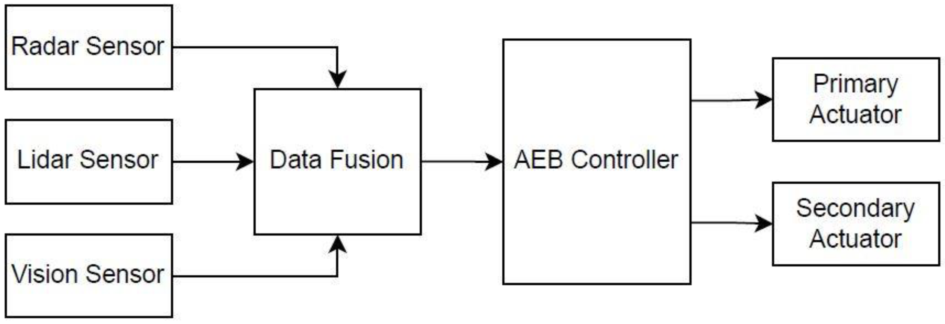
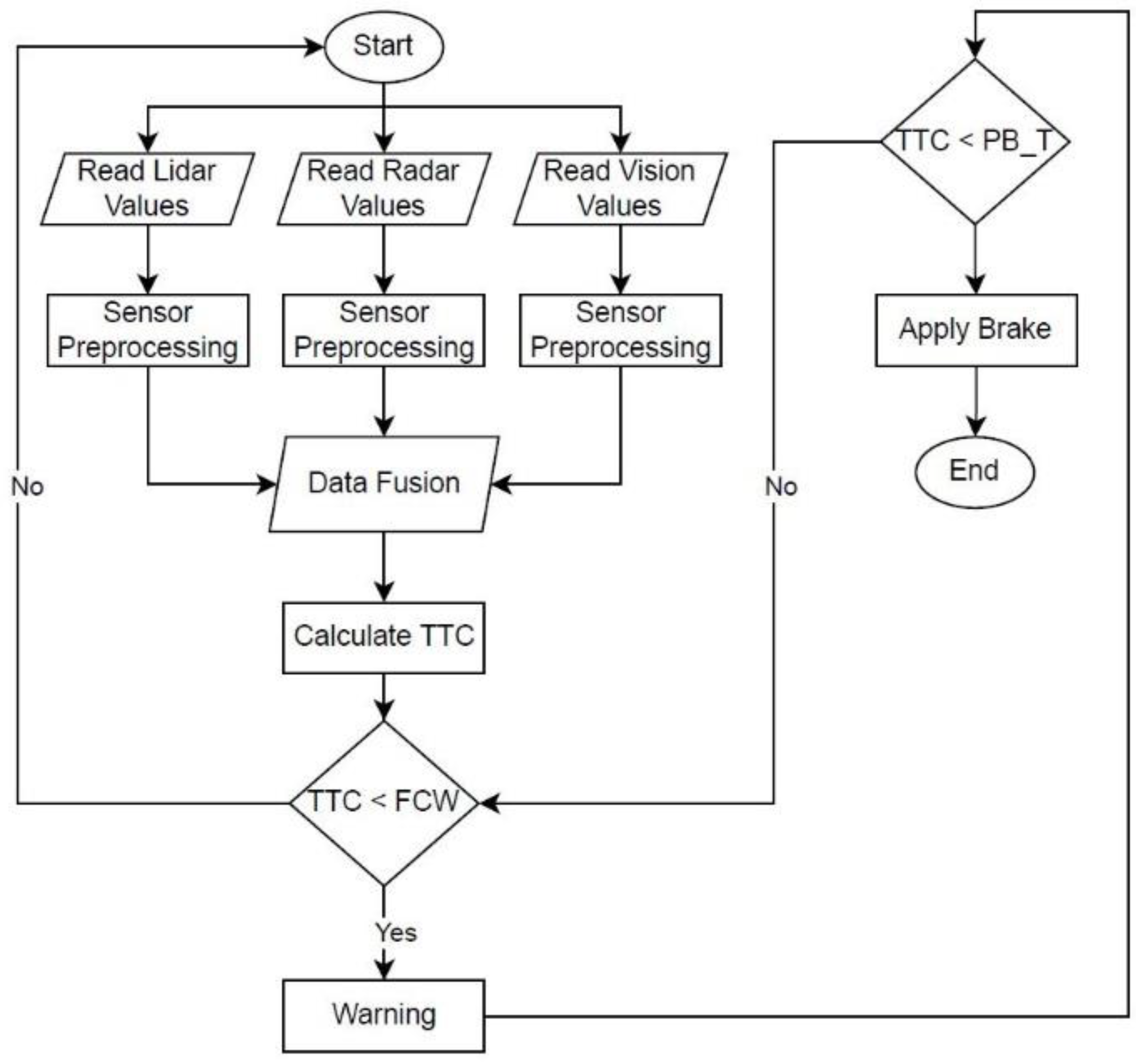
At the start, three sensors radar, vision, and lidars detect and track objects near the ego vehicle. When an ego vehicle approaches a leading vehicle, the sensor measures the ego vehicle’s distance from the leading vehicle, calculates the speeds of both vehicles, calculates the time to collision, activates the forward collision alert, and then calculates the stopping distance. When the lead vehicle’s TTC is less than the TFCW, the FCW alert is activated. Due to distractions, the driver may fail to engage the brakes; in this situation, the AEBS operates autonomously to avoid or lessen the impact. All the processes are shown below in the flow chart and block diagram in Figure 4 and Figure 5.

Our proposed system is divided into two parts: sensor fusion and AEB control. First, the AEB algorithm’s control system is divided into two primary subsystems, the AEB control subsystem, and the speed control subsystem, both of which are illustrated in this section. The AEB control subsystem is responsible for conducting vehicle braking, while the speed control subsystem is in charge of accelerating the vehicle. This study only examines the scenario in which the leading and ego cars both move in the same lane.

3.1. AEB Controller

The AEB controller subsystem uses a stopping time calculation method to implement the AEBS controller and FCW algorithm. The stopping time can be described as follows:

$$T_{stop}=v_{ego}/a_{brake}$$

(2)

where the $T_{stop}$ stopping time is the period from the ego vehicle’s first deceleration to when it comes to a complete stop. Additionally, $a_{brake}$ is the ego vehicle’s deceleration at this point in the deceleration cycle.

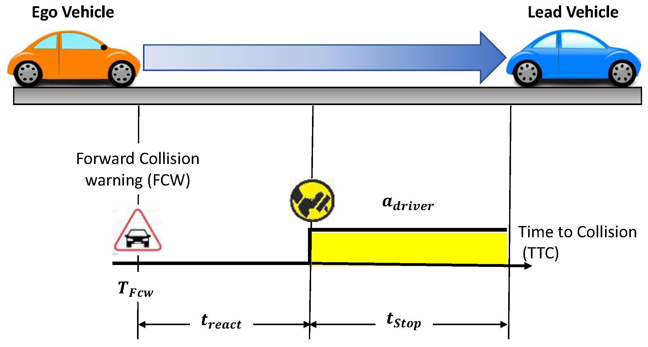
As seen in Figure 6, drivers are warned by the FCW system that a collision with the lead vehicle is impending and that they should apply the brakes with a delay in the time indicated $T_{react}$. The following equation can be used to determine how far the ego vehicle will go before colliding with the lead car:

$$T_{FCW}=T_{react}+T_{stop}=T_{react}+v_{ego}/a_{driver}$$

(3)

where $a_{driver}$ is the ego vehicle’s deceleration and is the ego vehicle’s velocity.

The AEB controller subsystem consists of three functions: AEB Logic, $\mathit{StoppingTimeCalculation}$, and TTCCalculation. The FCW can be engaged when the FCW is greater than the TTC of the ego vehicle, as represented in Equation (4). The AEBS takes over the operation of the car instead of the driver if the driver does not react to the alert on time.

$$T_{ttc}=x_{relative}/v_{relative}$$

(4)

Here, the lead car’s velocity toward the ego vehicle is the $v_{relative}$, and the $x_{relative}$ is the distance between the two vehicles.

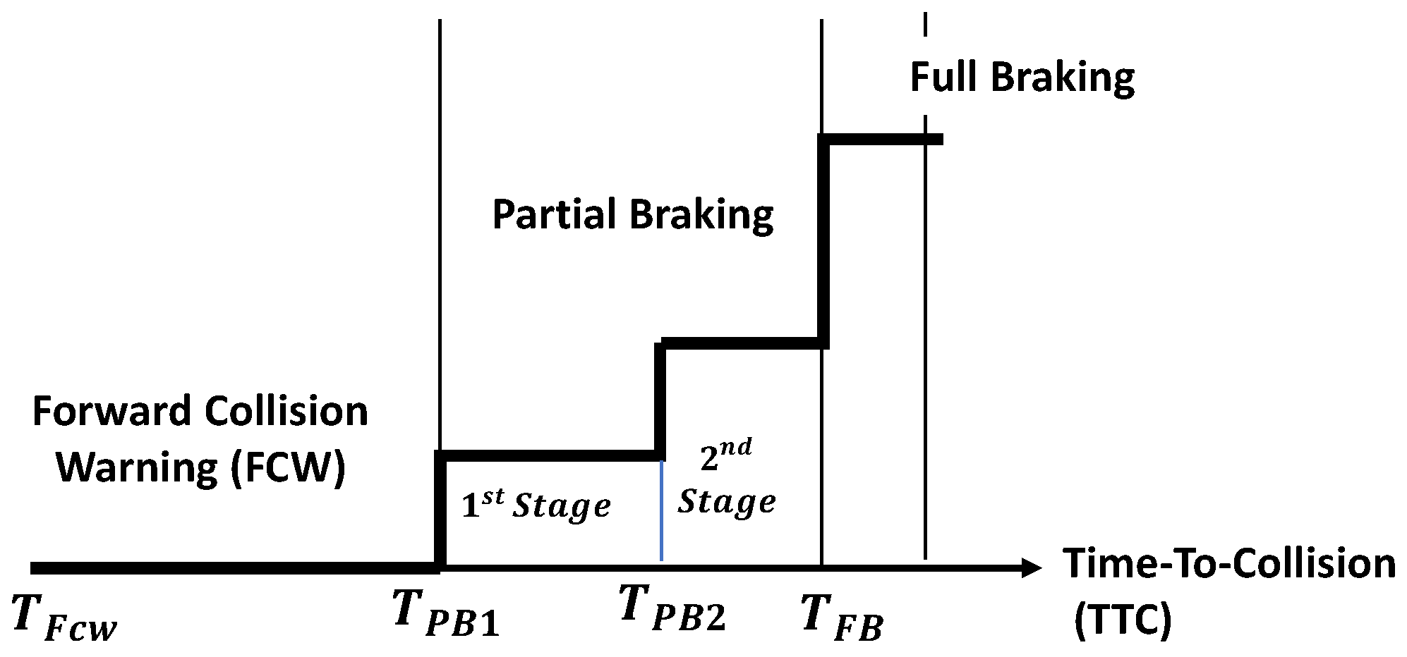
The cascaded braking method used by the AEBS is depicted in Figure 7. The two stages of partial braking (PB) and full braking (FB) make up the cascaded braking.

Equation (3) in $StoppingTimeCalculation$ is used to determine the stopping period for the FCW, and both the initial and second phases of PB and FB are calculated in the manner described below:

$$T_{PB1}=v_{ego}/a_{PB1}$$

(5)

$$T_{PB2}=v_{ego}/a_{PB2}$$

(6)

$$T_{FB}=v_{ego}/a_{FB}$$

(7)

where $a_{\mathit{PB}1}$, $a_{PB2}$, and $a_{\mathit{FB}}$ represent, respectively, the deceleration of both the first and second stages of PB and FB. An AEBS is a function that compares the stopping time calculated by $StoppingTimeCalculation$ to the TTC to decide if the FCW or which stages of the brakes can always be engaged.

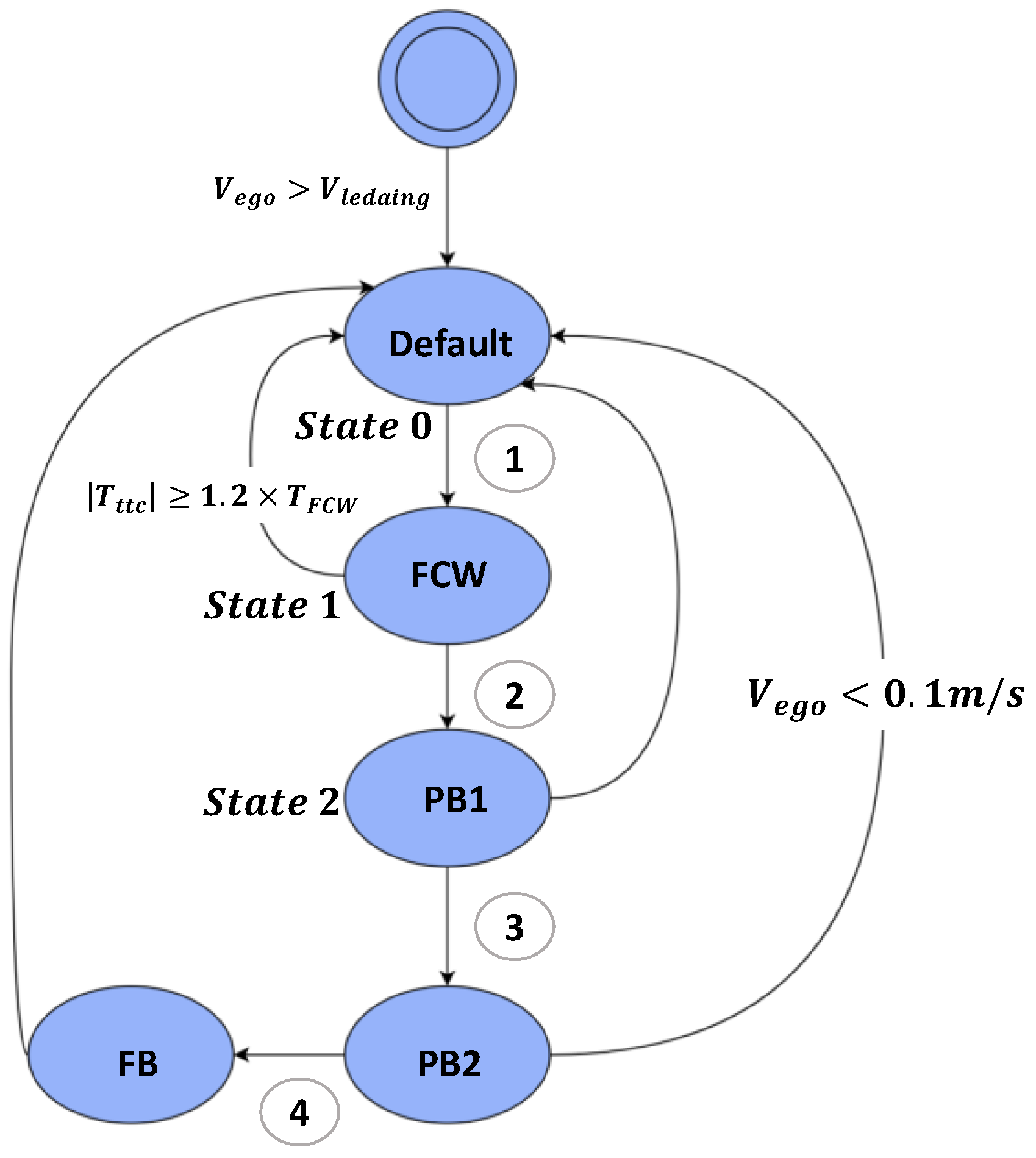
The state chart AEBS is shown in Figure 8. State 0 through State 4 in this diagram, respectively, refer to the following states [13]:

State 0:

The default state, in which the ego vehicle maintains its pre-determined speed (when the preceding condition is State 4, set the preset velocity to 0).

State 1:

The FCW is enabled and alerts the driver to apply the brake.

State 2:

The activation state of PB1. At this point, the ego vehicle begins to slow down and the deceleration is 3.8 m/s².

State 3:

The activation state of PB2. At this point, the ego vehicle begins to slow down and the deceleration is 5.8 m/s².

State 4:

The activation state of FB. At this point, the ego vehicle begins to slow down and the deceleration is 9.8 m/s².

The following circumstances, which are indicated in Figure 8 givens in Equations (8)–(11), cause the ego vehicle’s state to change:

$$0>T_{ttc} and T_{FCW}>\left|T_{ttc}\right|$$

(8)

$$0>T_{ttc} and T_{PB1}>\left|T_{ttc}\right|$$

(9)

$$0>T_{ttc} and T_{PB2}>\left|T_{ttc}\right|$$

(10)

$$0>T_{ttc} and T_{PB3}>\left|T_{ttc}\right|$$

(11)

The ego vehicle accelerates to attain the defined velocity after the driving scenario has been started, and if the defined velocity is reached, it maintains the velocity. The car in front of the ego vehicle is detected by the radar, lidar, and vision sensors, which extract data. As soon as requirement 1A is satisfied, the FCW is turned on. Until condition 2A is satisfied, the ego vehicle remains in State 1 in motion. Starting at this point, the ego vehicle applies cascaded brakes. Similar to this, the ego car is in Stage 3 or 4 when condition 3A or 4A has been satisfied.

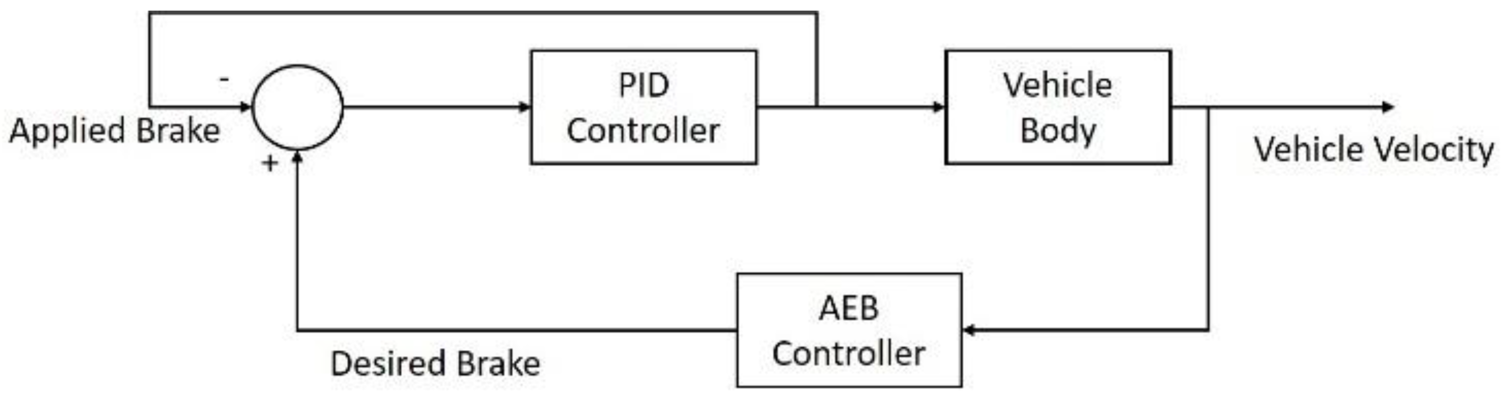
The ego vehicle begins to decelerate as soon as it enters the braking stage and continues to do so until its speed is less than 0.1 m/s. There are two PID controllers in this research, as indicated below. During the acceleration phase, one is in charge of regulating the ego vehicle’s speed (State 0). The other is used as leverage to manage the ego vehicle’s braking stage deceleration (State 2–4). The second PID controller is the part of the AEB controller which controls the different stages of braking, as shown in below Figure 9. The implementation of this controller was conducted in a simulation using a signal flow graph where the controller decides on which declaration rate to apply for the desired velocity and braking condition.

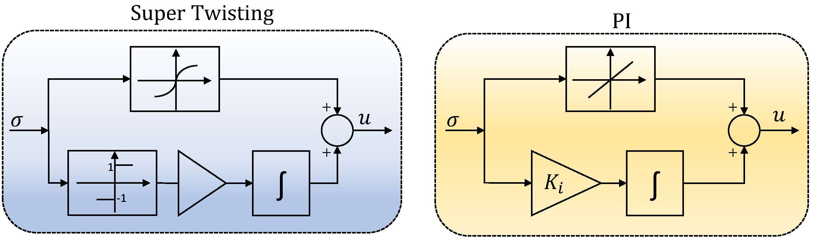
3.2. Speed Controller Subsystem

Scholars from all around the globe have worked hard to find solutions to the issues raised by conventional proportional-integral (PI) control, and some recent advances in control theory, active disturbance rejection control, neural networks, and fuzzy control, including adaptive control and the SMC, have been successfully applied to the speed control system of the super twisting sliding mode controller (ST-SMC). Because of its dependability, quick dynamic reaction, and ease of implementation, the SMC is one of those that are frequently employed. Although the traditional sliding mode control increases the system’s robustness, it is simple to cause the system chattering phenomenon and lower the dynamic quality of the system when it is applied to the actual system because of the switch’s time delay and spatial lag, state detection error, and other factors.

Super Twisting Sliding Mode Controller

The conflict between system chattering and attaining speed is resolved by the high-order sliding mode method. The super twisting algorithm, in contrast to other high-order sliding mode algorithms, does not require the sliding mode surface and its derivative to settle to zero instantaneously, preventing the need for complicated noise management law construction.

The ST-SMC, created specifically for systems with a relative degree of one, is a workable substitute for the traditional first-order SMC without compromising tracking performance or chattering. This method describes a direction that resembles one of its twisting algorithms and converges in a finite amount of time with the appropriate parameter choices.

The standard PI controller shown in Figure 10 is a non-linear variant of the ST method. The ST-SMC is more robust to the output amount of noise and potential estimate errors, making it particularly well suited for practical application. Two terms make up the ST-SMC control law u(t). The second term is the sliding variable continuous function that is available and is only present during the reaching phase, whereas the first component is described by the discontinuity of the derivative concerning time. The control algorithm is defined by the following control law [32].

$$u\left(t\right)=\dot{U_1\left(t\right)+U_2\left(t\right)}$$

(12)

$${\dot{u}}_1\left(t\right)=\{\begin{array}{c}-u\\ -Wsign\left(\sigma \right)\end{array} \begin{array}{c}if \left|u\right|>1\\ if \left|u\right|\le 1\end{array}$$

(13)

$$u_2\left(t\right)=\{\begin{array}{c}-\lambda \left|{\sigma }_0\right|\rho sign\left(\sigma \right) \\ -\lambda \left|{\sigma }_0\right|\rho sign\left(\sigma \right)\end{array}\begin{array}{c}if \left|\sigma \right|>{\sigma }_0\\ if \left|\sigma \right|\le {\sigma }_0\end{array}$$

(14)

where u is the boundary control value, ${\sigma }_0$ is the boundary layer surrounding the sliding surface σ, and W, λ, and ρ are control gains. In our controller, u is the output that controls the acceleration, and the inputs of the controller are σ and the error or distance between the sliding surface and our current value. The proposed speed controller in the system based on the ST-SMC accelerates the vehicle in normal conditions to its desired velocity and when braking is applied. Under this condition, the speed controller decelerates the vehicle using a throttle to support the EBS.

3.3. Sensor Fusion

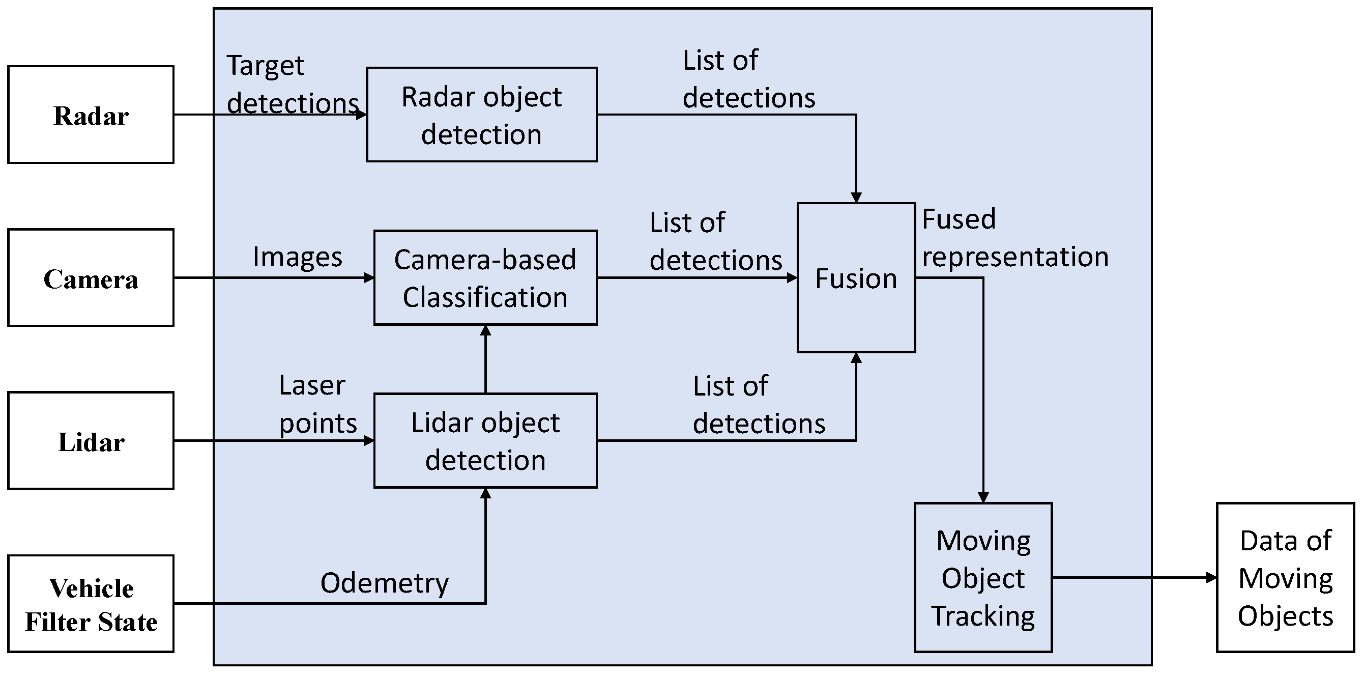
One of the most difficult parts of the area of autonomous vehicles is the identification and tracking of moving objects. The performance and ratability of the solutions are vital since tackling this challenge is essential for autonomous driving. As a result, it is usual for the car to use all of its installed sensors. The most well-liked method uses data from lidars, radars, and cameras to create sensor fusion. Early methods for the detection and tracking of moving objects concentrated on combining sensor data after tracking with additional data from a simultaneous localization and a mapping module. For a more comprehensive understanding of the processes, additional fusion was performed at the track level.

An innovative method in this research area combines detection from the lidar and radar levels with the camera-based classifier after feeding regions of interest from the lidar point clouds into it. The tracking module receives its data from the fusion module, which is used to create a list of moving objects. The perceived model of the world is enhanced by including the object classification from various sensor detectors. Figure 11 displays a block diagram of the various sensors perception system.

Instead of processing the data through a system to obtain object information or to extract features, restricted fusion is often used to pre-process lidar and radar data in a sensor fusion, combining camera, lidar, and radar sensors data. The combined data are then added to high levels of blocks of fusion that incorporate camera input. In this situation, high-level fusion produces the detection and classification while low-level fusion addresses the mapping and localization method. To make a high-level fusion by combining the low-level fusion as inputs may be one perceived trend in an autonomous vehicle.

The movement classification and effectiveness of the data association can be enhanced by using visual shapes and information about the object class when choosing an object detection method. A tracking system can alternate between the 3D box and point representations depending on how far the object is from the vehicle. This means that camera data are essential for localization and tracking activities as well. In the future, tracking systems will be able to track more accurately thanks to the exploration of contextual data about urban traffic surroundings.

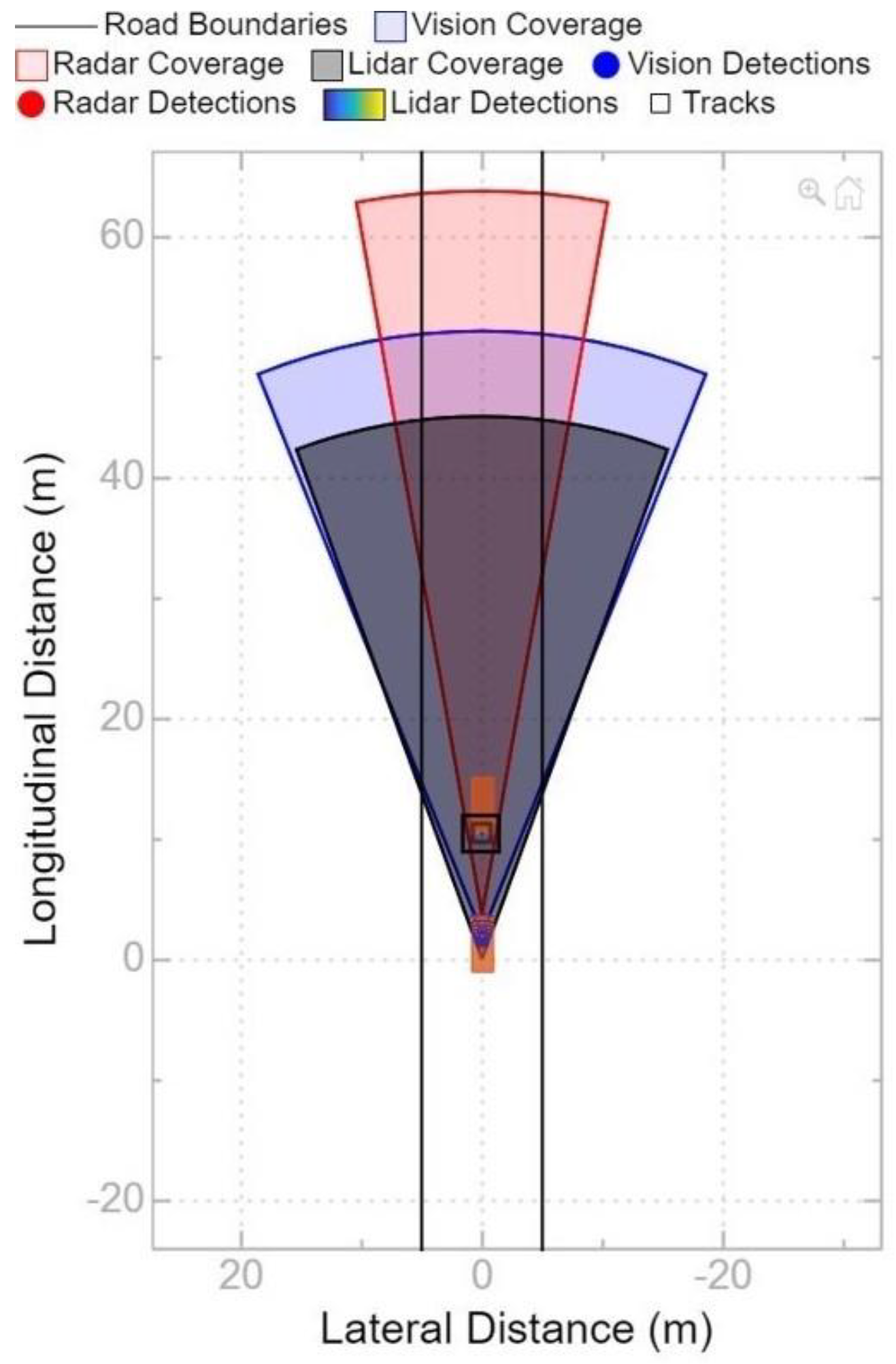
A camera can also provide information about its width and height, estimated speed, and relative position. The test vehicle’s relative velocity to an object moving forward can be determined using radar. The ability of a radar sensor to detect a car is good, but it does not do well when a pedestrian is present. The precise relative distance, estimated velocity, object class, and breadth and height can all be determined with the lidar. The test vehicle with the three different sensors and leading vehicle detected is shown in the below-given Figure 12.

The relative distance and relative velocity of the item are the details needed in this study for data fusion. Equations (15)–(18) explain the measured data z(k) at time step k.

$$z\left(k\right)=\left\{z^v\left(k\right),z^R\left(k\right),z^L\left(k\right),\right\}$$

(15)

$$z^v\left(k\right)=\left\{v_1,v_2,\dots ,v_p\right\} v_i={\left[x y \dot{x}\right]}^T i=1,\dots ,p$$

(16)

$$z^R\left(k\right)=\left\{r_1,r_2,\dots ,r_q\right\} r_i={\left[x y \dot{x}\right]}^T i=1,\dots ,q$$

(17)

$$z^L\left(k\right)=\left\{l_1,l_2,\dots ,l_r\right\} l_i={\left[x y \dot{x}\right]}^T i=1,\dots ,r$$

(18)

Here, $z^v\left(k\right)$, $z^R\left(k\right)$, and $z^L\left(k\right)$ denote the measured value of the vision, radar, and lidar at time step k, respectively. The distances of each sensor are denoted by y, x shows the longitudinal distance, $\dot{x}$ is the relative velocity, and p, q, and r are the total number of objects that the sensors have identified. Every time a measurement is updated, a multi-rate Kalman filter (KF) is employed to account for the timing variances of each of the sensors. The measurement is updated by one sensor at its own update time, and the remaining sensors’ measurements are then estimated using the KF until the subsequent measurements. The sensor fusion’s update rate is time synchronized with the control loop.

Using three different types of sensors, the vehicle can track obstacles through multi-sensor data fusion. Effective track-to-track data fusion is implemented through decentralized data fusion. Each sensor’s ability to identify objects is tracked using a fusion algorithm.

$${\widehat{x}}_k={\left[x y \dot{x} \dot{y}\right]}^T$$

(19)

where y and x are the lateral and longitudinal relative distances, respectively, and $\dot{x}$ and $\dot{y}$ are the leading vehicle’s relative velocity.

There is a validated track-to-track management for each tracker. By fusing the data, the precision of the integrated state value can be increased. The lateral velocity ${\dot{y}}_k^V$ and azimuth angle $({\theta }_K^V)$ of the vision sensor, along with the longitudinal velocity $({\dot{x}}_k^{LR})$ and distance ($x_k^{LR}$) of the radar and lidar, are thought to be the most important variables. Equation (20) can be used to explain the fusion track (${\widehat{x}}_k^{VLR}$) of the radar (R), lidar (L), and vision (v).

$${\widehat{x}}_k^{VLR}=\left[\begin{array}{c}{x}_k\\ \begin{array}{c}{y}_k\\ {\dot{x}}_k\\ {\dot{y}}_k\end{array}\end{array}\right]=\left[\begin{array}{c}{x}_k^{LR}\\ \begin{array}{c}{x}_k^{LR}\times \tan {\theta }_k^V\\ {\dot{x}}_k^{LR}\\ {\dot{y}}_k^V\end{array}\end{array}\right]$$

(20)

4. Simulation

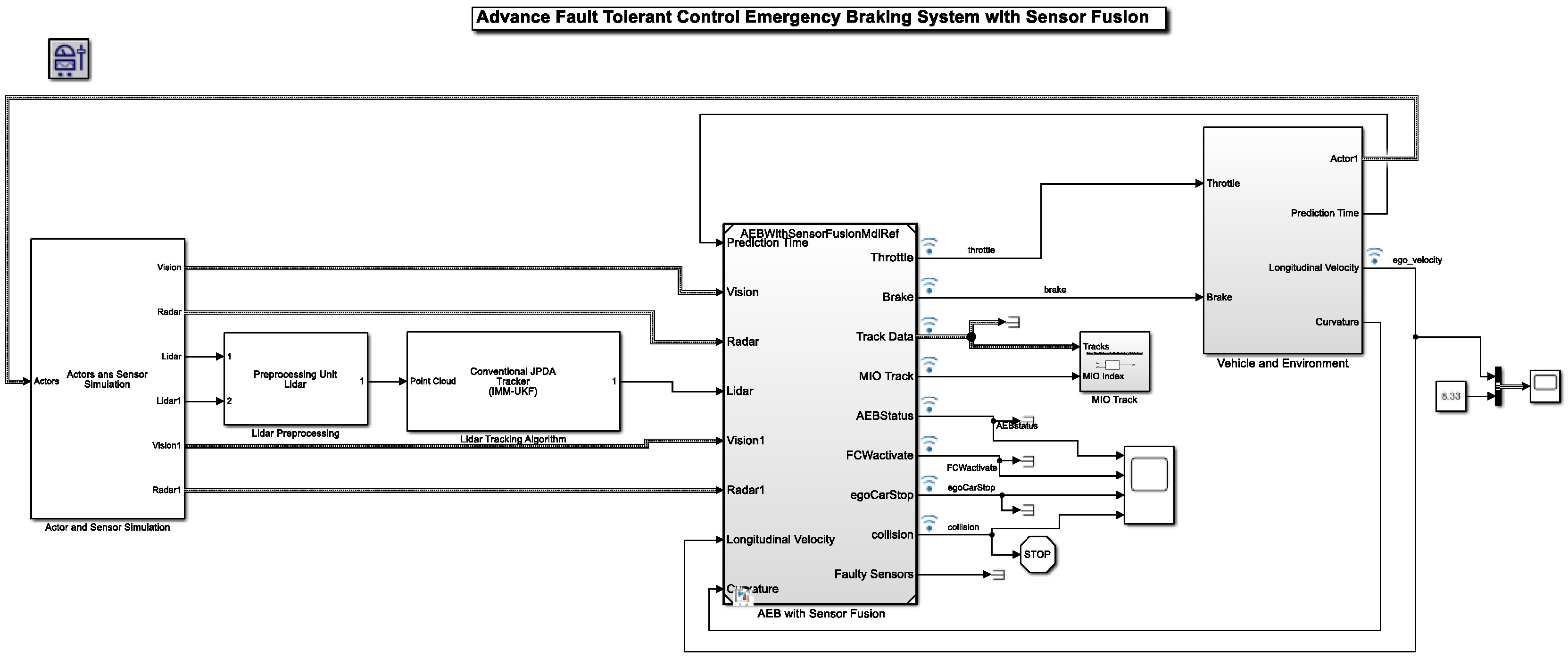
The Simulink diagram of the suggested model is shown in Figure 13. The sensors and actuators, roads, lidars, cameras, and radar sensors utilized in the simulation were all specified by this subsystem. The raw data were pre-processed to extract items in the lidar tracking algorithm subsystem model. The AEBS with a sensor fusion block had a computation system that included vehicle detection systems from the camera, radar, and lidar sensors, and it specified the longitudinal and lateral evaluation logic that gave the control system acceleration controls, information about the ego vehicle reference path, information about the most important object, and the steering angle. The ego vehicle was modeled by the vehicle dynamics subsystem using a bicycle simulator, and its status was maintained using instructions from the AEBS controllers model.

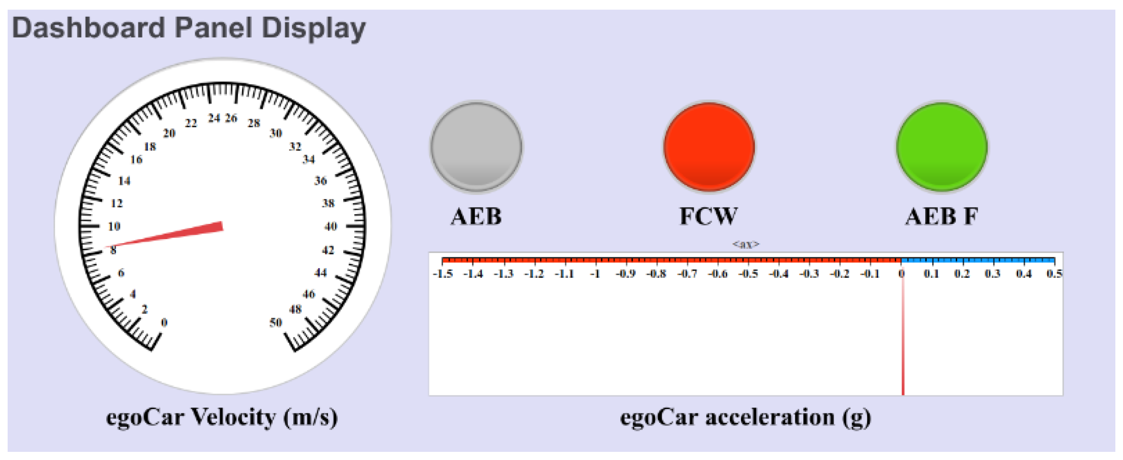
A scenario was created and it included one leading vehicle and an ego vehicle. A straight road was implemented with a standard width, a custom figure window to plot the scenario, and the stop time for the scenario was set to the required seconds. The cars were set up in a driving scenario, the all-set driving scenario object was imported into the Driving Scenario Designer App, and the results were exported. In the proposed system, a dashboard display in the vehicle similar to that in Figure 14 was present. The purpose of the dashboard is to warn drivers when the FCW state activates and to inform them about the braking status of the vehicle during first, second, and fully braking.

5. Results and Discussion

In the proposed system, radar, lidar, and vision sensors are used with various angular views for the simulation utilizing the AEBTestBench module so that the simulation’s field of coverage will be greater. The model consists of two primary subsystems. The first is the research part, which includes the AEB with a sensor fusion and AEB controller. The second part of the system is Environment and Vehicle, which mimics the dynamics of the ego vehicle and the surrounding environment. Driving scenario readers, lidar point cloud producers, and radar detection generators all give synthetic sensor data for the objects. The AEB controller is used to compute the stopping time and implements the AEB control algorithm and the FCW in accordance. This model is intended to run for 6 s in order to check each result. The reaction time of the system is 0.1 s. For instance, in a simulation, if a vehicle is spotted by sensors and the conditions (0 > T_ttc and T_FCW > |T_ttc |) hold, the system will generate an alarm or warning within 0.1 s.

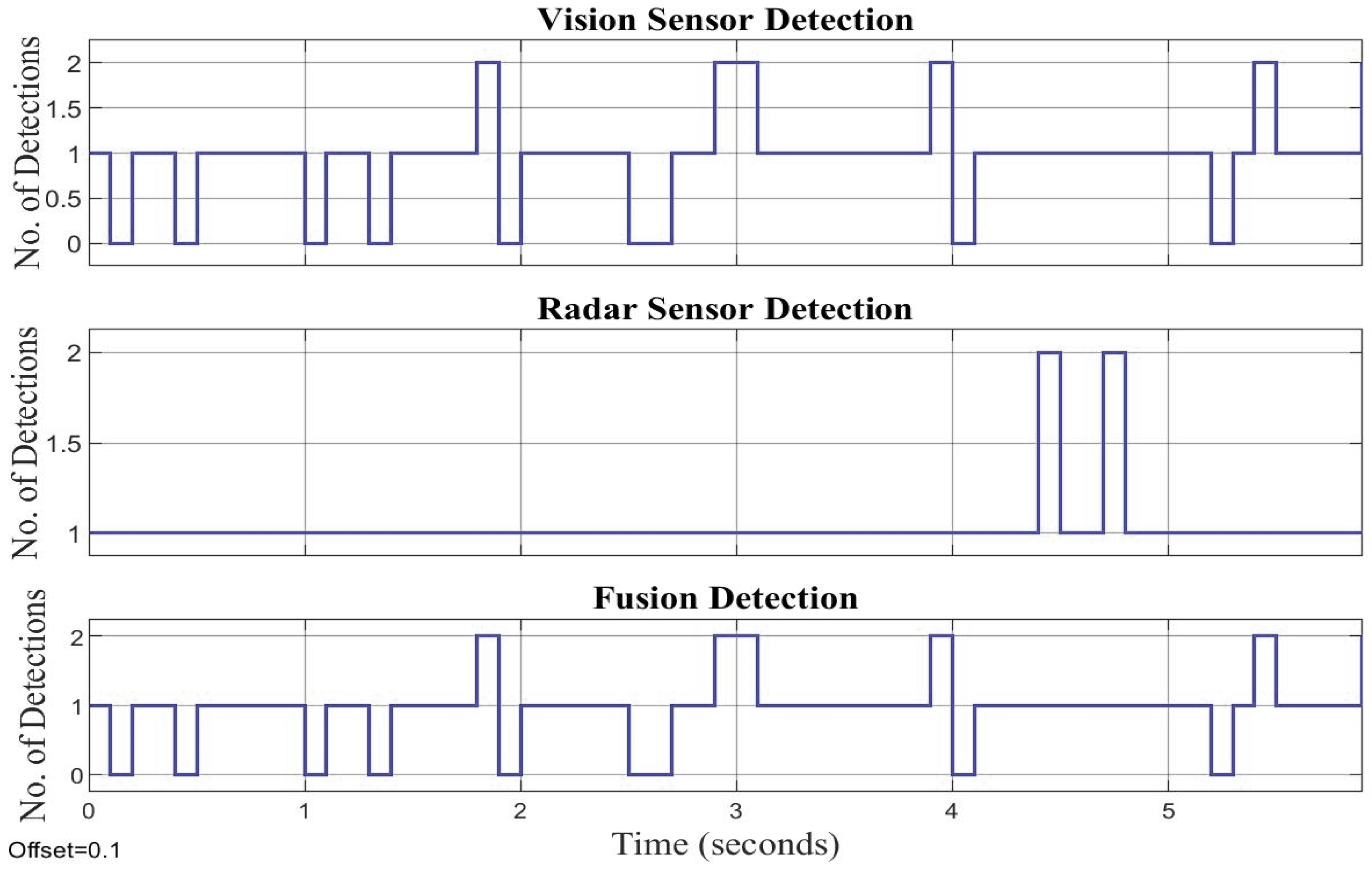
Figure 15 shows the observed number of lidar, vision, and radar sensor detections in addition to the computed sensor fusion result detections. The number of detections represents the quantity of the leading vehicle tracks that the sensors have detected. The track-to-track fuser block and data concatenation are used to implement the fusion method. The block receives data from the cuboid lidar, rectangular lidar, rectangular radar, and rectangular vision detection and outputs fused tracks. The data concatenation block creates a single-track bus by combining the number of detections from all the sources. Using the Source-Config variable through the Pre-Load-Function callback, the fuser source configuration for the radar, lidar, and vision is set. Track fusion is represented in this graph at a single time step. The fact that the fused tracks are more accurate and precise than the individual sensor detections shows that the fusing of the detection estimates from all three sensors improves track accuracy. Fusion detection is utilized for additional computations. In this scenario, all the sensors are healthy; no error is found in any sensor. The stopping time is the period from when an ego vehicle first decelerates by using its brakes until it comes to a complete stop. The stopping time is calculated mathematically using Equation (2). When the FCW system alerts a driver that a collision with the lead vehicle is imminent, they are required to react to the alarm and to apply the brake during the delay period. Equation (3) gives the total distance that the ego vehicle must travel before colliding with the lead vehicle.

The TTC of the leading vehicle must be smaller than the TFCW for the FCW alert to be activated. The AEBS reacts automatically to prevent or decrease the impact of the collision when a driver fails to apply the brakes. AEBSs typically use a step-by-step braking technique that alternates between partial braking in multiple stages and full braking. The following Figure 16 describes the autonomous emergency braking logic utilized by the AEBS controller to initiate the FCW and show the AEBS status.

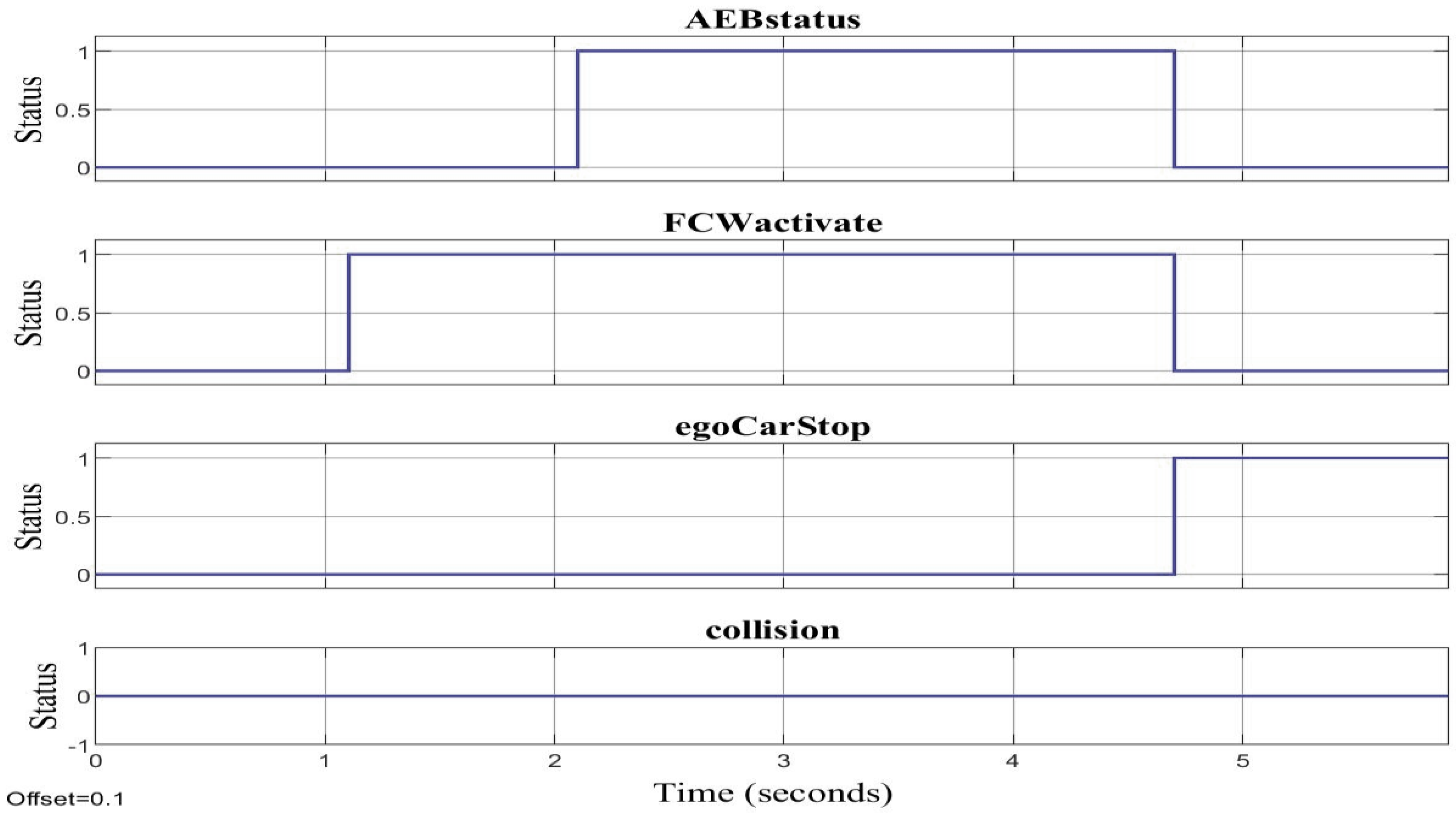
Figure 16 and Figure 17 show how the vehicle’s speed increased and reached its maximum speed of 8.3 m/s in one second, as well as how the FCW and PB influenced the vehicle’s speed. The leading car was identified as soon as the system started, and the ego vehicle used the sensor fusion algorithm to identify it. The first stage of the FCW became true in the 1.2 s condition, at which point the FCW was immediately triggered. After some time when the driver did not apply the brake during the warning period and at 2.2 s, State 2 of the first PB became true, the ego vehicle started to slow down, the first stage of partial braking was engaged, and at 4.7 s, the whole vehicle uniformly stopped. The speed of the ego vehicle is depicted here. The proposed braking system has different reaction times in different scenarios, relative velocities, and relative distances. In the given example scenario, our ego vehicle velocity was 8.33 m/s, the brake was applied at 2.2 s, and the vehicle stopped at 4.7 s. Almost 2.5 s was the reaction time of the first partial braking when the vehicle speed was 8.33 m/s.

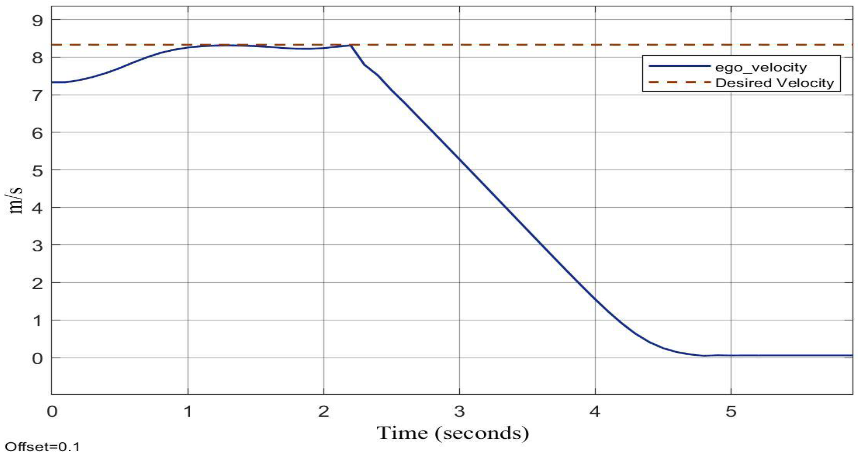
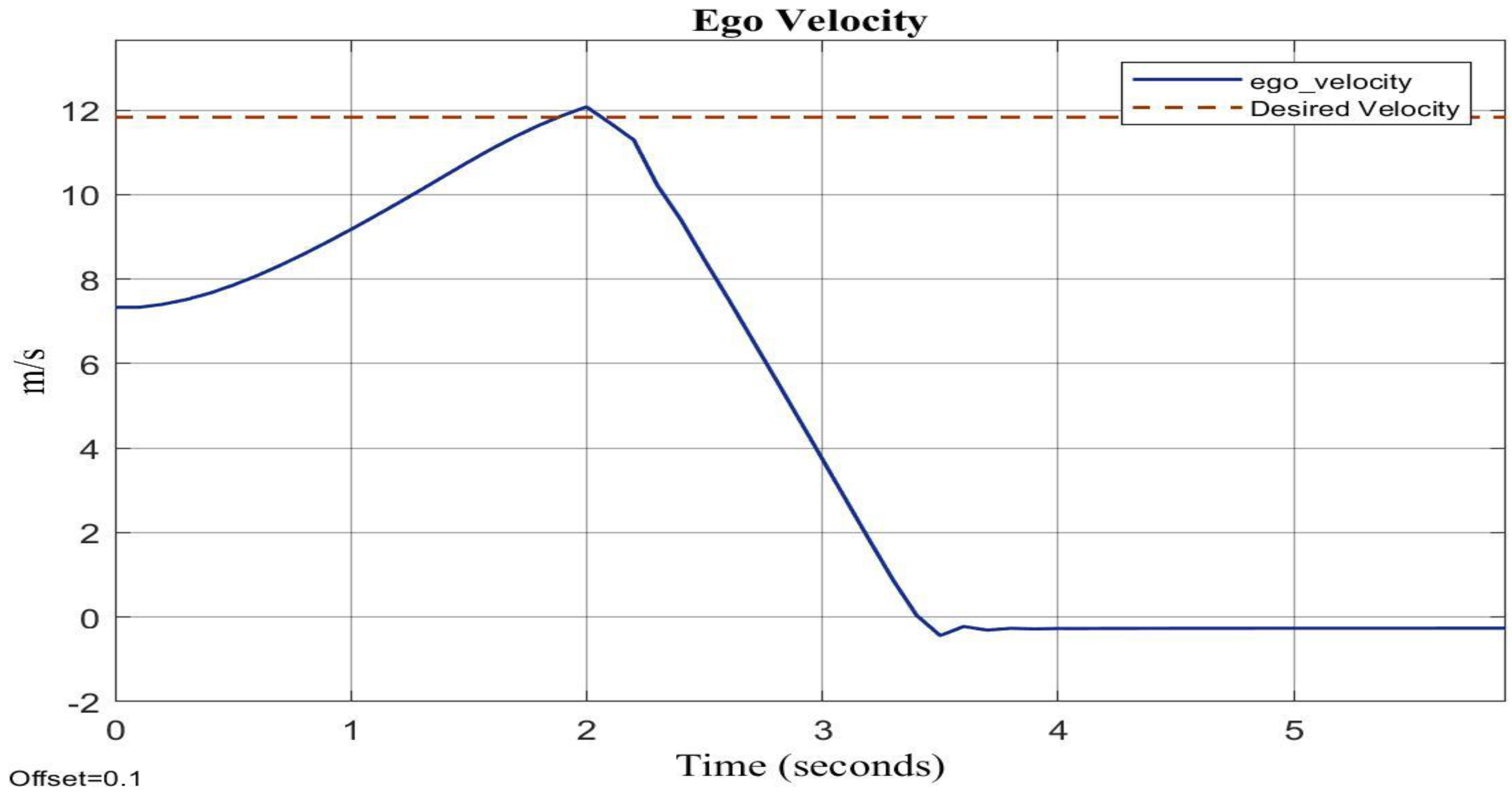
Figure 18 and Figure 19 show how the vehicle’s speed increased until it reached its top speed of 12.33 m/s in 1.8 s. The ego vehicle used the sensor fusion technique to identify the leading vehicle once it was recognized in front after achieving its top speed. In the 1.8 s when the leading vehicle was detected, the first state of the FCW became true and at which point the FCW was immediately triggered. In the next State 2, the first PB became true, the ego vehicle started to slow down, and the first stage of partial braking was engaged. At 2 s, State 3 and the second stage of partial braking occurred and at last, in 2.1 s, State 4 and the fully braking stage were applied. The ego vehicle came to a complete stop at 3.4 s. In this case, the AEB completely avoided the rear end. When the ego vehicle velocity was 12.33 m/s, the brake was applied at 1.8 s and the vehicle stopped at 3.4 s. Almost 1.6 sec was the reaction time. Figure 19 shows the change in vehicle speed as the brakes were applied at various stages.

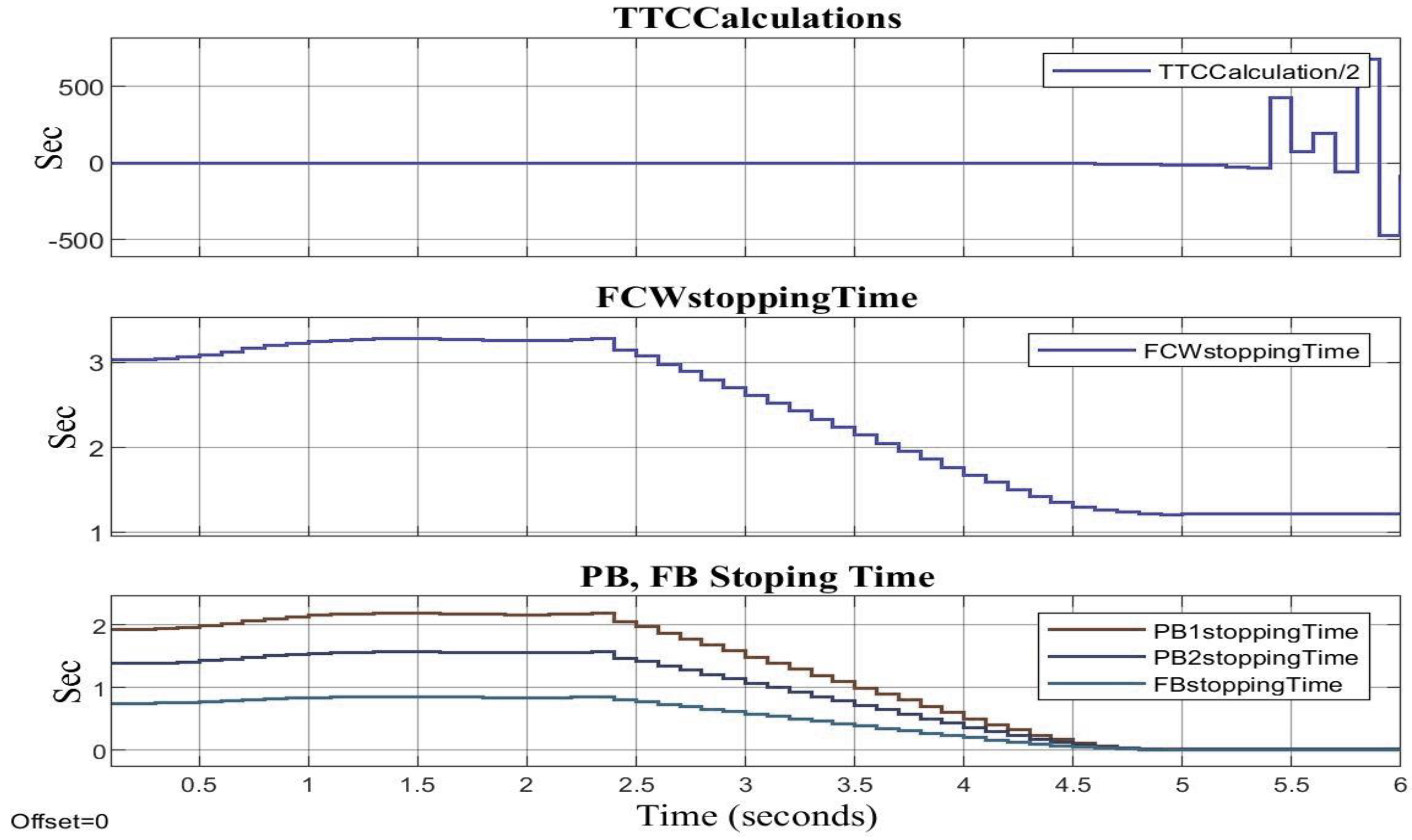
Figure 20 shows the time-to-collision behavior and stop times for the FCW, first and second stage partial braking, and full braking time when the speed of the vehicle changed with time.

6. Comparison with Existing Works

A comparison of the proposed highly efficient AEBS is performed with the existing works in this section. It was seen earlier that the proposed AEBS has increased the reliability and efficiency of the system due to the usage of three kinds of sensors in sensor fusion and non-linear speed controllers.

The proposed AEB system sensor fusion model’s results can be seen. It integrates radars, lidars, and vision to improve the detection accuracy and reliability of the system and that model proposes the model that has a combination of the two different kinds of sensors for fusion.

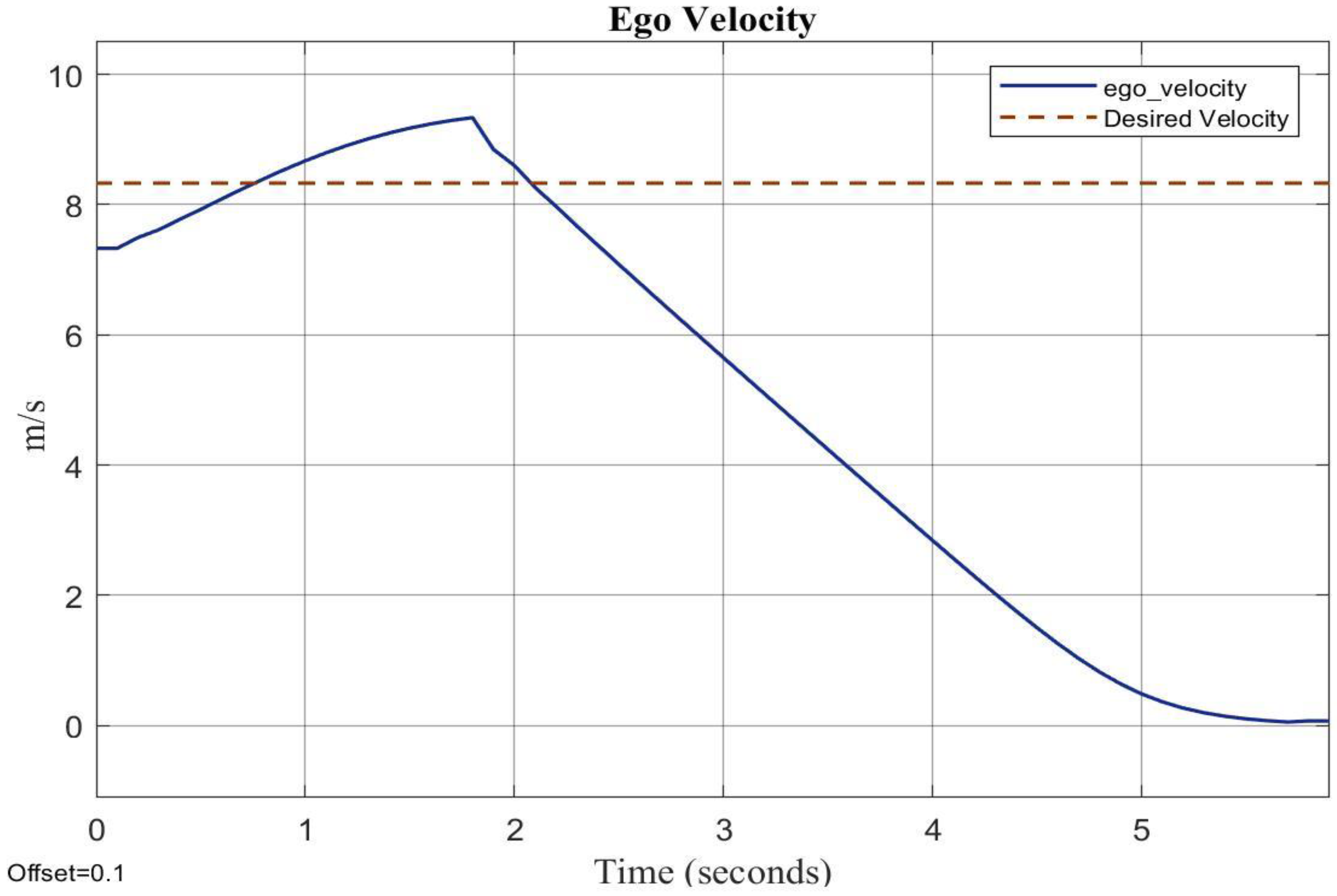
In contrast to earlier linear systems, our advanced system features a non-linear super twisting speed controller. Figure 21 shows how the ego vehicle’s velocity graph behaves when earlier models employ PI as the speed controller. This controller works slowly as the ego vehicle reaches its desired velocity in 1.7 s and takes almost 3.8 s when applying the brake to reach a velocity of zero. As seen from the graph of the velocity in Figure 17, the ST-SMC speed controller takes only 1 s to reach the desired velocity, which means that the settling time is half of that of the previous traditional controller and that the braking time is also less than the previous systems. The proposed AEBS improves the stability and reliability and provides a more accurate and stable output of the fusion model than the earlier approaches. An unstable vehicle detection graph based on noise was produced using prior [34] paper sensor fusion methods. Figure 22 shows the results of the earlier sensor fusion technique when using two sensors. Figure 15 and Figure 22 depict the interactions between the proposed model’s sensor fusion reading and earlier models. A comparison of two previous and advanced models’ fusion of sensors is given in

Table 2. Detail properties of radar, vision, lidar, proposed fusion, and previous fusion.

Properties	Radar	Lidar	Camera	Proposed Fusion	Previous Fusion
Object Detection	Strength	Strength	Capability	Strength	Strength
Pedestrian Detection	Weakness	Capability	Strength	Strength	Capability
Weather Conditions	Strength	Capability	Weakness	Strength	Capability
Lightening Conditions	Strength	Strength	Weakness	Strength	Capability
Dirt	Strength	Capability	Weakness	Strength	Capability
Velocity	Strength	Capability	Capability	Strength	Strength
Distance Accuracy	Capability	Strength	Capability	Strength	Capability
Distance Range	Strength	Capability	Capability	Strength	Strength
Data Density	Weakness	Capability	Strength	Strength	Strength
Classification	Weakness	Capability	Strength	Strength	Capability
Packaging	Strength	Weakness	Capability	Strength	Strength

.

7. Conclusions

To achieve autonomous emergency braking and protect pedestrians, a decision-making algorithm and a dependable sensor fusion architecture were proposed in this paper. The proposed model had three types of sensors: radar, lidar, and vision sensors. The implementation of a simple trajectory prediction and a data-association technique was performed with an emphasis on the effective and trustworthy tracking of various target kinds. To find pedestrians that were either obscured or not spotted, a possible track was used based on a momentary assessment. Track management was provided by the suggested multi-sensor fusion system, which was stable and dependable. Furthermore, the EuroNCAP AEB pedestrian scenarios were thoroughly examined, and suitable collision decision and prediction algorithms were provided. The failure or false positives of any sensor may cause disturbances or accidents; therefore, to obtain an accurate performance of the system, the proposed system managed the trade-off between AEB performance and false positives by setting the threshold for AEB activation and cautiously preventing false positives. This study demonstrated that the suggested AEBS based on sensor fusion is a very reliable option for emergency braking in the autonomous vehicle since it prevented the system from failing in the case of false-positive detection of any one sensor.

To obtain more robust and reliable detection from sensors, advanced fault-tolerant approaches to the sensor fusion part of the system may be used in the future. To increase the system’s accuracy and efficiency, the processing delays caused by the environment may also be considered.