Discriminating Pattern Mining for Diagnosing Reading Disorders ^†

Abstract

Tachistoscopes are devices that display a word for several seconds and ask the user to write down the word. They have been widely employed to increase recognition speed, to increase reading comprehension and, especially, to individuate reading difficulties and disabilities. Once the therapist is provided with the answers of the patients, a challenging problem is the analysis of the strings to individuate common patterns in the erroneous strings that could raise suspicion of related disabilities. In this direction, this work presents a machine learning technique aimed at mining exceptional string patterns and is precisely designed to tackle the above-mentioned problem. The technique is based on non-negative matrix factorization, nnmf, and exploits as features the structure of the words in terms of the letters composing them. To the best of our knowledge, this is the first attempt of mining tachistoscope answers to discover intrinsic peculiarities of the words possibly involved in reading disabilities. From the technical point of view, we present a novel variant of nnmf methods with the adjunctive goal of discriminating between sets. The technique has been experimented in a real case study with the help of an Italian speech therapist center that collaborate with this work.

1. Introduction

Tachistoscopes are widely employed devices useful in many scenarios [1,2,3]. Roughly speaking, these instruments display a word for some milliseconds (on the basis of the wanted difficulty for the exercise) and next the patient is asked for writing down the word. The results shed lights on reading speed, reading comprehension, and are generally helpful to highlight many kinds of reading disorders. Such devices provide the therapist with a set of correctly written words and a set of erroneously written words. Tachistoscopic training, also known as Flash Recognition Training (FRT), in some environments requires that an individual be able to acquire visual information and remember them later on in an optimal way. A second phase requires that the individual express the derived information through verbal, written, or keyboard means. The tachistoscope is therefore used by the speech therapist to evaluate the visual reaction time, speed and recognition interval, automation and visual sequencing. We know that, when a subject with good reading skills is faced with a text, his eyes scan it horizontally line by line and from left to right, in a path defined as “saccades and fixations”. The process, completely automatic, has been known for some time: our eyes proceed “in jumps” of about seven-nine characters, pausing for a few fractions of a second more on some key points generally corresponding to the most important and most significant words. The mechanisms underlying the reading are manifold and integrate with each other. These rapid movements serve to obtain the visual information essential for decoding the text. Among the parameters of the text that influence saccades we include length, lexical frequency, the predictability of words in the text. Proper functioning of attention allows time rapidity for stimulus discrimination, increased sensitivity for the identification of visual stimuli, and a reduction of interferences with close stimuli both in space and in time. This is accomplished by activation of excitatory processes in the predicted spatial region and a decrease of inhibitory processes in unexpected spatial zones [4]. This study that is based on the process of automatic identification of syllables and words is very important for the treatment of reading disorders when there is a deficient development of analysis and visual synthesis processes but which must be combined with specific work on neuropsychological aspects such as visual attention and the phonological loop [5]. The methods of presentation are: (i) stimulus, preceded by the “alert” in the central position, ($ii$) appearance of the stimulus in random positions so as to also influence the speed of attention shift. The aim is to achieve an adequate speed level by changing the stimulus exposure time. Several studies concerning the fluidity of reading have underlined and explained the importance of the speed and effectiveness of the shift of attention [6,7,8,9]. The proposals, therefore, are divided into several phases: recognition of the distinctive features of the letters widening the focus of recognition from the syllable, to the morpheme, to the word rapid shift of attention to normalization of eye movements (saccades). The reading of words with tachistoscopic mode is used by gradually decreasing the exposure time of the word—first in a central position and then in random positions—starting with simple bisyllabic words and then proceeding with increasingly complex words up to the trisyllabic quadrisyllabic words with double and a consonant cluster.

Computer science contribution for speech disorders is witnessing a great interest [10,11,12,13] and, to the best to our knowledge, this is the first work trying to help therapists which employ tachistoscopes in diagnosing by automatically collecting and analysing information.

A challenging problem from a computer science point of view is that of suggesting characteristics of the words that discriminate, for a patient, between correct and erroneous answer, namely, characteristics shared by erroneously answered words and low-frequently present in the set of correctly answered words. We address the problem by borrowing the results on non-negative matrix factorization [14,15,16], a widely employed basic technique able to decompose an input matrix into two lower rank matrices. This method has been successful for the extraction of concepts/topics from unstructured text [17], for speak verification [18], for feature extraction, for clustering, for classification and many other fields [19].

The technique analyzes outcomes of tachistoscope sessions by firstly vectorizing words and secondly extracting prototype of errors. For this second part, nnmf is exploited, and its objective function is relevantly changed to allow us to achieve two purposes, approximating input vectors and discriminating the correctness. Furthermore, contexts are analyzed to provide indications about problematic scenarios and, equipped with the information of encoded pathologies, the framework is able to suggest the presence of known diseases or of not yet structured ones.

The work provides then a contribution in the following aspects (i) to the best of our knowledge; this is the first attempt to automatically diagnose reading pathologies starting by tachistoscope output ($ii$) a nonnegative matrix factorization technique able to take simultaneously into account two sets of words is provided; ($iii$) an ad-hoc discrimination power is embedded in the formulation of the nnmf problem; ($iv$) the analysis of the contexts potentially influencing disorders is performed as a phase of the technique; (v) the system is able to individuate an already encoded pathology and/or unencoded ones.

The paper is organized as follows: Section 2 reports the notation employed throughout the paper and preliminary notions; Section 3 describes the proposed technique; and Section 4 illustrates the experimental campaign conducted on both real and synthetic data. Finally, Section 5 depicts conclusions.

2. Preliminaries

In this section, we present the tachistoscope, the data coming from it, and introduce preliminary concepts about features and methodology goals.

2.1. Tachistoscope

Tachistoscopes are widely employed devices useful in many scenarios [1,20]. Roughly speaking, these instruments display a word for some milliseconds (on the basis of the wanted difficulty for the exercise) and next the patient is asked for writing down the word. The results shed lights on reading speed, reading comprehension and are generally helpful to highlight many kinds of reading disorders. Such devices provide the therapist with a set of correctly written words and a set of erroneously written words. Tachistoscopic training, also known as Flash Recognition Training (FRT) in some environments, requires that an individual be able to acquire visual information and remember them later on in an optimal way. A second phase requires that the individual express the derived information through verbal, written, or keyboard means. The tachistoscope is therefore used by the speech therapist to evaluate the visual reaction time, speed and recognition interval, automation and visual sequencing.

In a session, the user is provided with a sequence of trials each having a word associated with it. The trial consists of two phases: visualization phase and guessing phase. During the visualization phase, a word is shown for some milliseconds (typically ranging from 15 to 1500). To this phase, the guessing phase follows. During this phase, the word disappears and the user has to guess the word by typing it. After that, the word disappears; it could be substituted by a set of ‘#’ to increase the difficulty since the user loses the visual memory. In such a case, the word is said “masked”.

The therapist, other than the visualization time, can impose several settings about the word—in particular, (i) the frequency of the word, which represents how much the word is in current use; ($ii$) the length of the word, which represents how long the word is; ($iii$) the easiness of the word, which represents how difficult reading and writing the word is (for example, each consonant is followed by a vowel); ($iv$) the existence of the word, which represents the existence of the word in the dictionary. As for the existence of the word, the tachistoscope is able to show both existing words and non-existing words which are random sequences of letters with the constraints that (i) each syllable has to appear in at least one existing word and (ii) each pair of adjacent letters has to appear in at least one existing word. The constraints aim at generating readable sequences of letters.

2.2. Encoded Pathologies

Literature on speech disorders reports some studies about the frequent error patterns for some pathologies. We can, then, encode these pathologies in the rows of a matrix $\mathrm{Y}$ where the columns are associated with the features discussed in the following section.

2.3. Input Data, Feature Extraction

The data under analysis, as provided by tachistoscope, consist of a set of word split in two subsets: (i) the set of words with correct answers and ($ii$) the set with incorrect answers. On these data, two families of features can be highlighted: structural features and contextual features. Nevertheless, note that the proposed framework is extensible to other sets of features without changes to the technical building.

2.3.1. Structural Features

The structural features encode the characteristics of the associated word and there are two groups: alphabet letters and letter pairs. Note that, by construction, not all the letter pairs are taken into account but just the pairs of adjacent letters appearing in existing or non-existing words. In the following, we often call “valid” these pairs of letters. In addition, a third group of structural features is taken into account. Features in this group are related to known letter/letter pairs errors in encoded pathologies. For example, when dyslexia is related to spatial errors, namely confusion of graphemes with similar spatial parameters, classical errors are p erroneously reported as b or as q by the effect of rotation or overturn of the read letter.

2.3.2. Contextual Features

The contextual features encode the characteristics of the scenario related to the answer: time, masking, existence, length, frequency, easiness.

The two sets of features have relevance in different phases and are utilized in different ways. Indeed, for domain experts, the context features are not very interesting for their discriminative power; indeed, their effect on the capability of guessing the correct answer is quite obvious. For example, the lower the visualization time, the lower is the probability of providing correct answers, or the higher the difficulty of the word, the lower is the probability of providing correct answers, and so on.

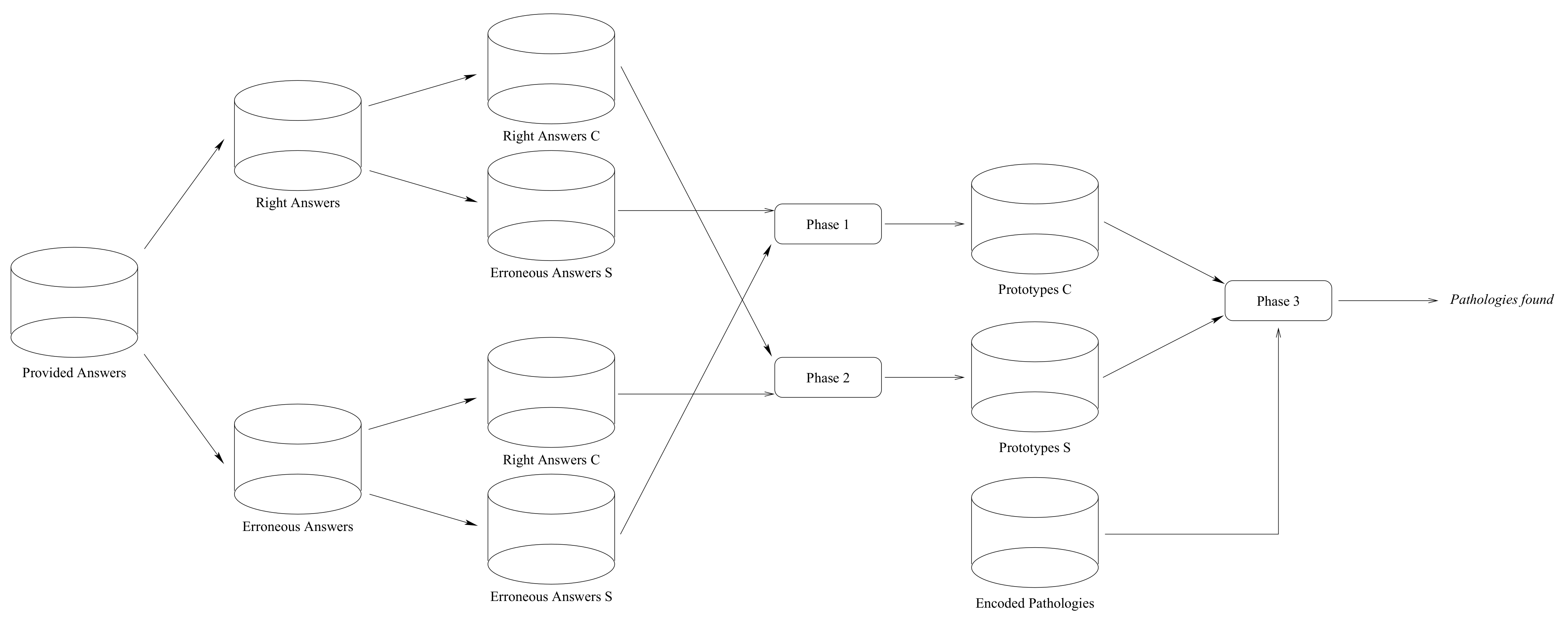
2.3.3. Phases of the Method

The proposed framework is a three phases learning system, sketched in Figure 1.

• Phase 1: Discriminating Pattern Search

The first phase aims at discovering prototypes, namely special words encoding those peculiarities of the words representing the main obstacles for the user; a bit more formally, we look for features that are representative of the set of words associated with correct answers and not representative of the set of words associated with incorrect answers.

• Phase 2: Context Analysis

The second phase aims at deep examination of the context associated with the prototypes. This phase is devoted at evaluating which context features are the most influential cause of providing the wrong answer. Thus, the behavior of the context feature on the prototypes is analyzed.

• Phase 3: Encoded Pathology Detection

The third phase aims at individuating which encoded pathologies are disguised in the data. In particular, for some pathologies, the most frequent related errors are known. Thus, the goal is to find error patterns shared between data and pathologies and the level of the matching for indicating to the expert which pathologies are expressed and how much they affect the patient answers.

3. Technique

3.1. Preliminaries

In this section, the main notation employed throughout the paper is presented.

$\mathsf{\Sigma }$ denotes the reference alphabet and each element of $\mathsf{\Sigma }$ is also denoted as letter; for example, $\mathsf{\Sigma }$ could be composed by the 26 letters of the English alphabet. A word is an ordered finite sequence of element of $\mathsf{\Sigma }$, namely an element of ${\mathsf{\Sigma }}^{*}$. A tachistoscope session $\mathcal{S}$ consists of the subministration of a set of words to the user under analysis, with the same contextual configuration, namely the same values of time, masking, existence, length, frequency, and easiness. From each tachistoscope session, the set of user answers is collected. Let $\mathbf{S}$ denote the set of all the tachistoscope sessions.

$\mathsf{\Lambda }=\{‘\mathit{right} \mathit{answer}’,‘\mathit{erroneous} \mathit{answer}’\}$ denotes a set of labels and $\lambda :{\mathsf{\Sigma }}^{*}\times \mathbf{S}\to \Lambda$ denotes the labeling function that associates a word from a set of words $\mathbf{W}$ with a label from $\mathsf{\Lambda }$ on the basis of user results coming from the tachistoscope during the session $\mathcal{S}\in \mathbf{S}$, where $\mathbf{W}$ has been subministrated. A test $\mathbf{T}=\{{\mathcal{S}}_1,\dots ,{\mathcal{S}}_k\}\subseteq \mathbf{S}$ is the set of all the tachistoscope sessions subministered to the same user under analysis. A multiset of words ${\mathbf{W}}_{\mathbf{T}}$ is associated with $\mathbf{T}$ obtained by putting together the set of words ${\mathbf{W}}_{{\mathcal{S}}_1},\dots ,{\mathbf{W}}_{{\mathcal{S}}_k}$ associated with sessions ${\mathcal{S}}_1,\dots ,{\mathcal{S}}_k$.

3.1.1. Session Vectorization

Let $\mathcal{S}$ be a tachistoscope session and let $\mathbf{W}\subseteq {\mathsf{\Sigma }}^{*}$ be the set of words associated with $\mathcal{S}$. $\mathbf{W}$ is semantically split into two subsets:

• the set of words with right answers ${\mathbf{W}}_r=\{w\in \mathbf{W}\mathit{s}.\mathit{t}.\lambda \left(w\right)=‘\mathit{right} \mathit{answer}’\}$;
• the set of words with erroneous answers ${\mathbf{W}}_e=\{w\in \mathbf{W}\mathit{s}.\mathit{t}.\lambda \left(w\right)=‘\mathit{erroneous} \mathit{answer}’\}$.

Each word $w\in \mathbf{W}$ is transformed in a $n_f$-dimensional vector $v_w$ by mapping w from the space associated with ${\mathsf{\Sigma }}^{*}$ on a feature space $\mathcal{F}$ having size $n_f$. The considered feature space consists of two subsets ${\mathcal{F}}_c$ and ${\mathcal{F}}_s$, described below.

3.1.2. Contextual Features

${\mathcal{F}}_c$ represents the set of contextual features, and it is composed of six elements detailed next together with the associated domain:

time: 

the time in milliseconds of the trial associated with w;

masking: 

a binary value stating whether the “masking” is active or not;

existence: 

a binary value stating whether the word is in the dictionary or not;

length: 

the number of characters of the word;

frequency: 

a binary value stating whether the word is of common use or not;

easiness: 

a binary value stating whether the structure of the word is simple.

3.1.3. Structural Features

${\mathcal{F}}_s$ represents the set of structural features, and it is composed by $\left|\mathsf{\Sigma }\right|$ attributes, one for each alphabet letter, plus $n_p\ll {\left|\mathsf{\Sigma }\right|}^2$ attributes, one for each valid pair of adjacent letters, where valid is referred to the used language, namely a word is valid if exists at least one word in the considered language vocabulary $\mathbf{W}$ containing such a pair. Note that the features in ${\mathcal{F}}_c$ depend only on the session $\mathcal{S}$, while the features in ${\mathcal{F}}_s$ depend on the word. Thus, all the vectors related to the set of words associated with the same sessions assume the same value on the set of features ${\mathcal{F}}_c$. Moreover, note that, since ${\mathcal{F}}_s$ contains only valid pairs and since the concept of valid strictly depends on the set of input words, the set of feature $\mathcal{F}$ is a function of the set of words. However, for each session, administrated words are randomly picked from a fixed set of words hard coded into the tachistoscope system. Thus, ${\mathcal{F}}_s$ can be also be generated by considering all the words included in the system.

3.1.4. Test Vectorization

Let $\mathbf{T}=\{{\mathcal{S}}_1,\dots ,{\mathcal{S}}_k\}$ be a test and $\mathcal{F}$ be the set of features. A dataset $\mathbf{DS}$ in $n\times \left|\mathcal{F}\right|$ matrix form is associated with $\mathbf{T}$ by mapping for each session $\mathcal{S}\in \mathbf{T}$, each word $w\in \mathcal{S}$ in a vector $v_w$. The dataset $\mathbf{DS}$ is semantically split into two datasets ${\mathbf{DS}}_e$ and ${\mathbf{DS}}_r$, the former associated with the set of words ${\mathbf{W}}_r$ and the latter associated with the set of words ${\mathbf{W}}_e$.

Each datasets is, in turn, vertically split into two datasets, ${\mathbf{DS}}_{*}^s$ and ${\mathbf{DS}}_{*}^c$, the former associated with structural features and the latter associated with the contextual features; thus, there are four datasets ${\mathbf{DS}}_e^s$, ${\mathbf{DS}}_e^c$, ${\mathbf{DS}}_r^s$ and ${\mathbf{DS}}_r^s$.

As for the dataset building, an entry $\mathbf{DS}(i,·)$ in $\mathbf{DS}$ is associated with each word $w_i$ in $\mathbf{W}$ and, in particular, $\mathbf{DS}(i,j)$ represents the value that $w_i$ assumes on the feature ${\mathcal{F}}_i$. For a structural feature f, the value assumed by a word w on f is the number of times the letter or the pair of letters associated with f occurs in w. Conversely, for the contextual features, the value assumed by a word w on them is that previously listed.

3.2. Phase 1: Discriminating Prototype Search

In this phase, we consider only matrices ${\mathbf{DS}}_e^s$ and ${\mathbf{DS}}_r^s$ since the goal is the mining of peculiarities in the structure of the words able to discriminate between ${\mathbf{W}}_e$ and ${\mathbf{W}}_r$ and since the contextual features are already expected to be discriminative. Moreover, the contextual features could affect the results since they hide difficulties of the user in structural component of the words.

The idea of the approach exploits a non-negative matrix factorization technique and an innovative optimization objective precisely designed for the situation at hand. The aim is to decompose matrix ${\mathbf{DS}}_e^s$ having size $n_e\times m$ into two less-ranked matrices ${\mathsf{\Theta }}_e$ (having size $n_e\times n_p$) and ${\mathcal{P}}_e^s$ (having size $n_p\times m$). Here, ${\mathcal{P}}_e^s$ represents the $n_p$ prototype words, and ${\mathsf{\Theta }}_e$ represents the impact of each word in ${\mathbf{W}}_e$ for the emerging of each prototype. Analogously, ${\mathbf{DS}}_r^s$ should be decomposed as ${\mathsf{\Theta }}_r·{\mathcal{P}}_r^s$. In order to find matrices ${\mathsf{\Theta }}_e$, ${\mathcal{P}}_e^s$, ${\mathsf{\Theta }}_r$ and ${\mathcal{P}}_r^s$, we have to keep in mind three desiderata:

• ${\mathbf{DS}}_e^s\approx {\mathsf{\Theta }}_e·{\mathcal{P}}_e^s$;
• ${\mathbf{DS}}_r^s\approx {\mathsf{\Theta }}_r·{\mathcal{P}}_r^s$;
• the prototype words should be able to discriminate between ${\mathbf{W}}_e$ and ${\mathbf{W}}_r$.

To achieve the third goal, the sets of prototypes in ${\mathcal{P}}_e^s$ and in ${\mathcal{P}}_r^s$ should be as much different as possible. Thus, for handling the goals, given matrices ${\mathbf{DS}}_e$ and ${\mathbf{DS}}_r$, we aim at finding matrices ${\mathsf{\Theta }}_e$, ${\mathcal{P}}_e^s$, ${\mathsf{\Theta }}_r$ and ${\mathcal{P}}_r^s$ such that the function

$$\begin{array}{c}\hfill {\varphi }_s({\mathsf{\Theta }}_e,{\mathcal{P}}_e^s,{\mathsf{\Theta }}_r,{\mathcal{P}}_r^s)=\frac{1}{2n_e}{∥{\mathbf{DS}}_e^s-{\mathsf{\Theta }}_e·{\mathcal{P}}_e^s∥}_F^2+\frac{1}{2n_r}{∥{\mathbf{DS}}_r^s-{\mathsf{\Theta }}_r·{\mathcal{P}}_r^s∥}_F^2-\gamma ({\mathcal{P}}_e^s,{\mathcal{P}}_r^s)\end{array}$$

(1)

is minimized, where ${\parallel ·\parallel }_F^2$ represents the Frobenius norm and $\gamma (·,·)$ is the discriminating power between ${\mathcal{P}}_e^s$ and ${\mathcal{P}}_r^s$, as defined in the next section.

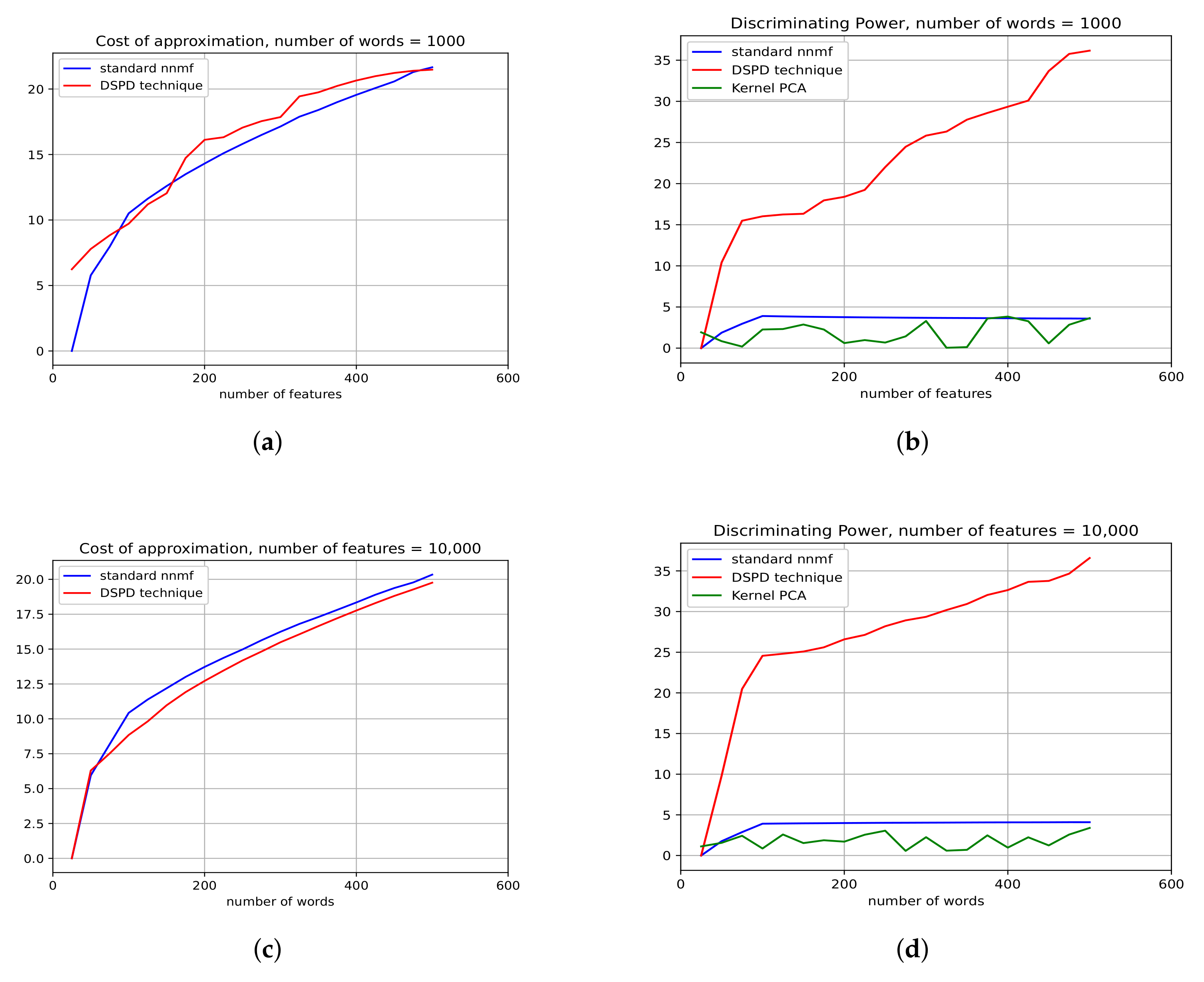
3.2.1. Discriminating Power

The discriminating power of prototypes ${\mathcal{P}}_e^s$ and ${\mathcal{P}}_r^s$ is defined with the aim of measuring their ability in discriminating between populations ${\mathbf{W}}_e$ and ${\mathbf{W}}_r$ and, simultaneously, of keeping ${\mathcal{P}}_e^s$ and ${\mathcal{P}}_r^s$ as good representatives, respectively, of ${\mathbf{W}}_e$ and ${\mathbf{W}}_r$.

With this idea in mind, we build a discriminating power that computes all pairs of distances between each prototype word in ${\mathcal{P}}_e^s$ (resp. ${\mathcal{P}}_r^s$) and the aim is that of minimizing the sum of such distances.

In order to guide the optimization process in not magnifying feature not occurring in the input sets to improve the discrimination power, we weight prototypes matrices for the support of each feature in the input set, where the support of a feature is the number of words in the input set matching the features.

Definition 1

(Support). Given a dataset $\mathbf{DS}$ having size $n\times m$ and a set of structural features $\mathcal{F}$, thesupportσ of $\mathcal{F}$ in $\mathbf{DS}$ is a m-sized vector where $\sigma \left(i\right)={\sum }_j\mathbf{DS}(i,j)$. The support matrix σ is an $m\times m$ matrix having the elements of σ along the main diagonal and 0 elsewhere.

In order to compute the discriminating power, we need to introduce two transformation matrices. Let $n_p\times m$ be the dimension of ${\mathcal{P}}_e^s$ and ${\mathcal{P}}_r^s$ having by construction the same dimension. Firstly, consider the matrix $\mathbf{I}\left(n_p\right)$ defined as

$$\mathbf{I}\left(n_p\right)={({\mathbf{U}}_{n_p}^0,\dots ,{\mathbf{U}}_{n_p}^{n_p-1})}^T$$

where ${\mathbf{U}}_{n_p}^i$ is a $n_p\times n_p$ matrix having ones on column i and zero elsewhere and ${·}^T$ represents the transpose. Secondly, consider the matrix $\mathbf{J}\left(n_p\right)$ defined as

$$\mathbf{J}\left(n_p\right)={(\underset{n_p}{\underbrace{{\Delta }_{n_p},\dots ,{\Delta }_{n_p}}})}^T$$

where ${\Delta }_{n_p}$ is the $n_p\times n_p$ identity matrix.

Definition 2

(Discriminating power). Given two prototype matrices ${\mathcal{P}}_e^s$ and ${\mathcal{P}}_r^s$, the discriminating power is defined as

$$\gamma ({\mathcal{P}}_e^s,{\mathcal{P}}_r^s)={∥\mathbf{I}\left(n_p\right)·{\mathcal{P}}_e^s·{\sigma }_e-\mathbf{J}\left(k\right)·{\mathcal{P}}_r^s·{\sigma }_r∥}_F^2.$$

This function accounts for all pairs of distances between prototypes in ${\mathcal{P}}_e^s$ and prototypes in ${\mathcal{P}}_r^s$. Thus, the higher $\gamma ({\mathcal{P}}_e^s,{\mathcal{P}}_r^s)$ is, the higher is the discriminating power.

3.2.2. Computational Issues

In order to solve the optimization problem consisting of minimizing the function ${\varphi }_s$ depicted in (1), we adopt the gradient descent algorithm where variables ${\mathcal{P}}_e^s$, ${\mathcal{P}}_r^s$, ${\mathsf{\Theta }}_e$ and ${\mathsf{\Theta }}_r$ are updated by calculating the gradient of f and projecting the update on the non-negative orthant ${\mathbb{R}}_{+}^n$. Thus, we have:

$$\left\{\begin{array}{c}{\mathcal{P}}_r^{s(k+1)}={\mathcal{P}}_r^{s\left(k\right)}-\nabla {\varphi }_s\left({\mathsf{\Theta }}_e^{\left(k\right)},{\mathcal{P}}_e^{s\left(k\right)},{\mathsf{\Theta }}_r^{\left(k\right)},{\mathcal{P}}_r^{s\left(k\right)}\right)\hfill \\ {\mathcal{P}}_e^{s(k+1)}={\mathcal{P}}_e^{s\left(k\right)}-\nabla {\varphi }_s\left({\mathsf{\Theta }}_e^{\left(k\right)},{\mathcal{P}}_e^{s\left(k\right)},{\mathsf{\Theta }}_r^{\left(k\right)},{\mathcal{P}}_r^{s\left(k\right)}\right)\hfill \\ {\mathsf{\Theta }}_r^{(k+1)}={\mathsf{\Theta }}_r^{\left(k\right)}-\nabla {\varphi }_s\left({\mathsf{\Theta }}_e^{\left(k\right)},{\mathcal{P}}_e^{s\left(k\right)},{\mathsf{\Theta }}_r^{\left(k\right)},{\mathcal{P}}_r^{s\left(k\right)}\right)\hfill \\ {\mathsf{\Theta }}_e^{(k+1)}={\mathsf{\Theta }}_e^{\left(k\right)}-\nabla {\varphi }_s\left({\mathsf{\Theta }}_e^{\left(k\right)},{\mathcal{P}}_e^{s\left(k\right)},{\mathsf{\Theta }}_r^{\left(k\right)},{\mathcal{P}}_r^{s\left(k\right)}\right)\hfill \end{array}\right.$$

(2)

where ${·}^{\left(k\right)}$ indicates the matrix computed at the k-th iteration. In the following part of the section, we report details only about the update of ${\mathsf{\Theta }}_e$ and ${\mathcal{P}}_e^s$ since the computation of the update of ${\mathsf{\Theta }}_r$ and ${\mathcal{P}}_r^s$ follows the same line of reasoning.

Recall on Trace Derivative Computation

Preliminarily, recall that, given matrices $\mathbf{X}$, $\mathbf{Y}$, $\mathbf{H}$ and $\mathbf{T}$, it holds that:

$$\begin{array}{c}\hfill \frac{\partial tr\left[\mathbf{X}\mathbf{H}\mathbf{Y}\right]}{\partial \mathbf{H}}={\mathbf{X}}^T{\mathbf{Y}}^T,\frac{\partial tr\left[\mathbf{X}{\mathbf{H}}^T\mathbf{Y}\right]}{\partial \mathbf{H}}=\mathbf{Y}\mathbf{X},\end{array}$$

where $tr(·)$ denotes the trace, and that

$$\begin{array}{cc}\hfill {∥\mathbf{X}-\mathbf{Y}\mathbf{H}∥}_F^2=& tr\left[\left(\mathbf{X}-\mathbf{Y}\mathbf{H}\right){(\mathbf{X}-\mathbf{Y}\mathbf{H})}^T\right]=tr\left[\mathbf{X}{\mathbf{X}}^T\right]-tr\left[\mathbf{X}{\mathbf{H}}^T{\mathbf{Y}}^T\right]-tr\left[\mathbf{Y}\mathbf{H}{\mathbf{X}}^T\right]+tr\left[\mathbf{Y}\mathbf{H}{\mathbf{H}}^T{\mathbf{Y}}^T\right].\hfill \end{array}$$

Thus

$$\begin{array}{cc}\hfill \frac{\partial {∥\mathbf{X}-\mathbf{Y}\mathbf{H}∥}_F^2}{\partial \mathbf{Y}}=& \frac{\partial tr\left[\mathbf{X}{\mathbf{X}}^T\right]}{\partial \mathbf{Y}}-\frac{\partial tr\left[\mathbf{X}{\mathbf{H}}^T{\mathbf{Y}}^T\right]}{\partial \mathbf{Y}}-\frac{\partial tr\left[\mathbf{Y}\mathbf{H}{\mathbf{X}}^T\right]}{\partial \mathbf{Y}}+\frac{\partial tr\left[\mathbf{Y}\mathbf{H}{\mathbf{H}}^T{\mathbf{Y}}^T\right]}{\partial \mathbf{Y}}\hfill \\ \hfill =& 0-\mathbf{X}{\mathbf{H}}^T-\mathbf{X}{\mathbf{H}}^T+\frac{\partial \mathbf{Y}\mathbf{A}}{\partial \mathbf{Y}}+\frac{\partial \mathbf{B}{\mathbf{Y}}^T}{\partial \mathbf{Y}}\hfill \end{array}$$

with $\mathbf{A}=\mathbf{H}{\mathbf{H}}^T{\mathbf{Y}}^T$ and $\mathbf{B}=\mathbf{Y}\mathbf{H}{\mathbf{H}}^T$, consequently

$$\begin{array}{cc}\hfill \frac{\partial {∥\mathbf{X}-\mathbf{Y}\mathbf{H}∥}_F^2}{\partial \mathbf{Y}}=& -2\mathbf{X}{\mathbf{H}}^T+{\mathbf{A}}^T+\mathbf{B}=-2\mathbf{X}{\mathbf{H}}^T+2\mathbf{Y}\mathbf{H}{\mathbf{H}}^T=-2\left(\mathbf{X}-\mathbf{Y}\mathbf{H}\right){\mathbf{H}}^T.\hfill \end{array}$$

Analogously

$$\begin{array}{cc}\hfill \frac{\partial {∥\mathbf{X}-\mathbf{Y}\mathbf{H}∥}_F^2}{\partial \mathbf{H}}=& \frac{\partial tr\left[\mathbf{X}{\mathbf{X}}^T\right]}{\partial \mathbf{H}}-\frac{\partial tr\left[\mathbf{X}{\mathbf{H}}^T{\mathbf{Y}}^T\right]}{\partial \mathbf{H}}-\frac{\partial tr\left[\mathbf{Y}\mathbf{H}{\mathbf{X}}^T\right]}{\partial \mathbf{H}}+\frac{\partial tr\left[\mathbf{Y}\mathbf{H}{\mathbf{H}}^T{\mathbf{Y}}^T\right]}{\partial \mathbf{H}}\hfill \\ \hfill =& 0-{\mathbf{Y}}^T\mathbf{X}-{\mathbf{Y}}^T\mathbf{X}+\frac{\partial \mathbf{Y}\mathbf{H}\mathbf{A}}{\partial \mathbf{H}}+\frac{\partial \mathbf{B}{\mathbf{H}}^T{\mathbf{Y}}^T}{\partial \mathbf{H}}\hfill \end{array}$$

with $\mathbf{A}={\mathbf{H}}^T{\mathbf{Y}}^T$ and $\mathbf{B}=\mathbf{Y}\mathbf{H}$, consequently

$$\begin{array}{cc}\hfill \frac{\partial {∥\mathbf{X}-\mathbf{Y}\mathbf{H}∥}_F^2}{\partial \mathbf{H}}=& -2{\mathbf{Y}}^T\mathbf{X}+{\mathbf{Y}}^T{\mathbf{A}}^T+{\mathbf{Y}}^T\mathbf{B}=-2{\mathbf{Y}}^T\mathbf{X}+{\mathbf{Y}}^T\mathbf{Y}\mathbf{H}+{\mathbf{Y}}^T\mathbf{Y}\mathbf{H}\hfill \\ \hfill =& -2{\mathbf{Y}}^T\mathbf{X}+2{\mathbf{Y}}^T\mathbf{Y}\mathbf{H}=-2{\mathbf{Y}}^T\left(\mathbf{X}-\mathbf{Y}\mathbf{H}\right).\hfill \end{array}$$

Finally

$$\begin{array}{cc}\hfill \frac{\partial {∥\mathbf{Y}\mathbf{X}\mathbf{H}-\mathbf{T}∥}_F^2}{\partial \mathbf{X}}=& \frac{\partial tr\left[\mathbf{Y}\mathbf{X}\mathbf{H}{\left(\mathbf{Y}\mathbf{X}\mathbf{H}\right)}^T\right]}{\partial \mathbf{X}}-\frac{\partial tr\left[\mathbf{Y}\mathbf{X}\mathbf{H}{\mathbf{T}}^T\right]}{\partial \mathbf{X}}-\frac{\partial tr\left[\mathbf{T}{\left(\mathbf{Y}\mathbf{X}\mathbf{H}\right)}^T\right]}{\partial \mathbf{X}}+\frac{\partial tr\left[\mathbf{T}{\mathbf{T}}^T\right]}{\partial \mathbf{X}}\hfill \\ \hfill =& \frac{\partial tr\left[\mathbf{Y}\mathbf{X}\mathbf{H}{\mathbf{H}}^T{\mathbf{X}}^T{\mathbf{Y}}^{\mathbf{T}}\right]}{\partial \mathbf{X}}-\frac{\partial tr\left[\mathbf{Y}\mathbf{X}\mathbf{H}{\mathbf{T}}^T\right]}{\partial \mathbf{X}}-\frac{\partial tr\left[\mathbf{T}{\mathbf{H}}^T{\mathbf{X}}^T{\mathbf{Y}}^T\right]}{\partial \mathbf{X}}+0\hfill \\ \hfill =& \frac{\partial tr\left[\mathbf{Y}\mathbf{X}\mathbf{A}\right]}{\partial \mathbf{X}}+\frac{\partial tr\left[\mathbf{B}{\mathbf{X}}^T{\mathbf{Y}}^{\mathbf{T}}\right]}{\partial \mathbf{X}}-{\mathbf{Y}}^T\mathbf{T}{\mathbf{H}}^T-{\mathbf{Y}}^T\mathbf{T}{\mathbf{H}}^T\hfill \end{array}$$

with $\mathbf{A}=\mathbf{H}{\mathbf{H}}^T{\mathbf{X}}^T{\mathbf{Y}}^{\mathbf{T}}$ and $\mathbf{B}=\mathbf{Y}\mathbf{X}\mathbf{H}{\mathbf{H}}^T$, consequently

$$\begin{array}{cc}\hfill \frac{\partial {∥\mathbf{Y}\mathbf{X}\mathbf{H}-\mathbf{T}∥}_F^2}{\partial \mathbf{X}}=& {\mathbf{Y}}^T{\mathbf{A}}^T+{\mathbf{Y}}^T\mathbf{B}-2{\mathbf{Y}}^T\mathbf{T}{\mathbf{H}}^T={\mathbf{Y}}^T\mathbf{Y}\mathbf{X}\mathbf{H}{\mathbf{H}}^T+{\mathbf{Y}}^T\mathbf{Y}\mathbf{X}\mathbf{H}{\mathbf{H}}^T-2{\mathbf{Y}}^T\mathbf{T}{\mathbf{H}}^T\hfill \\ \hfill =& 2{\mathbf{Y}}^T\mathbf{Y}\mathbf{X}\mathbf{H}{\mathbf{H}}^T-2{\mathbf{Y}}^T\mathbf{T}{\mathbf{H}}^T=2{\mathbf{Y}}^T\left(\mathbf{Y}\mathbf{X}\mathbf{H}-\mathbf{T}\right){\mathbf{H}}^T.\hfill \end{array}$$

As for the computation of ${\mathsf{\Theta }}_e$, the gradient of ${\varphi }_s$ has to be computed relatively to ${\mathsf{\Theta }}_e$ and, then, since both $\frac{1}{2n_r}{∥{\mathbf{DS}}_r^s-{\mathsf{\Theta }}_r·{\mathcal{P}}_r^s∥}_F^2$ and $\gamma ({\mathcal{P}}_e^s,{\mathcal{P}}_r^s)$ do not depend on ${\mathsf{\Theta }}_e$, it follows that

$$\begin{array}{cc}\hfill \frac{\partial {\varphi }_s}{\partial {\mathsf{\Theta }}_e}& =\frac{1}{2n_e}\frac{\partial }{\partial {\mathsf{\Theta }}_e}\left(\parallel {\mathbf{DS}}_e-{\mathsf{\Theta }}_e·{\mathcal{P}}_e^s{\parallel }_F^2\right)=\frac{1}{2n_e}\left(-2\left({\mathbf{DS}}_e-{\mathsf{\Theta }}_e·{\mathcal{P}}_e^s\right)·{\mathcal{P}}_e^{sT}\right)\hfill \\ \hfill & =-\frac{1}{n_e}\left({\mathbf{DS}}_e-{\mathsf{\Theta }}_e·{\mathcal{P}}_e^s\right)·{\mathcal{P}}_e^{sT}.\hfill \end{array}$$

Conversely, as for the computation of ${\mathcal{P}}_e^s$, the gradient of ${\varphi }_s$ has to be computed relatively to ${\mathcal{P}}_e^s$ and, then, since $\frac{1}{2n_r}{∥{\mathbf{DS}}_r^s-{\mathsf{\Theta }}_r·{\mathcal{P}}_r^s∥}_F^2$ does not depend on ${\mathcal{P}}_e^s$, it follows that

$$\begin{array}{cc}\hfill \frac{\partial {\varphi }_s}{\partial {\mathcal{P}}_e^s}& =\frac{1}{2n_e}\frac{\partial }{\partial {\mathcal{P}}_e^s}\left({∥{\mathbf{DS}}_e-{\mathsf{\Theta }}_e·{\mathcal{P}}_e^s∥}_F^2\right)-\frac{\partial }{\partial {\mathcal{P}}_e^s}\left(\gamma \left({\mathcal{P}}_e^s,{\mathcal{P}}_r^s\right)\right).\hfill \end{array}$$

By separately considering the two elements of the sum, we obtain

$$\begin{array}{cc}\hfill \frac{\partial }{\partial {\mathcal{P}}_e^s}\left({∥{\mathbf{DS}}_e-{\mathsf{\Theta }}_e·{\mathcal{P}}_e^s∥}_F^2\right)& =-2{\mathsf{\Theta }}_e^T\left({\mathbf{DS}}_e-{\mathsf{\Theta }}_e·{\mathcal{P}}_e^s\right)\hfill \end{array}$$

and

$$\begin{array}{cc}\hfill \frac{\partial }{\partial {\mathcal{P}}_e^s}\left(\gamma \left({\mathcal{P}}_e^s,{\mathcal{P}}_r^s\right)\right)=& \frac{\partial }{\partial {\mathcal{P}}_e^s}\left({∥\mathbf{I}\left(k\right)·{\mathcal{P}}_e^s·{\sigma }_e-\mathbf{J}\left(k\right)·{\mathcal{P}}_r^s·{\sigma }_r∥}_F^2\right)\hfill \\ \hfill =& 2\mathbf{I}{\left(k\right)}^T\left(\mathbf{I}\left(k\right)·{\mathcal{P}}_e^s·{\sigma }_e-\mathbf{J}\left(k\right)·{\mathcal{P}}_r^s·{\sigma }_r\right)·{\sigma }_e^T\hfill \end{array}$$

thus

$$\begin{array}{c}\hfill \frac{\partial {\varphi }_s}{\partial {\mathcal{P}}_e^s}=-\frac{1}{n_e}{\mathsf{\Theta }}_e^T\left({\mathbf{DS}}_e-{\mathsf{\Theta }}_e·{\mathcal{P}}_e^s\right)-2\mathbf{I}{\left(k\right)}^T\left(\mathbf{I}\left(k\right)·{\mathcal{P}}_e^s·{\sigma }_e-\mathbf{J}\left(k\right)·{\mathcal{P}}_r^s·{\sigma }_r\right)·{\sigma }_e^T.\end{array}$$

3.3. Phase 2: Context Analysis

In this phase, we consider only the matrix ${\mathbf{DS}}_e^c$ since now the goal is to find the contextual facets most affecting errors. To achieve this goal, we borrow outcomes of preview phase and, in particular, matrix ${\mathsf{\Theta }}_e$ that assesses how each dataset entry is related to each prototype.

The first step consists of computing the values that prototypes assume on the contextual features, namely the matrix ${\mathcal{P}}_e^c$ having size n.

In particular, we aim at discovering the contexts associated with the discriminating prototypes. Technically speaking, we borrow outcomes of the preview phase, namely matrices ${\mathsf{\Theta }}_e$ and ${\mathsf{\Theta }}_r$, which assess how each dataset entry is related to the each prototype. Thus, we aim at finding matrices ${\mathcal{P}}_e^c$ and ${\mathcal{P}}_r^c$ minimizing

• ${\varphi }_c^e={\parallel D{S}_e^c-{\mathsf{\Theta }}_e·{\mathcal{P}}_e^c\parallel }_F^2$
• ${\varphi }_c^r={\parallel D{S}_r^c-{\mathsf{\Theta }}_r·{\mathcal{P}}_r^c\parallel }_F^2$

which is simpler than the problem tackled in the previous section since matrices ${\mathsf{\Theta }}_e$ and ${\mathsf{\Theta }}_r$ are known, and then we obtain a system linear with respect to elements of ${\mathcal{P}}_e^c$ and ${\mathcal{P}}_r^c$. Thus, from the computational point of view, this corresponds to solving a nonnegative matrix factorization problem with just one unknown matrix.

3.4. Phase 3: Known and New Pathology Identification

In this phase, we are interested in detecting the presence of encoded pathologies and, simultaneously, the presence of hidden and/or non-encoded disorders.

For this analysis, we consider the error matrix and the pathology encoded matrix. In particular, we exploit the result of the first phase as follows. Matrix ${\mathcal{P}}_e^s$ contains the prototypes of the errors; we aim at detecting if such a matrix encodes known pathologies or witnesses the presence of an uncoded disorder.

Let $\mathrm{Y}$ ($n_{\mathrm{Y}}\times m$ sized) be a matrix encoding known pathologies. For each pathology p and for each contextual/structural feature f,

$$\left\{\begin{array}{cc}\mathrm{Y}(p,f)=1\hfill & \mathrm{if} \mathrm{is} \mathrm{involved} \mathrm{in} p\hfill \\ \mathrm{Y}(p,f)=0\hfill & \mathrm{otherwise},\hfill \end{array}\right.$$

and, then, we add to $\mathrm{Y}$ an additional row u representing an uncoded pathology.

Thus, we are interested in detecting matrix ${\mathcal{P}}_e^p$ having size $n_p\times (n_{\mathrm{Y}}+1)$ such that the function

$${\varphi }_{\mathrm{Y}}=\frac{1}{2n_e}\parallel \left[{\mathcal{P}}_e^s|{\mathcal{P}}_e^c\right]-{\mathcal{P}}_e^p·\left[\frac{\mathrm{Y}}{u}\right]{\parallel }_F^2+\frac{1}{2}{\parallel u\parallel }_F^2$$

with ${\mathcal{P}}_e^p$ and u as unknowns is minimized. The member ${\parallel u\parallel }_F^2$ corresponds to the Frobenius norm of u and states that we aim at minimizing the effect of the unknown row since, the other rows not being updated during the optimization procedure, such a procedure could overfit data by imposing values to the unknown row.

Note that the matrix ${\mathcal{P}}_e^p$ provides for each prototype the involvement of pathologies; thus, by averaging its columns, we obtain indications about the involvement of each pathology in the production of detected errors.

Computational Issues

In order to solve the optimization problem related to the third phase, namely to find the matrix ${\mathcal{P}}_e^p$ minimizing objective function ${\varphi }_{\mathrm{Y}}$, we resort to the gradient descendent algorithm again and then we iteratively update ${\mathcal{P}}_e^p$ by calculating the gradient of $f_{\mathrm{Y}}$ and by projecting the update on the non-negative orthant, thus

$$\left\{\begin{array}{c}{\mathcal{P}}_e^{p(k+1)}={\mathcal{P}}_e^{p\left(k\right)}-\nabla {\varphi }_{\mathrm{Y}}\left({\mathcal{P}}_e^{p\left(k\right)},u^{\left(k\right)}\right)\hfill \\ u^{p(k+1)}=u^{\left(k\right)}-\nabla {\varphi }_{\mathrm{Y}}\left({\mathcal{P}}_e^{p\left(k\right)},u^{\left(k\right)}\right)\hfill \end{array}\right.$$

As for the update of ${\mathcal{P}}_e^p$, the derivative of the cost function is

$$\frac{\partial {\varphi }_{\mathrm{Y}}}{\partial {\mathcal{P}}_e^p}=-\frac{1}{n_e}\left(\left[{\mathcal{P}}_e^s|{\mathcal{P}}_e^c\right]-{\mathcal{P}}_e^p·\left[\frac{\mathrm{Y}}{u}\right]\right)\left[{\mathrm{Y}}^T|u^T\right].$$

As far as u is concerned, consider the matrix ${\mathcal{P}}_e^{p,\mathrm{Y}}$ composed by the former $n_{\mathrm{Y}}$ columns of ${\mathcal{P}}_e^p$ and the matrix ${\mathcal{P}}_e^{p,u}$ composed by the last column of ${\mathcal{P}}_e^p$. The cost function can be, then, rewritten as follows in order to make the contribution of u efficient

$$\begin{array}{cc}\hfill {\varphi }_{\mathrm{Y}}& =\frac{1}{2n_e}\parallel \left[{\mathcal{P}}_e^s|{\mathcal{P}}_e^c\right]-\left[{\mathcal{P}}_e^{p,\mathrm{Y}}|{\mathcal{P}}_e^{p,u}\right]·\left[\frac{\mathrm{Y}}{u}\right]{\parallel }_F^2+\frac{1}{2}{\parallel u\parallel }_F^2\hfill \\ \hfill & =\frac{1}{2n_e}\parallel \left[{\mathcal{P}}_e^s|{\mathcal{P}}_e^c\right]-{\mathcal{P}}_e^{p,\mathrm{Y}}·\mathrm{Y}-{\mathcal{P}}_e^{p,u}·u{\parallel }_F^2+\frac{1}{2}{\parallel u\parallel }_F^2\hfill \end{array}$$

and thus the derivative of the cost function with respect to u is

$$\frac{\partial {\varphi }_{\mathrm{Y}}}{\partial u}=-\frac{1}{n_e}{\left({\mathcal{P}}_e^{p,u}\right)}^T\left(\left[{\mathcal{P}}_e^s|{\mathcal{P}}_e^c\right]-{\mathcal{P}}_e^{p,\mathrm{Y}}·\mathrm{Y}-{\mathcal{P}}_e^{p,u}·u\right)+u.$$

4. Experiments

In this section, we present experiments conducted with the introduced technique. The experimental campaign consists of two parts. First, we analyze the technique from a technical point of view with the objective of showing the effectiveness of the approach and the comparison with a standard methods. The second part is devoted at showing the ability of the method in finding relevant knowledge.

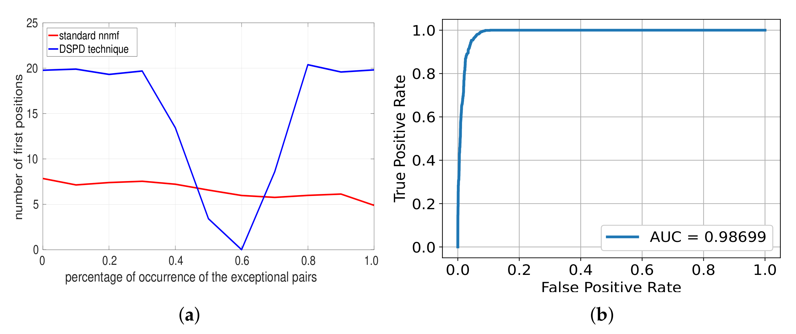
4.1. Synthetic Data

In order to illustrate the behavior of the method, we built a synthetic dataset as follows.

We generate two random matrices each having n rows and m columns, with m ranging from 25 to 500, n ranging from 25 to 500 and $k=n/3$. In particular, one set of experiments is conducted by keeping n fixed to 1000 and by varying m and an other set of experiments is conducted by keeping m fixed to 1000 and by varying n.

Figure 2 reports a comparison with a standard non-negative matrix factorization method and with kernel pca [21], which is an orthogonal linear transformation that transforms the data to a new space such that the greatest variance by some scalar projection of the data comes to lie on the first coordinate, the second greatest variance on the second coordinate, and so on.

Figure 2c,d describes the value of the sum of the former two terms of Equation (1). These terms represent how good the factorization approximates the input matrices, and this is the unique goal of standard nnmf methods. The figure shows that, despite the fact that the goal of our technique is relevantly changed, it is able to provide a good approximation. Indeed, we study the behavior when the number of features changes and the number of words is kept fixed at 1000 and, also, the behavior when the number of features is kept fixed at 10,000 and the number of words change. In both cases, the difference in approximating the original data is very low, witnessing that the proposed modification does not relevantly change the approximation quality.

Figure 2a,b describe the cost of the approximation in terms of discriminating power. Here, we note that the proposed technique is able to detect prototype words much more discriminative than standard methods. This behavior can be observed both when the number of features and when the number of words varies. As for kernel PCA, the coordinates are used as prototypes even if, being designed for other purposes, they are not very effective.

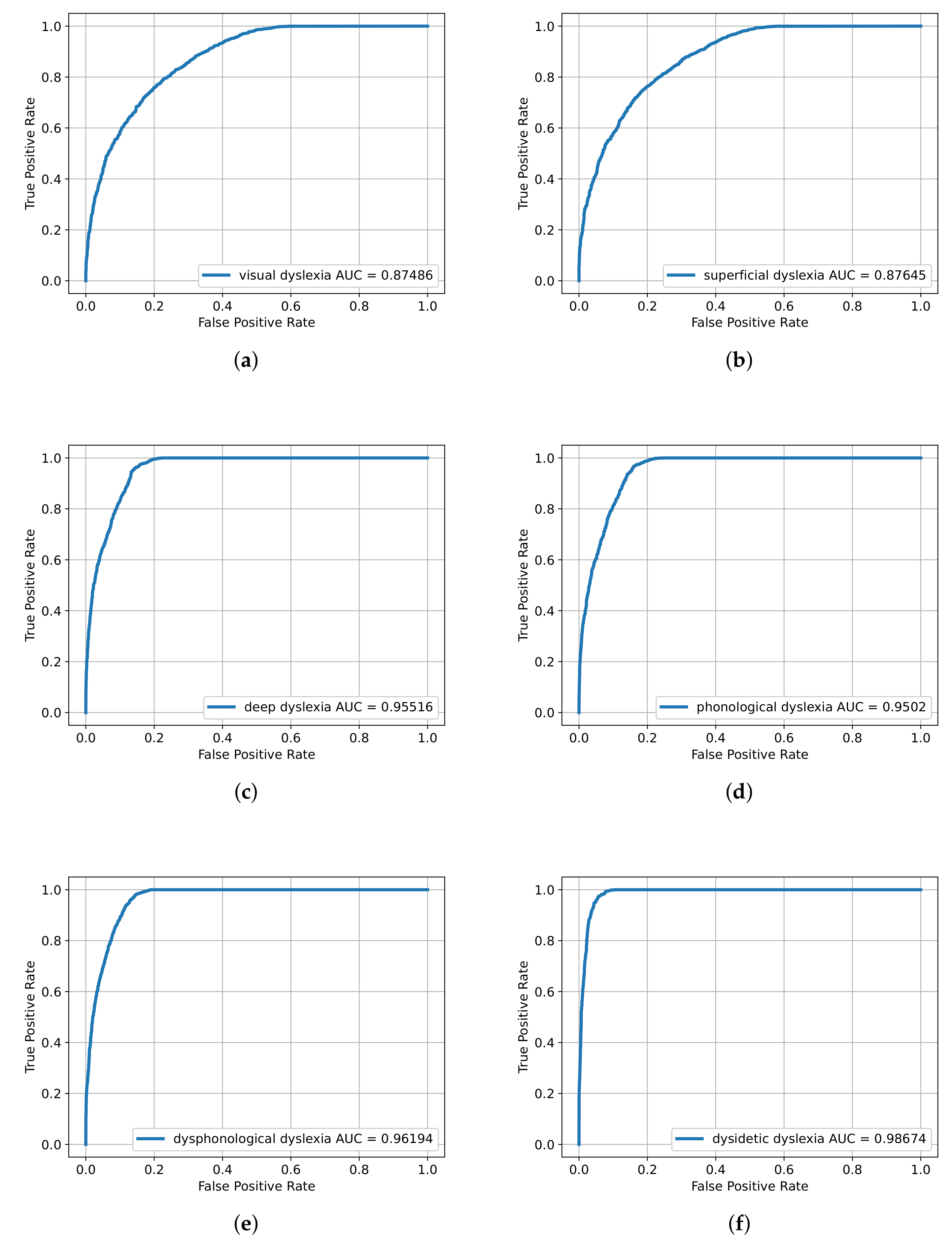
4.2. Real Data

As for the real case of study, we employ data collected and suitably anonymized by an Italian speech therapist center (http://www.logopediatherapeia.it). The tachistoscope used is that described in http://www.iflogos.it/tachistoscopio-flo, since this tool has been developed by the same authors of the present article; in any case, each tachistoscope providing the same information as output can be employed as input module of the presented technique, in particular.

For each patient, the data were collected in three consecutive sessions, and each session provided 75 words. Thus, we have datasets consisting of 225 words.

We started by the groups of two letters individuated by our technique as discriminative and we gained the confirmation by domain experts of disorders related with these pairs.

To prove the ability of the method in individuating interesting pairs, we perform the following experiments. We, first, isolate the words containing the top exceptional pairs. Then, we build a dataset S with the other words and shuffle it. Next, we build the two datasets $W_e$ and $W_r$ with the words coming from S. Iteratively, we inject words containing exceptional pairs in the two datasets with different percentages and measure the rank position of the exceptional pairs, namely we order the entry of the prototypes ${\mathcal{P}}_e^s$ and ${\mathcal{P}}_r^s$ and measure the number of times in which the exceptional pair is in the first position.

Figure 3a reports the results of this experiment. Figure shows that the technique is able to mine a pair of letters just if they have a discriminating power. Indeed, as the occurrence of the pair reaches the $50\%$, namely $W_e$ and $W_r$ are similar with respect to the pair, and the technique does not mine the pair anymore. Vice versa, as for the standard nnmf method, it is not influenced by cross occurrences and then, since the pair is relevant at least in one dataset, it is detected almost always in the same way.

A second part of experiments on real data has concerned the study of the behavior of the proposed technique on recognizing known pathologies. In particular, the algorithm has been fed with datasets referred to individuals with a single known pathology previously diagnosed by experts. In this scenario, the accuracy of the method is measured and results are reported in Figure 3b.

There are different pathologies generating different typologies of errors during tachistoscope sessions, among them

• visual dyslexia;
• superficial dyslexia where lexical pathways are compromised, but reading, although difficult, is possible;
• phonological dyslexia where a phonological path is compromised since a correct association between grapheme and phoneme is missing;
• deep dyslexia where the semantic path is compromised, and semantic paraphasias are performed.
• dysidetic dyslexia where the representation of the word in its variations is difficult, and the new words are not understandable;
• dysphonological dyslexia concerning a deficit at the level of grapheme phoneme mappings.

Figure 4 reports accuracy achieved on recognizing such pathologies. As expected, visual dyslexia and superficial dyslexia are a bit confused since they share some characteristics; conversely, dysidetic dyslexia is the easier to be recognized due to the features related to non-existing words.

However, it is worth noting that, in all cases, the proposed approach achieves significantly good accuracy.

5. Conclusions

The paper presents a technique to mine knowledge from the output of tachistoscopes. These devices provide two sets of words: those correctly answered and those erroneously answered. The addressed problem is to fine intrinsic peculiarities of words able to discriminate between sets of words. Moreover, such peculiarities are used to detect the presence of known pathologies. The proposed technique is based on a novel variant of the non-negative matrix factorization method. Experiments on both synthetic and real data show the effective of the technique and its ability to mine interesting knowledge.

References

- Benschop, R. What Is a Tachistoscope? Historical Explorations of an Instrument. Sci. Context 1998, 11, 23–50. [Google Scholar] [CrossRef] [PubMed]
- Lorusso, M.L.; Facoetti, A.; Toraldo, A.; Molteni, M. Tachistoscopic treatment of dyslexia changes the distribution of visual–spatial attention. Brain Cogn. 2005, 57, 135–142. [Google Scholar] [CrossRef]
- Lorusso, M.L.; Facoetti, A.; Bakker, D.J. Neuropsychological Treatment of Dyslexia: Does Type of Treatment Matter? J. Learn. Disabil. 2011, 44, 136–149. [Google Scholar] [CrossRef] [Green Version]
- Mafioletti, S.; Pregliasco, R.; Ruggeri, L. Il bambino e le abilità di Lettura. Il Ruolo Della Visione; Franco Angeli: Milan, Italy, 2005. [Google Scholar]
- Benso, F.; Berriolo, S.; Marinelli, M.; Guida, P.; Conti, G.; Francescangeli, E. Stimolazione Integrata dei Sistemi Specifi ci per la Lettura e Delle Risorse Attentive Dedicate e del Sistema Attentivo Supervisore; Edizioni Erickson: Trento, Italy, 2008; Volume 5, pp. 167–181. [Google Scholar]
- Nippold, M.A.; Schwartz, I.E. Reading disorders in stuttering children. J. Fluen. Disord. 1990, 15, 175–189. [Google Scholar] [CrossRef]
- Gori, S.; Facoetti, A. Is the language transparency really that relevant for the outcome of the action video games training? Curr. Biol. 2013, 23, 00258-3. [Google Scholar]
- Benso, F. Teoria e Trattamenti nei Disturbi di Apprendimento; Tirrenia (Pisa) Del Cerro: Pisa, Italy, 2004. [Google Scholar]
- Benso, F. Sistema Attentivo-Esecutivo e Lettura. Un Approccio Neuropsicologico alla Dislessia; Il leone verde: Torino, Italy, 2010. [Google Scholar]
- Sharma, M.; Purdy, S.; Kelly, A. Comorbidity of Auditory Processing, Language, and Reading Disorders. J. Speech Lang. Hear. Res. JSLHR 2009, 52, 706–722. [Google Scholar] [CrossRef] [Green Version]
- Yadav, N.; Poellabauer, C.; Daudet, L.; Collins, T.; McQuillan, S.; Flynn, P. Portable Neurological Disease Assessment Using Temporal Analysis of Speech. In Proceedings of the 6th ACM Conference on Bioinformatics, Computational Biology and Health Informatics, Atlanta, GA, USA, 9–12 September 2015; Association for Computing Machinery: New York, NY, USA, 2015. BCB ’15. pp. 77–85. [Google Scholar]
- Cagatay, M.; Ege, P.; Tokdemir, G.; Cagiltay, N.E. A serious game for speech disorder children therapy. In Proceedings of the 2012 7th International Symposium on Health Informatics and Bioinformatics, Nevsehir, Turkey, 19–22 April 2012; pp. 18–23. [Google Scholar]
- Pervaiz, M.; Patel, R. SpeechOmeter: Heads-up monitoring to improve speech clarity. In Proceedings of the 16th International ACM SIGACCESS Conference on Computers and Accessibility, Rochester, NY, USA, 20–22 October 2014; pp. 319–320. [Google Scholar]
- Wang, Y.X.; Zhang, Y.J. Nonnegative Matrix Factorization: A Comprehensive Review. IEEE Trans. Knowl. Data Eng. 2013, 25, 1336–1353. [Google Scholar] [CrossRef]
- Kim, J.; He, Y.; Park, H. Algorithms for nonnegative matrix and tensor factorizations: A unified view based on block coordinate descent framework. J. Glob. Optim. 2014, 58, 285–319. [Google Scholar] [CrossRef] [Green Version]
- Kim, H.; Choo, J.; Kim, J.; Reddy, C.K.; Park, H. Simultaneous Discovery of Common and Discriminative Topics via Joint Nonnegative Matrix Factorization. In Proceedings of the ACM SIGKDD International Conference on Knowledge Discovery and Data Mining, Sydney, Australia, 10–13 August 2015; pp. 567–576. [Google Scholar]
- Berry, M.W.; Castellanos, M. Survey of Text Mining II: Clustering, Classification, and Retrieval, 1st ed.; Springer: Berlin/Heidelberg, Germany, 2007. [Google Scholar]
- Long, Y.H.; Dai, L.R.; Wang, E.Y.; Ma, B.; Guo, W. Non-negative matrix factorization based discriminative features for speaker verification. In Proceedings of the International Symposium on Chinese Spoken Language Processing, Tainan, Taiwan, 10 January 2010; pp. 291–295. [Google Scholar]
- Zhang, Z.Y. Nonnegative Matrix Factorization: Models, Algorithms and Applications. In Data Mining: Foundations and Intelligent Paradigms: Volume 2: Statistical, Bayesian, Time Series and Other Theoretical Aspects; Holmes, D.E., Jain, L.C., Eds.; Springer: Berlin/Heidelberg, Germany, 2012; pp. 99–134. [Google Scholar]
- Hulme, C.; Snowling, M.J. Reading disorders and dyslexia, Current Opinion in Pediatrics. Neurology 2016, 28, 731–735. [Google Scholar]
- Schölkopf, B.; Smola, A.J.; Müller, K.R. Nonlinear Component Analysis as a Kernel Eigenvalue Problem. Neural Comput. 1998, 10, 1299–1319. [Google Scholar] [CrossRef] [Green Version]
Publisher’s Note: MDPI stays neutral with regard to jurisdictional claims in published maps and institutional affiliations. |
© 2022 by the authors. Licensee MDPI, Basel, Switzerland. This article is an open access article distributed under the terms and conditions of the Creative Commons Attribution (CC BY) license (https://creativecommons.org/licenses/by/4.0/).
Share and Cite
Fassetti, F.; Fassetti, I. Discriminating Pattern Mining for Diagnosing Reading Disorders. Appl. Sci. 2022, 12, 7540. https://doi.org/10.3390/app12157540
Fassetti F, Fassetti I. Discriminating Pattern Mining for Diagnosing Reading Disorders. Applied Sciences. 2022; 12(15):7540. https://doi.org/10.3390/app12157540
Chicago/Turabian StyleFassetti, Fabio, and Ilaria Fassetti. 2022. "Discriminating Pattern Mining for Diagnosing Reading Disorders" Applied Sciences 12, no. 15: 7540. https://doi.org/10.3390/app12157540