
Research on a Wi-Fi RSSI Calibration Algorithm Based on WOA-BPNN for Indoor Positioning


1
College of Software, Jiangxi Normal University, Nanchang 330022, China
2
College of Information Engineering, Jiangxi University of Technology, Nanchang 330098, China
3
State Key Laboratory of Information Engineering in Surveying, Mapping and Remote Sensing, Wuhan University, Wuhan 430079, China
*
Author to whom correspondence should be addressed.
Appl. Sci. 2022, 12(14), 7151; https://doi.org/10.3390/app12147151
Submission received: 15 June 2022
/
Revised: 11 July 2022
/
Accepted: 14 July 2022
/
Published: 15 July 2022
(This article belongs to the Topic Multi-Sensor Integrated Navigation Systems)
Abstract
:Owing to the heterogeneity of software and hardware in different types of mobile terminals, the received signal strength indication (RSSI) from the same Wi-Fi access point (AP) varies in indoor environments, which can affect the positioning accuracy of fingerprint methods. To solve this problem and consider the nonlinear characteristics of Wi-Fi signal strength propagation and attenuation, we propose a whale optimisation algorithm-back-propagation neural network (WOA-BPNN) model for indoor Wi-Fi RSSI calibration. Firstly, as the selection of the initial parameters of the BPNN model has a considerable impact on the positioning accuracy of the calibration algorithm, we use the WOA to avoid blindly selecting the parameters of the BPNN model. Then, we propose an improved nonlinear convergence factor to balance the searchability of the WOA, which can also help to optimise the calibration algorithm. Moreover, we change the structure of the BPNN model to compare its influence on the calibration effect of the WOA-BPNN calibration algorithm. Secondly, in view of the low positioning accuracy of indoor fingerprint positioning algorithms, we propose a region-adaptive weighted K-nearest neighbour positioning algorithm based on hierarchical clustering. Finally, we effectively combine the two proposed algorithms and compare the results with those of other calibration algorithms such as the linear regression (LR), support vector regression (SVR), BPNN, and genetic algorithm-BPNN (GA-BPNN) calibration algorithms. The test results show that among different mobile terminals, the proposed WOA-BPNN calibration algorithm can increase positioning accuracy (one sigma error) by 41%, 42%, 44% and 36%, on average. The indoor field tests suggest that the proposed methods can effectively reduce the indoor positioning error caused by the heterogeneous differences of software and hardware in different mobile terminals.
1. Introduction
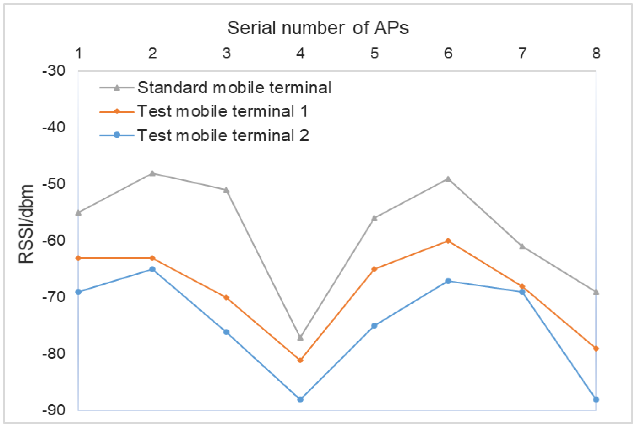
With the rapid development of society, people are spending most of their time in indoor environments such as shopping malls and office buildings. Owing to the weak global navigation satellite system (GNSS) signals received indoors, accurate indoor positioning via GNSS is not possible [1]. Currently, indoor positioning has become a research hotspot. In the field of indoor positioning, fingerprint positioning was verified to be a feasible method for indoor positioning [2]. Considering the deployment cost and indoor positioning accuracy, the indoor positioning method based on Wi-Fi signal is currently the most widely used. However, owing to the heterogeneity of software and hardware between different mobile terminals, the signal strength indication (RSSI) values received by different mobile terminals from the same Wi-Fi access point (AP) at the same location differ considerably, as shown in Figure 1, which will have a serious impact on indoor positioning accuracy. To solve the above problems and improve indoor positioning accuracy, calibrating the Wi-Fi RSSI values received by different mobile terminals at the same position is necessary to make the RSSI values consistent.
For indoor positioning and calibration, He et al. [3] proposed recording the signal strength collected by different mobile terminals and using linear regression (LR) model to calibrate the difference between different mobile terminals, which could help improve positioning accuracy. However, owing to the nonlinear logarithmic variation in RF signal strength with distance and the simple linear calibration method, the positioning accuracy was poor. Therefore, an increasing number of scholars are examining nonlinear indoor positioning and calibration algorithms. Li et al. [4] proposed a new algorithm that used support vector regression (SVR) to construct the nonlinear mapping relation between the RSSI and distance between tags and readers. Song et al. [5] proposed the possibility of the nonlinear calibration of Wi-Fi signals by establishing a back-propagation neural network (BPNN) model. Through repeated training, this method can obtain a relatively stable BPNN calibration model, but the improper selection of the initial parameters of a BPNN model will lead to poor calibration results. To solve this problem, Yu et al. [6] proposed to further optimise the initial weights and thresholds of a BPNN model by using the selection and mutation process of a genetic algorithm (GA) to overcome the problem of the BPNN model falling easily into local optimisation. Although the above algorithms can reduce the error caused by the heterogeneity of software and hardware in different mobile terminals, several parameters must be set for a GA-BPNN model, which at present are selected empirically.
In the online phase, if the positioning area is large and the spacing of the fingerprint reference points is dense, then matching the RSSI data collected from a real-time location to each fingerprint data in the fingerprint database will lead to a large number of calculations and will be unable to obtain the positioning results immediately. To reduce the fingerprint point matching calculation and determine the current position in a certain area quickly, some scholars used a clustering algorithm in the indoor positioning process to roughly realise the location. Ferreira et al. [7] applied a K-nearest neighbour (KNN) classification method to improve the performance of indoor localization. Xue et al. [8] utilised a K-means clustering algorithm to analyse the geometric proximity between the reference point and test point in the online phase. Zhao et al. [9] combined naive Bayes classifier (NBC) and weighted KNN (WKNN) to achieve indoor positioning, which obtained a better result than the traditional indoor positioning systems (IPSs). However, these methods must set the appropriate value of K in advance. If the value of K is not set properly, it will have a certain negative impact on the subsequent positioning results. Li et al. [10] proposed the improved fuzzy c-means algorithm for regional division in the offline training phase, which introduces the K-means clustering algorithm and between–within proportion (BWP) index to select the optimal initial clustering centre and number of clusters. He et al. [11] proposed a regional division method based on a Voronoi graph that is constructed with the initial reference points as the generating points, and the virtual reference points are partitioned into the nearest Voronoi region.
To effectively solve the above problems, the main work of this paper is as follows:
- (1)
- Firstly, we propose a Wi-Fi RSSI calibration algorithm based on a whale optimisation algorithm (WOA)-BPNN and use the WOA to find the optimal initial weights and thresholds of the BPNN model. The proposed algorithm has a simple process and few parameters to adjust. Secondly, to speed up the establishment and optimisation of the calibration algorithm and upgrade the updating and iterating speed, we propose a nonlinear convergence factor a to simulate the shrinking behaviour of the surrounding prey of the whales and obtain an improved WOA-BPNN calibration algorithm. The convergence factor a changes dynamically only with the current iterations t and effectively prevents the algorithm from falling into the local optimum. We use the calibration algorithm to calibrate the Wi-Fi RSSI data received by the different mobile terminals at the same position to make the Wi-Fi RSSI consistent. Finally, by changing the hidden layer structure of the BPNN model, we compare the performance of different BPNN models on the calibration results.
- (2)
- Focusing on the problem of the low positioning accuracy of location fingerprint indoor positioning algorithms based on the Wi-Fi RSSI, we propose a region-adaptive weighted KNN (WKNN) positioning algorithm based on hierarchical clustering. Firstly, we employ the BWP index to evaluate the clustering results and find the optimal number of clustering regions, which can help narrow the online matching positioning range and improve the positioning speed. Secondly, this algorithm adaptively determines the K fingerprint data in the fingerprint database of its attribution area, which is similar to the RSSI values received by the mobile terminals at a real-time position, then uses the WKNN algorithm to calculate the final position results comprehensively.
To verify the effectiveness of the two proposed algorithms we further combine the WOA-BPNN calibration algorithm (in which the hidden layers of BPNN are double layers and the number of neurons in each layer is six) with the region-adaptive WKNN position algorithm based on hierarchical clustering, and compare the average positioning error obtained after calibration with those of three other positioning algorithms (i.e., NN, KNN and WKNN) and four other calibration algorithms (i.e., LR, SVR, BPNN and GA-BPNN). The experiments show that the combination of the WOA-BPNN calibration algorithm and region-adaptive positioning WKNN algorithm based on hierarchical clustering can effectively reduce the indoor positioning error caused by the heterogeneity of software and hardware in different mobile terminals, thereby improving the availability and universality of the calibration algorithm.
2. Methods and Algorithms
2.1. Methods
2.1.1. BPNN
A BPNN is a neural network trained according to the error back-propagation algorithm, consisting of an input layer, several hidden layers and an output layer [12]. Each layer can have several neurons, and the connection state of the neurons between the layers is reflected by the weights. A BPNN is a multilayer feedforward neural network with a strong learning ability that can be used to process the complex mapping relationships of nonlinear functions and is often used in classification or prediction problems. Selami et al. [13] employed a BPNN model to reduce the effect of the nonlinearities presented in laser triangulation displacement sensors. Hu et al. [14] developed a BPNN model to correct heading angle velocity output and vehicle speed and to add the synthesized relative displacement to the previous absolute position to realize a new vehicle position. Moreover, based on BPNN model, Xing et al. [15] proposed a 60 GHz impulse radio positioning algorithm, which has obtained a good positioning result.
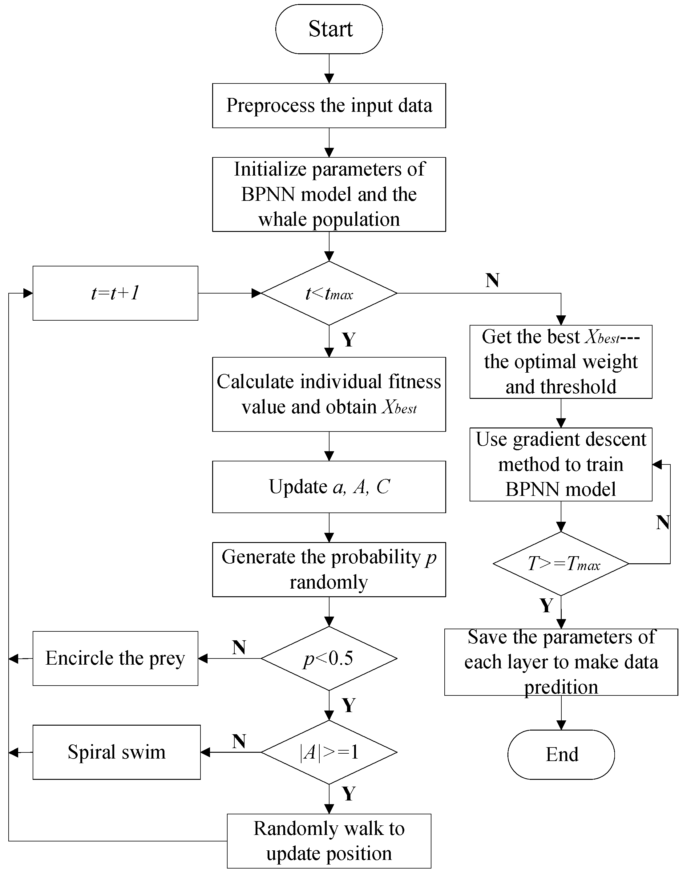
Differing from the above algorithms, in this study we apply a BPNN model to indoor Wi-Fi RSSI calibration that corrects the Wi-Fi RSSI values received by different mobile terminals based on the standard mobile terminal. Firstly, we utilise a WOA to help the BPNN model find the optimal initial weights and thresholds. Secondly, to speed up the establishment and optimisation of the calibration algorithm and to increase the updating and iterating speed, we propose a nonlinear convergence factor, a. The model principle is shown in Figure 2, and the algorithm steps are explained in Section 2.2.1.
2.1.2. WOA
The WOA is a novel swarm intelligence optimisation algorithm based on the behaviour of whales hunting prey proposed by Mirjalili and Lewis in 2016 [16]. When hunting, whale populations cooperate with one another to drive and surround their prey. In the WOA, the position of each whale represents a feasible solution. During the hunting process of a whale population, each whale will randomly choose from two behaviours to update its position. The first behaviour is to surround the prey, in which the whales will randomly swim towards the best position to hunt the prey or randomly select a whale as their target and swim to it. The second behaviour is to create a bubble net, in which the whales swim in a circular motion and release bubbles to drive away their prey. In each iteration, the whales will randomly choose from the two behaviours to hunt.
2.1.3. Agglomerative Hierarchical Clustering Method
The agglomerative hierarchical clustering method, a ’bottom-up’ clustering method [17] that first treats each fingerprint point in the offline fingerprint database as a separate class, then calculates the distance between every two points and selects the two closest classes to merge into a new class, and repeats the process continuously. The merging stops when the termination condition is reached. The advantage of this clustering method is that it demonstrates satisfactory flexibility, that is, setting the number of clusters in advance is unnecessary. After setting the appropriate termination conditions, we will likely obtain the required clustering results. The calculation of the distance between different classes generally adopts several methods, such as the minimum distance dmin, maximum distance dmax and average distance davg. Owing to the instability of Wi-Fi RSSI in indoor environments, the RSSI collected from two points far away may have certain similarities, so we adopt the agglomerated hierarchical clustering method of average distance (average-linkage), and divide the fingerprint database into regions according to the Euclidean distance between every two fingerprint points, thereby avoiding matching to fingerprint points that are far away in the online positioning phase.
2.2. Algorithms
2.2.1. Calibration Algorithm Based on WOA-BPNN
As a WOA uses few parameters to achieve quick convergence and does not easily encounter the local optimum problem, we employ it to optimise the BPNN model and model the problem of the parameter selection of the BPNN model as parameter optimisation. We establish an objective function to optimise the combination of parameters and use the WOA to search for the optimal parameters, that is, the optimal initial weights and thresholds of the BPNN model.
- (1)
- A New Convergence Factor
The WOA includes two processes: global searching and local searching. If the algorithm is intended for global searching, then it can keep the diversity of group and avoid falling into local optimum; if it is intended for local searching, then it can search precisely and speed up the search process. The searchability of the WOA depends on the value of |A|, and the value of |A| varies with the change of the convergence factor a, see Equation (3) for the relationship between A and a. A larger convergence factor will improve the ability of global searching ability and reduce the possibility of premature maturity of the algorithm. By contrast, a small convergence factor will improve the local searching ability and efficiency of the algorithm.
The convergence factor of a traditional WOA changes linearly, but in the actual searching process, the WOA changes non-linearly and causes slow convergence. Therefore, to speed up the establishment and optimisation of the calibration algorithm and increase the updating and iterating speed, we propose a nonlinear convergence formula [18] that simulates the shrinking behaviour of the surrounding prey of the whales, as shown in Equation (1), where the convergence factor a changes dynamically only with the current number of iterations of whale population t, which can effectively prevent the algorithm from falling into the local optimum.
where t is the current number of iterations of the whale population and tmax is the maximum number of iterations of the whale population.
- (2)
- WOA-BPNN Calibration Algorithm Steps
As one of the most successful neural network learning algorithms, a BPNN demonstrates satisfactory robustness and generalisation ability. However, the improper selection of initial weights and thresholds will cause a BPNN model to fall into a local optimum, thereby resulting in poor calibration results. Wang et al. [19] utilised the global search capability of the mind evolutionary algorithm to determine the initial weights and thresholds of a BPNN model. Zhang et al. [20] employed the ant colony algorithm to optimise the initial weights and thresholds of a BPNN model then established a calibration model. Owing to its characteristics of few parameters, ability to jump out of the local optimum and satisfactory convergence ability, we employ the WOA as well as an improved convergence factor a [21] to optimise the parameters of the BPNN model. The algorithm steps are presented below (refer to Figure 2).
- Step 1: Randomly select several acquisition points in the room and use a standard mobile terminal and test mobile terminal to collect the RSSI values of all APs at all acquisition points. To reduce the noise impact of personnel disturbance and same frequency interference during the RSSI propagation, process the received multiple RSSI values of the same AP via mean filtering. Take the average RSSI values of each AP collected from all acquisition points by the standard mobile terminal as the initial standard sampling data and take the average RSSI values of all the corresponding APs of the test mobile terminal at the corresponding acquisition points as the test sampling data. In addition, take the test sampling data as the real input value of the WOA-BPNN calibration model and take the initial standard sampling data as the real output value of the WOA-BPNN calibration model.
- Step 2: Initialise the weight and threshold of each layer randomly to build the BPNN, which also means initialising the whale group position . Next, set the size of the whale population N, the current number of iterations of the whale population , the maximum number of iterations of the whale population , the current number of iterations of the BPNN model , and the maximum number of iterations of the BPNN model .
- Step 3: When the current number of iterations of the whale population t is less than the maximum iteration number of the whale population, according to the fitness function formula, as Equation (2), calculate the fitness value of each whale, obtain the position of the optimal fitness value, and then find the best fitness and the corresponding optimal whale position .where is the real value of the ith RSSI, is the predicted value of the ith RSSI and is the number of samples.
- Step 4: To speed up the establishment and optimisation of the calibration algorithm and upgrade the updating and iterating speed, use the proposed nonlinear convergence factor a to simulate the shrinking behaviour of the surrounding prey of the whales. The convergence factor a changes dynamically only with the current iteration times t and effectively prevents the algorithm from falling into the local optimum. The formula of the nonlinear convergence factor a is shown as Equation (1). Update the whale position parameters A and C. The formulas are shown in Equations (3) and (4).where r is a random value of [0, 1].
- Step 5: Randomly generate probability p and judge whether it is less than 0.5. If , then update the position by shrinking and surrounding, as shown in Equation (5).where t is current number of iterations of the whale population, is the optimal whale position, is the current whale position and and are the whale position parameters obtained in Step 4, else if , then select the swimming mode according to the value of |A|: when , the whales will choose to update their position by swimming in a circular motion, as shown in Equation (6).where indicates the distance between the whale and the optimal position, is a constant that defines the logarithmic spiral shape and is a random value in [–1, 1]; when , the whales choose to swim randomly according to Equation (7):where is the randomly selected position of a whale.
- Step 6: The current number of iterations of the whale population t increases automatically, and the optimal position is updated according to Step 2. When the maximum number of iterations of the whale population is reached, it outputs , which represents the optimal weight and threshold as the optimal initial parameters of the BPNN model.
- Step 7: The BPNN performs forward propagation, processing data through the connection weight between the neuron i and the neuron j and threshold of the neuron j. Obtain the predicted output value using the nonlinear sigmoid activation function, as shown in Equations (8) and (9), as follows:where is the connection weight between the neuron and the neuron , , and are the threshold, input value and output value of the neuron , respectively, and is the input value of the neuron and is the number of samples.
- Step 8: With the forward propagation process, we obtain the predicted value of the output layer neuron. According to the error between the predicted output value and the real output value, obtain the loss function of the current iteration number , as shown in Equation (10); the error is propagated back to the upper layer of neurons to obtain the error in this layer, and then passes layer by layer until the top hidden layer is reached. Update and adjust the connection weights and thresholds based on the gradient descent method, as shown in Equations (11) and (12), as follows:where is the real output value of the output layer neuron j, is the predicted output value of the output layer neuron j, is the number of samples, is the updated weight between the neuron i and the neuron j, is the updated threshold of the neuron j, and is the learning rate, if is too large, the convergence will be fast but easy to fall into the local optimum, if the value is too small, the convergence will be slow but close to the global optimum.
- Step 9: After repeated learning and training, when the current number of iterations of the BPNN model T reaches the maximum number of iterations of the BPNN model Tmax, select the BPNN model with the smallest loss function as the final calibration model, and save the parameters of the current WOA-BPNN calibration model and corresponding mobile terminal model.
- Step 10: Repeat Step 1 to Step 8 for multiple mobile terminals, then establish the calibration model database.
2.2.2. Region-Adaptive WKNN Algorithm Based on Hierarchical Clustering
The WKNN algorithm is a further improvement based on the K-nearest neighbour (KNN) algorithm [22]. Different weighting factors are set according to the Euclidean distance of different fingerprint reference points relative to the current position. Compared with other fingerprint-based positioning algorithms, the WKNN algorithm has better positioning accuracy and stability. However, regardless of whether the WKNN or KNN algorithm is used, when performing the actual positioning, determining the value of K, which is the number of neighbouring reference points, is necessary. The value of K has an important influence on the positioning result. Thus, we propose an adaptive WKNN method that can utilise the feature of the Euclidean distance and physical coordinates between the real-time position and RSSI of the fingerprint database to adjust the value of K dynamically during the online positioning process, which can help to improve the positioning stability and obtain the best positioning accuracy.
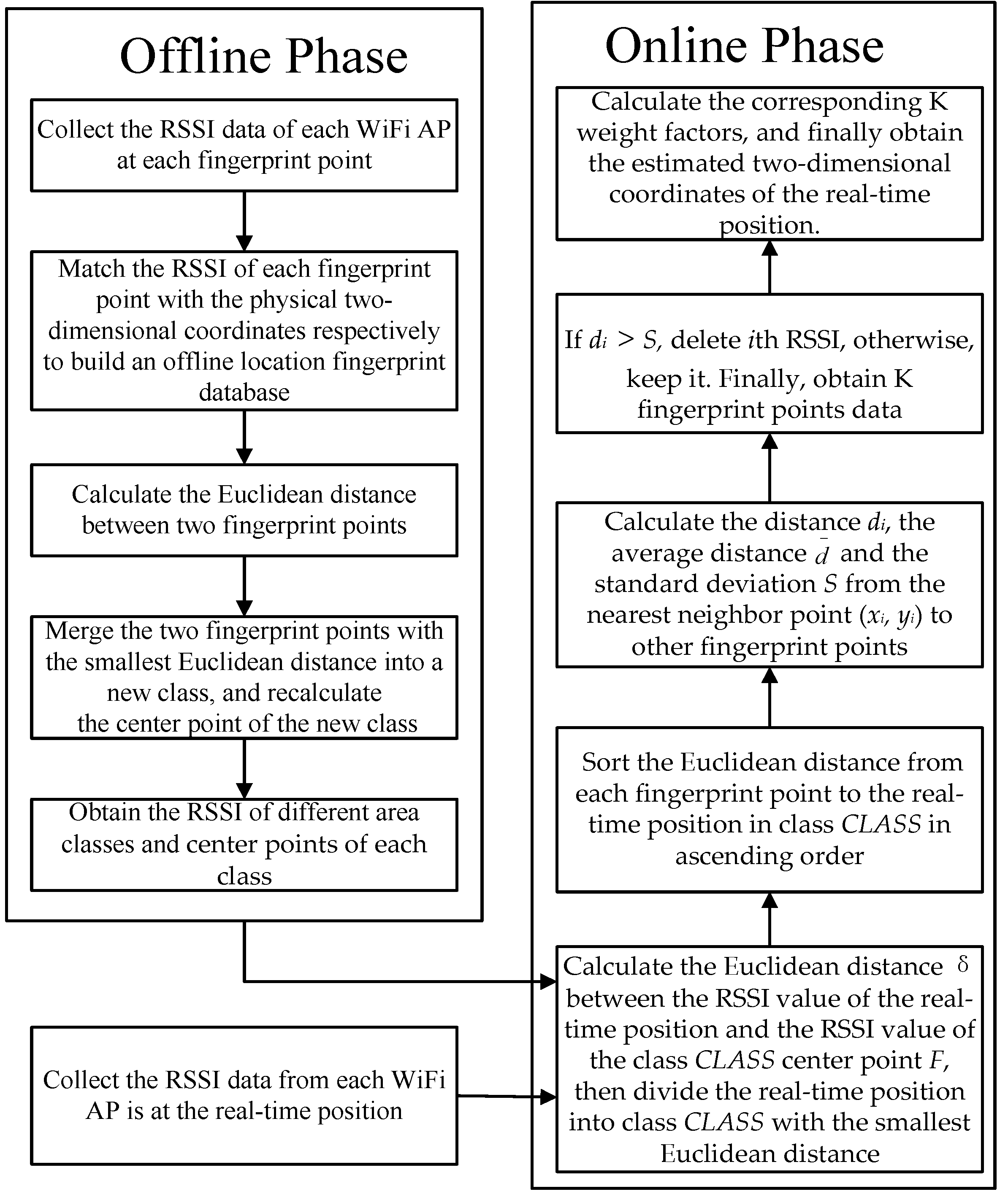
The algorithm steps of the region-adaptive WKNN algorithm based on hierarchical clustering are shown in Figure 3, and its process is described as follows:
- Step 1: In the offline phase, a mobile terminal collects the average RSSI data of each Wi-Fi AP at each fingerprint point, match the RSSI of each fingerprint point with the physical two-dimensional coordinates to build an offline location fingerprint database.
- Step 2: Calculate the Euclidean distance between two fingerprint points, then merge the two fingerprint points with the smallest Euclidean distance into a new class and recalculate the centre point of the new class. Finally, obtain the RSSI of different area classes and centre points of each class.
- Step 3: In the online phase, the mobile terminal collects RSSI values from each Wi-Fi AP at a real-time position to form a set of RSSI data. Calculate the Euclidean distance D between the RSSI value of the real-time position and the RSSI value of the class CLASS centre point F in turn, as shown in Equation (13), then divide the real-time position into the class CLASS with the smallest Euclidean distance.where rssij is RSSI value of the jth Wi-Fi AP collected from the real-time position, RSSIFj is the RSSI value of the jth Wi-Fi AP of the CLASS centre point F of class, and n is the number of Wi-Fi APs.
- Step 4: Sort the Euclidean distance from each fingerprint point to the real-time position in class CLASS in ascending order. Find the corresponding two-dimensional coordinates (x1, y1) of the fingerprint points, calculate the distance , the average distance and the standard deviation from the nearest neighbour point to the other fingerprint points, as shown in Equations (14)–(16).
- Step 5: Filter the fingerprint points in class C further. When , delete the ith RSSI, otherwise, when , keep the ith RSSI. Finally, obtain K fingerprint points data, n is the number of Wi-Fi AP.
- Step 6: According to the Euclidean distance of the remaining K fingerprint points, calculate the corresponding weight factor and obtain the estimated two-dimensional coordinates of the real-time position.
3. Experiments and Results
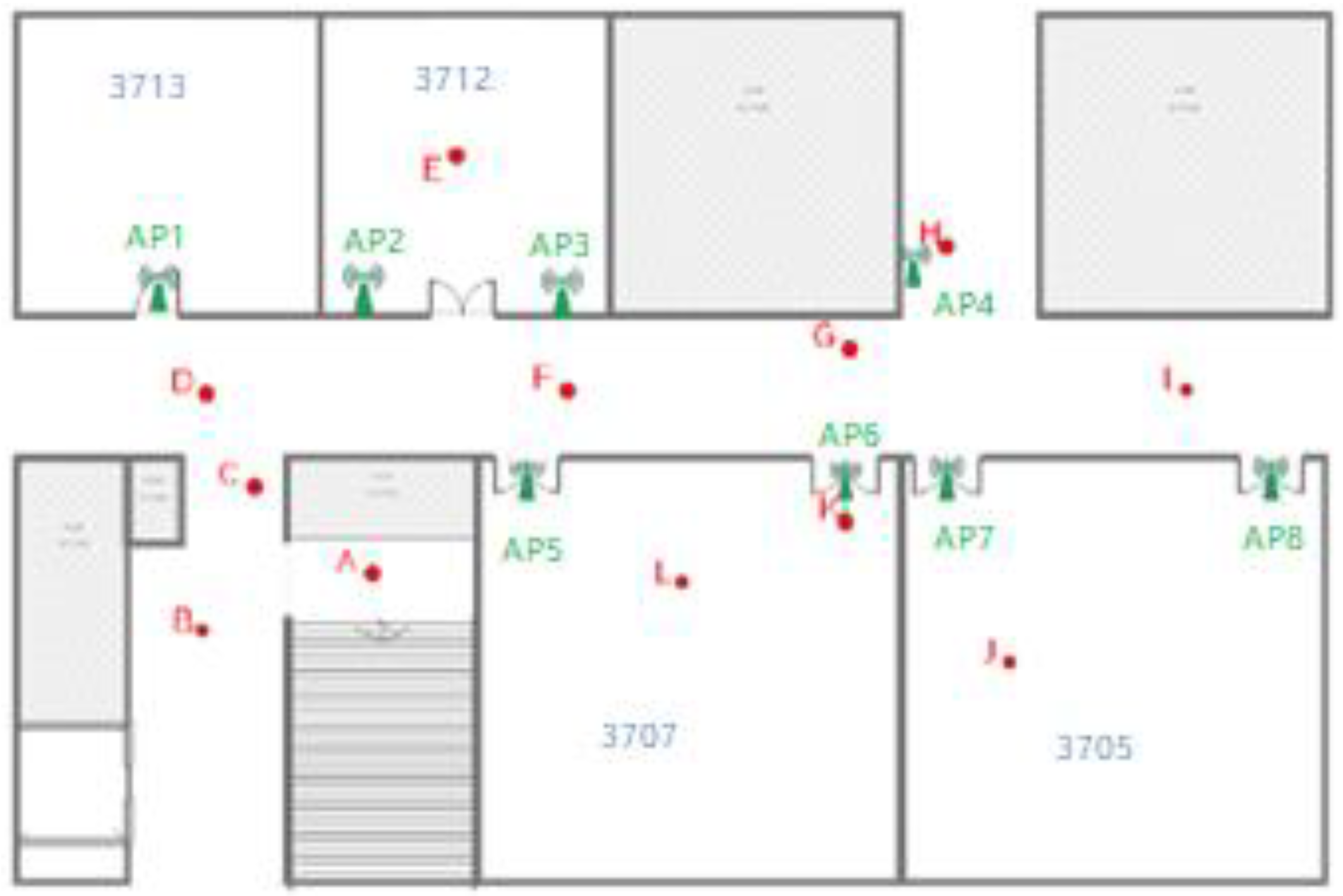
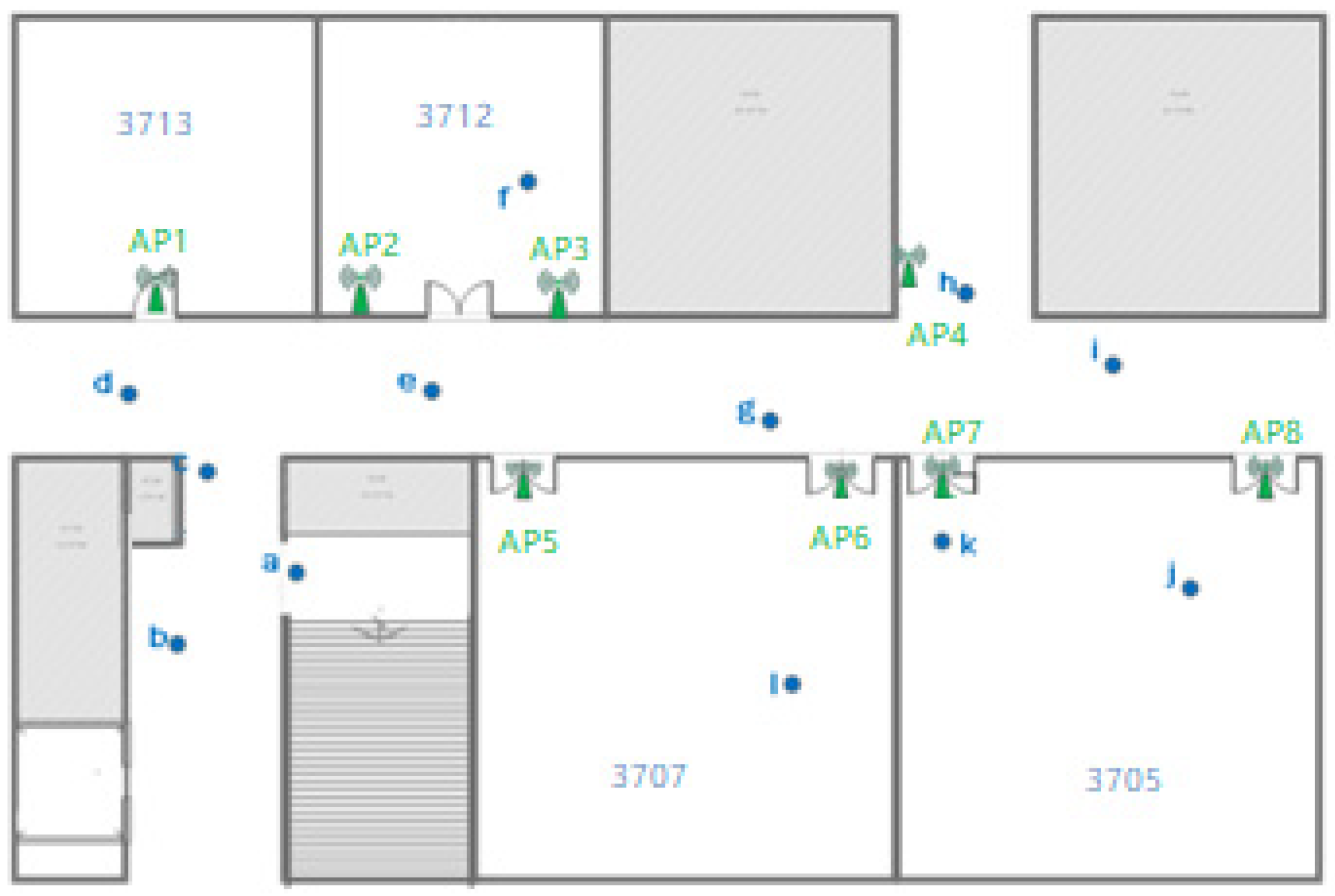
Our experimental environment is the seventh floor of the XianSu Building at the Yaohu campus of Jiangxi Normal University, which includes a corridor (3 m × 21.5 m); four laboratories, specifically, rooms 3705 (7 m × 7 m), 3707 (7 m × 7 m), 3712 (7 m × 7 m) and 3713 (7 m × 7 m); and a corner. We arrange eight TL-WR885N routers on the wall at a height of 2.1 m as the Wi-Fi RSSI signal access points (AP1-AP8). The mobile terminals used in the experiment include a standard mobile terminal (Huawei mate10pro), test mobile terminal 1 (Huawei mate8) and test mobile terminal 2 (Huawei P8), all of which contain Wi-Fi sensors.
3.1. Wi-Fi AP Number Setting
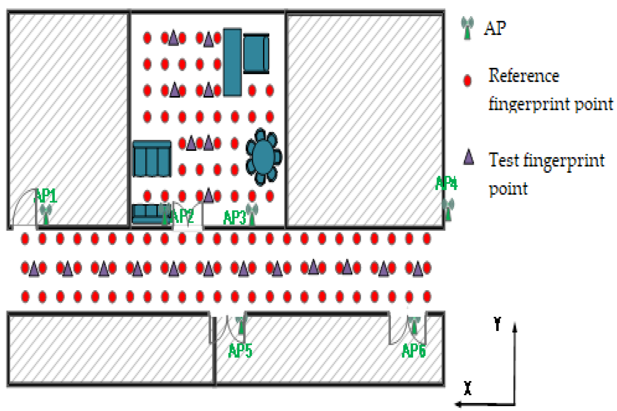
To explore the influence of the number of Wi-Fi APs used to build the model on the calibration effect of the WOA-BPNN calibration algorithm, we select 12 modelling points and 12 test points randomly for the experiments at the experiment area described above. The distribution of the modelling points (red dots), test points (blue dots) and APs (green icons) is shown in Figure 4 and Figure 5.
Under different numbers of Wi-Fi APs (1–8), we use the standard mobile terminal and test mobile terminals to collect the Wi-Fi RSSI modelling data at the modelling points at a frequency of 30 s/time for 6 min. We use the standard mobile terminal and two test mobile terminals to collect the test data at the test points using the same method. We average all the RSSI data received from each AP in the data sample collected at each acquisition point (for each AP, we obtain only one average RSSI value at each point after mean filter processing; we process the subsequent obtained RSSI data in the same way) and take the average RSSI value of each AP as the RSSI value of the acquisition point. In establishing the calibration model, we take the modelling data of the test mobile terminals (test mobile terminal 1 or test mobile terminal 2) as the input value of the calibration model and the modelling data of the standard mobile terminal as the real output value of the calibration model. The model generates the predicted output data after the modelling data of the test mobile terminals pass through the calibration model, then compares and calculates the error between the predicted output data and real output value, which are then propagated back to the calibration model. Finally, we obtain a stable calibration model after continuous adjustment. Therefore, we get the calibration model of the standard mobile terminal–test mobile terminal 1 and standard mobile terminal–test mobile terminal 2. After establishing the calibration model, we use the test data of the two test mobile terminals as the input value of the calibration model to apply the corresponding model for the RSSI calibration. Finally, we calculate the error between the test data of the standard mobile terminal and test data of the test mobile terminals as well as the error between the data of the test mobile terminals after calibration and those of the standard mobile terminal. We analyse the error reduction ratio p value of the RSSI calibration model for different numbers of APs.
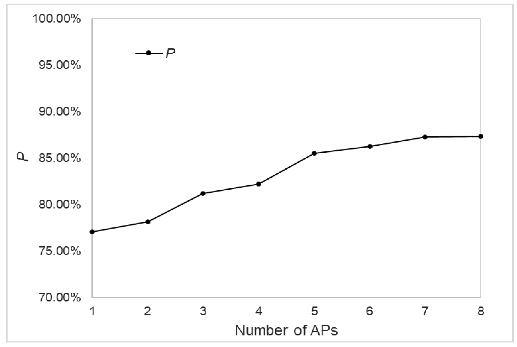
where is the error between RSSI value of the test mobile terminal and that of the standard mobile terminal before calibration; is the error between the RSSI value of the test mobile terminal after calibration and that of the standard mobile terminal; is the number of error reduction after calibration in the test data; Z is the total number of test data sets, which is proportional to the number of APs.
Figure 6 shows that when the number of Wi-Fi APs continues to increase, the error reduction ratio p value also increases. When the number of Wi-Fi APs equals one, the error reduction ratio p of the RSSI calibration is the worst value, which shows that the calibration model established with a single AP is unstable. Meanwhile, when the number of APs increases from one to five, the value of p increases rapidly; when the number of APs reaches six or more, the increase of the error reduction ratio p value is small for each additional number of modelling APs. Therefore, considering the calibration efficiency and actual calculation amount, this experiment shows that selecting five or six modelling APs for modelling and calibration is appropriate.
3.2. Region Division Result
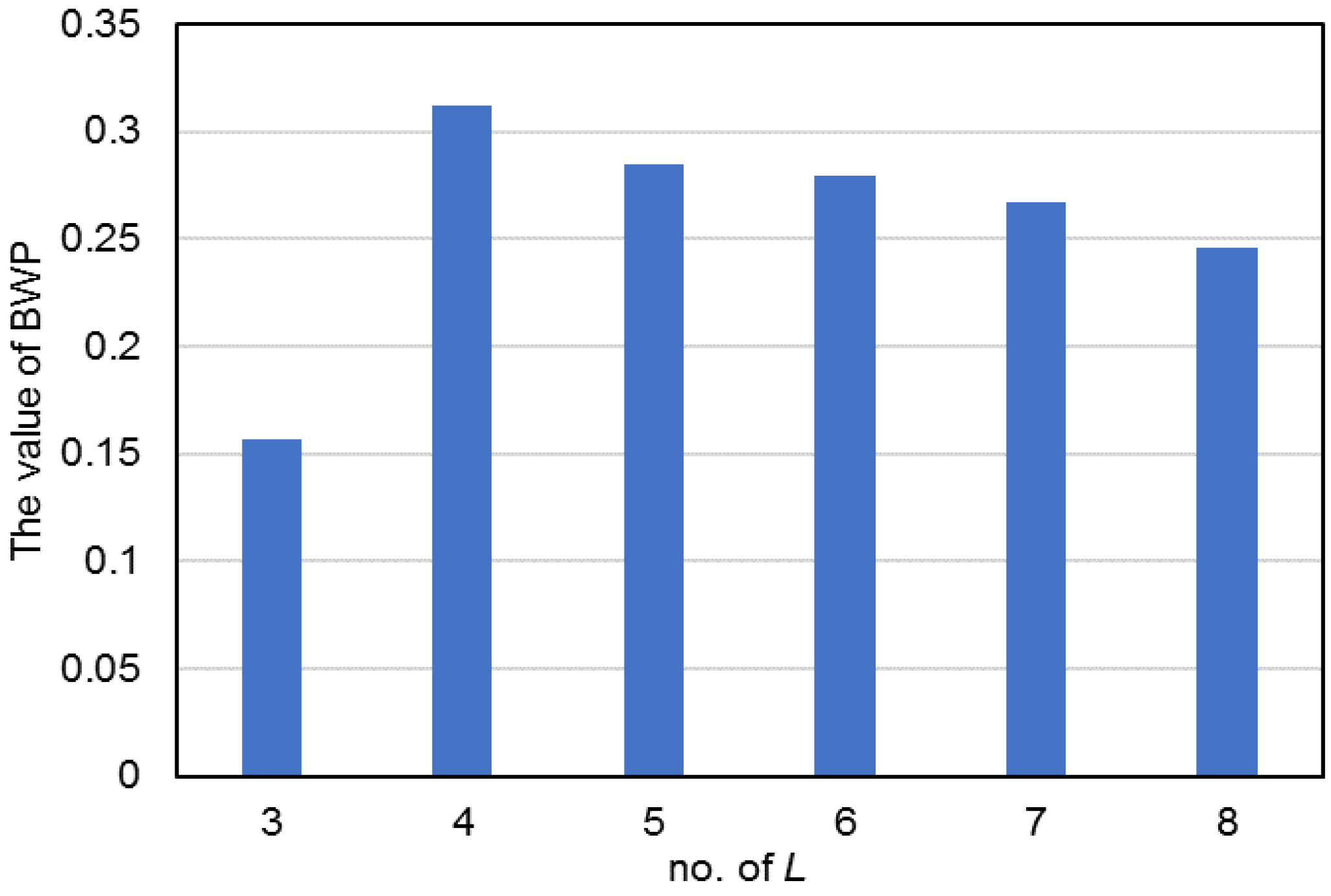
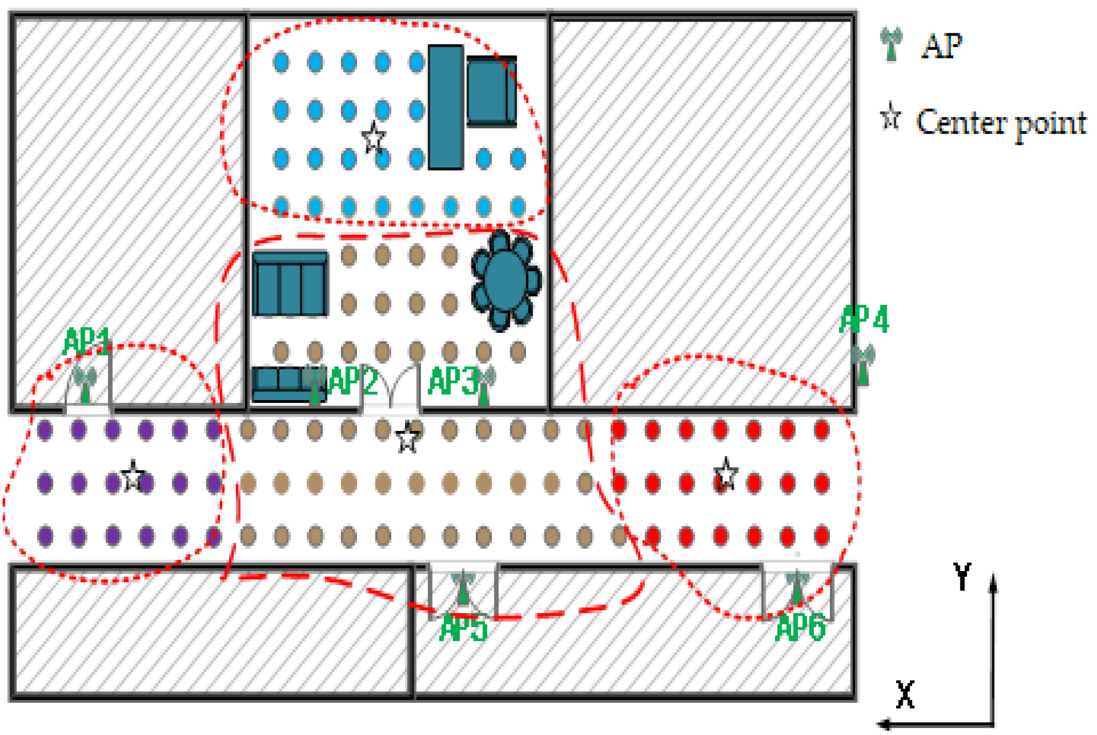
In a hierarchical clustering algorithm, the number of clusters L will affect the quality of the clustering results and ultimately affect the positioning accuracy. Thus, setting an appropriate number of clusters L is necessary. Based on the experimental results obtained in Section 3.1, we choose six APs (AP1, …, AP6) as the Wi-Fi RSSI signal APs and use the coverage area of the APs as the experimental area. In addition, we choose 122 reference fingerprint points (red dots) in the experimental area, and the distance between the reference points is 0.8 m. An experimenter holds the standard mobile terminal in front of his/her chest, keeps the same height and direction and collects the Wi-Fi RSSI fingerprint data at each reference fingerprint point at a frequency of 30 s/time for 3 min. We average all the RSSI data collected from each AP to establish an offline fingerprint database. According to the established offline fingerprint database, we set L as 3, 4, 5, 6, 7 or 8 then introduce the BWP [23] index to judge whether the clustering result is good or bad. The experimental results are shown in Figure 7. We can conclude that when L = 4, the result is the best. Therefore, we divide the offline fingerprint database into four regions and calculate the clustering centres of each region. The final results of the regional division in the environment are presented in Figure 8.
The five-pointed star icons represent the centre position of each cluster. From right to left, the coordinates of the four centre positions are (2.05, 3.85), (2.86, 13.04), (2.00, 21.50) and (8.28, 14.16).
3.3. Hidden Layer Structure Setting
Setting the hidden layer structure of the BPNN model is one of the conditions for establishing a satisfactory WOA-BPNN calibration algorithm model. In this study, we set the number of hidden layers of the BPNN model as one or two layers. According to Equation (18), we determine the number of neurons in each hidden layer. When the number of hidden layers of the BPNN model is two, the number of neurons in the first hidden layer and second hidden layer is the same.
where represents the number of neurons in the hidden layer, represents the number of input layers, represents the number of output layers and R is a constant between 1–10. As both the number of neurons in the input layer and the output layer in this experiment are 1, and too many or too few neurons in the hidden layer will cause the over-fitting or under-fitting of the experimental data, thus we determined that the number of neurons ranges from 5 to 11.
To compare and analyse the influence of the different BPNN models on the final calibration effect of the WOA-BPNN calibration algorithm to select the optimal BPNN model for the subsequent indoor positioning experiment, we chose the 12 modelling points (as shown in Figure 4) and the best number of Wi-Fi APs (six APs: AP1~AP6) to build a stable WOA-BPNN model. Then, we conducted the experiment in the experimental area described in Section 3.2. In addition, we add 19 test fingerprint points (purple triangles), which are in the middle of the two reference points, to detect the positioning accuracy of the model. The distribution of the test fingerprint points is shown in Figure 9.
At the offline phase, we establish an offline fingerprint database according to the method described in Section 3.2. At the online phase, we hold two test mobile terminals, collect the Wi-Fi RSSI test fingerprint data at each test fingerprint point at a frequency of 30 s/time for 3 min, and average all the collected RSSI data of each AP as the test input data of the WOA-BPNN model. Then, according to the mobile terminal models, calling the corresponding model for the RSSI calibration to obtain the predicted output RSSI data after calibration.
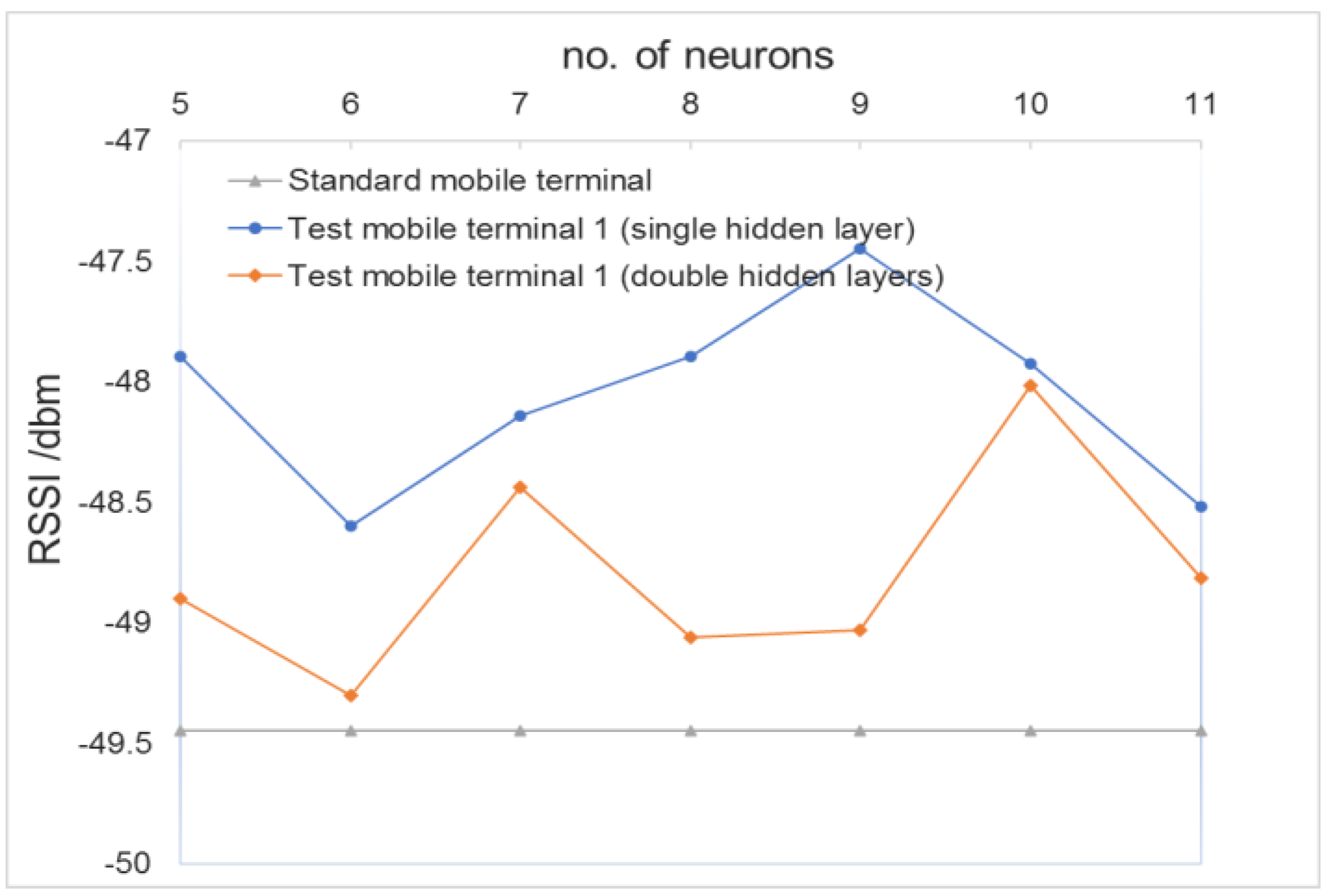
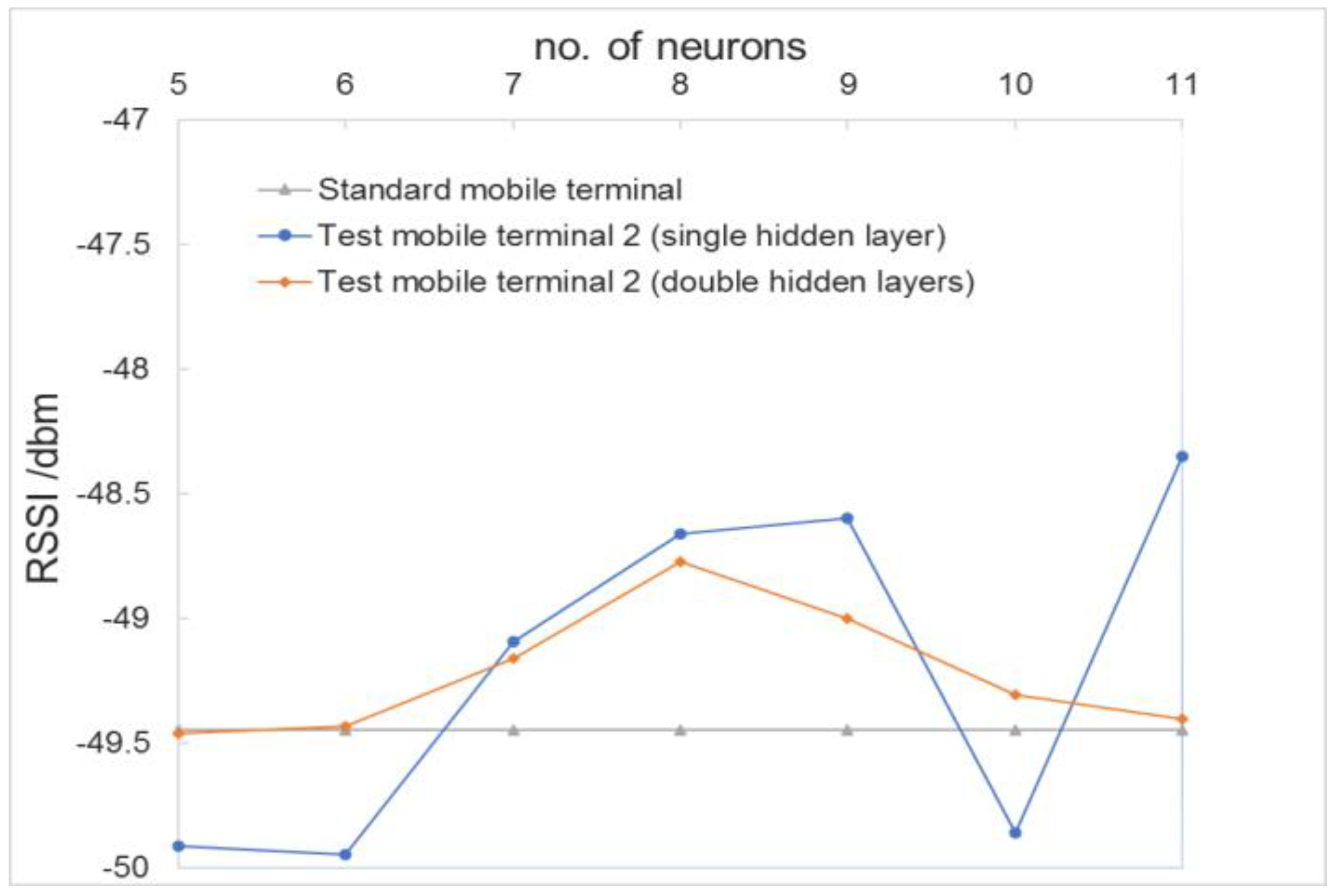
3.3.1. Influence of Hidden Layer Structure on Average RSSI Value
By changing the hidden layer structure of the BPNN model (e.g., the number of hidden layers or number of hidden layer neurons), we discuss the impact of the different BPNN model structures on the average RSSI results obtained after the calibration of the two test mobile terminals. Under different BPNN model structures we carried out five experiments to obtain the best calibration effect.
According to Figure 10 and Figure 11, for the two test mobile terminals, the BPNN model with double hidden layers can improve the calibration results of the WOA-BPNN calibration algorithm compared with the BPNN model with a single hidden layer. When the hidden layer structure of the BPNN model is double hidden layers and the number of neurons is six, the average RSSI error after the calibration is the smallest.
3.3.2. Influence of Hidden Layer Structure on Average Positioning Error
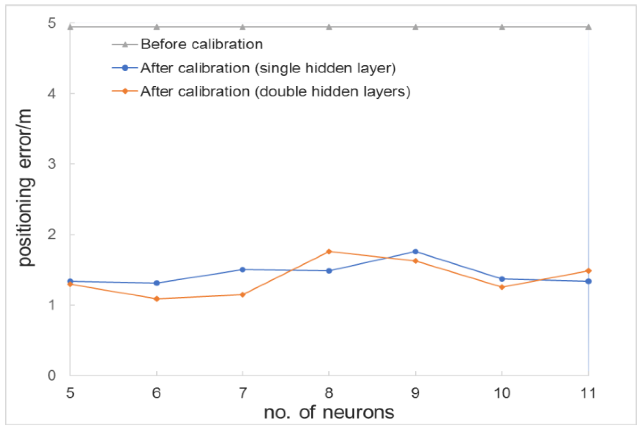
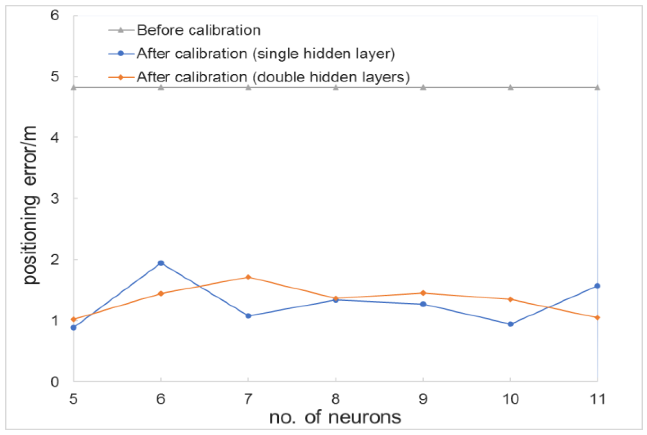
In this section, based on the five results of each BPNN model structure obtained in Section 3.3.1, we discuss the influence of the different BPNN model structures on the average positioning error results obtained after the calibration of the two test mobile terminals. The best positioning result of each BPNN model structure is shown in Figure 12 and Figure 13.
According to Figure 12 and Figure 13, for the two test mobile terminals, under the condition of the same number of neurons in each hidden layer, whether the hidden layer of the BPNN model is a single hidden layer or double hidden layers, the average positioning error reaches the minimum value when the number of neurons in the hidden layer is six and five, respectively.
It can be seen from the above results that more neurons in the hidden layer do not mean better WOA-BPNN calibration algorithm results. Therefore, based on the above results, and considering the problem of algorithm efficiency, we adopt the BPNN model with double hidden layers and six neurons in each hidden layer for the subsequent experiments.
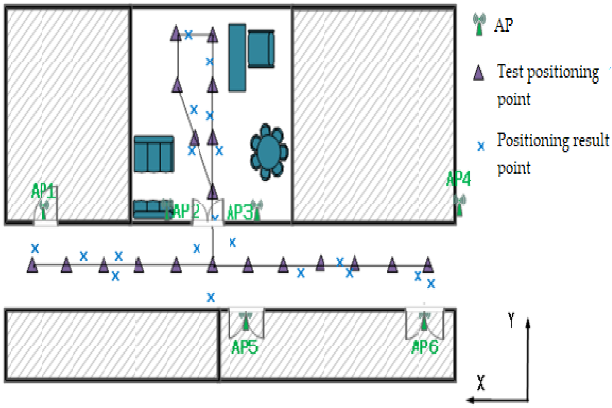
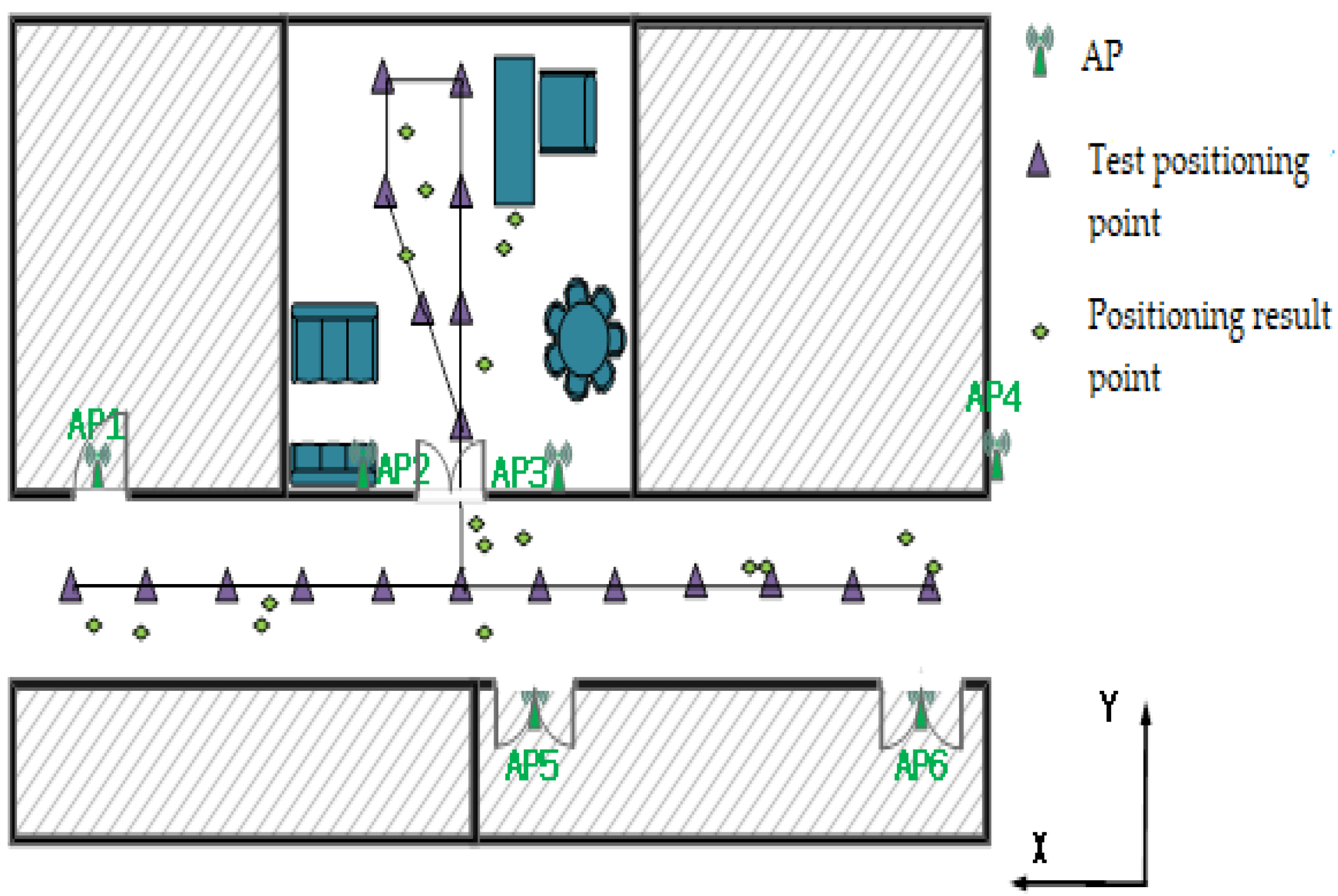
3.4. Trajectory Positioning Points
Based on the WOA-BPNN model established in the Section 3.3, and after processing the real-time positioning results of the two test mobile terminals, their trajectory positioning points are shown in Figure 14 and Figure 15.
4. Discussion
4.1. Comparison with Other Positioning Algorithms
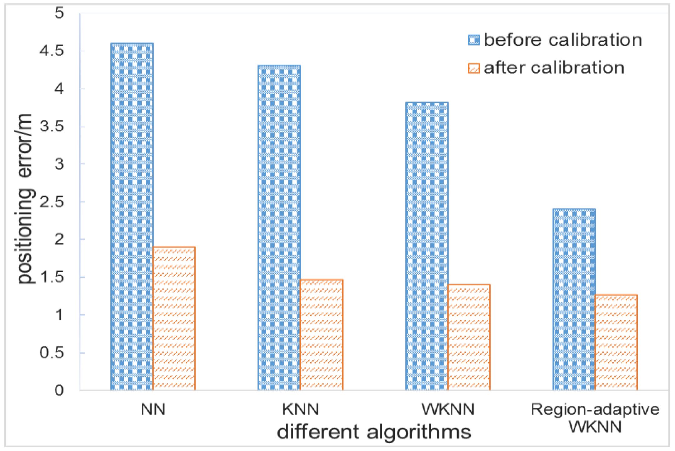
To verify the effectiveness of the WOA-BPNN calibration algorithm proposed in this study, we utilise four positioning algorithms, namely NN, KNN, WKNN and the proposed region-adaptive WKNN, to compare the average positioning error results before and after calibration with the WOA-BPNN calibration algorithm. Figure 16 shows the comparison of the average positioning error of the different positioning algorithms. It can be seen from Figure 16 that based on the proposed WOA-BPNN calibration algorithm, the average positioning error obtained by the above four positioning algorithms after calibration is much lower than the uncalibrated average positioning error. Among the algorithms, the proposed region-adaptive WKNN algorithm obtains the best result. Thus, we can conclude that the combination of the proposed WOA-BPNN calibration algorithm and proposed region-adaptive WKNN algorithm can effectively eliminate the heterogeneous differences in software and hardware in different mobile terminals to improve indoor positioning accuracy.
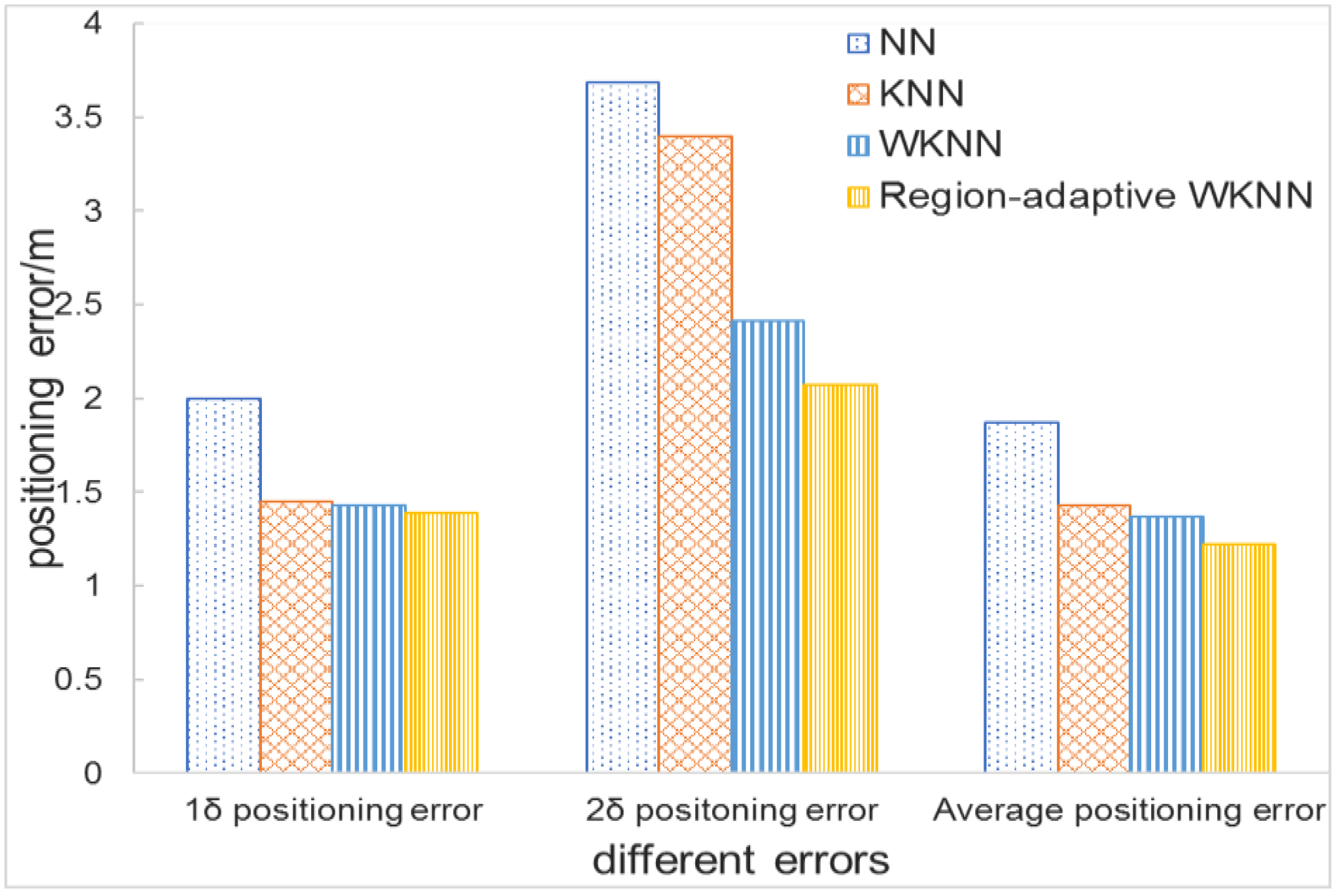
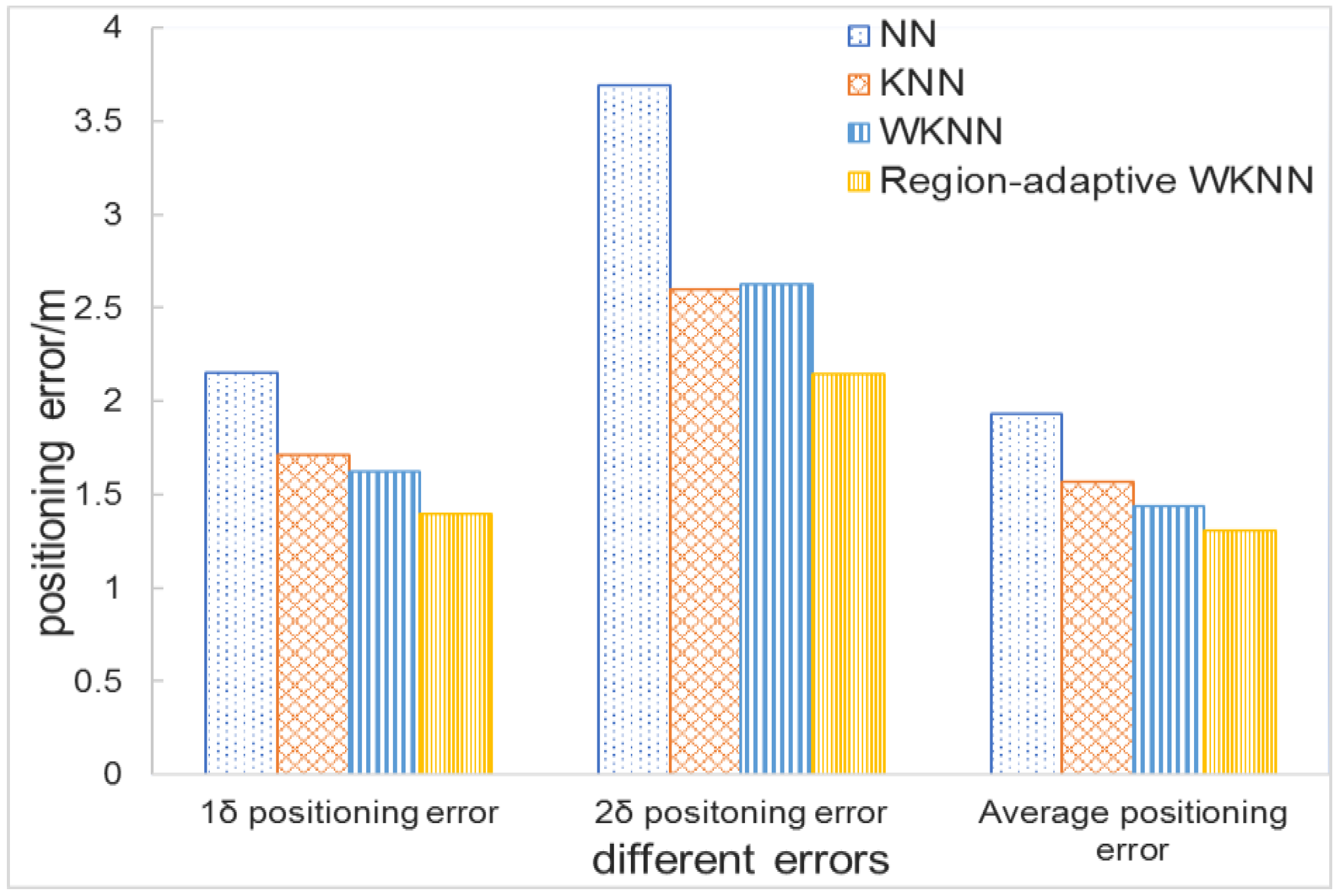
Meanwhile, to verify the effectiveness of the proposed region-adaptive WKNN algorithm based on hierarchical clustering, we also compare the different positioning errors of the four positioning algorithms based on the WOA-BPNN calibration algorithm, and the results are shown in Figure 17 and Figure 18. From the figures, we can see that under the one-sigma positioning error, the positioning error of test mobile terminal 1 using the proposed hierarchical clustering adaptive WKNN positioning method is about 0.61 m lower than that of the test mobile terminal using the NN positioning algorithm. In addition, the positioning error of test mobile terminal 2 using the proposed method is about 0.76 m, 0.31 m and 0.22 m lower than that of the test mobile terminal using the NN, KNN and WKNN positioning algorithms, respectively. Under the two-sigma positioning error, the positioning error of test mobile terminal 1 is reduced by about 1.62 m, 1.33 m and 0.34 m compared with that of the test mobile terminal using NN, KNN and WKNN positioning algorithms, respectively. In addition, the positioning error of test mobile terminal 2 is reduced by about 0.76 m, 0.31 m and 0.22 m compared with that of the test mobile terminal using the NN, KNN and WKNN algorithms, respectively. Under the average positioning error, the positioning error of test mobile terminal 1 and test mobile terminal 2 using the proposed positioning method is 1.22 m and 1.31 m, respectively, and the comprehensive average error can reach 1.27 m, which is about 0.64 m, 0.24 m and 0.14 m lower than that of the three other positioning algorithms. Moreover, the average positioning accuracy of the proposed algorithm is about 33%, 16% and 10% higher than that of the NN, KNN and WKNN positioning algorithms, respectively. Thus, it can be seen that under the three types of positioning error, the proposed method is better than the other positioning algorithms.
4.2. Comparison with Other Calibration Algorithms
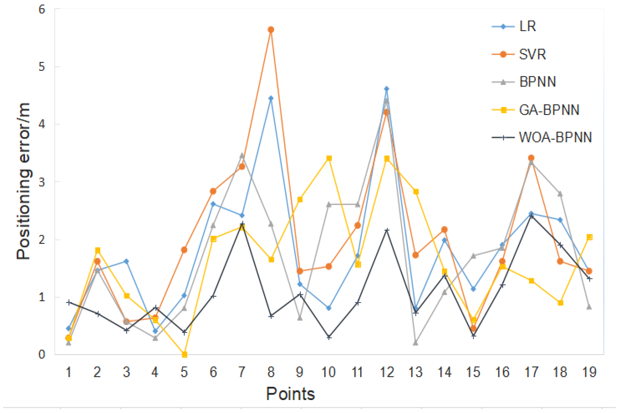
To verify the effectiveness of the proposed WOA-BPNN calibration algorithm, we compare the calibration positioning points generated by the LR, SVR, BPNN and GA-BPNN algorithms with those generated by the WOA-BPNN algorithm in real positioning points and obtain the positioning error of each positioning point, as shown in Figure 19. Moreover, in the tests, we set the one-sigma positioning error and two-sigma positioning error based on the ISO/IEC18305 international standard as the evaluation index and calculate the positioning error of the different mobile terminals using the different calibration algorithms, as shown in Table 1.
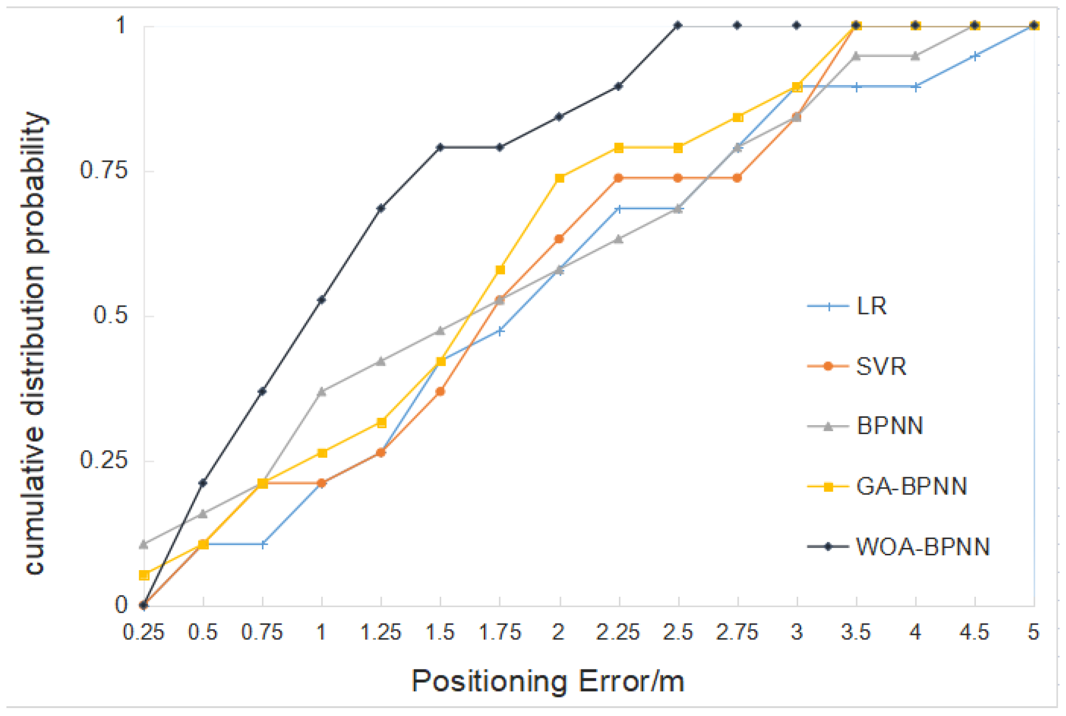
It can be seen from the table that the proposed WOA-BPNN calibration algorithm can effectively reduce the indoor positioning error. In this experiment, compared with the one-sigma positioning error of different mobile terminals using the LR, SVR, BPNN and GA-BPNN calibration algorithms, the one-sigma positioning error of the mobile terminals using the proposed WOA-BPNN calibration algorithm is reduced by 41%, 42%, 44% and 36% on average. In addition, the proposed WOA-BPNN calibration algorithm reduces the two-sigma positioning error of the mobile terminals by 37%, 25%, 26% and 17% on average, compared with the four other algorithms. These results effectively show that the proposed WOA-BPNN calibration algorithm is more accurate and feasible than the other calibration algorithms. Moreover, it can be seen from the cumulative distribution function of the positioning error in Figure 20 that the proposed calibration algorithm is better than the four other algorithms. Therefore, the field test results demonstrate that the proposed algorithm can effectively reduce the positioning error caused by the heterogeneity of mobile terminals and improve indoor positioning accuracy, thereby further improving the availability of positioning algorithms between different mobile terminals.
5. Conclusions
Firstly, focusing on the problem of the heterogeneity of software and hardware in different mobile terminals, we propose an indoor Wi-Fi RSSI calibration algorithm based on a WOA-BPNN. We use the WOA to find the optimal initial weights and thresholds of the BPNN, which addresses the drawback of the BPNN model falling easily into the local optimum. By applying a nonlinear convergence factor a, we further improve the convergence speed of the optimisation algorithm. The proposed calibration algorithm is simple to operate for handheld mobile terminals. We also compare the impact of the different structures of the BPNN model on the final calibration effect of the WOA-BPNN calibration algorithm. The experimental results show that the BPNN model with double hidden layers is more beneficial to the calibration effect of the algorithm than the BPNN model with a single hidden layer. Moreover, the test results suggest that a larger number of neurons in the hidden layer of the BPNN model do not directly lead to better calibration results by the WOA-BPNN calibration algorithm, because too many neurons in the hidden layer will lead to over-fitting in the network [11]. Secondly, to solve the problem of the low positioning accuracy of location fingerprint indoor positioning algorithms based on Wi-Fi RSSI, we propose a region-adaptive WKNN positioning algorithm based on hierarchical clustering. Finally, we further combine the WOA-BPNN calibration algorithm (where the hidden layer of the BPNN model is double layers, and the number of neurons in each layer is six) with region-adaptive WKNN position algorithm based on hierarchical clustering. Compared with the one-sigma positioning error of the different mobile terminals using the LR, SVR, BPNN and GA-BPNN calibration algorithms, the one sigma positioning error of the mobile terminals using the proposed WOA-BPNN calibration algorithm is reduced by 41%, 42%, 44% and 36% on average. In addition, the proposed WOA-BPNN calibration algorithm reduces the two-sigma positioning error of the mobile terminal by 37%, 25%, 26% and 17% on average, compared with the four other calibration algorithms. Thus, the proposed WOA-BPNN calibration algorithm can effectively reduce the indoor positioning error caused by the heterogeneity of software and hardware in different mobile terminals and improve the availability and universality of the positioning algorithm.
Author Contributions
M.Y. and L.C. guided the research work, supervised and organized the paper writing; X.W. and S.Y. conceived and designed the methodology and experiments; X.W. and S.Y. performed the experiments, analysed the data and wrote the paper; M.Y. and L.C. revised and submitted the paper. All authors have read and agreed to the published version of the manuscript.
Funding
This research was funded by the Program of the Ministry of Science and Technology, under Project application No.: S2022QYCXH0051.
Institutional Review Board Statement
Not applicable.
Informed Consent Statement
Not applicable.
Data Availability Statement
Not application.
Acknowledgments
We would like to express our heartfelt thanks to anonymous reviewers and editors for their constructive comments on the paper.
Conflicts of Interest
The authors declare no conflict of interest.
Nomenclature
| Symbol | Meaning |
| a | convergence factor |
| t | the current number of iterations of the whale population |
| tmax | the maximum number of iterations of the whale population |
| the initial weight | |
| the initial threshold | |
| the whale group position | |
| N | the size of whale population |
| T | the current number of iterations of the BPNN model |
| Tmax | the maximum number of iterations of the BPNN model |
| the fitness function | |
| the number of samples | |
| yi | the real value of the ith RSSI |
| y | the predicted value of the ith RSSI |
| A | one of the whale position parameters |
| C | one of the whale position parameters |
| r | a random value of [0, 1] |
| p | a random probability |
| the current whale position | |
| the optimal whale position | |
| the position of the whale at the next moment | |
| the distance between the current position and the optimal position | |
| b | a constant, which defines the logarithmic spiral shape |
| l | a random value in [–1, 1] |
| the randomly selected position of a whale | |
| the optimal weight and threshold of the BPNN model | |
| the connection weight between the neuron i and the neuron j | |
| the threshold of the neuron j | |
| the input value of the neuron j | |
| the output value of the neuron j | |
| the input value of the neuron i | |
| the loss function of the current iteration number | |
| the real output value of the output layer neuron j | |
| the predicted output value of the output layer neuron j | |
| the updated weight between the neuron i and the neuron j | |
| the updated threshold of the neuron j | |
| the learning rate between 0–1 | |
| D | the Euclidean distance between the RSSI of the real-time position and the RSSI of the class centre point F |
| rssij | the RSSI value of the jth Wi-Fi AP collected in real-time position |
| RSSImj | the RSSI value of the jth Wi-Fi AP of the centre point m of class |
| n | the number of Wi-Fi APs |
| (x1, y1) | the corresponding two-dimensional coordinates of the fingerprint points |
| di | the distance from the nearest neighbor point to other fingerprint points |
| the average distance from the nearest neighbor point to other fingerprint points | |
| S | the standard deviation from the nearest neighbor point to other fingerprint points |
| p | the error reduction ratio |
| the error between RSSI value of the test mobile terminal and that of the standard mobile terminal before calibration | |
| the error between the RSSI value of the test mobile terminal after calibration and that of the standard mobile terminal | |
| the number of error reduction after calibration in the test data | |
| Z | the total number of test data sets, which is proportional to the number of APs |
| L | the number of clusters |
| the number of neurons in the hidden layer | |
| the number of neurons in the input layer | |
| the number of neurons in the output layer | |
| a constant between 1–10 |
References
- Machaj, J.; Brida, P.; Piché, R. Rank based fingerprinting algorithm for indoor positioning. In Proceedings of the 2011 International Conference on Indoor Positioning and Indoor Navigation, Guimaraes, Portugal, 21–23 September 2011; pp. 1–6. [Google Scholar]
- Li, Z.; Liu, J.; Yang, F.; Niu, X.; Li, L.; Wang, Z.; Chen, R. A Bayesian Density Model Based Radio Signal Fingerprinting Positioning Method for Enhanced Usability. Sensors 2018, 18, 4063. [Google Scholar] [CrossRef] [PubMed] [Green Version]
- He, S.; Chan, S.; Lei, Y. SLAC: Calibration-Free Pedometer-Fingerprint Fusion for Indoor Localization. IEEE Trans. Mob. Comput. 2018, 17, 1176–1189. [Google Scholar] [CrossRef]
- Yang, L.; Liu, Q.; Xu, J.; Hu, J.; Song, T. An Indoor RFID Location Algorithm Based on Support Vector Regression and Particle Swarm Optimisation. In Proceedings of the 2018 IEEE 88th Vehicular Technology Conference (VTC-Fall), Chicago, IL, USA, 27–30 August 2018; pp. 1–6. [Google Scholar]
- Song, B.; Yu, M.; He, X. An Indoor Location WIFI Calibration Method Based on BP Neural Network. J. Navig. Position. 2019, 7, 43–47. [Google Scholar]
- Yu, Z.; Lu, X.; Tao, X. RSSI Ranging Algorithm Based on GA-BP Neural Network Model. J. Navig. Position. 2020, 8, 63–68. [Google Scholar]
- Ferreira, D.; Souza, R.; Carvalho, C. QA-kNN: Indoor Localization Based on Quartile Analysis and the kNN Classifier for Wireless Networks. Sensors 2020, 20, 4714. [Google Scholar] [CrossRef] [PubMed]
- Xue, W.; Hua, X.; Li, Q.; Qiu, W.; Peng, X. Improved Clustering Algorithm of Neighboring Reference Points Based on KNN for Indoor Localization. In Proceedings of the 2018 Ubiquitous Positioning, Indoor Navigation and Location-Based Services (UPINLBS), Wuhan, China, 22–23 March 2018; pp. 1–4. [Google Scholar]
- Zhao, H.; Huang, B.; Jia, B. Applying kriging interpolation for WiFi fingerprinting based indoor positioning systems. In Proceedings of the 2016 IEEE Wireless Communications and Networking Conference, Doha, Qatar, 3–6 April 2016; pp. 1–6. [Google Scholar]
- Li, J.; Gao, X.; Hu, Z.; Wang, H.; Cao, T.; Yu, L. Indoor Localization Method Based on Regional Division with IFCM. Electronics 2019, 8, 559. [Google Scholar] [CrossRef] [Green Version]
- He, C.; Guo, S.; Wu, Y.; Yang, Y. A Novel Radio Map Construction Method to Reduce Collection Effort for Indoor Localization. Measurement 2016, 94, 423–431. [Google Scholar] [CrossRef]
- Karsoliya, S. Approximating number of hidden layer neurons in multiple hidden layer BPNN architecture. Int. J. Eng. Trends Technol. 2012, 3, 714–717. [Google Scholar]
- Selami, Y.; Lv, N.; Tao, W.; Yang, H.; Zhao, H. Optimizing laser triangulation displacement sensor of 3D positioning and posture using COA Based BPNN. Sens. Rev. 2020, 40, 112–120. [Google Scholar] [CrossRef]
- Hu, J.; Wu, Z.; Qin, X.; Geng, H.; Gao, Z. An Extended Kalman Filter and Back Propagation Neural Network Algorithm Positioning Method Based on Anti-lock Brake Sensor and Global Navigation Satellite System Information. Sensors 2018, 18, 2753. [Google Scholar] [CrossRef] [PubMed] [Green Version]
- Xing, S.; Zhang, H.; Liang, X.; Gulliver, A. A 60 GHz impulse radio positioning algorithm based on a BP neural network. In Proceedings of the 2017 IEEE Pacific Rim Conference on Communications, Computers and Signal Processing (PACRIM), Victoria, BC, Canada, 21–23 August 2017; pp. 1–5. [Google Scholar]
- Mirjalili, S.; Lewis, A. The Whale Optimisation Algorithm. Adv. Eng. Softw. 2016, 95, 51–67. [Google Scholar] [CrossRef]
- Shaun, C.; Cedric, L. The Structure of Dark Matter Haloes in Hierarchical Clustering Models. Mon. Not. R. Astron. Soc. 1995, 281, 716–736. [Google Scholar]
- Long, W.; Jiao, J.; Liang, X.; Tang, M. An Exploration-enhanced Grey Wolf Optimiser to Solve High-dimensional Numerical Optimisatin. Eng. Appl. Artif. Intell. 2018, 68, 63–80. [Google Scholar] [CrossRef]
- Wang, W.; Tang, R.; Li, C.; Liu, P.; Luo, L. A BP Neural Network Model Optimised by Mind Evolutionary Algorithm for Predicting the Ocean Wave Heights. Ocean Eng. 2018, 162, 98–107. [Google Scholar] [CrossRef]
- Zhang, L.; Sun, Z.; Zhang, C.; Dong, F.; Wei, P. Numerical Investigation of the Dynamic Responses of Long-Span Bridges with Consideration of the Random Traffic Flow Based on the Intelligent ACO-BPNN Model. IEEE Access 2018, 6, 28520–28529. [Google Scholar] [CrossRef]
- Elaziz, M.A.; Mirjalili, S. A Hyper-heuristic for Improving the Initial Population of Whale Optimisation Algorithm. Knowl. Based Syst. 2019, 172, 42–63. [Google Scholar] [CrossRef]
- Lei, Y.; Yan, C.; Renu, S.; Belay, A. A modified WKNN indoor Wi-Fi localization method with differential coordinates. In Proceedings of the 2017 International Conference on Applied System Innovation (ICASI), Sapporo, Japan, 13–17 May 2017; IEEE: Piscataway, NJ, USA, 2017; pp. 1822–1824. [Google Scholar]
- Zhou, S.; Xu, Z.; Tang, X. Method for Determining the Optimal Cluster Number of K-means Algorithm. J. Comput. Appl. 2010, 30, 1995–1998. [Google Scholar]
Figure 1.
RSSI received by different mobile terminals in the same direction at the same position at the same time.
Figure 1.
RSSI received by different mobile terminals in the same direction at the same position at the same time.

Figure 2.
The calibration model of WOA-BPNN.

Figure 3.
The algorithm steps for the region-adaptive WKNN algorithm based on hierarchical clustering.
Figure 3.
The algorithm steps for the region-adaptive WKNN algorithm based on hierarchical clustering.

Figure 4.
Distribution of modelling points.

Figure 5.
Distribution of test points.

Figure 6.
Error reduction ratio for the number of Wi-Fi APs.

Figure 7.
The number of clusters L and the corresponding BWP results.

Figure 8.
Results of regional division.

Figure 9.
Distribution of test fingerprint points.

Figure 10.
Comparison of the average RSSI value after calibration of test mobile terminal 1.

Figure 11.
Comparison of the average RSSI value after calibration of test mobile terminal 2.

Figure 12.
Comparison of average positioning error before and after calibration of test mobile terminal 1.
Figure 12.
Comparison of average positioning error before and after calibration of test mobile terminal 1.

Figure 13.
Comparison of average positioning error before and after calibration of test mobile terminal 2.
Figure 13.
Comparison of average positioning error before and after calibration of test mobile terminal 2.

Figure 14.
Schematic diagram of track points of test mobile terminal 1 positioning results.

Figure 15.
Schematic diagram of track points of test mobile terminal 2 positioning results.

Figure 16.
Comparison of average positioning error of different positioning algorithms before and after calibration.
Figure 16.
Comparison of average positioning error of different positioning algorithms before and after calibration.

Figure 17.
Comparison of different errors of different algorithms after calibration. (Testing mobile terminal 1).
Figure 17.
Comparison of different errors of different algorithms after calibration. (Testing mobile terminal 1).

Figure 18.
Comparison of different errors of different algorithms after calibration. (Testing mobile terminal 2).
Figure 18.
Comparison of different errors of different algorithms after calibration. (Testing mobile terminal 2).

Figure 19.
Comparison of positioning error of different algorithms.

Figure 20.
Cumulative distribution function (CDF) of positioning error.


Table 1.
Comparison of positioning error of five calibration algorithms (m).
| Algorithms | LR | SVR | BPNN | GA-BPNN | WOA-BPNN | ||
|---|---|---|---|---|---|---|---|
| Indicator | |||||||
| Mobile Terminal | |||||||
| Test mobile terminal 1 | positioning error(one sigma) | 1.71 | 1.81 | 1.84 | 1.65 | 1.02 | |
| positioning error (two sigma) | 4.44 | 3.26 | 3.45 | 3.40 | 2.27 | ||
| Test mobile terminal 2 | positioning error (one sigma) | 2.24 | 2.21 | 2.34 | 2.00 | 1.32 | |
| positioning error (two sigma) | 3.49 | 3.41 | 3.29 | 2.61 | 2.72 | ||
Publisher’s Note: MDPI stays neutral with regard to jurisdictional claims in published maps and institutional affiliations. |
© 2022 by the authors. Licensee MDPI, Basel, Switzerland. This article is an open access article distributed under the terms and conditions of the Creative Commons Attribution (CC BY) license (https://creativecommons.org/licenses/by/4.0/).
Share and Cite
MDPI and ACS Style
Yu, M.; Yao, S.; Wu, X.; Chen, L. Research on a Wi-Fi RSSI Calibration Algorithm Based on WOA-BPNN for Indoor Positioning. Appl. Sci. 2022, 12, 7151. https://doi.org/10.3390/app12147151
AMA Style
Yu M, Yao S, Wu X, Chen L. Research on a Wi-Fi RSSI Calibration Algorithm Based on WOA-BPNN for Indoor Positioning. Applied Sciences. 2022; 12(14):7151. https://doi.org/10.3390/app12147151
Chicago/Turabian StyleYu, Min, Shuyin Yao, Xuan Wu, and Liang Chen. 2022. "Research on a Wi-Fi RSSI Calibration Algorithm Based on WOA-BPNN for Indoor Positioning" Applied Sciences 12, no. 14: 7151. https://doi.org/10.3390/app12147151
Note that from the first issue of 2016, this journal uses article numbers instead of page numbers. See further details here.