Time-Weighted Community Search Based on Interest

Abstract

Community search aims to provide users with personalized community query services. It is a prerequisite for various recommendation systems and has received widespread attention from academia and industry. The existing literature has established various community search models and algorithms from different dimensions of social networks. Unfortunately, they only judge the representative attributes of users according to the frequency of attribute keywords, completely ignoring the temporal characteristics of keywords. It is clear that a user’s interest changes over time, so it is essential to select users’ representative attributes in combination with time. Therefore, we propose a time-weighted community search model (TWC) based on user interests which fully considers the impact of time on user interests. TWC reduces the number of query parameters as much as possible and improves the usability of the model. We design the time-weighted decay function of the attribute. We then extract the user’s time-weighted representative attributes to express the user’s short-term interests more clearly in the query window. In addition, we propose a new attribute similarity scoring function and a community scoring function. To solve the TWC problem, we design and implement the Local Extend algorithm and the Shrink algorithm. Finally, we conduct extensive experiments on a real dataset to verify the superiority of the TWC model and the efficiency of the proposed algorithm.

1. Introduction

Community is the basis for various recommendation applications, such as friend recommendation, precision marketing, and activity organization [1,2,3,4]. Compared with community detection, community search can better explain the reasons for the formation of the community by personalized search according to the query criteria specified by the user. Therefore, community search has attracted extensive attention in academia and industry. Many query models and algorithms have emerged to serve various query scenarios.

Unfortunately, the existing models [2,3,4,5] do not fully describe users, especially their representative attributes (including text and spatial attributes). Take the geographic social network Foursquare as an example: it consists of millions of nodes, where each node represents a user, and an edge represents the friendship between two users. Users check in at different times and places. To make the query closer to reality, we should describe users based on multiple dimensions, such as spatial distance, social relations, interest attributes, and time. However, these models only judge the representative attributes of users according to the frequency of keywords. It is worth emphasizing that time plays an extremely important role in establishing social networks. The time change of users’ check-in records can best reflect their real interest trends. Especially in the recommendation system, we are more concerned with the short-term interests of users. The more recent the attributes are, the stronger the ability to represent users’ current interests, and the greater the weight that should be assigned. Therefore, selecting representative attributes only according to the frequency of keywords is inappropriate.

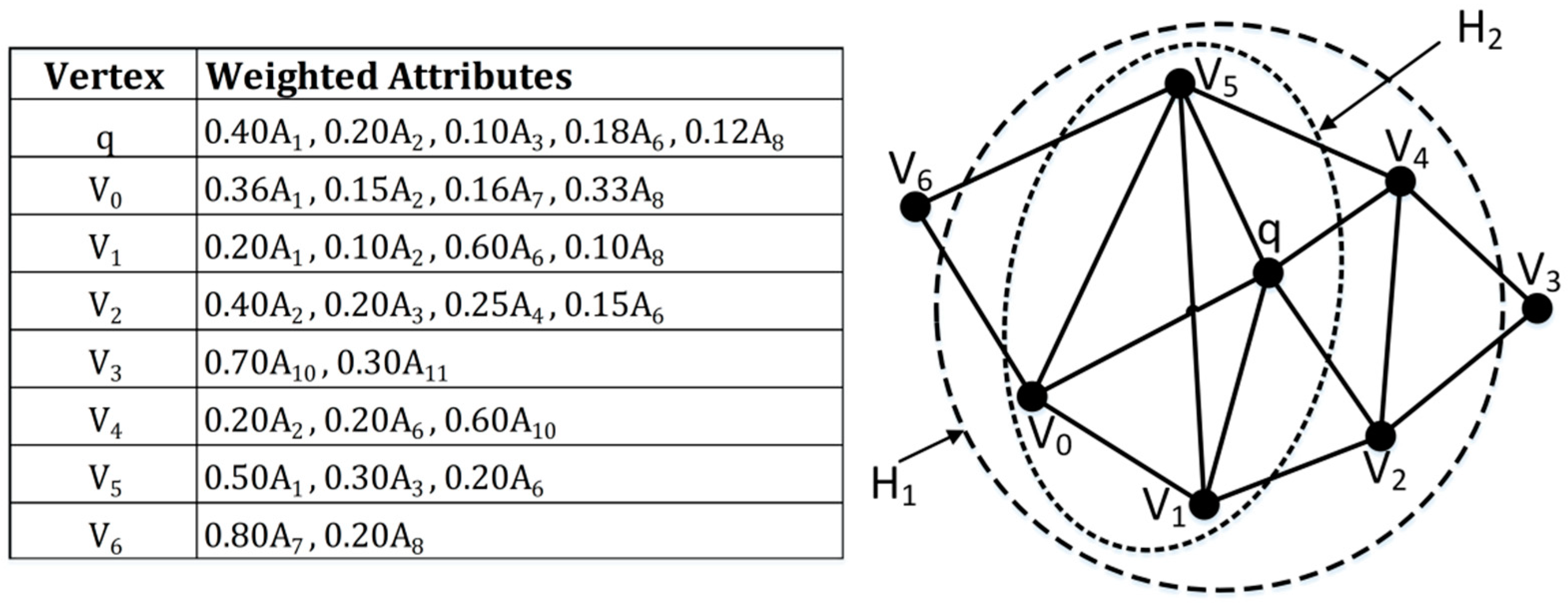
To alleviate the query dilemma caused by incomplete query dimensions and harsh query conditions, we propose a new community search model—Time-Weighted Community Search Based on Interest (TWC). When a user wants to find friends with interests similar to their own recent interests to form a community, TWC can provide efficient queries. TWC comprehensively considers the impact of space, structure, text, and time on the community and requires as few parameters as possible to start the query. Specifically, given a geographic social network graph, a query vertex, and a positive integer, TWC aims to find a subgraph—that is, a connected k-core—with the highest attribute similarity score. TWC does not require users to specify query keywords, avoiding low-quality communities caused by inappropriate keywords. It extracts representative attributes from users’ historical records and better explains the reasons for the formation of the community. At the same time, we calculate their weights based on the check-in time and frequency of the attributes. On this basis, a new node similarity scoring function and a subgraph scoring method are designed. In this article, we assume that the greater the attribute weight, the stronger the ability to represent users’ current interests. Figure 1 shows an example of a social network diagram and the weighted attribute list of nodes.

Our main contributions are as follows:

(1)

Fully considering the characteristics of geographic social networks, we propose a new community search model, Time-Weighted Community Search Based on Interest (TWC), by considering the four dimensions of structural cohesiveness, spatial cohesiveness, interest, and time.

(2)

We design the attribute time-weighted decay function and then extract the user’s time-weighted representative attributes, which express the user’s interest trend clearly in the query window. In addition, we propose a new attribute similarity scoring function and a community scoring function.

(3)

In order to solve the TWC problem, we design a Local Extend algorithm from inside to outside and a Shrink algorithm from outside to inside to deal with different search scenarios.

(4)

We carry out many experiments on the real dataset. Comparison with similar algorithms shows that the community nodes of TWC are similar to the current interests of query points and can better express the short-term interests of query users.

2. Related Work

Community search was originally designed to organize a cocktail party [1] with a good atmosphere. It organized a temporary community, and each user in the community was familiar with at least k users. Unlike community detection, community search can complete queries online through various index structures to improve efficiency. The existing community search models can be roughly divided into the following categories according to different evaluation dimensions.

(1) Community search based on structural cohesion and spatial cohesion

These kinds of community search models [2,3,4,5,6,7,8,9] are usually applied to simple graphs without considering the textual attributes of vertices. They aim to find a group of vertices that meet specific structural cohesion metrics and are close to each other to form a community. SSGQ [2] looks for a spatially aware community to reduce traffic time to the specifying aggregation. The vertices in the community form a k-core, and the distance to the aggregation place is the smallest. To find a group of users geographically close to each other, [5] used MCC to represent the minimum wrapping circle of the community. Under the same structural cohesion, the target community’s MCC is the smallest. In order to find more compact communities, [7] proposed a (k, d)-MCC search model, which requires that nodes meet the k-core and that the distance is not more than d.

(2) Community search based on structural cohesion and text attribute relevance

These search models perform community searches on attribute graphs, and it is worth noting that they are different from the traditional spatial keyword search [10,11]. The spatial keyword search in [12] aims to find vertices containing query keywords and returns them in the form of a tree. However, the community search model in [13,14,15] returns a subgraph, requiring that the subgraph nodes satisfy specific text attribute similarities metrics and contain the query vertices. The ACQ model [14] searches for an optimal community such that the nodes form as a k-core and share the most keywords with the query keywords set. Unfortunately, it treats all keywords equally, ignoring differences in weight. The community search in [15] employs (k-d)-truss as the structural cohesiveness metric, includes query vertexes, and requires that the distance from each node to the vertex set does not exceed d hops. Compared with [14], ATC believes that vertex attributes should own different weights related to the frequency of occurrence. However, unfortunately, it still ignores the influence of time on attribute weights. Therefore, ATC cannot be directly applied to solve the TWC problem.

(3) Community search based on structural cohesion and hybrid similarity

Hybrid similarity means that both spatial similarity and text attribute similarity are met simultaneously [16,17,18]. For example, the target communities of the ACOC model in [16] should contain all query keywords in the query attribute set. In addition to satisfying the k-core metric, the diameter of the community induced by these vertices should be minimal. ACOC has strict requirements for query parameters, which may result in an empty community. Although the VAC model [18] does not require users to specify query keywords, the application scenarios of VAC and TWC are different. VAC does not consider the impact of time on user interest. In addition, VAC’s scoring function is different from TWC and does not highlight the decisive role of the query node in the composition of the community. We will make a specific comparison in the experimental part.

Interest drift means that users’ interests change over time, which is the basis of this paper. Scholars have proposed various methods to model user interest drift and applied them to multiple recommendation scenarios [19,20,21,22]. In [20], they employed the time decay function to model user behavior and proposed an adaptive collaborative filtering method to predict the user’s future interest. The forgetting curve function has been used in a personalized recommendation system to model user interest [22]. The more recent the transaction time, the greater the user’s interest, which is consistent with the original intention of our paper. However, the model [22] cannot be used to solve the TWC problem. Firstly, the application of the forgetting curve in [22] is not comprehensive because it ignores the enhancement of user interest by repeated check-in. In addition, the decay granularity in [22] is rough. It treats the item as a whole and considers users as similar only when they interact with the same item. However, different items may share common keywords. Although users interact with different projects, they may be similar. Therefore, we choose to model keywords which can better describe users’ interests. In the experimental part, we compared the overlapping communities found in literature [22], which proved that the application of forgetting curve in TWC is more appropriate.

3. Problem Formulation

The problem we aim to solve is defined on an undirected, unweighted geographic social attribute network $G=\left(V,E\right)$, where $V$ is the vertex set and $E$ is the edge set. For each vertex $v\in V$, it has a text attribute set $A\left(v\right)$, and a location $P\left(v\right)=(P_x\left(v\right),P_y\left(v\right))$, where $P_x\left(v\right)$ and $P_y\left(v\right)$ denote its latitude and longitude coordinates in a two-dimensional space. For any subgraph $H=\left(V_H,E_H\right)\subseteq G$, $V_H\subseteq V \mathrm{and} E_H\subseteq E$ are maintained.

Table 1. Notations and meanings.

Notation	Meaning
$G=\left(V,E\right)$	a graph with vertex set $V$ and edge set $E$
$H\subseteq G$	$H$ is a subgraph of $G$, and $V_H$ and $E_H$ are the vertex set and edge set of $H$, respectively
$de{g}_H\left(v\right)$	the degree of vertex $v$ in $H$
AvgDegree($H$)	the average degree of nodes in graph $H$
$T_j$	a check-in timestamp
$A\left(v\right)=\left\{A_1\left(v\right),A_2\left(v\right),\dots ,A_l\left(v\right)\right\}$	text attribute set of node $v$
$W\left(v\right)=\left\{W_1\left(v\right),W_2\left(v\right),\dots ,W_l\left(v\right)\right\}$	attribute weight set of node $v$, ${\displaystyle \sum }_{i=1}^l{W}_i\left(v\right)=1$
$l=\left|A\left(v\right)\right|$	size of attribute set $A\left(v\right)$
$A\left(u,v\right)=A\left(u\right)\cup A\left(v\right)$	union of attribute sets $A\left(u\right)$ and $A\left(v\right)$ without duplicate attributes
$Vec\left(v\right)=\left(Ve{c}_1\left(v\right),Ve{c}_2\left(v\right),\dots ,Ve{c}_{l\_dimen}\left(v\right)\right)$	attribute weight vector of $A\left(u,v\right)$
$l\_dimen=\left|A\left(u,v\right)\right|$	size of attribute set $A\left(u,v\right)$
$P\left(v\right)=(P_x\left(v\right),P_y\left(v\right))$	position of node $v$, and $P_x\left(v\right)$, $P_y\left(v\right)$ are $v$’s latitude and longitude coordinates
$P_j\left(v\right)=\left(P_{xj}\left(v\right), P_{yj}\left(v\right)\right)$	check-in coordinates of node $v$ at $T_j$, and $P_{xj}\left(v\right), P_{yj}\left(v\right)$ are $v$’s latitude and longitude at $T_j$
$CosTime\left(u,v\right)$	the textual similarity score of node $u$ and $v$
$GSim\left(u,v\right)$	the spatial similarity score of node $u$ and $v$
$TScore(q,v)$	the similarity score of node$v$ and $q$
$TScore(q,H)$	the graph score of $H$ containing $q$
$r$	the time decay factor
$\alpha$	the balance factor of different type of attribute scores

shows the notations used in this paper.

Before formally formulating our problem, we first introduce the structure cohesiveness metric, the attribute time-weighted decay function, and the attribute similarity scoring function used in this paper.

3.1. Structure Cohesiveness

The commonly used structural cohesion matrices include k-clique, k-truss, and k-core. Due to its fast calculation and wide applications, we adopt k-core as a structural cohesion matric in this paper. However, k-core is not always connected, so we only consider the connected k-core as a community.

Definition 1.

(Connected k-core) Given a graph$G$and a non-negative integer$k$, a connected k-core is a connected subgraph$H$of graph$G$, where$\forall v\in E_H, de{g}_H\left(v\right)\ge k$.

In our algorithm, k-core can be easily replaced by other structural cohesion indicators to meet the structural requirements of different scenarios.

3.2. Time-Weighted Decay Function

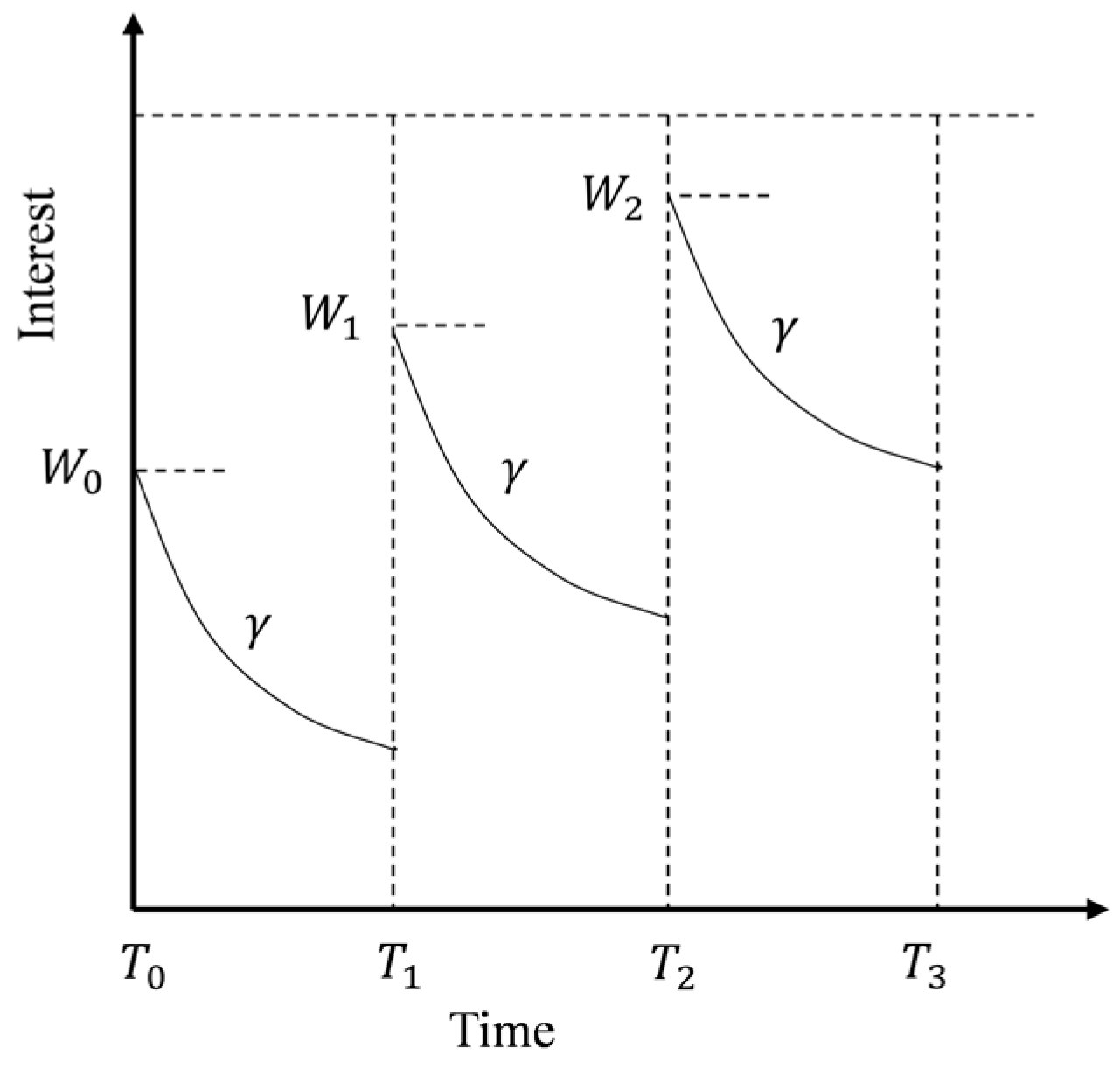
Intuitively, users’ interests change over time, and the more recent the attribute, the more representative it is, as with the location attributes. In addition, the higher the attribute frequency, the stronger the ability to express interest. The user’s interest in attributes is the largest at check-in and then decays at a certain speed. As shown in Figure 2, assuming that attribute $A_i\left(v\right)$ appears in $v$’s check-in records at $T_0$, $T_1$ and $T_2$, the user $v$’s interest in $A_i\left(v\right)$ is enhanced every time. This is consistent with the law of human memory, known as the Ebbinghaus memory curve.

Let $\gamma$ be the decay factor, representing the decay rate of interest. The larger the $\gamma$, the faster the attenuation. To simplify subsequent operations, let $\gamma$ remain constant at each check-in. We designed decay functions for single check-in and repeated check-in occasions of attributes, as shown in Formulas (1)–(3).

$$f\left(A_i\left(v\right), T_j\right)=e^{-r\Delta t_j}$$

(1)

$$f\left(A_i\left(v\right)\right)={\displaystyle \sum }_{j=0}^{N_v^i}f\left(A_i\left(v\right), T_j\right)$$

(2)

$$W_i\left(v\right)=\frac{f\left(A_i\left(v\right)\right)}{{{\displaystyle \sum }}_{m=1}^{l}f\left(A_m\left(v\right)\right)}$$

(3)

Formula (1) expresses the attenuation of user $v$’s interest in $A_i\left(v\right)$ from time $T_j$, where $\Delta t_j=\frac{T_{end}-T_j}{T_{end}-T_{start}}$, $T_j$ is the check-in time of $A_i\left(v\right)$, and $T_{start} \mathrm{and} T_{end}$ are the start and end timestamps of the whole query window. As can be seen from Formula (1), the fresher the $T_j$ is, the smaller the $\Delta t_j$ and the larger the $f\left(A_i\left(v\right), T_j\right)$, indicating that the user is more interested in the attribute $A_i\left(v\right)$. Since $A_i\left(v\right)$ may appear in several check-in records at different times $T_j$, Formula (2) describes $v$’s overall interest in $A_i\left(v\right)$, where $N_v^i$ is the sum of the occurrence times of $A_i\left(v\right)$ in the historical check-in records of user $v$. For the convenience of comparison, we normalize $v$’s interest in all attributes and finally obtain the weight of attribute $A_i\left(v\right)$ named as $W_i\left(v\right)$, which is $v$’s interest in attribute $A_i\left(v\right)$. The larger the $W_i\left(v\right)$, the greater the user $v$’s interest in $A_i\left(v\right)$. Note that ${\displaystyle \sum }_{i=1}^l{W}_i\left(v\right)=1$.

Ebbinghaus memory curve is also applicable to users’ spatial attributes. Assuming that the check-in location of user $v$ at $T_j$ is $P_j\left(v\right)=\left(P_{xj}\left(v\right), P_{yj}\left(v\right)\right)$ and they have checked in $N$ times in the whole history query window, the spatial position after weighted attenuation integration is shown in Formulas (4) and (5).

$$P_x\left(v\right)={\displaystyle \sum }_{j=0}^N{e}^{-r\Delta t_j}{P}_{xj}\left(v\right)$$

(4)

$$P_y\left(v\right)={\displaystyle \sum }_{j=0}^N{e}^{-r\Delta t_j}{P}_{yj}\left(v\right)$$

(5)

Here, $\Delta t_j=\frac{T_{end}-T_j}{T_{end}-T_{start}}$, $r$ is the decay factor, the same as in Formula (1). The more recent the coordinates, the stronger the ability to represent the user’s current position. Figure 1 shows nodes’ text attributes and their corresponding weights, which is the basis of node similarity evaluation.

3.3. Attributes Similarity Scoring Function

We evaluate the similarity between users from two aspects: text attributes and spatial attributes. For text attribute similarity, Jaccard similarity is usually preferred, which means that the more attributes shared between two nodes there are, the more similar they are. Nevertheless, Jaccard similarity treats all attributes equally, ignoring the corresponding weights, which is inconsistent with the problem studied in our paper. Therefore, we design an improved cosine similarity method to measure their textual similarity.

Let $A\left(u\right)=\left\{A_1\left(u\right),A_2\left(u\right),\dots ,A_{l_1}\left(u\right)\right\}$ and $A\left(v\right)=\left\{A_1\left(v\right),A_2\left(v\right),\dots ,A_{l_2}\left(v\right)\right\}$ be the attribute set of $u$ and $v$, where $l_1$ does not have to equal $l_2$. Their corresponding weights are $W\left(u\right)=\left\{W_1\left(u\right),W_2\left(u\right),\dots ,W_{l_1}\left(u\right)\right\}$ and $W\left(v\right)=\left\{W_1\left(v\right),W_2\left(v\right),\dots ,W_{l_2}\left(v\right)\right\}$. In order to compare the similarity of node attributes in the same dimensions, we integrate their attribute sets as $A\left(u,v\right)=A\left(u\right)\cup A\left(v\right)=\left\{A_1\left(u,v\right),A_2\left(u,v\right),\dots ,A_{l\_dimen}\left(u,v\right)\right\}$, where $l\_dimen=\left|A\left(u,v\right)\right|$, representing the size of the attribute set $A\left(u,v\right)$ without duplicate attributes. Then, taking $A\left(u,v\right)$ as the metric space, we design the attribute weight vector of node $v$ as $Vec\left(v\right)=\left(Ve{c}_1\left(v\right),Ve{c}_2\left(v\right),\dots ,Ve{c}_{l\_dimen}\left(v\right)\right)$. For attribute weight vector $Vec\left(v\right)$, if $A_i\left(u,v\right)\in A\left(v\right), i=1,\dots ,l\_dimen$, make $Ve{c}_i\left(v\right)=W_i\left(v\right)$, otherwise $Ve{c}_i\left(v\right)=0$. We construct the vector $Vec\left(u\right)=\left(Ve{c}_1\left(u\right),Ve{c}_2\left(u\right),\dots ,Ve{c}_{l\_dimen}\left(u\right)\right)$ in the same way. When comparing with different users, the attribute weight vector of $v$ may be different due to the different metric space. Now, we define the text attribute similarity function of node $u$ and $v$ as

$$CosTime\left(u,v\right)=\frac{Vec\left(u\right)·Vec\left(v\right)}{\Vert Vec\left(u\right)\Vert \Vert Vec\left(v\right)\Vert }$$

(6)

where $Vec\left(u\right)$ and $Vec\left(v\right)$ are the attribute weight vector of node $u$ and $v$, and $Vec\left(u\right)·Vec\left(v\right)$ represents the dot product of $Vec\left(u\right)$ and $Vec\left(v\right)$, $\Vert Vec\left(u\right)\Vert$ and $\Vert Vec\left(v\right)\Vert$ are the lengths of $Vec\left(u\right)$ and $Vec\left(v\right)$. The more shared attributes and the greater the weight of shared attributes, the more similar they are in textual attributes.

As shown in Figure 1, we take $q$ as the query node, $V_0$ and $V_1$ as candidate nodes, and then calculate the similarity with $q$. If Jaccard is employed, $Jaccard\left(q,V_0\right)=0.5$,$Jaccard\left(q,V_1\right)=0.8$, and $V_1$ should be the target node. However, the weights of shared attributes in $q$ are small, which can not sufficiently represent $q$’s interests.

When we take $CosTime$ as the similarity function, $CosTime\left(q,V_0\right)=0.787$, $CosTime\left(q,V_1\right)=0.67$, then $V_0$ should be selected due to the shared attributes’ own larger weights, and they are more suitable to describe $q$’s short-term interests.

For spatial attributes, we adopt Euclidean distance to measure the spatial similarity of nodes. Given the nodes’ locations according to Formula (4) and (5), we define their spatial similarity as

$$GSim\left(u,v\right)=\frac{1}{1+dist\left(u,v\right)}$$

(7)

where $dist\left(u,v\right)$ is the Euclidean distance between $u$ and $v$. Obviously, the greater the distance, the lower the similarity. To comprehensively evaluate various attributes, we employ parameter $\alpha$ to balance text attributes and spatial attributes. Then, the similarity of nodes is

$$TScore\left(u,v\right)=\alpha CosTime\left(u,v\right)+\left(1-\alpha \right)GSim\left(u,v\right)$$

(8)

Note that $CosTime\left(u,v\right)\in \left[0,1\right]$, $GSim\left(u,v\right)\in \left[0,1\right]$, so $TScore\left(u,v\right)\in \left[0,1\right]$. In this paper, we assume that the greater the $TScore\left(u,v\right)$, the higher the similarity. Based on the attribute similarity of nodes, we define the score of the graph as follows.

Definition 2.

(Attribute similarity score of the graph) Given a subgraph$H\subseteq G$and a query node$q$, the attribute similarity score of$H$is expressed as$TScore(q,H)$, which is the minimum value of the similarity scores between$q$and all others nodes in$H$—that is,$TScore(q,H)=\underset{v\in V_H}{min}TScore\left(q,v\right)$.

We formally define the time-weighted community search (TWC) based on user interest, as shown below.

Problem 1.

(TWC-problem) Given an attributed graph $G=\left(V,E\right)$, a query node $q$, and a non-negative integer $k$, the time-weighted community search based on user’s interest can return a subgraph $H\subseteq G$, satisfying the following conditions:

(1)

Connectivity: $H$ is a connected graph containing $q$.

(2)

Structure cohesiveness: $\forall v\in H, de{g}_H\left(v\right)\ge k$.

(3)

Attribute score maximum: While satisfying (1) and (2), the attribute similarity score of $H$,$TScore(q,H)$, is the highest, where $TScore(q,H)=\underset{v\in V_H}{\min }TScore\left(q,v\right)$.

(4)

There does not exist another subgraph $H^{\prime }\supseteq H$ satisfying the above three properties.

We re-observe Figure 1 and let $q$ be the query vertex, $k=3$. Since $TScore(q,H_1)=0.226<TScore(q,H_2)=0.67$ and a 4-core subgraph does not exist, we select $H_2=\left\{q,v_0,v_1,v_5\right\}$ as the optimal solution.

4. Methods

In order to solve the TWC problem, we designed a Local Extend algorithm and a Shrink algorithm. Before introducing the specific algorithm, we first explain the concept of feasible community.

Definition 3.

(Feasible Community) A subgraph$H\subseteq G$is a feasible community of TWC, only if$H$is a connected$k-core$, containing the query node$q$.

The feasible community meets the requirements (1) and (2) defined in TWC. A most intuitive method is finding all feasible communities, calculating their scores one by one, then selecting the community with the best score as the optimal solution for TWC. Unfortunately, this method is not suitable for large-scale social network graphs for its huge computational cost. Thus, we will no longer consider it.

4.1. Local Extend Algorithm

The intuitive algorithm is essentially the enumeration of graphs starting from $q$, resulting in massive invalid subgraphs. According to the nesting nature of k-core, we believe that if there is a better solution, it must be included by the initial feasible community. Therefore, we first detect the maximum feasible community $H$ as the initial subgraph, which can significantly reduce the search space. We calculate $TScore\left(q,v\right)$ for each node $v$ in $H$, then sort them in descending order according to the score. Starting from $q$, we gradually expand the nodes under the guidance of the best score until a feasible community is formed. Then, we choose the feasible community with the highest score, that is, the optimal solution. We use $Et$ to represent the extended point set, $C$ represents the candidate point set, $H_B$ represents the current optimal solution, and $H_{Et+v}$ represents the feasible solution derived from $Et+v$. During each expansion, we select the best node according to the following node selection strategy:

• Strategy 1: Select the neighbor node $v$ of $Et$ from $C$ with the highest $TScore(q,v)$;
• Strategy 2: If there are multiple nodes satisfying strategy (1), we choose the node with the largest degree.

Strategy 1 ensures that the score of the subgraph is monotonically decreasing. Strategy 2 is to select nodes with cohesive structures and organize them into feasible solutions as soon as possible. At the same time, we follow the following extension rules and stop rules.

• Extend Rule 1: If $TScore\left(q,H_{Et+v}\right)<TScore\left(q,H_B\right)$ and $\left|H_B\right|>\left|H_{Et+v}\right|$, then add node $v$ to $Et$ and continue to expand.
• Extend Rule 2: If $TScore\left(q,H_{Et+v}\right)>TScore\left(q,H_B\right)$, then add node $v$ to $Et$, update $H_B=H_{Et+v}$ and continue to expand.
• Extend Rule 3: If $TScore\left(q,H_{Et+v}\right)=TScore\left(q,H_B\right)$ and $\left|H_B\right|<\left|H_{Et+v}\right|$, then add node $v$ to $Et$, update $H_B=H_{Et+v}$ and continue to expand.

Extend Rule 1 describes the early stage of the algorithm, not finding enough nodes to form a feasible community. Extend Rule 2 shows that the addition of node $v$ allows us to obtain a new feasible solution with a higher score, and so we update the current optimal community. Extend Rule 3 occurs after Extend Rule 2. Adding a new best node $v$ does not reduce the score of $H_B$, indicating that the algorithm has found a larger feasible community and should update the current optimal solution.

• Stop Rule 1: If $TScore\left(q,H_{Et+v}\right)<TScore\left(q,H_B\right)$ and $H_B\subseteq H_{Et+v}$, then stop extension.
• Stop Rule 2: If $C=\varnothing$, then stop extension.

Stop Rule 1 may be triggered after the feasible solution is formed. Specifically, if $H_B$ cannot maintain its score when expanding $v$, we can conclude that there will not exist a more extensive feasible community whose score is no less than $H_B$. Thus, the expansion should be stopped and return $H_B$ as the optimal solution. Stop Rule 2 is easy to understand. There are no extensible nodes, so $H_B$ is naturally the optimal community.

The Local Extend algorithm is outlined in Algorithm 1, which integrates all expansion and stop strategies. In the worst case, the initial feasible solution is the optimal solution, and thus the algorithm will expand from $q$ to each node, but generally not.

Algorithm 1 Local Extend Algorithm $\left(G,q,k\right)$

Input: A graph $G=\left(V,E\right),$ a query node $q$, a non-negative integer $k.$ Output: A $k-core H_B$ with the maximum $TScore(q,H_B)$. 1: Find the maximum feasible community $H$ as initial subgraph. 2: For each node $v$ in $H,$ compute $TScore\left(q,v\right), \mathrm{then} \mathrm{arrange} \mathrm{them} \mathrm{in}$ descending order according to the score. 3: $Et\leftarrow q; C\leftarrow V_H-q; H_B\leftarrow H;$ 4: Extend ( $Et,C,H_B$ ) 5: return $H_B$. Procedure $\mathrm{Extend}\left(Et,C,H_B\right)$ 6: if $C=\varnothing$, then 7:            Update $H_B; \mathrm{over};$ 8: else 9:          Select the best node $v$ from $C$ according to the vertex selection strategy. 10:        if $TScore\left(q,H_{Et+v}\right)<TScore\left(q,H_B\right)$ and $\left|H_B\right|>\left|H_{Et+v}\right|$, then 11:                 $Extend\left(Et+v,C-v,H_B\right)$; 12:        else if $TScore\left(q,H_{Et+v}\right)>TScore\left(q,H_B\right)$ then 13:                 $H_B\leftarrow H_{Et+v}$; 14:                 $Extend\left(Et+v,C-v,H_B\right)$; 15:        else if $TScore\left(q,H_{Et+v}\right)=TScore\left(q,H_B\right)$ and $\left|H_B\right|<\left|H_{Et+v}\right|$, then 16:                   $H_B\leftarrow H_{Et+v}$; 17:                   $Extend\left(Et+v,C-v,H_B\right)$; 18:        else if $TScore\left(q,H_{Et+v}\right)<TScore\left(q,H_B\right) \mathrm{and} H_B\subseteq H_{Et+v}$, then 19:                  update $H_B;$ over.

We use the graph in Figure 1 to illustrate the Local Extend algorithm. We assume that $q$ is the query vertex and $k=3$.

Table 2. Illustration of Algorithm 1 on the graph in Figure 1.

Step	$\mathit{E}\mathit{t}$	$\mathit{C}$	${\mathit{H}}_{\mathit{E}\mathit{t}+\mathit{v}}$	${\mathit{H}}_{\mathit{B}}$
Step 1	$q$	$v_5,v_0,v_1,v_2,v_4$	$\varnothing$	$q,v_5,v_0,v_1,v_2,v_4$
Step 2	$q,v_5$	$v_0,v_1,v_2,v_4$	$\varnothing$	$q,v_5,v_0,v_1,v_2,v_4$
Step 3	$q,v_5,v_0$	$v_1,v_2,v_4$	$\varnothing$	$q,v_5,v_0,v_1,v_2,v_4$
Step 4	$q,v_5,v_0,v_1$	$v_2,v_4$	$q,v_5,v_0,v_1$	$q,v_5,v_0,v_1$
Step 5	$q,v_5,v_0,v_1,v_2$	$v_4$	$q,v_5,v_0,v_1,v_2$	$q,v_5,v_0,v_1$

shows the expansion process. Step 1–Step 3 follow Extend Rule 1. In Step 4, with the addition of node $v_1$, $TScore\left(q,H_{Et+v}\right)>TScore\left(q,H_B\right)$, the algorithm updates $H_B$ as $\left\{q,v_5,v_0,v_1\right\}$. In Step 5, the addition of node $v_2$ leads to the reduction in the score of the feasible algorithm $H_{Et+v}$, so the algorithm ends, and the optimal solution of TWC is $H_2=\left\{q,v_5,v_0,v_1\right\}$.

4.2. Shrink Algorithm

The closer the initial community is to the optimal solution, the less efficient the Local Extend algorithm is. In the worst case, it needs to traverse all nodes. In order to solve this query dilemma, we design a Shrink algorithm, which is also inspired by k-core nesting. Given an initial feasible community $H_B$, to obtain a better solution $H_B^{\prime }\subset H_B$, then we only need to delete some nodes $V_{H_B-H_B^{\prime }}$ from $H_B$. According to the definition of TWC, we can delete nodes that contribute less to the score of the subgraph without damaging the structure of the feasible community. As shown in Algorithm 2, the Shrink algorithm can be divided into three steps. First, we operate core decomposition and find the maximum k-core containing $q$ as the initial subgraph $H$ of the algorithm. Then, for each node $v$ in $H$, we calculate their similarity score $TScore\left(q,v\right)$ and sort them in ascending order according to the score. Finally, we delete nodes gradually until $H$ cannot be maintained as a feasible community and take the latest feasible solution as the optimal solution.

Algorithm 2 Shrink Algorithm $\left(G,q,k\right)$

Input: A graph $G=\left(V,E\right),$ a query node $q$, a non-negative integer $k.$ Output: A $k-core H_B$ with the maximum $TScore(q,H_B)$. 1: Find the maximum feasible community $H$ as initial subgraph. 2: Compute $TScore\left(q,v\right)$, form them as an ascending list $Sim\_list=\left\{\left(v,TScore\left(q,v\right)\right):\forall v\in H\right\}$. 3: Compute and form their core numbers as $Core\left(H\right)=\left\{\left(v,core\left(v\right)\right):\forall v\in H\right\}$. 4: while $H$ exists do 5:               $H_B \leftarrow H$; 6:              Select the first node $v$ in $Sim\_list$ as the node to be deleted. 7:              Delete $v$ and its incident edges from $H$; 8:              Delete $v$ from $Sim\_list$; 9:              Update $Core\left(H\right)$ with the core maintenance algorithm, and organize nodes as $Impossible=\{v:\forall v\in H \mathrm{and} core number core\left(v\right)<k\}$ 10:            For nodes in $Impossible$, remove them from $H$ and $Sim\_li\mathit{s}t$; 11:            Maintain $H$ as a feasible community; 12: Return the latest feasible community as $H_{\mathit{B}}.$

As shown in Algorithm 2, the Shrink algorithm maintains an ascending sequence of similarity. Deleting nodes one by one according to the order in $Sim\_list$ can gradually improve the score of feasible community and avoid blind trial and error. We note that deleting nodes may change the core numbers of their neighbors. Therefore, we employ the dynamic core maintenance algorithm proposed by [23] to update the core numbers, avoiding multiple global core decomposition. We record these nodes whose core number is less than $k$ during the core maintenance procedure and organize them as $Impossible$. Then, we remove them from $Sim\_list$, which can significantly shorten the length of $Sim\_list$ and stop the iteration as early as possible.

As shown in Figure 1, we initiate the query $Q=\left(G,q,3\right)$, and the initial feasible community is $H_1=\left\{q,v_4,v_2,v_1,v_0,v_5\right\}$. According to the Shrink algorithm, we first delete $v_4$, and then we observe that $\mathrm{core}\left(v_2\right)=2<k$, meaning $v_2$ will not appear in the final feasible community, so that we can remove $\left\{v_4,v_2\right\}$ from $Sim\_list$ together. After two iterations, the optimal solution found by the Shrink algorithm is $H_2=\left\{q,v_5,v_0,v_1\right\}$, which is the same as the Local Extend algorithm.

5. Results

In this part, we implement our proposed TWC model and the corresponding algorithm in Python and evaluate their effectiveness and efficiency. All experiments were conducted on a Linux Server with Intel Xeon CPU E5-2630 (2.2 GHz) and 125 GB memory.

We conducted all experiments on Foursquare [24], which includes long-term check-in data for about 22 months from Apr 2012 to Jan 2014, venue data, and friend relationship data. The dataset contains 22,809,624 check-ins by 114,324 users at 3,820,891 venues. Each row in the friend’s snapshot file indicates a friendship between two users. Each check-in record includes the user ID, venue ID, and check-in time. Each venue ID corresponds to several category keywords. If a user checks in at a venue, we believe that the user is interested in the attributes related to the venue ID. We note, however, that users may check-in at different venues, and different venues may have the same category of keywords. Therefore, we calculate the cumulative weight of attributes according to Formulas (1)–(3).

5.1. Case Study

Since VAC also adopts the idea of taking query points as the center, which is very similar to TWC, we first compare it with VAC. To fairly compare the two models, we first transform the VAC model into a k-core-based model and change the scoring function from distance to similarity: the more significant the similarity, the higher the score. We randomly select node $q$ as the query node, search communities using the DFS-based VAC algorithm and TWC’s Local Extend algorithm, respectively, and then compare the similarity between vertices and $q$. Taking node UserId = 769697 as query node $q$, we set $k$ = 10, α = 1, use VAC and TWC model to query, respectively, and record the queried communities as $H_{vac}$ and $H_{twc}$. Figure 3 shows the nodes in the community in terms of Jaccard similarity and CosTime similarity.

As shown in Figure 3a, the three nodes {‘1474184’, ‘639615’, ‘647188’} in $H_{vac}$ are abandoned by $H_{twc}$ because, although they have high Jaccard similarity with $q$, their CosTime similarity is relatively low—especially the node ‘647188’, which is significantly reduced. In other words, although they share many attributes with $q$, the related check-in record occurred a long time ago and cannot represent $q$’s current interests. We observe that $H_{twc}$ replaces them with five new nodes, {‘1190126’, ‘665064’, ‘1472376’, ‘1458831’, ‘1026751’}, as shown in Figure 3b. Although their Jaccard similarity with $q$ is low, the attributes they share with $q$ have a larger weight in $q$’s attributes set, which can better represent $q$’s current interests. This phenomenon proves that the more recent the shared attributes, the greater the similarity of users’ short-term interests. In terms of community score, $TScore\left(q,H_{vac}\right)=0.016$, $TScore\left(q,H_{twc}\right)=0.021$, and the score of $H_{twc}$ increased by 34% compared with $H_{vac}$. In addition, the community becomes more cohesive for AvgDegree ($H_{vac}$) = 10.6 and AvgDegree ($H_{twc}$) = 12.8. Therefore, by adopting the time-weighted decay function proposed in this paper to assign different weights to attributes and employing CosTime as the node similarity evaluation method, we can filter nodes more similar to $q$ and form a higher-quality community.

5.2. Effectiveness and Efficiency Evaluation of the Model

To evaluate the effectiveness of the TWC model on the attribute graph, we compare our Local Extend algorithm with the existing attribute-driven community search (ATC) [15], attributed community query (ACQ) [14], vertex-centric attributed community search (VAC) [18], and the time-weighted overlapping community detection (TWOD) [22]. We randomly selected 100 nodes as query nodes in each experiment and calculated the average value as the experimental result. It is worth noting that TWOD [22] is essentially a global community detection that cannot conduct personalized queries based on user-specified parameters. Therefore, we only compare the TWC and TWOD models from the perspective of user interest drift. In addition, each node may have multiple overlapping communities. For a fair comparison, we take the average value of all overlapping communities of the query node as the result of TWOD in each experiment.

• Experiment 1: time distribution of community shared attributes

For the community found in the model, we filter the keywords shared with $q$ and form them into a shared attribute set. We take the historical check-in time of $q$ as the time-effective window, take the latest check-in timestamp as the start of the window, and divide the time window into sub-windows with a proportion of 10%, 20%, 30%, 40%, and 50%. We calculate the proportion of shared keywords involved in the time window in the entire shared attribute set. As shown in

Table 3. The distribution proportion of community attributes in different time windows of $q$.

Time Effective Window	10% Window	20% Window	30% Window	40% Window	50% Window
TWC	0.115	0.237	0.478	0.686	0.814
ACQ	0.006	0.065	0.126	0.208	0.325
ATC	0.063	0.097	0.158	0.197	0.305
VAC	0.084	0.105	0.178	0.186	0.317
TWOD	0.075	0.122	0.207	0.297	0.496

, the digit in each cell represents the distribution proportion of the attributes in the shared attribute set in the current time window. Because the time window is divided in reverse order by timestamp, the larger the proportion in a smaller time window, the more recent the attribute is, and the closer the short-term interests of community members and the query node are.

It is not difficult to find that about 50% of the keywords shared by TWC communities appear in the first 30% of the time window, indicating that community members are closer to the short-term attributes of query node. Although TWOD applies the forgetting curve, the experimental results show that the proportion of shared keywords in the first 30% time window is only 20.7%. The reason is that TWOD ignores the enhancement effect of repeated check-in on user interest and does not consider the possibility that different items may share common keywords. The decay granularity is too rough, resulting in insufficient ability to express users’ short-term interests. Other models mainly use high-frequency words as the representative attribute of users, ignoring time, resulting in a low proportion of their shared attributes in the more recent time window, indicating that the current interests of community members and the query node are not well-matched.

• Experiment 2: community fitness comparison caused by interest drift

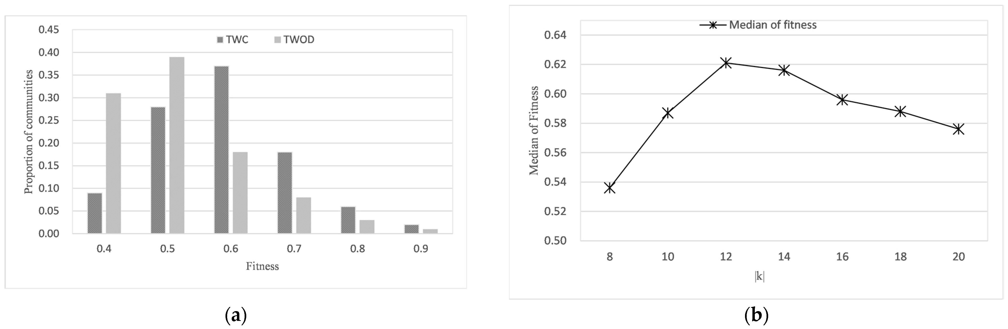
Because both TWOD and TWC adopt the forgetting curve to model users’ interests drift and similarities, they build different communities on this basis. We refer to the definition of fitness in [25] and design the fitness function of the community as follows.

$$fitness=\frac{w^{in}}{w^{in}+w^{out}}$$

(9)

where $w^{in}$ means the sum of the similarities of all paired nodes in the community, and $w^{out}$ represents the sum of the similarities between the community nodes and their direct external neighbors. For each query node, we first calculate the fitness of the queried community and then count the proportion of communities in different fitness intervals.

As shown in Figure 4a, the fitnesses of 83% of TWC communities vary in the range of 0.5~0.7, while the fitnesses of 70% of TWOD communities are in the range of 0.4~0.5. Only when two users check in the same project will the TWOD model think that the two users are similar; otherwise, the corresponding value in the user–user matrix is 0. However, friends may just check in for similar items, which leads to the user–user matrix failing to capture the real social relationship. Hence, the community’s fitness based on the user–user matrix is not high. TWC model is based on the social network snapshot, which reflects the real social relationship between users. In addition, the similarity between users is evaluated according to the historical occupancy records of users so that the community can be better divided. Since TWOD is not affected by k, we evaluate the change in the median fitness of the community queried by the TWC model at different k. As shown in Figure 4b, the community’s fitness increases with the growth of k and finally tends to be stable. Compared with k = 10, the fitness of the TWC model is better than that of TWOD.

• Experiment 3: the effect of k on effectiveness

Since TWOD is a global community detection, we will not compare it with other community search models. We gradually vary parameter k from 8 to 20 and compare the improvement of $H_{twc}$ in similarity score compared with $H_{vac}$. As shown in Figure 5a, no matter the value of k, the community score of $H_{twc}$ is better than that of $H_{vac}$. This is because the scoring function of TWC defines the decisive role of query nodes and selects nodes with high similarity in descending order, while the scoring function of VAC measures the similarity between all nodes, which undoubtedly weakens the leading role of query nodes. As k grows, the improvement tends to be stable. This is because the initial feasible community is smaller and more stable. The lowest similarity score determines the community score, and so the average similarity of the community also has the same trend.

• Experiment 4: the effect of query time window on effectiveness.

Let us set the whole record time of the dataset as a time window and the latest timestamp as the start of the window. In reverse order of time, five sub-windows are set, denoted as 20%, 40%, 60%, 80%, and 100% time windows, respectively. Then, we compare the improvement of $H_{twc}$ in similarity score compared with $H_{vac}$. As shown in Figure 5b, the improvement is not obvious when the time window is small. This is because the check-in records included are relatively few and fresh, so the difference in weights is not obvious. As the time window enlarges, more and more records are included in the calculation. The difference between attribute weights is gradually enlarged, which is more conducive to filtering out low-weight attributes. Hence, the score improvement is more obvious. However, the improvement is reduced when the time window is large enough, indicating that blindly expanding it is not appropriate because it will include the old and frequently occurring attributes in the user’s interest list and disperse the weight of these significant attributes.

• Experiment 5: the effect of k on efficiency.

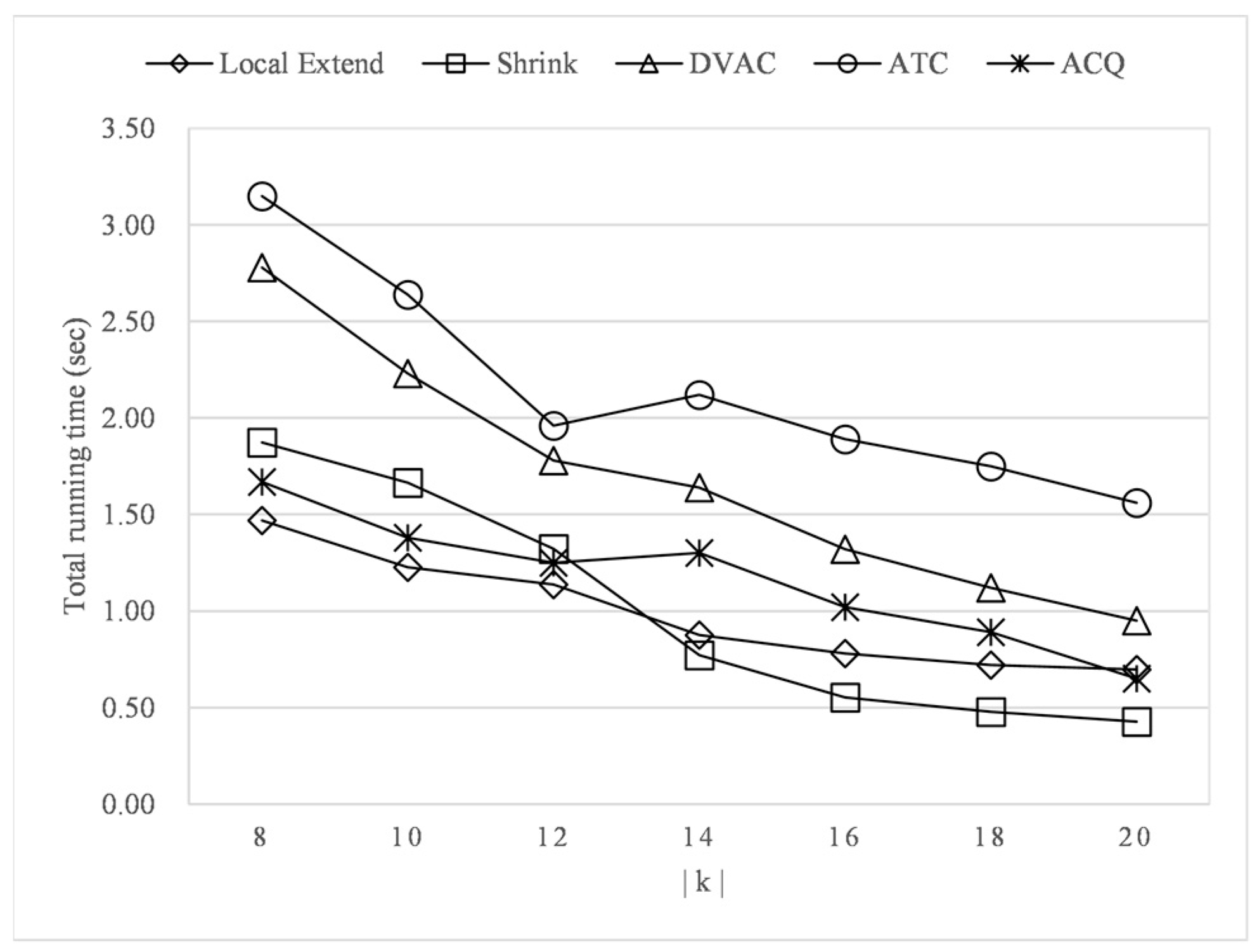
Since the efficiency of the TWC model is only affected by $k$, and the communities found by the Local Extend algorithm and the Shrink algorithm are the same, we vary k to compare the efficiency of different modes.

As shown in Figure 6, the community is large and incohesive enough when $k$ is small. The Local Extend algorithm expands the nodes from inside to outside in descending order of similarity, which can quickly form the optimal solution. Along with the increase in $k$, the initial feasible community becomes closer to the optimal community. Only a few nodes need to be deleted to build the optimal community. Therefore, the Shrink algorithm performs better than the Local Extend algorithm. At the same time, we note that no matter how the value of $k$ varies, the TWC model is faster than VAC and ATC. This is because the community score function of TWC only considers the similarity with the query node, while ATC and VAC consider all pairs of nodes, so their calculation is expensive. Since ACQ adopted k-core as the structural cohesion metric, it is faster than ATC and VAC. However, because the index construction takes a long time, ACQ has little difference from the efficiency of TWC.

6. Conclusions

In this paper, we study a new attributed community search problem named time-weighted community search (TWC) based on interest, which integrates time into community query. We design a time-weighted attribute weight decay function to find users’ representative attributes and design a new similarity scoring method. Two query methods are designed to solve the TWC problem, which can meet the query requirements in different scenes. Multiple experiments have proved that the communities discovered by the TWC model are more in line with the short-term interests of users.

References

- Sozio, M.; Gionis, A. The Community-Search Problem and How to Plan a Successful Cocktail Party. In Proceedings of the 16th ACM SIGKDD International Conference on Knowledge Discovery and Data Mining—KDD ’10, Washington, DC, USA, 25–28 July 2010; ACM Press: Washington, DC, USA, 2010; p. 939. [Google Scholar] [CrossRef]
- Yang, D.-N.; Shen, C.-Y.; Lee, W.-C.; Chen, M.-S. On Socio-Spatial Group Query for Location-Based Social Networks. In Proceedings of the 18th ACM SIGKDD International Conference on Knowledge Discovery and Data Mining—KDD ’12, Beijing, China, 12–16 August 2012; ACM Press: Beijing, China, 2012; p. 949. [Google Scholar] [CrossRef] [Green Version]
- Shen, C.-Y.; Yang, D.-N.; Huang, L.-H.; Lee, W.-C.; Chen, M.-S. Socio-Spatial Group Queries for Impromptu Activity Planning. IEEE Trans. Knowl. Data Eng. 2015, 28, 196–210. [Google Scholar] [CrossRef] [Green Version]
- Zhu, Q.; Hu, H.; Xu, C.; Xu, J.; Lee, W.-C. Geo-social group queries with minimum acquaintance constraints. VLDB J. 2017, 26, 709–727. [Google Scholar] [CrossRef]
- Fang, Y.; Cheng, R.; Li, X.; Luo, S.; Hu, J. Effective Community Search over Large Spatial Graphs. Proc. VLDB Endow. 2017, 10, 709–720. [Google Scholar] [CrossRef] [Green Version]
- Ghosh, B.; Ali, M.E.; Choudhury, F.M.; Apon, S.H.; Sellis, T.; Li, J. The Flexible Socio Spatial Group Queries. Proc. VLDB Endow. 2018, 12, 99–111. [Google Scholar] [CrossRef] [Green Version]
- Chen, L.; Liu, C.; Zhou, R.; Li, J.; Yang, X.; Wang, B. Maximum Co-Located Community Search in Large Scale Social Networks. Proc. VLDB Endow. 2018, 11, 1233–1246. [Google Scholar] [CrossRef] [Green Version]
- Fang, Y.; Wang, Z.; Cheng, R.; Li, X.; Luo, S.; Hu, J.; Chen, X. On Spatial-Aware Community Search. IEEE Trans. Knowl. Data Eng. 2019, 31, 783–798. [Google Scholar] [CrossRef]
- Zhang, F.; Zhang, Y.; Qin, L.; Zhang, W.; Lin, X. When Engagement Meets Similarity. Proc. VLDB Endow. 2017, 10, 998–1009. [Google Scholar] [CrossRef] [Green Version]
- Li, Y.; Wu, D.; Xu, J.; Choi, B.; Su, W. Spatial-aware interest group queries in location-based social networks. Data Knowl. Eng. 2014, 92, 20–38. [Google Scholar] [CrossRef]
- Guo, T.; Cao, X.; Cong, G. Efficient Algorithms for Answering the M-Closest Keywords Query. In Proceedings of the Acm Sigmod International Conference, Melbourne, VIC, Australia, 31 May–4 June 2015; pp. 405–418. [Google Scholar]
- FeLipe, I.D.; Hristidis, V.; Rishe, N. Keyword Search on Spatial Databases. In Proceedings of the IEEE 24th International Conference on Data Engineering, Cancun, Mexico, 7–12 April 2008. [Google Scholar]
- Zhang, Z.; Huang, X.; Xu, J.; Choi, B.; Shang, Z. Keyword-Centric Community Search. In Proceedings of the 2019 IEEE 35th International Conference on Data Engineering (ICDE), Macao, China, 8–11 April 2019; IEEE: Macao, China, 2019; pp. 422–433. [Google Scholar] [CrossRef]
- Fang, Y.; Cheng, R.; Luo, S.; Hu, J. Effective Community Search for Large Attributed Graphs. Proc. VLDB Endow. 2016, 9, 1233–1244. [Google Scholar] [CrossRef] [Green Version]
- Xin, H.; Lakshmanan, L. Attribute-Driven Community Search. Proc. VLDB Endow. 2017, 10, 949–960. [Google Scholar]
- Luo, J.; Cao, X.; Xie, X.; Qu, Q.; Xu, Z.; Jensen, C.S. Efficient Attribute-Constrained Co-Located Community Search. In Proceedings of the 2020 IEEE 36th International Conference on Data Engineering (ICDE), Dallas, TX, USA, 20–24 April 2020; IEEE: Dallas, TX, USA, 2020; pp. 1201–1212. [Google Scholar] [CrossRef]
- Chen, L.; Liu, C.; Zhou, R.; Xu, J.; Li, J. Finding Effective Geo-Social Group for Impromptu Activities with Diverse Demands. In Proceedings of the KDD ’20: The 26th ACM SIGKDD Conference on Knowledge Discovery and Data Mining, Virtual Event, CA, USA, 6–10 July 2020. [Google Scholar]
- Liu, Q.; Zhu, Y.; Zhao, M.; Huang, X.; Xu, J.; Gao, Y. VAC: Vertex-Centric Attributed Community Search. In Proceedings of the 2020 IEEE 36th International Conference on Data Engineering (ICDE), Dallas, TX, USA, 20–24 April 2020; IEEE: Dallas, TX, USA, 2020; pp. 937–948. [Google Scholar] [CrossRef]
- Lee, T.-Q.; Park, Y. A Time-Based Recommender System Using Implicit Feed-back. In CSREA EEE; Citeseer: Princeton, NJ, USA, 2006; pp. 309–315. [Google Scholar]
- Rafeh, R.; Bahrehmand, A. An Adaptive Approach to Dealing with Unstable Behaviour of Users in Collaborative Filtering Systems. J. Inf. Sci. 2012, 38, 205–221. [Google Scholar] [CrossRef]
- Sun, B.; Dong, L. Dynamic Model Adaptive to User Interest Drift Based on Cluster and Nearest Neighbors. IEEE Access 2017, 5, 1682–1691. [Google Scholar] [CrossRef]
- Feng, H.; Tian, J.; Wang, H.J.; Li, M. Personalized Recommendations Based on Time-Weighted Overlapping Community Detection. Inf. Manage. 2015, 52, 789–800. [Google Scholar] [CrossRef]
- Li, R.-H.; Yu, J.X.; Mao, R. Efficient Core Maintenance in Large Dynamic Graphs. IEEE Trans. Knowl. Data Eng. 2014, 26, 2453–2465. [Google Scholar] [CrossRef] [Green Version]
- Yang, D.; Qu, B.; Yang, J.; Cudre-Mauroux, P. Revisiting User Mobility and Social Relationships in LBSNs: A Hypergraph Embedding Approach. In Proceedings of the 2019 World Wide Web Conference, San Francisco, CA, USA, 13–17 May 2019. [Google Scholar]
- Lancichinetti, A.; Fortunato, S.; Kertesz, J. Detecting the Overlapping and Hierarchical Community Structure of Complex Networks. New J. Phys. 2009, 11, 033015. [Google Scholar] [CrossRef]
Figure 1.
Geographic social network graph.
Figure 2.
Interest decay curve caused by multiple check-ins.
Figure 3.
Comparison of community nodes queried by different models. (a) Nodes in community and their similarity with ; (b) nodes in community and their similarity with .
Figure 4.
Community fitness comparison. (a) Proportion of communities in different fitness ranges when k = 10; (b) median of community fitness with different k.
Figure 5.
Effectiveness evaluation of different models. (a) Change of similarity improve ratio with different k; (b) change of similarity improve ratio with different time windows.
Figure 6.
Efficiency evaluation of different models with different k.