Predictive Distillation Method of Anchor-Free Object Detection Model for Continual Learning

Abstract

Continual learning (CL) is becoming increasingly important, not only for storage space because of the ever-increasing amount of data being generated, but also for associated copyright problems. In this study, we propose ground truth’ (GT’), which is a combination of ground truth (GT) and a prediction of the teacher model that distills the prediction results of the previously trained model, called the teacher model, by applying the knowledge distillation (KD) technique to an anchor-free object detection model. Among all the objects predicted by the teacher model, an object for which the prediction score is higher than the threshold value is distilled into the current trained model, called the student model. To avoid interference with new class learning, the IoU is obtained between every object of the GT and the predicted objects. Through the continual learning scenario, even if the reuse of past data is limited, if new data are sufficient, the proposed model minimizes catastrophic forgetting problems and enables learning for newly added classes. The proposed model was learned in PascalVOC 2007 + 2012 and tested in PascalVOC2007, with better results of 9.6% p mAP and 13.7% p F1ⁱ shown in the scenario 19 + 1. The result in scenario 15 + 5 showed better results than the compared algorithm, with 1.6% p mAP and 0.9% p F1ⁱ. The scenario 10 + 10 also outperformed the other alternatives, with 0.9% p mAP and 0.6% p F1ⁱ.

1. Introduction

Compared to traditional computer vision algorithms, deep learning shows innovative performance, and it is accordingly being applied in a variety of fields. In areas where deep learning is successfully applied, the label of the data is completely defined before the deep learning model is learned, and the input, output, and internal layer structure of the model is fixed. In Chen and Liu’s ‘Life Machine Learning’ [1], this environment is called isolated learning, and the application of continual learning is stated to be essential for deep learning to develop in a manner similar to human intelligence. Human learning is a type of cumulative learning wherein what was previously learned in the learning process is not forgotten.

Assuming that the classification target is changed several times to re-learn the pre-learned deep learning model, most of the learned knowledge is forgotten and changed to suit the new target in the general learning paradigm process. Because the existing learning paradigm cannot accumulate what has been learned before, if re-learning is performed several times by changing the target, then the model will no longer be able to classify objects that have previously been well-classified. Continual learning (CL) is proposed to solve this problem and can be distinguished from other learning paradigms in that it accumulates previously learned knowledge so that it can be applied to constantly increasing classification targets [1,2,3,4].

The CL paradigm must simultaneously classify previous and current objects well while preventing the problem of forgetting previously learned knowledge. In the re-learning process, the problem of not being able to classify objects that were previously well-classified is called catastrophic forgetting. The main purpose of CL is to derive the minimum oblivion for all previously learned tasks and the maximum inference accuracy for new tasks [1,2].

In this study, we propose an object detection CL model that applies the knowledge distillation (KD) [5,6] method to minimize catastrophic forgetting. The object detection algorithm performs a task in which the name, location, and size of an object in an image are predicted simultaneously. Most object detection models in deep learning use anchor boxes to detect the size and location of objects. However, the problem with the anchor box is that it leads to more parameters, and therefore, a higher computational cost. Moreover, in a real-world environment, the object, size, and characteristics of continuously increasing data are not known in advance, so the anchor box is not suitable for CL. Therefore, the object detection model used in the proposed model is CenterNet [7], which is an anchor-free model that ensures a certain level of accuracy, even with a small number of parameters [8].

In KD, one of the types of algorithms for CL, the previously learned model is referred to as the teacher model (t-model), whereas the model that classifies the newly learned object is referred to as the student model (s-model). In general, object detection CL models using KD mainly employ the method of distilling a specific layer of the t-model in the s-model to minimize the differences between the two models [5,6].

Since CL research involves a very large range of scenarios and algorithms, the model proposed in this study has the following limitations and conditions.

• It targets class incremental learning (class IL) without a separate task ID.
• A scenario is set up assuming that data and labels cannot be reused.
• It targets CL models that do not store samples or feature maps of training data so that learning data cannot be estimated.
• The model structure is fixed to avoid increasing the parameters such that the inference time of the model does not increase.
• In the next training step, information on the previous class object can only be delivered using the weights of the previous learning model.
• Scenarios are pre-defined according to the order of CL learning.
• The object detection CL model proposed in this study is an algorithm for distilling the teacher model prediction (t-pred) and delivering it to the next learning model. This can be distinguished from the models described in prior studies in the following ways:
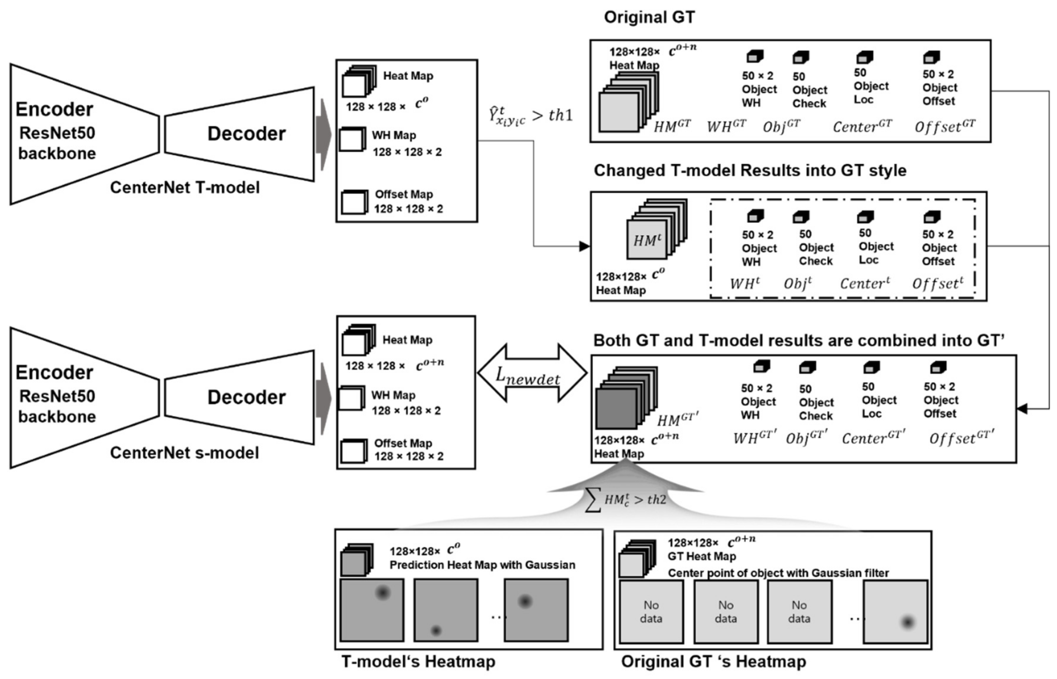
• Instead of the simple layer distillation KD technique, we propose a method for generating the GT’ that combines t-pred with the ground truth (GT), which transforms t-pred into the same form as the GT.
• Two problems of t-pred, the prediction result of the t-model, are solved as follows:
  • Not all results of t-pred are correct; to delete the error results, prediction information is only used when the prediction score of t-pred is greater than or equal to the threshold value.
  • Objects included in the GT only have information about new classes, but the t-model only interprets new images as past class lists; as a result, t-pred can misclassify new class objects into past classes. To solve this problem, the IoU scores of the object of the GT and the object of t-pred are compared to prevent misclassification by using only objects below the threshold.
• Among the objects included in the new learning image target, the number of objects related to the previous class was small. Considering this problem, KD can be performed for entire output layers to distill all the information related to the class, size, and size correction values of the object.
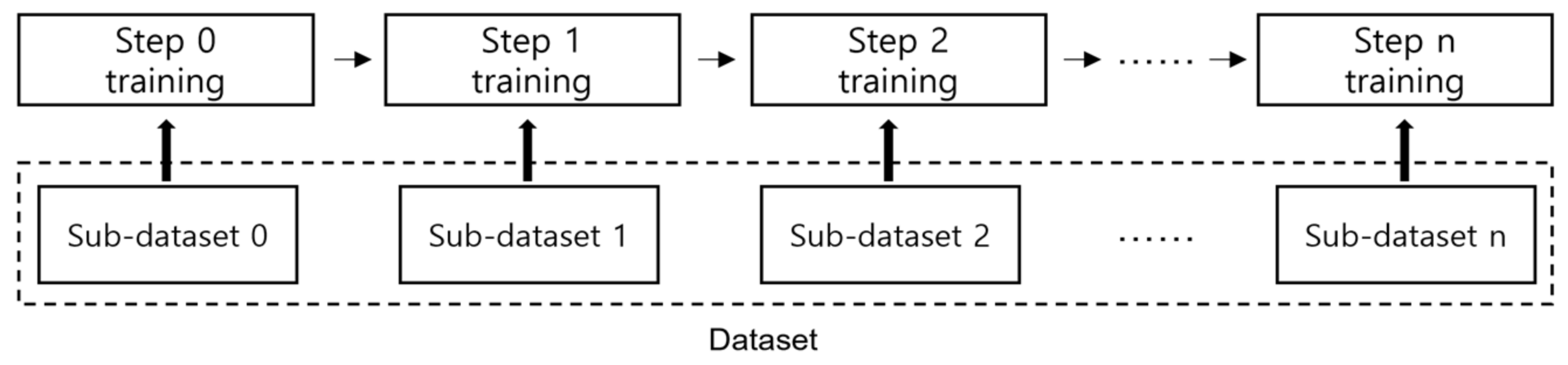
• In our study, old data and old class labels are not reused in the learning process of the s-model. The dataset is used separately in learning as shown in Figure 1. In this process, when the existing loss function of the CenterNet model is used as it is, information on the existing class cannot be learned in the new class learning process. It means there is a problem in that the weight associated with the existing class is changed. We suggest that the loss function associated with the existing class is modified among the loss functions.
• The s-model first learns new classes at the GT and then learns information from the previous class and new class information together at the GT’ to reduce the occurrence of catastrophic forgetting about existing classes when learning new classes.

The rest of this paper is organized as follows. Section 2 examines existing studies on CL and object detection. Section 3 deals with the database scenario and proposes a CL model by applying KD to the anchor-free model and distilling the predictions of the t-model. Section 4 describes how the experimental environment and comparison verification targets are organized to perform the experiment and compare the results. Finally, Section 5 presents the conclusions of the present study and directions for future research.

2. Related Work

2.1. Continual Learning and Knowledge Distillation

In the process of accepting new knowledge, the re-learning of a pre-trained model forgets a large portion of the existing knowledge, and it is difficult to accept new knowledge if the existing knowledge is excessively fixed. This problem is called the stability–plasticity dilemma. Furthermore, the above-described problem of forgetting substantial amounts of existing knowledge is called catastrophic forgetting. The objective of CL is to minimize catastrophic forgetting and determine ideal decision boundaries in continual learning [1,2,4,9,10,11,12].

The part covered in this study is learning without forgetting (LwF) in the green part, and this algorithm is a type that uses the KD method among the various CL fields. The KD-based CL method, a data normalization method, began with the model compression technique proposed by Hinton et al. [5], and its application was extended to CL. The first study to use this method for CL was LwF [2,6].

The application of CL using LwF as an example is a proposed case for classification problems, and most CL studies are still focused on them. However, research subjects are gradually expanding into object detection and semantic segmentation.

As one of the object detection cases to which KD was applied, Shmelkov et al. [13] proposed a KD-based CL model using Fast R-CNN, an object detection model. This study involved class IL, and the LwF technique described above was applied so that the model learning the next time received the information learned previously. In addition, Zhou et al. [14] also proposed a continual learning model with Fast R-CNN with KD, which applied RoI and RPN between the t-model and s-model. The data scenario in both studies were used as a sequence style, and the use of the data in continual learning is described in detail in Section 2.2 [15].

Peng et al. [8] proposed an object detection model that applies distillation techniques to CenterNet and full convolutional one-stage object detection (FCOS) [16], which are object detection models without anchor boxes. This paper has proposed, for the first time, a CL model in an anchor-free model, and the data scenario is disjoint. KD was performed for the output layer rather than the regression type in the two anchor-free models, and inter-relation, a method of distilling the relationship between images, has also been proposed. For the inter-relation, the feature map from the uppermost layer of the decoder was used as the distillation layer. After one batch training, the weight of the heatmap output physically returns to its original state (i.e., the t-model state) by restoring to the next model, among the final output loads of the existing learned model, the output layer related to the previous class. In other words, the purpose is to restore information that has been forgotten in the previous learning process.

Feng et al. [17] used the KD method in GFLV2 [18], a one-stage model, to generate a CL object detection model. Scenarios for the study have been mentioned, but it is not known specifically what style of data utilization methods were used.

Michieli and Zanutti [15] proposed several methods of CL models in the semantic segmentation model DeepLabv3+ [19], utilized distillation techniques, and verified various data scenarios [15,20,21]. Ref. [15] presented good results compared to previous studies by adding three loss functions in addition to the distillation method. That is, to minimize the occurrence of catastrophic aggregation in the CL process, both of the predictions between the t-model and the s-model were distilled using the KD technique. This study also confirmed that KD alone was not sufficiently effective and therefore suggested the following: (1) prototype matching that reduces the movement of feature values, (2) contrastive losses that cause features within the same class to pull each other and cause different features to push each other, and (3) feature sparsity, which reduces the density of existing features in the learning process so that new feature distributions can be constructed.

2.2. Data Scenario

In CL, various scenarios are defined in advance, and the difference in the presence or absence of tasks lies in the scenarios involved. As this study targets a gradual increase in classes without task IDs, this section examines the scenarios of data that can be considered when classes gradually increase.

Data and labels are one-to-one in classification tasks but not in object detection tasks. In the latter, it can be said to be a one-to-many relationship because several labels may exist in one datapoint. In CL research for object detection, if data according to classes are used without considering these matters, then there will be a reused image, which affects accuracy. Therefore, it is necessary to consider whether to exclude data reuse or use data as they are. The problem of labeling should also be considered. Depending on the scenario, it is necessary to define whether to accumulate classes sequentially or label classes corresponding to each turn [15].

In the work by Michieli and Zanutti [15], the following three-case classification was proposed based on several prior studies: sequential, disjoint, and overlapped; the details are as follows.

• Sequential: The image used in the previous learning is not used in the subsequent learning. When there is label information about the previous (old) class in the image used in the subsequent learning, then the information is included in the learning process [15].
• Disjoint: The images used in the previous learning are not used in the subsequent learning. However, in disjoint, if there is label information for the previous (old) class in the new images, then the information is not included in the subsequent learning [15].
• Overlapped: Unlike sequential and disjoint, the images used in the previous learning are also used in the subsequent learning. However, the class label only uses information that has been newly added to the corresponding order of learning [15].

3. Methodology

3.1. CenterNet

In this study, CL is made possible for CenterNet using ResNet-50 as a backbone. This section details the structure, related formulas, and definitions of CenterNet described by Zhou et al. [7].

Figure 2 shows the structure of CenterNet, which includes an encoder structure that is reduced to 16 × 16 × 2048 through a ResNet-50 backbone by inputting 512 × 512 × 3 images, and a decoder structure that uses de-convolution to upscale it to 128 × 128 × 32. After the number of channels is increased to 64 without converting the size from the last layer of the decoder, the output layer is composed of a heatmap, a size map, and an offset map.

The heatmap predicts the location and class classification of an object, and the size map predicts the width and height of the object. When an image is entered into CenterNet, the size is 512 × 512 × 3, but it is 1/4 times (i.e., 128 × 128) that in the output layer; therefore, the offset map predicts a decimal error value to regain its original value when restoring the size.

Furthermore, the entire model structure is a fully convolutional network, excluding the max pooling used in the ResNet backbone. In the study of CenterNet [7], the backbone was changed to various models to detect objects as well as three-dimensional objects or human poses [7]. The final loss function of CenterNet is expressed by Equation (1). Because CenterNet has three final outputs, it has a total of three terms by separately calculating the loss function for each output [7].

$$L_{det} = L_k + {\lambda }_{size}{L}_{size} + {\lambda }_{off}{L}_{off}$$

(1)

For the heatmap $\widehat{Y}$, a focal loss is used, which solves the class imbalance problem between the background and key point in the $L_k$ value of Equation (2).

$$\begin{array}{l}{L}_k= -\frac{1}{N} {\displaystyle {\displaystyle \sum }_{xyc}}\left\{\begin{array}{c}{\left(1 - {\widehat{Y}}_{xyc}\right)}^{\alpha }\log \left( {\widehat{Y}}_{xyc}\right) if Y_{xyc} = 1\\ \begin{array}{c}{\left(1 - Y_{xyc}\right)}^{\beta }{\left({\widehat{Y}}_{xyc}\right)}^{\alpha }\\ \log \left(1 - {\widehat{Y}}_{xyc}\right)\end{array} otherwise\end{array}\right.\\ L_{off} = \frac{1}{N}{\displaystyle {\displaystyle \sum }_p}\left|{\widehat{O}}_{\tilde{p}} - \left(\frac{p}{R} - \tilde{p}\right)\right|\\ L_{size} = \frac{1}{N}{\displaystyle {\displaystyle \sum }_{k=1}^N}\left|{\widehat{S}}_{p_k} - S_k\right|\end{array}$$

(2)

In the experiment, $\alpha$ = 2, $\beta$ = 4, $N$ is the number of key points in the image, and $I$ is the value for normalization [7]. The offset $\widehat{O}$ is calculated using the second line $L_{off}$ of Equation (2), and the predicted object size $\widehat{S}$ is equal to the last line $L_{size}$ of Equation (2). The offset and object size are calculated using the $L_1$ loss function [7].

3.2. Prediction Distillation of Teacher Model

This section describes the method used to distill the prediction of the t-model proposed in this study in detail. The anchor-free model targeting the object detection model consists of a final output layer as a matrix. In other words, if the KD technique commonly used in object detection is applied to the anchor-free model as it is, then it is learned by minimizing the differences between the specific layers of the t-model and the s-model. Similar studies have previously noted that it is difficult to expect a significant effect using this method. Unlike the anchor model, which only operates with the results calculated in the KD process (for example, heatmap channels contain not only object-centered information but also noise information around them), unnecessary information in the KD process must be calculated in an anchor-free model.

The method proposed in this study allows the s-model to use the results predicted by the t-model as ground truth (GT). In other words, the top three layers of t-model prediction—which are a heat map, a size map for the width and height of an object, and an offset map for object-centered position correction—are used to make it the same form as GT. The result of the t-model is referred to as ‘t-pred’, and when it is combined with GT, it generates another GT called GT’. In other words, the t-model newly labels images to learn, and the t-model teaches the s-model to view the image from the perspective of the t-model. This method enriches the label information, thereby increasing the knowledge that the s-model needs to learn.

Because the heatmap information predicted by the t-model is output through an activation map and has a narrower range of key points than the heatmap information used by GT, the previously extracted object location and information are used to generate the new heatmap with a Gaussian filter.

When the width of the input image is W and the height is H, stride R is applied to the output image, such that the width and height are W/R and H/R, respectively. We define C as the number of classes. As shown in Figure 2, the component of GT, which is a measured value, is called GT and consists of five values in total.

The heatmap is defined as $H{M}^{GT} \in {\left[0,1\right]}^{W/R\times \mathrm{H}/\mathrm{R}\times C}$, and $W{H}^{GT} \in {ℝ}^{50\times 2}$ refers to the width and height of the objects. $Ob{j}^{GT} \in {\left[0,1\right]}^{50}$ determines the presence or absence of an object and determines whether to use a value of other matrices. $Cente{r}^{GT} \in {ℝ}^{50}$ is obtained by changing the value of the 2D key point to 1D. Since the output image is $1/R$ times, it consists of an $Offse{t}^{GT} \in {ℝ}^{50\times 2}$ value for correcting the center value. The constant value of 50 is an arbitrary definition of the number of objects, and it can be changed.

In CL, class $C$ is $C = C^{°} \cup C^n$. According to the scenario, $C^{°}$ is the existing learned old class, and $C^{°} = \left\{C_1^{°}, \dots , c_n^{°}\right\}$; $C^n$ is a new class to be newly learned, and $C^n = \left\{c_1^n,\dots ,c_m^n\right\}$. That is, the number of detectable classes after the entire scenario is completed is expressed as $n + m$. The number of heatmaps $C^{°+n}$ for GT in Figure 2 represents both $C^{°}$ and $C^n$.

To use t-pred for new learning, when the result of the prediction score ${\widehat{Y}}_{x_i{y}_{i}c}^t$ of the t-model’s predicted object is ${\widehat{Y}}_{x_i{y}_{i}c}^t > th$, it is made to be in the same form as GT. Combining this with GT, $C^{°}$ and $C^n$ are learned simultaneously in the learning process. The newly created t-model prediction and GT are referred to as the GT’. This is created through the combination of t-pred and GT. $H{M}^{GT}$, which is a newly generated heatmap, changes $H{M}_c^{GT}$ of channel $c$ corresponding to $H{M}_c^t > 0$ to $H{M}_c^t.$ Furthermore, as shown in Figure 2, the other four components are combined in the two matrices.

There are a couple of problems associated with the proposed method. The first problem is that the predictions proposed by the t-model are not all correct. The second problem is that objects subject to new labels are predicted to be different objects in the t-model.

The first problem, the proposal of the t-model, can be solved using it as predictive information for the t-model only when the score of what is recognized as an object is greater than or equal to a certain score, that is, ${\widehat{Y}}_{x_i{y}_{i}c}^t > th$. The second problem, when an object to a new label is predicted to be another object in the t-model, can be solved through an IoU comparison of both t-pred and individual objects in GT and not using the prediction of the t-model if the IoU exceeds a certain value, such as a threshold.

3.3. Knowledge Distillation of Output Layers

The proposed method in Section 3.2 cannot be a perfect method with which to distill the previous model knowledge if there seems to be no object in the images that is a previous object. To solve this problem, three final output layers containing all the information in the t-model are directly distilled with the $L_1$ loss function. However, in the case of a heatmap, it is necessary to distill the feature map before applying the sigmoid function because some information disappears during the sigmoid process.

Existing research dealing with the object detection CL model has confirmed that KD was not used well for the size map or for calculating the boundary box of the object [8]. However, if the size of the new object differs from the size of the existing learned object, then the weight information of the size map may vary substantially during the learning process; therefore, KD is applied to all three final output layers in this study.

Since the number of classes in the heatmap of the s-model is greater than that in the t-model’s heatmap, only the channels in the heatmap related to previously learned classes of the s-model are selected to calculate with the t-model’s heatmap. Accordingly, the $L_1$ loss is calculated with ${\widehat{Y}}_s{}^{c^{°}}$, which contains only the heatmap for class $C^{°}$ of s-model. The loss function $L_{kdHM}$ between ${\widehat{Y}}_t$ and ${\widehat{Y}}_s{}^{c^{°}}$ can be confirmed by Equation (3). The loss is calculated using the elements of the matrix to obtain the average. In this equation, the height $H/R$ of the downsampled output layer is defined as $H^{\prime }$, and $W/R$ is defined as $w^{\prime }$. $C$ denotes the number of channels (i.e., the number of classes), wherein the number is the number of classes used in subsequent learning.

$L_{kdWH}$ is the same as the second line of Equation (3), and $L_{kdOff}$ is the same as the third line of Equation (3). The two loss functions perform element-specific calculations on the two channels because the t-model and s-model have the same hierarchical structure. This loss function also uses the $L_1$ loss function.

$$\begin{array}{l}{L}_{kdHM} = {\displaystyle {\displaystyle \sum }_{W^{\prime }{H}^{\prime }{C}^{°}}}\left|{\widehat{Y}}_t-{\widehat{Y}}_s{}^{c^{°}}\right| \\ L_{kdWH} = \sum \left|{\widehat{S}}_t - {\widehat{S}}_s\right|\\ L_{kdOff} = \sum \left|{\widehat{O}}_t - {\widehat{O}}_s\right|\end{array}$$

(3)

3.4. Total Loss Function of the Proposed Model

In this study, because the GT and predicted values of the t-model are combined through the proposed GT’, the loss function of the s-model is calculated with the GT included in the GT’. In CL, the original loss function of the learning model is typically calculated before calculating the loss function for CL. However, in this study, the original loss function is changed without being used as it is. This can be attributed to the relationship between the disjoint data scenario and the GT.

When using a disjoint data scenario, the GT has no label information related to the old class $C^{°}$. For example, in the 19 + 1 scenario, during the process of s-model learning, the heatmap does not contain any information on channels 0 to 18 (old class), because it only has information on channel 19 (new class). When the loss is calculated using this heatmap, the deep learning model learns by recognizing that there are no objects from 0 to 18 in this process. Therefore, if the existing loss function is used as it is, there is a possibility wherein the recognition accuracy for old classes label may decrease during the learning process due to confusion in the contents of channels 0 to 18.

Unlike other previous studies that leave the original loss function intact, our study proposes a modification to the heatmap used for the existing loss function. The losses between the GT and predicted heatmaps are subjected to the process of minimizing focal losses for all channels corresponding to the entire class; however, channels corresponding to the previous label are cut off. As a result, the catastrophic forgetting that occurs during the learning process can be removed. The changed equation is the same as that in Equation (4), and $c^n$ represents a new class.

$$L_k^{c^n}= - \frac{1}{N} {\displaystyle {\displaystyle \sum }_{xy{c}^n}}\left\{\begin{array}{c}{\left(1 - {\widehat{Y}}_{xy{c}^n}\right)}^{\alpha }\log \left( {\widehat{Y}}_{xy{c}^n}\right) if Y_{xy{c}^n} = 1\\ \begin{array}{c}{\left(1 - Y_{xy{c}^n}\right)}^{\beta }{\left({\widehat{Y}}_{xy{c}^n}\right)}^{\alpha }\\ \log \left(1 - {\widehat{Y}}_{xy{c}^n}\right)\end{array} otherwise\end{array}\right.$$

(4)

When the loss function in CenterNet considers the local loss for the heatmap as $L_k$ as defined above, the size map $L_1$ loss is $L_{size}$, and the offset map is $L_{off}$. The loss function $L_{det}$ of the existing CenterNet is the same as Equation (1) defined above. The modified heatmap operation is referred to as $L_k^{c^n}$ in Equation (4), and the applied formula is defined in Equation (5) by $L_{oridet}$.

$$L_{oridet} = L_k^{c^n} + {\lambda }_{size}{L}_{size} + {\lambda }_{off}{L}_{off}$$

(5)

In this case, the loss function of GT’ is defined by Equation (6) $L_{newdet}$, and it follows the existing loss function for the entire class channel; the weight is also the same. $L_k^{\prime }$, $L_{size}^{\prime }$, and $L_{off}^{\prime }$ are the same as previously defined $L_k$, $L_{size}$, and $L_{off}$, but the loss calculation target is changed from the existing GT to GT’. The final loss function is given in Equation (7). ${\lambda }_{newdet}$ is used as a factor to suppress excessive distillation and increase new learning.

$$L_{newdet} = L_k^{\prime } + {\lambda }_{size}^{\prime }{L}_{size}^{\prime } + {\lambda }_{off}^{\prime }{L}_{off}^{\prime }$$

(6)

$$\begin{array}{cc}{L}_{tot}\hfill & = L_{oridet} + {\lambda }_{newdet}{L}_{newdet}\hfill \\ & + {\lambda }_{kdHM}{L}_{kdHM} + {\lambda }_{kdWH}{L}_{kdWH} + {\lambda }_{kdoff}{L}_{kdoff}\hfill \end{array}$$

(7)

4. Experiment

4.1. Experiment Environment

The learning environment used for training and testing in this study was a workstation with an Intel (R) Core (TM) i9-10900F CPU @ 2.80 GHz, 64 GB RAM, a GeForce RTX 3090 GPU, and the deep learning framework consisting of Python 3.6, Anaconda 3, and Pytorch 1.7.1. The code of CenterNet used was the official code [22] posted by the author of this paper. In the experiment in the present work, like the existing CenterNet experiments, 70 epochs of learning were performed in total, and the learning rate changed over a total of two times. The existing learning rate was 1.25 × 10⁻⁴, and the change point was reduced by one-tenth in each of the 45th and 60th epochs. To control some of the randomness, functions related to reproducibility [23] covering the Pytorch official site were referred to and used.

After learning the t-model in advance, the class of the s-model increased the number of heatmaps by the new class through the scenario. The weight of the pre-trained t-model was brought to the s-model when initialized before learning. In this process, the weight-loading function provided by the deep learning framework, such as Pytorch, was used. However, a weight was not called when the name of the layer or the number of channels was different. If this problem is not solved, then the previously learned information will be lost even before learning; therefore, the heatmap of the s-model will be sliced by the number of previous learning classes to force weight loading. For bias, only initialization was performed. The same dataset and scenario were used for each comparative experiment, and the database used a disjoint data structure.

4.2. Comparison Verification Configuration

Most CL studies simultaneously use several approaches in combination with algorithms. It is difficult to find a clear comparative verification target in the CL model for object detection. Therefore, a comparative verification method of applying the algorithm proposed in the previous study to certain models, such as object detection, is generally used; the model in our study is CenterNet. Regardless of the performance of the model itself, we confirmed that our approach minimizes catastrophic forgetting and increases the accuracy of the new learning.

In this study, sparse and differentiated latent representations (SDR) proposed by Michieli and Zanuttigh [15], LwF [6], and SID [8] were selected for comparison. Because there are the wide variety of CL approaches and there are not many comparison targets that can meet the limitations of this study, existing studies that use the KD technique and do not store samples were selected as comparison targets. When the backbone or detection model was different, it was changed and compared appropriately with CenterNet.

In the CenterNet official code of [22], the structure of the up-convolution process and the process of generating the final output layer, such as convolution, batch normalization, and application of activation functions, were constructed in a sequential class provided by Pytorch. In this case, the feature map output from the internal layer grouped by sequential class could not be used directly from the loss function.

In our study, the selective and inter-related distillation (SID) method proposed by Peng et al. [8] was used as a comparison target. In the CenterNet official code, several of the distillation layers had been utilized inside the structure using the sequential class function of Pytorch. Accordingly, the sequential class function created for the final output layer was maintained as it was, but the weight value by input could be separately generated for each layer in our study to compare with our approach. The feature map output obtained using this process could be used as the loss function. Some values may have changed in response to structural changes.

As a comparison index of accuracy, the present work used the most used mean average detection (mAP) in the object detection model, and as an additional comparison index, it also used the $F{1}^i$ score of the harmonization mean recognition (8) for CL proposed by Peng et al. [8], where i means incremental, $P_{old}$ is the mAP of the label related to previous learning, and $P_{new}$ is the mAP of the newly added label [8].

$$F{1}^i = 2 \times \frac{P_{old} \times P_{new}}{P_{old} + P_{new}}$$

(8)

4.3. Experimental Results

In the case of the PascalVOC 2007 and 2012 data used for learning, ‘trainval’, a material provided from the official site, was downloaded, and the ‘trainval.txt’ data contained in the downloaded folder was used for training, whereas the PascalVOC 2007 test data was used for testing. To create a CL scenario, a set of usage data for each scenario was defined based on the text data for each class located in the Main folder inside the ImageSets folder. First, the text data corresponding to the first learning class was read in alphabetical order and combined into one, except for overlapping image names, to be used as the first learning data. If there was an object corresponding to the second learning class inside the image, then its label was not used. The data for the second learning scenario read and used the remaining text data file, excluding the overlapping image names. In this process, two conditions needed to be satisfied: first, the image could not be used for primary learning; second, even if it was a new image, the label could not be used if the class corresponding to primary learning existed in the image.

We proposed anchor-free CL as part of a knowledge distillation modification scheme in a limited environment that does not reuse data and avoids increasing parameters or layers. We used the t-model as a tool for labeling; its result, t-pred, was combined with the GT of the new learning process. Since GT only has new labels, it causes catastrophic forgetting of existing labels. However, when combined with t-pred, information from existing labels is added, thus allowing it to play a role in learning, such as general learning.

The backbone used in CenterNet for our proposed model was ResNet-50. During the experiment, among the options provided by the official code of CenterNet, ‘nms’ and ‘flip_test’ were used. All the experiments in this section used the same option as the verification data: ${\lambda }_{size}$ = 0.1, ${\lambda }_{off}$ = 1, ${\lambda }_{size}^{\prime }$ = 0.1, ${\lambda }_{off}^{\prime }$ = 1, ${\lambda }_{newdet}$ = 1, and ${\lambda }_{kdHM}$, ${\lambda }_{kdWH}$, and ${\lambda }_{kdoff}$ are 0.3. The result was the mean average decision (mAP), which was rounded to the third decimal place. In the proposed method, the t-model prediction value of the t-model predictive distillation was fixed at 0.2, and the IoU was fixed at 0.8; these were fixed at the same values in all experiments below.

For CenterNet used in this study, ResNet-50, which has relatively low complexity and low accuracy, was used as a backbone to compare the algorithm results for the CL approach; therefore, we could expect to achieve an increase in basic accuracy by changing the backbone model or applying another type of anchor-free model.

Table 1. Comparison of 19 + 1 Scenario (%).

Class	20 Classes	19 Classes	Fine Tuning	LwF [6]	SID [8] $\mathit{k} = 2$	SID [8] k = 3	SID [8] k = 4	SDR [15] KD1	SDR [15] KD2	Proposed
aeroplane	73.7	76.6	10.7	41.9	62.5	59.5	52.4	67.7	54.1	69.1
bicycle	79.1	81.2	11.7	33.5	66.7	68.3	62	73.7	63.5	78.2
bird	70.6	72.1	26.1	34	52.1	41.1	25.9	64.5	58.1	64.6
boat	62.6	60.1	11.7	26.1	36.7	27.9	14.9	49.7	35.4	49
bottle	56.9	54.5	8.5	21.5	38.4	24.7	30.4	47.9	28.3	50.1
bus	79.1	77.7	12.9	38.9	64.1	61.8	52.3	66.1	34.7	72.1
car	83.7	84.3	14.4	45.5	64.3	76.2	70.8	48.7	34.1	73.6
cat	81.2	80.5	49	58.4	68.7	44.8	18.2	78	74.8	76.2
chair	58.4	58.6	9.1	21.4	35.4	39.6	37.1	40.5	24.4	49.8
cow	78.8	79.5	30.4	60.6	69	67.1	54.9	73.3	66.9	74.6
diningtable	70.5	67.5	11.6	22.3	58.1	56.7	57.6	59.1	54	65.7
dog	79.3	78.5	27.3	39.5	66.8	57.8	41.7	72.1	65.8	71.9
horse	81.6	84	14.4	40.9	67.2	61.7	42.8	78.1	62.9	78.4
motorbike	79.3	81.9	0.5	10.9	59.1	73	61.1	65.3	49.4	70.2
person	78.7	79.4	27.5	57.1	65.6	53	38.9	73.7	68.1	77.5
pottedplant	47.7	45.5	9.1	17.8	30.8	23.6	28.5	34.1	29.3	40.6
sheep	77.9	77.6	40.5	45	68.9	60.5	48.9	70.7	69.9	77.1
sofa	70.1	69.7	19.5	33.1	58.5	40.5	24.3	58.4	51.5	63.4
train	79.1	79.5	27.2	54.3	63.5	63.9	57.6	71.7	54.4	73.7
tv/monitor	73.4	-	42.4	22.6	16.4	15.9	12.5	13.9	17.2	27.7
mAP	73.1	73.1	20.2	36.3	55.6	50.9	41.6	60.4	49.8	65.2
1–19 mAP	-	73.1	19	37	57.7	52.7	43.2	62.8	51.5	67.1
20 mAP	-	-	42.4	22.6	16.4	15.9	12.5	13.9	17.2	27.7
$F{1}^i$	-	-	26.3	28.1	25.5	24.4	19.3	22.8	25.8	39.2

lists the experimental results of the 19 + 1 scenario. $k$ of SID [10] was the number of samples for the inter-relation proposed by SID [8], and SDR [15] was divided into KD1 for distilling only heatmaps according to the model of CenterNet [7] and KD2 for distilling both heatmaps and the WH output layer. The worst result of mAP was obtained using the fine-tuning method, but the result of secondary learning (related to the ‘tv/monitor’ class) was the best. This is because catastrophic forgetting was not considered at all in the fine-tuning method.

In the case of LwF, $F{1}^i$ showed the best results among the comparison targets; however, when looking at mAPs of 1–19, it appears that there was substantial forgetting of the existing classes. This finding shows that, even with a CL approach that yields good results in the classification model, it is difficult to apply it to the object detection model for the original shape, thus proving the need for a unique method for object detection.

In SID, it depended on the number of samples; however, when looking at the $F{1}^i$ scores, the best result was obtained when using $k =$ 2. Forgetfulness of existing object knowledge was resolved to some extent, but new learning remained in the 16.4% mAP range; therefore, this was judged not to be the best method. SDR was not very effective in CenterNet, although it has shown good performance in semantic segmentation models. The mAP of it showed good results, and the catastrophic forgetting seemed to have been resolved to some extent; however, the $F{1}^i$ and the learning results of the new class were not good, thus making it difficult to use the model in real fields. The proposed model compared to the SID (k = 2), which is the target of comparison, showed good results of 9.6% p based on mAP and 13.7% p based on $F{1}^i$.

Table 2. Comparison of 15 + 5 Scenario (%).

20 Classes	20 Classes	15 Classes	Fine Tuning	LwF [6]	SID [8] $\mathit{k} = 2$	SID [8] $\mathit{k} = 3$	SID [8] $\mathit{k} = 4$	SDR [15] KD1	SDR [15] KD2	Proposed
aeroplane	73.7	74.9	26.4	9.1	59	44.3	33.7	51.9	2.3	68
bicycle	79.1	81.3	0	9.1	77.3	77.5	76.4	75.7	38.4	78.9
bird	70.6	70.1	9.1	9.1	53.8	54.4	54.9	52	14.3	61.7
boat	62.6	60.3	4.9	25.6	51.4	55.6	53	8.5	0	56.2
bottle	56.9	54.7	9.1	0	41.9	48.3	44.3	15.9	0.3	49.7
bus	79.1	76.6	0	6.1	63.9	55.2	70.2	41.4	7.3	54.9
car	83.7	84.1	34.8	16.2	77.6	79.1	79.4	38.8	34.8	79.8
cat	81.2	79.6	9.1	0	62.1	53.7	53.7	73.4	50.4	78.6
chair	58.4	56.9	9.1	0	43.7	48.9	50.9	28.7	13.4	50
cow	78.8	70.5	18.4	0	54.5	36.8	54.4	46.8	14	51
diningtable	70.5	63.1	0	0	60.3	59.3	56.2	54.1	0.3	61.2
dog	79.3	76.1	7.7	0	67.8	61.7	57	56.8	33.3	52.7
horse	81.6	82.9	27.2	0	79	78.6	77.9	73.7	41.5	75.4
motorbike	79.3	81	0	9.1	68.3	75.9	75.7	59.5	23.4	71
person	78.7	79.2	35.2	27	74.8	76.7	77.3	72.8	48.6	77
pottedplant	47.7	-	21.4	18.7	19.2	9.5	0.8	9.8	18.3	15.9
sheep	77.9	-	19.2	19.1	15.5	14.9	14.3	12.6	15.3	15.8
sofa	70.1	-	38	35.5	27.3	19.4	16.1	14.9	29.1	26.7
train	79.1	-	14.5	22.8	12.9	11.2	9	14.7	13.7	21.7
tv/monitor	73.4	-	41.3	32.5	37.1	17.1	12.4	26.4	39.9	34.5
mAP	73.1	72.8	16.3	12	52.4	48.9	48.4	41.4	21.9	54
1–15 mAP	-	72.8	12.7	7.4	62.4	60.4	61	50	21.5	64.4
16–20 mAP	-	-	26.9	25.7	22.4	14.4	10.5	15.7	23.3	22.9
$F{1}^i$	-	-	17.3	11.5	32.9	23.3	17.9	23.9	22.3	33.8

presents comparative experiments with existing studies according to the 15 + 5 scenario. In this result, the worst method of mAP was the method of LwF. The simple LwF method was not suitable for an anchor-free model such as CenterNet. Rather, the mAP was slightly higher in fine tuning, which appears to be due to the addition of five classes, thus resulting in increased detection accuracy for five classes while learning about new classes in the data. In SID, when considering both mAP and $F{1}^i$ scores, the best results were shown when k was 2. Among the newly added classes, the results of ‘train’ were slightly poor. SDR showed lower mAP and $F{1}^i$ scores than SID, and the model proposed in this study also showed the best results in this experiment. Relative to the comparison target SID (k = 2), the proposed model exhibited good results of 1.6% p for mAP and 0.9% p for $F{1}^i$.

Table 3. Comparison of 10 + 10 Scenario (%).

20 Classes	20 Classes	10 Classes	Fine Tuning	LwF [6]	SID [8] $\mathit{k} = 2$	SID [8] $\mathit{k} = 3$	SID [8] $\mathit{k} = 4$	SDR [15] KD1	SDR [15] KD2	Proposed
aeroplane	73.7	73.5	0	0	33	60	59	33.2	0.1	56.2
bicycle	79.1	78.4	0	0	58.1	70.2	68	8.3	0.2	67.8
bird	70.6	68.5	0	0	20.6	56.2	58.5	12.2	2.3	37.2
boat	62.6	62.5	0	0	15.3	44.3	39.1	30.5	4.6	38.8
bottle	56.9	54.5	0	0	6.1	35	33.2	5.7	0	42
bus	79.1	74.7	0	0	56.9	63	63.1	24.4	0.1	30.9
car	83.7	84.9	0	0	69	77.9	76.5	56.3	0.2	75.1
cat	81.2	70.7	0	0	46.5	38.7	61.4	45.9	18.1	34.8
chair	58.4	56.7	0	0	29.2	33	42.5	11.6	0.1	48.6
cow	78.8	57.3	0	0	55.2	31.6	29.8	19.3	27.3	40.8
diningtable	70.5	-	50.1	35.7	38.3	38.6	26.4	32.9	49.6	43.1
dog	79.3	-	47.9	35.8	39.5	42.3	27.4	40.6	46.1	47
horse	81.6	-	68.7	60.5	62.8	61.1	51	63.4	68.8	67.5
motorbike	79.3	-	55	44.7	55.1	44.3	36.9	46.2	53.6	60.9
person	78.7	-	75.1	67.1	72.6	70.3	64.1	66.3	74.4	71.8
pottedplant	47.7	-	41.4	29.3	36.3	33	20.5	26.6	41.9	37.5
sheep	77.9	-	66.5	44.9	58.5	58.5	38.2	59.4	65.9	63.5
sofa	70.1	-	55.4	49.1	46.1	48.2	37.8	48.7	55.6	55.4
train	79.1	-	38	31.2	29.7	40.8	30	28.2	36.5	44.1
tv/monitor	73.4	-	62.2	51.8	61.3	58.5	46.9	49.5	57.8	61.6
mAP	73.1	68.2	28	22.5	44.5	50.3	45.5	35.5	30.1	51.2
1–15 mAP	-	68.2	0	0	39	51	53.1	24.7	5.3	47.2
16–20 mAP	-	-	56	45	50	49.6	37.9	46.2	55	55.2
$F{1}^i$	-	-	0	0	43.8	50.3	44.2	32.2	9.6	50.9

lists the experimental results for the 10 + 10 scenario. Overall, when looking at the comparison targets, the proposed model preserved much of the existing knowledge. Given that the results of past learning subjects suffered fatal losses in fine tuning and LwF, if there are newer learning data and new classes, then it is easier for existing information to be forgotten.

However, in our proposed model, the results of the new learning and existing learning subjects appeared to be almost equal. It can also be seen that the inter-relation method showed good results in the experiment of SID ($k$ = 3), which showed the best results among the comparison targets. However, the proposed model showed better results of 0.9% p in mAP and 0.6% p in $F{1}^i$.

The results for each scenario of the proposed model are shown in Figure 3. In scenario 19 + 1, the old labels (person) and new labels (TV/monitor) were detected well as shown in Figure 3a. In scenarios 15 + 5 and 10 + 10, some catastrophic forgetting occurred so that one of the two dogs could not be found properly, and the detection accuracy of the dog was also low as shown in Figure 3b. The motorbike was detected by mistaking it as a car in scenario 10 + 10 as shown in Figure 3c.

4.4. Consideration

In general, whereas the deep learning model only utilizes those with a t-model prediction value exceeding a certain value, this study distilled the prediction of a low t-model prediction value of 0.2, thus allowing the s-model to learn how the t-model looked at the image, even if the actual answer was not obtained. This could be judged as a certain object because the distillation object had a specific characteristic in the detection part even if it was an incorrect answer.

Figure 4 shows the results of the subsequent learning in the 19 + 1 scenario. That is, in the learning, ‘TV/monitor’ was added as a new learning label, and the learning data consisted of a new image with a ‘TV/monitor’ learning label. Figure 4a shows a heatmap created by the image and the object position of the GT, and Figure 4b shows a visualization of the boundary box according to the object position of the GT.

Figure 4c shows the heatmap predicted by the t-model during the s-model learning process, and Figure 4d is a visualization of the boundary box using the heatmap and object position. In this process, ‘TV/monitor’ was not predicted because it was predicted by the model learned in previous learning. However, information that the s-model needed to predict, such as dog and chair, can be seen. Incorrect answers were also proposed.

Figure 4e shows the result of combining the t-model predicted value of higher than 0.2 in Figure 4c and each heatmap in Figure 4a, i.e., this combination is called GT’. Figure 4f shows the results of the boundary box of Figure 4e. Using this result as the GT would be much more effective than distilling the layer, a commonly used KD technique, for the s-model.

However, if there are too little data for subsequent learning, it can be expected that the effect will decrease. Therefore, our suggestion was expected to be more effective if a large amount of label data in the existing previous learning process was used in learning, which is a sequential data scenario learning style.

Another limitation of the proposed method is when the object with the new label was predicted as another object in the t-model; this problem is shown in Figure 5. For example, in the Pascal VOC 15 + 5 scenario, a problem arose wherein a ‘sheep’ as shown in Figure 5a, which was a new label target, was classified as a ‘dog’ in the t-model as shown in Figure 5b.

As mentioned earlier, information comprising ‘even if the object is not the correct answer, it is predicted like a previous object’ is transmitted from the t-model. Therefore, this problem requires information on the measured values and should first use the measured information. In other words, by comparing the individual predictions of the t-model and individual objects in the actual measurement information, it can visually confirm that the problem can be solved by not using the prediction of the t-model when the IoU exceeds a certain value.

5. Conclusions

In this paper, a study was conducted on CL, which has recently attracted increased interest owing to various problems, including the continuously increasing amounts of data, data storage, and copyright issues. CL is gradually increasing its application area in domains such as object detection and semantic segmentation in classification problems.

In this study, KD was applied to the object detection field, and CenterNet, which does not use an anchor box, was changed to a CL model. In addition, by distilling the predictions of the t-model, we proposed a model that can minimize catastrophic forgetting and guarantee some new learning accuracy if there are sufficient learning data each time the next order gradually increases according to the CL scenario.

Because the general object detection deep learning model uses an anchor box, manual work is required for predefined data, but as the increase in the size of the objects cannot be defined in advance, the anchor-free model was used to solve the problem of the anchor box among various hyperparameters.

We proposed GT’ to apply the idea of knowledge distillation to the anchor-free model for class IL. In our work, we used a disjoint data structure method that prohibits the reuse of data. The proposed model in our work avoids increasing parameters, and it does not store feature maps in previous learning. The t-model in the proposed model can label new training data. We call it t-pred, and it uses the labeling data of the t-model in our next learning. T-pred combines with GT to become GT’, which minimizes confusion in model learning, although only new data are included in the new learning material.

For the method proposed in this study, the loss value of the distillation layer should be specified, and the t-model prediction value and IoU threshold used by the t-model are also important hyperparameters; therefore, they should be adjusted according to the amount of new data added and the validity of the t-model’s prediction in the image. These problems can also be efficiently applied to the real environment through the proposal of models that enable hyperparameter automation.

In fact, although many researchers are interested in CL, there have been limited studies applying CL to this point. One potential reason for this is that there are many areas where CL should be applied, but it is difficult to collect data for application. We have previously studied how deep learning is applied to the PCB field, and we have already collected a great deal of data on this topic. We believe that detecting PCB parts based on the proposed CL model will help cope with the increasing number of PCB parts in the future.

References

1. Chen, Z.; Liu, B. Lifelong Machine Learning. In Synthesis Lectures on Artificial Intelligence and Machine Learning, 2nd ed.; Morgan & Claypool Publishers: San Rafael, CA, USA, 2016; Volume 10, pp. 1–27. [Google Scholar]
2. Masana, M.; Liu, X.; Twardowski, B.; Menta, M.; Bagdanov, A.D.; van de Weijer, J. Class-incremental learning: Survey and performance evaluation on image classification. arXiv 2020, arXiv:2010.15277. [Google Scholar]
3. Van de Ven, G.M.; Tolias, A.S. Three scenarios for continual learning. arXiv 2019, arXiv:1904.07734. [Google Scholar]
4. Mai, Z.; Li, R.; Jeong, J.; Quispe, D.; Kim, H.; Sanner, S. Online Continual Learning in Image Classification: An Empirical Survey. Neurocomputing 2021, 469, 28–51. [Google Scholar] [CrossRef]
5. Hinton, G.; Vinyals, O.; Dean, J. Distilling the Knowledge in a Neural Network Geoffrey. arXiv 2015, arXiv:1503.02531. [Google Scholar]
6. Li, Z.; Hoiem, D. Learning without Forgetting. IEEE Trans. Pattern Anal. Mach. Intell. 2017, 40, 2935–2947. [Google Scholar] [CrossRef] [Green Version]
7. Zhou, X.; Wang, D.; Krähenbühl, P. Objects as points. arXiv 2019, arXiv:1904.07850. [Google Scholar]
8. Peng, C.; Zhao, K.; Maksoud, S.; Li, M.; Lovell, B.C. SID: Incremental learning for anchor-free object detection via Selective and Inter-related Distillation. Comput. Vis. Image Underst. 2021, 210, 103229. [Google Scholar] [CrossRef]
9. Delange, M.; Aljundi, R.; Masana, M.; Parisot, S.; Jia, X.; Leonardis, A.; Slabaugh, G.; Tuytelaars, T. A continual learning survey: Defying forgetting in classification tasks. IEEE Trans. Pattern Anal. Mach. Intell. 2021, 44, 3366–3385. [Google Scholar] [CrossRef] [PubMed]
10. Kirkpatrick, J.; Pascanu, R.; Rabinowitz, N.; Veness, J.; Desjardins, G.; Rusu, A.A.; Milan, K.; Quan, J.; Ramalho, T.; Grabska-Barwinska, A.; et al. Overcoming catastrophic forgetting in neural networks. Proc. Natl. Acad. Sci. USA 2017, 114, 3521–3526. [Google Scholar] [CrossRef] [PubMed] [Green Version]
11. Kim, H.-E.; Kim, S.; Lee, J. Keep and Learn: Continual Learning by Constraining the Latent Space for Knowledge Preservation in Neural Networks. Lect. Notes Comput. Sci. 2018, 11070, 520–528. [Google Scholar]
12. Gang, S.; Chung, D.; Lee, J.J. Knowledge Distillation Based Continual Learning for PCB Part Detection. J. Korea Multimed. Soc. 2021, 24, 868–879. [Google Scholar]
13. Shmelkov, K.; Schmid, C.; Alahari, K. Incremental Learning of Object Detectors without Catastrophic Forgetting. In Proceedings of the IEEE International Conference on Computer Vision, Venice, Italy, 22–29 October 2017; pp. 3420–3429. [Google Scholar] [CrossRef] [Green Version]
14. Zhou, W.; Chang, S.; Sosa, N.; Hamann, H.; Cox, D. Lifelong Object Detection. arXiv 2020, arXiv:2009.01129. [Google Scholar]
15. Michieli, U.; Zanuttigh, P. Continual Semantic Segmentation via Repulsion-Attraction of Sparse and Disentangled Latent Representations. In Proceedings of the IEEE/CVF Conference on Computer Vision and Pattern Recognition, Nashville, TN, USA, 25 June 2021. [Google Scholar]
16. Tian, Z.; Shen, C.; Chen, H.; He, T. FCOS: Fully Convolutional One-Stage Object Detection. In Proceedings of the IEEE International Conference on Computer Vision, Seoul, Korea, 28 October 2019; pp. 9626–9635. [Google Scholar]
17. Feng, T.; Wang, M. Response-based Distillation for Incremental Object Detection. arXiv 2021, arXiv:2110.13471. [Google Scholar]
18. Li, X.; Wang, W.; Hu, X.; Li, J.; Tang, J.; Yang, J. Generalized Focal Loss V2: Learning Reliable Localization Quality Estimation for Dense Object Detection. In Proceedings of the IEEE Computer Society Conference on Computer Vision and Pattern Recognition, Nashville, TN, USA, 25 June 2021; pp. 11627–11636. [Google Scholar] [CrossRef]
19. Chen, L.-C.; Zhu, Y.; Papandreou, G.; Schroff, F.; Adam, H. Encoder-Decoder with Atrous Separable Convolution for Semantic Image Segmentation. Lect. Notes Comput. Sci. 2018, 11211, 833–851. [Google Scholar]
20. Michieli, U.; Zanuttigh, P. Knowledge Distillation for Incremental Learning in Semantic Segmentation. arXiv 2019, arXiv:1911.03462. [Google Scholar] [CrossRef]
21. Michieli, U.; Zanuttigh, P. Incremental Learning Techniques for Semantic Segmentation. In Proceedings of the IEEE/CVF International Conference on Computer Vision, Seoul, Korea, 27–28 October 2019. [Google Scholar]
22. GitHub—Xingyizhou/CenterNet: Object Detection, 3D Detection, and Pose Estimation Using Center Point Detection. Available online: https://github.com/xingyizhou/CenterNet (accessed on 24 October 2021).
23. Reproducibility—PyTorch 1.10.0 Documentation. Available online: https://pytorch.org/docs/stable/notes/randomness.html (accessed on 1 November 2021).
Figure 1. Conceptual diagram of continual learning.
Applsci 12 06419 g001
Figure 2. The proposed t-model predictive distillation method.
Applsci 12 06419 g002
Figure 3. The results of each experiment: (a) results of scenario 19 + 1, (b) results of scenario 15 + 5, (c) results of scenario 10 + 10.
Applsci 12 06419 g003
Figure 4. Example of results according to the input image in the 19 + 1 scenario: (a) Example of synthesis of heatmap and input image of GT; (b) bounding box of object in input image of GT; (c) example of synthesis of t-model prediction heatmap and input image of t-model; (d) prediction of t-model bounding box of object in input image; (e) example of heatmap image synthesis of GT’; (f) visualization of GT’ bounding box.
Applsci 12 06419 g004
Figure 5. The GT’ problems and solutions: (a) Labeling of GT’; (b) the result of IoU > 0.8 labeling.
Applsci 12 06419 g005