Computational Intelligence with Wild Horse Optimization Based Object Recognition and Classification Model for Autonomous Driving Systems

Abstract

Presently, autonomous systems have gained considerable attention in several fields such as transportation, healthcare, autonomous driving, logistics, etc. It is highly needed to ensure the safe operations of the autonomous system before launching it to the general public. Since the design of a completely autonomous system is a challenging process, perception and decision-making act as vital parts. The effective detection of objects on the road under varying scenarios can considerably enhance the safety of autonomous driving. The recently developed computational intelligence (CI) and deep learning models help to effectively design the object detection algorithms for environment perception depending upon the camera system that exists in the autonomous driving systems. With this motivation, this study designed a novel computational intelligence with a wild horse optimization-based object recognition and classification (CIWHO-ORC) model for autonomous driving systems. The proposed CIWHO-ORC technique intends to effectively identify the presence of multiple static and dynamic objects such as vehicles, pedestrians, signboards, etc. Additionally, the CIWHO-ORC technique involves the design of a krill herd (KH) algorithm with a multi-scale Faster RCNN model for the detection of objects. In addition, a wild horse optimizer (WHO) with an online sequential ridge regression (OSRR) model was applied for the classification of recognized objects. The experimental analysis of the CIWHO-ORC technique is validated using benchmark datasets, and the obtained results demonstrate the promising outcome of the CIWHO-ORC technique in terms of several measures.

1. Introduction

Autonomous vehicles (AVs) have laid the basis for a new era of smart mobility-based integration with different kinds of techniques, namely radar, cameras, computer vision, and lidar [1]. AV mitigates the user driving problem by implementing smart operations. They could minimize traffic congestion by handling the traffic flow, which results in environmental preservation and lower power utilization. Additionally, AV assists disabled and elderly persons by offering safe and reliable transport schemes [2]. Because of these considerable advantages, there has been growing attention to AVs in the academic and industrial sectors. However, designing reliable autonomous driving is a tedious process [3]. This is due to the fact that a driverless car is a smart agent, which needs to predict, perceive, plan, execute, and decide decisions in real-time, frequently in complex or uncontrolled surroundings, namely an urban area [4]. The major processes for autonomous driving are the quick and accurate identification of pedestrians, vehicles, traffic signs, traffic lights, and objects near the vehicle to ensure safety while driving. In general, AV employs different sensors, including radar, cameras, and lidar, for detecting objects [4]. The object-detection systems of AVs need to fulfill the subsequent conditions: firstly, a higher recognition performance of road objects is required. Next, a real-time recognition speed is significant for the sensors that are utilized in driving. Although certain developments have been achieved in current object-recognition technology used in self-driving vehicles, there is still a possible risk of collision as a motor car is enclosed by several objects during day-to-day use, involving static objects (signs and traffic lights) and uncontrollable moving objects (pedestrians and vehicles). Thus, it is essential to precisely calculate the significance of moving objects and quickly identify different static objects [5,6].

Computation intelligence (CI) has had a dramatic impact on autonomous decision-making. It is a multidisciplinary study field which involves the coordination of different techniques, namely evolutionary algorithms, neurocomputing, fuzzy systems, machine learning, and artificial intelligence methods [7]. The synergy of this technique makes CI an effective mechanism for engineering applications. It could understand the complicated sensory information and consequently react. Certainly, the use of CI for an autonomous system does not simulate an individual’s expertise in decision-making; however, it generally enters a new dimension of intelligence by means of the cooperative understanding of sensory inputs and language patterns driven by the autonomous application through video, audio, text, and so on. In the late 2010s, deep learning (DL) models were used for feature extraction [8]. A hand-crafted feature is optimum since it expresses and extracts feature values through the intended model-based knowledge of the researcher. The DL method could automate feature extraction and is efficient for image detection [9]. DL has attained remarkable outcomes in overall object-detection competitions and the use of image detection needed for autonomous driving (namely semantic segmentation and object recognition) [10].

Numerous object-detection models are available in the literature, which are limited in several aspects [9,10]. Different DL-based models have been developed that could consider different objects, such as dynamic road environments, background lighting conditions, position, dimension, colour, shape, size, etc. Autonomous vehicles require a high capacity for the real-time object detection of road targets. At the same time, the DL models involve several hyperparameters (learning rate, batch size, momentum, and weight decay), and determining the optimal parameters in such a high dimensional space is not a trivial challenge. To resolve this issue, metaheuristic optimization-based hyperparameter tuning techniques are needed. Therefore, this study focuses on the object detection and classification model by the use of hyperparameter tuned DL models.

This study introduces an efficient computational intelligence with a wild horse optimization-based object recognition and classification (CIWHO-ORC) model for autonomous driving systems. The proposed CIWHO-ORC technique primarily derives a new object detection model using a krill herd (KH) algorithm with a multi-scale Faster RCNN model. Additionally, a wild horse optimizer (WHO) with an online sequential ridge regression (OSRR) model was utilized to categorize the recognized objects effectively. The simulation analysis of the CIWHO-ORC technique was examined against benchmark datasets, and the results were inspected under several evaluation measures.

2. Related Works

This section offers a brief survey of existing object recognition models in autonomous systems. In [11], a one-phase object recognition method based on YOLOv4 enhances the recognition performance and supports real-time processes. The neck approach substitutes the SPP with the RFB framework, enhances the PAN framework of the feature fusion method, includes the attention Convolution Block Attention Module (CBAM) and CA architecture to neck and backbone architecture, and lastly, minimizes the complete network width. The backbone of the approach pairs the stacking time of the latter residual block of CSPDarkNet53. In [12], an improved methodology was introduced for identifying ten varieties of objects according to the framework of YOLOv4. As well, a fine-tuning Part Affinity Fields technique was implemented for estimating the pose of pedestrians. Additionally, the Explainable Artificial Intelligence (XAI) technique was included for explaining and assisting the evaluation leads to the risk calculation stage. Chen et al. [13] projected the multi-task learning (MTL) approach for cooperatively modelling distance prediction and object recognition with the Cartesian product-based multi-task combinational method. Moreover, the authors scientifically proved that the presented approach is optimum when compared to the linear multi-task combinational approach, which is commonly utilized in MTL methods.

Li et al. [14] projected a 3D object recognition technique for autonomous driving by completely employing the semantic and geometry, sparse and dense data in stereo images. This approach, termed Stereo RCNN, expands Fast RCNN for stereo input to concurrently subordinate and distinguish objects from left as well as right images. Adding further branches after the stereo Region Proposal Network (RPN) aids in the the prediction of object dimensions, sparse keypoints, and viewpoints that are combined with 2D left-right boxes to estimate a coarse 3D object bounding box. Dai et al. [15] designed an object recognition method for efficient and reliable object recognition in thermal infrared (TIR) images named TIRNet, which is based on convolution neural networks (CNNs). Kim et al. [16] developed an edge-network-enabled real-time object detection framework (EODF). In EODF, AVs extract the region of interest (RoI) of an image taken while the channel quality is not adequately better to support real-time object recognition. Thereby, real-time object recognition is attained because of the decreased communication latency. Mandal et al. [17] focus on identifying three-dimensional objects with three-dimensional bounding boxes that come in the extent of a camera or AGV LiDAR. The primary goal is to utilize DL methods for training the LiDAR and camera images and estimate the confidence score for all the models. Munir et al. [18] presented a DNN Self-Supervised Thermal Network (SSTN) to learn the feature embedding for maximizing the data among infrared and visible spectrum domains by contrasting learning and then employing the learned feature depictions for thermal object recognition with a multi-scale encoder-decoder converter system.

3. The Proposed Model

In this study, a novel CIWHO-ORC technique has been developed to effectively identify the presence of multiple static and dynamic objects such as vehicles, pedestrians, signboards, etc., for autonomous driving systems. The CIWHO-ORC technique encompasses two major processes, namely multi-scale Faster RCNN-based object detection and OSRR-based classification. Additionally, the KH and WHO algorithms were applied to tune the parameters involved in the multi-scale Faster RCNN and OSRR techniques, respectively.

3.1. Object Recognition Module

At the initial stage, the objects that exist in the frame are recognized by the multi-scale Faster RCNN model. Actually, the noticed object is lower in resolution and lesser in size. The present method (e.g., Faster-RCNN) has an optimum detection accuracy for huge objects and could not efficiently detect small objects from the images [19]. An essential purpose is that the individual methods dependent upon DNN create the image computed with convolutional and down-sampled methods for achieving further abstract and higher-level features. All of the down-sampling causes the images to decrease by half. When the object is the same as the size of objects from the PASCAL VOC, the detail of an object’s feature is attained with this convolutional and down-sampling method. However, when the detection of the object is on a very low scale, the last feature is only left with 1–2 pixels after several down-samplings. Thus, some features do not completely describe the features of objects, and the current detection techniques are not efficiently detecting the lesser target objects.

The deeper convolutional function further abstracts the object feature that signifies the higher-level features of objects. The shallow convolutional layer is only extracting the low-level feature of objects. For obtaining higher-level and abstract object features and ensuring that there are sufficient pixels for describing small objects, it integrates the feature of distinct scales to ensure the local details of the objects. This technique has further robust features. The multi-scale Faster RCNN technique was separated into four parts: a primary part is a feature extracting layer that has five convolutional layers (red part), five ReLU layers (yellow parts), two pooling layers (green parts), and three RoI pooling layers (purple part). It can normalize the results of the 3rd, 4th, and 5th convolutional, correspondingly. Figure 1 illustrates the structure of the RPN.

Afterward, the normalizing outcome is sent to the RPN layer and feature-combining layer to the generation of the proposal region (PR) and extracts the multi-scale feature correspondingly. The second part was the feature-combination layer, which joins the distinct scales features of the third, fourth, and fifth layer, as in the 1D feature vector with connection function. The tertiary part was the RPN layer that mostly understood the generating of PRs. The final layer was utilized for realizing the classifier and bounding box regression of the object, which is in PR, and was collected from softmax as well as the bounding box. Obtaining the combinatorial feature vector requires normalizing the feature vector of the distinct scales. Generally, the deeper the convolutional layer output the lesser the scale feature.

Conversely, the lesser the convolutional layer outcomes the better the scale features. The feature scale of distinct layers is widely distinct. The weight of large-scale features is significantly greater than that of smaller-scale features under the network weight that is tuned when the feature of these various scales was integrated, causing the minimum detection accuracy. To prevent large-scale features from covering small-scale features, the feature tensor, which is the output in the distinct RoI pooling, can be normalized before an individual’s tensor is concatenated. It can be utilized when L2 is normalized. The normalized function that is utilized for processing all of the pooled feature vectors was placed afterwards RoI pooling. After normalization, the scale of feature vectors for the third, fourth, and fifth layers are normalized as a unified scale.

$$\widehat{X}=\frac{X}{\Vert X{\Vert }_2},$$

(1)

$$\Vert X{\Vert }_2={({\displaystyle \sum }_{i=1}^d|x_i|)}^{1/2},$$

(2)

where X implies the novel vector from third, fourth, and fifth layer, $\widehat{X}$ has normalizing feature vectors, and $D$ signifies the channel number of all RoI pooling.

$$Y=\gamma \widehat{X},$$

(3)

where $Y={[y_1, y_2, \dots ,y_d]}^T$. During the procedure of error BP, it requires more adjustment to the scale factor $\gamma$ and input vector X. The detailed explanation is as follows:

$$\frac{\partial l}{\partial \widehat{X}}=\gamma \frac{\partial l}{\partial y},$$

(4)

$$\frac{\partial l}{\partial X}=\frac{\partial l}{\partial \widehat{X}}\left(\frac{I}{\Vert X{\Vert }_2}-\frac{X{X}^T}{\Vert X{\Vert }_2^3}\right)$$

(5)

$$\frac{\partial l}{\partial \gamma }={\displaystyle \sum }_y\frac{\partial l}{\partial y}\widehat{X}.$$

(6)

For optimally modifying the hyperparameters of the multi-scale Faster RCNN model, the KH algorithm can be employed. By idealizing the swarm performance of krill, the KH algorithm is a metaheuristic optimization method that solves optimized problems. In KH, the location is affected primarily by the following actions:

• Motion affected by other krills;
• Foraging action;
• Physical diffusion.

In KH, the Lagrangian model [20] was utilized within predetermined searching space as follows

$$\frac{d{X}_i}{dr}=N_i+F_i+D_i$$

(7)

where $N_i$ represent the movement generated by other krill; $F_i$ denotes the foraging movement, and $D_i$ shows the random diffusion of i-th krill. Initially, its direction, ${\alpha }_i$, is decided by the subsequent part: a repulsive effect, target effect, and local effect. Generally, it is described in the following equation

$$N_i^{new}=N^{\max }{\alpha }_i+{\omega }_n{N}_i^{old}$$

(8)

and $N^{\max },$ ${\omega }_n$ and $N_i^{old}$ denotes the maximal speed, the inertia weight, the previous motion, respectively. Next, it is accurately estimated by two mechanisms: the previous experience and food location. For the i-th krill, it is idealized as follows:

$$F_i=V_f{\beta }_i+{\omega }_f{F}_i^{old}$$

(9)

where

$$b_i=b_i^{food}+b_i^{best}$$

(10)

and $V_f$ denotes the foraging speed, ${\omega }_f$ indicates the inertia weight, $F_i^{old}$ represents the last one. The last part is basically a random procedure. It can be estimated according to the maximal diffusion speed and an arbitrary directional vector:

$$D_i=D^{\max }\delta$$

(11)

in which $D^{\max }$ denotes the maximal diffusion speed, and $\delta$ indicates the arbitrary directional vector and array is arbitrary number. Here, the location in KH from $r$ to $r+\mathsf{\Delta }r$ is expressed by:

$$X_i\left(t+Dt\right)=X_i\left(t\right)+Dt\frac{d{X}_i}{dr}$$

(12)

3.2. Object Classification Module

Next to the object detection process, the OSSR technique is utilized for classifying the objects into multiple classes. The OSRR is a faster batch learning model and offers optimal generalization efficiency [21]. OSRR could learn the training data chunk-by-chunk or one-by-one. As OSRR employs a batch learning model, it is utilized to classify microarray data. The online sequential learning in OSRR comprises two phases:

Step 1 Initialization

In this stage, a smaller part of trained data $n_0=\left(x_i,y_i\right),i=1,\dots ,N_0$ with $N_0\in N$ is taken into account to initialize the learning method. The first resultant weight matrix is evaluated based on the RR approah by arbitrarily allocating the input weight $w_j$ and bias $b_j,$ $j=1,2,L$:

$${\beta }^{\left(0\right)}=Q_0{H}_0^T{T}^0$$

(13)

where $Q_0={(H_0^T{H}^0)}^{-1}$ (19) and $H^0$ represent the first hidden state output matrix.

Step 2 sequential learning

Once the new set of observations arrives $n_{k+1}=\left(x_i{y}_i\right)$,

$$Y_{k+1}={\left[y\left({\displaystyle \sum }_{\mathrm{l}=0}^k{N}_1\right)+1,\dots ,y\left({\displaystyle \sum }_{\mathrm{l}=0}^{k+\mathrm{l}}{N}_1\right)\right]}^{\mathrm{T}}$$

(14)

where $\left(k+1\right)th$ denotes the chunk of the data and determines the partially hidden state output matrix $H_{k+1}$ $N_{k+1}$ denotes the number of instances present in the $\left(k+1\right)th$ chunk. Next, by utilizing the output weight upgrade equation as given in the following, the output weight matrix ${\beta }^{\left(k+1\right)}$ could be calculated.

$$Y_{k+1}={\left[y\left({\displaystyle \sum }_{\mathrm{l}=0}^k{N}_{\mathrm{l}}\right)+1,\dots ,\mathrm{y}\left({\displaystyle \sum }_{\mathrm{l}=0}^{k+\mathrm{l}}{N}_{\mathrm{l}}\right)\right]}^T$$

(15)

$$Q_{k+1} ,=Q_K-Q_k,H_{k+1}^T{(1+H_{k+1}Q,H_{k+1}^T)}^{-1}{H}_{k+1}{Q}_k$$

(16)

$${\beta }^{\left(k+1\right)}={\beta }^k+Q_{k+1},{\mathrm{H}}_{k+1}\left(T_{k+1}-H_{k+1}{\beta }^k\right)$$

(17)

Every time a novel chunk of data is attained, the resultant weight matrix was upgraded based on the above equation. The upgraded equation is for one-by-one and chunk-by-chunk learning since the one-by-one data could be taken into account as a special case of the chunk-by-chunk when the chunk size = 1.

To determine the weight and bias values of the OSSR technique, the WHO algorithm was utilized. The WHO approach arithmetically simulates and duplicates the social behavior of wild horses in nature [22]. Horses predominantly live in herds with stallions and several mares and foals. It can display different kinds of behavior, involving commanding, mating, pursuing, grazing, and dominating. Those stages for the WHO approach are shown in the following: Firstly, the population initialization is alienated into various groups. $G$ denotes the amount of groups and $N$ implies the count of the population. Every group has a leader (stallion), hence the count of stallions from the approach equals $G$, and $\left(NG\right)$ indicates the residual population (mares and Foals) are distributed correspondingly amongst this group. 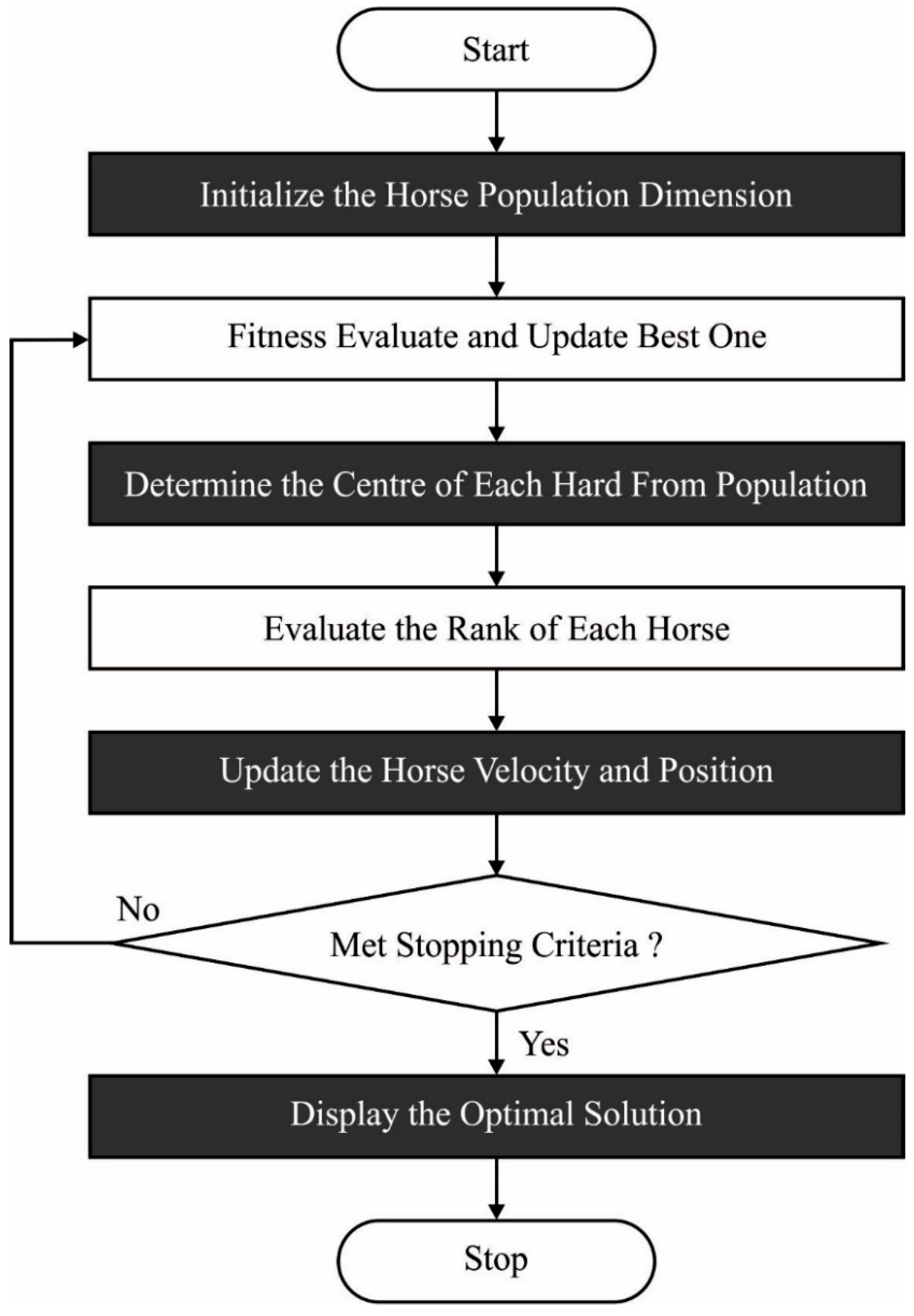Figure 2 depicts the flowchart of the WHO technique.

$$X_{i,G}^j=2Z\cos \left(2\pi RZ\right)\times \left(Stallio{n}^j-X_{i,G}^j\right)+Stallio{n}^j$$

(18)

In which $X_{i,G}^j$ signifies the existing position of the foal or mare group member, $Stallion$ shows the stallion location, $R$ indicate a uniform stochastic value within $\left[-2,2\right]$, and $Z$ indicates the adaptive model estimated as follows:

$$P=\overrightarrow{R_1}<TDR;IDX=\left(P==0\right)$$

(19)

$$Z=R_2\Theta IDX+\overrightarrow{R_3}\Theta \left(\sim IDX\right)$$

(20)

here $P$ indicates a vector consisting of $0$ to $1,$ $\overrightarrow{R_1}$ and $\overrightarrow{R_3}$ represent an arbitrary value within [0, 1], $R_2$ shows a uniform arbitrary value within [0, 1], $TDR$ indicates an adoptive variable that begins with 1 and reduces until it reaches $0$ toward the end of algorithm execution as follows:

$$TDR=1-it\times \left(\frac{1}{maxit}\right)$$

(21)

While it is the existing iteration, $maxit$ indicates the maximal amount of iterations. For implementing the mating behaviors of the horse, a foal goes from group $i$ to a temporary group when a foal goes from group j to a temporary group. For simulating the mating behaviors of horses, the crossover operator of the mean method is presented:

$$X_{G,K}^P=Crossover \left(X_{G,i}^q, X_{G,j}^Z\right)i\ne j\ne k,p=q=end,$$

(22)

$$Crossover=Mean$$

(23)

In the WHO, the Stallion (group leader) led the group to a water hole. The Stallion competes for the water hole, thus the domination group could utilize this water hole initially and other groups could utilize the water hole:

$$\overline{Stallio{n}_{G_i}}=\{\begin{array}{l}2Z\cos \left(2\pi RZ\right)\times \left(WH-Stallio{n}_{G_i}\right)\hfill \\ +WH if R_3>0.5\hfill \\ 2Z\cos \left(2\pi RZ\right)\times \left(WVH-Stallio{n}_{G_i}\right)\hfill \\ -WH if R_3\le 0.5\hfill \end{array}$$

(24)

whereas $\overline{Stalllio{n}_{G_i}}$ represents the following location of the leader. WH shows the place of a water hole. In the subsequent phases, the leader is selected based on fitness value. The leader location and the applicable member would change according to the formula:

$$\overline{Stallio{n}_{G_i}}=\{\begin{array}{l}{X}_{G,i} if \cos t\left(X_{G,i}\right)<\cos t\left(Stallio{n}_{G_i}\right)\hfill \\ Stallio{n}_{G_i} if \cos t\left(X_{G,i}\right)>\cos t\left(Stallio{n}_{G_i}\right)\hfill \end{array}$$

(25)

The WHO algorithm derived a fitness function for optimally tuning the parameters and thereby improved the classifier results. In this work, the classification error rate was considered to be the fitness function, and the WHO algorithm aimed to minimize the classification error rate, as defined in the following:

$$fitness\left(x_i\right)=Classifier Error Rate\left(x_i\right)$$

(26)

$$=\frac{number of misclassified instances}{Total number of instances}\ast 100$$

(27)

4. Results and Discussion

This section investigates the object detection result analysis of the CIWHO-ORC technique on different datasets. The proposed model was simulated using the Python tool. The proposed model was tested using the Python tool. The parameter setting is given as follows: learning rate 0.1, dropout: 0.5, epochs: 50, batch size: 7, activation: ReLU. The proposed model was simulated on the Bdd100k dataset. 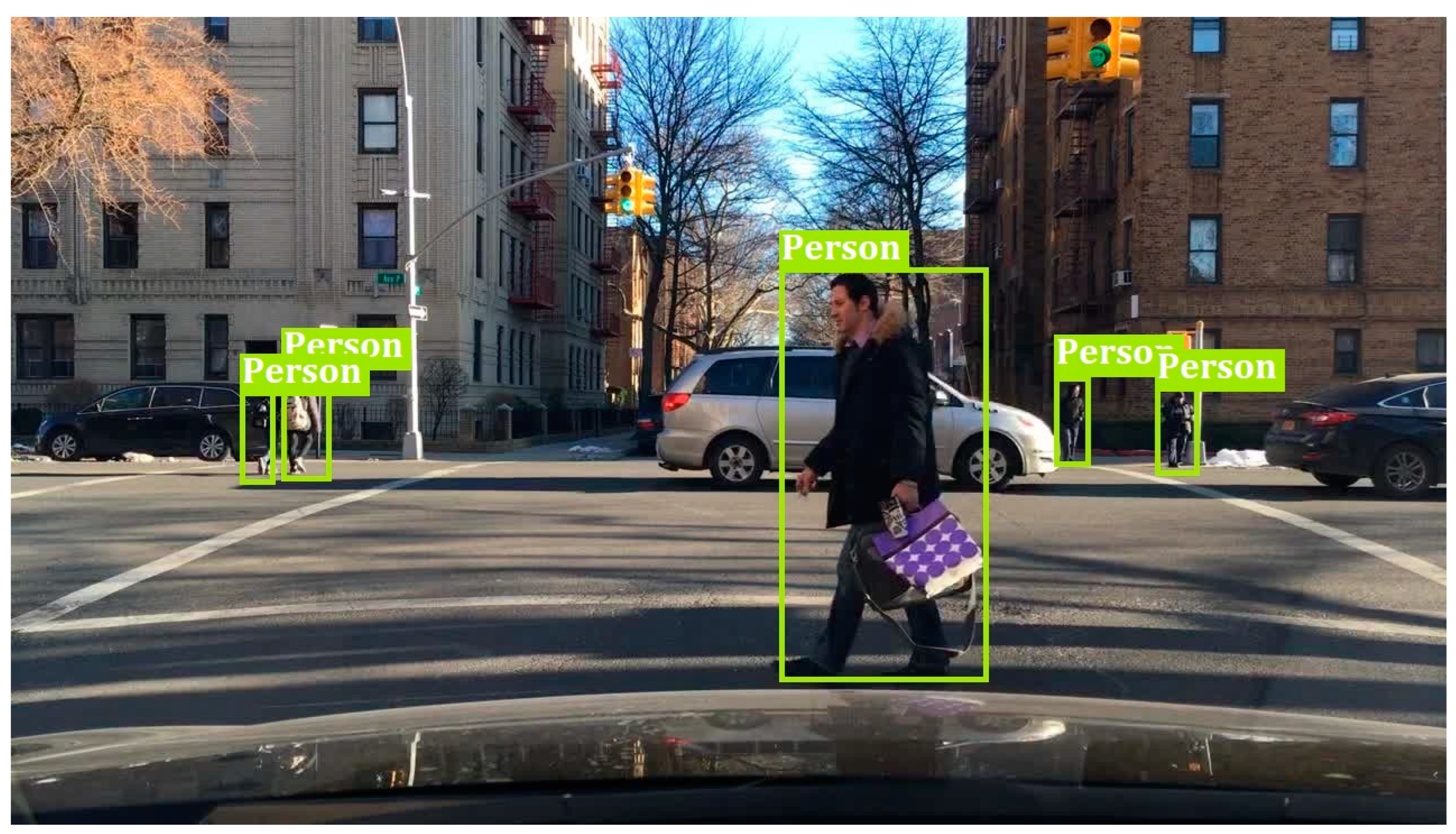Firstly, Figure 3 visualizes a sample of recognized objects in the frame on the test Bdd100k dataset [23]. The figure portrayed that the CIWHO-ORC technique properly identified the objects as ‘persons’ present in the test image.

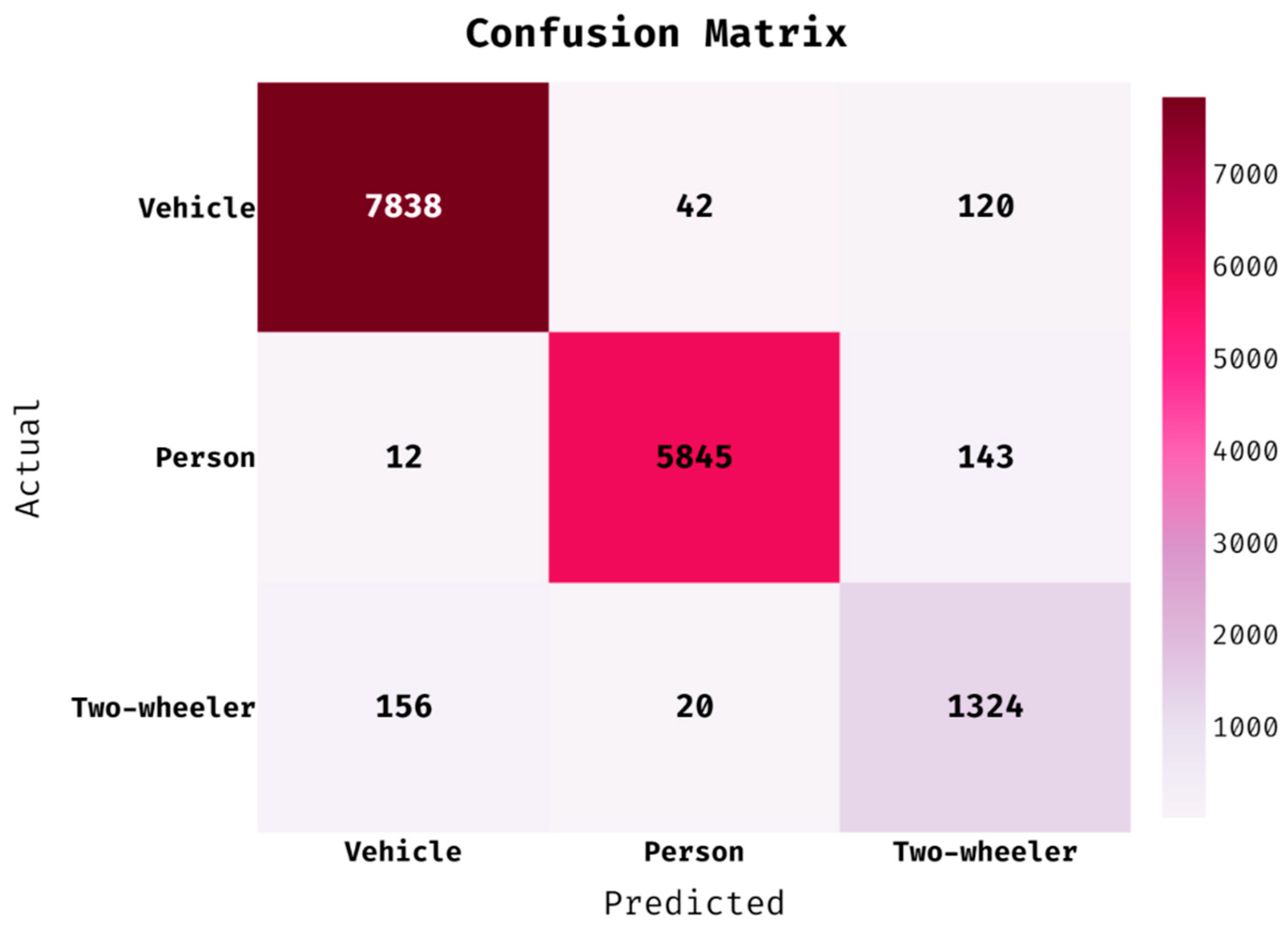
Figure 4 shows the confusion matrix of the CIWHO-ORC technique on the Bdd100k dataset, which comprises three classes such as person, vehicle, and two-wheeler. Figure 4 shows that the CIWHO-ORC technique identified 7838 images under the vehicle class proficiently, 5845 images under the person class, and 1324 images under the two-wheeler class. The values that exist in the confusion matrix are transformed into TP, TN, FP, and FN values in

Table 1. Manipulated values of confusion matrix by CIWHO-ORC technique.

Class Labels	True Positive	False Negative	False Positive	True Negative
Vehicle	7838	162	168	7332
Person	5845	155	62	9438
Two-wheeler	1324	176	263	13,737

.

Table 2. Classification results of CIWHO-ORC technique on Bdd100k Dataset.

Class Labels	Accuracy	TNR	F-Score	MCC
Vehicle	0.9787	0.9776	0.9794	0.9574
Person	0.9860	0.9935	0.9818	0.9705
Two-wheeler	0.9717	0.9812	0.8578	0.8425
Average	0.9788	0.9841	0.9396	0.9235

provides the overall classifier results of the CIWHO-ORC technique under three classes of the Bdd100k dataset. The results exhibit that the Bdd100k dataset has properly identified the three class labels. For instance, the CIWHO-ORC technique identified the ‘vehicles’ with an accuracy of 0.9787, a TNR of 0.9776, an F-score of 0.9794, and an MCC of 0.9574. Similarly, the CIWHO-ORC technique recognized the ‘person’ with an accuracy of 0.9860, a TNR of 0.9935, an F-score of 0.9818, and an MCC of 0.9705. Moreover, the CIWHO-ORC technique recognized the ‘vehicles’ with an accuracy of 0.9717, a TNR of 0.9812, an F-score of 0.8578, and an MCC of 0.8425.

Table 3. APE and ARE Analysis of CIWHO-ORC technique on Bdd100k Dataset.

Methods	Avg. Precision	Avg. Recall	Avg. Prec. −1	Avg. Prec. −2	Avg. Prec. −3
YOLO-v3	0.485	0.817	0.768	0.425	0.261
C-Net Model	0.591	0.847	0.800	0.620	0.354
ASPPC-Net Model	0.612	0.850	0.807	0.632	0.397
CIWHO-ORC	0.691	0.890	0.863	0.715	0.495

provides a brief comparative analysis of the CIWHO-ORC te chnique on the test Bdd100k dataset in terms of the average precision (APE) and average recall (ARE). The results show that the CIWHO-ORC technique enhanced the outcomes of the classification of objects. With respect to APE, the CIWHO-ORC technique obtained a higher APE of 0.691, whereas the YOLO-v3, C-Net, and ASPPC-Net techniques attained a lower APE of 0.485, 0.591, and 0.612, respectively. At the same time, with respect to ARE, the CIWHO-ORC technique reached a maximum ARE of 0.890, whereas the YOLO-v3, C-Net, and ASPPC-Net techniques resulted in a minimal APE of 0.817, 0.847, and 0.850, respectively.

The comparative APE and ARE analysis of the CIWHO-ORC technique on the recognition of small and large objects is shown in

Table 4. APE and ARE Analysis of CIWHO-ORC technique on Small and Large Object Classification.

Methods	Avg. Precision		Avg. Recall
	Small	Large	Small	Large
YOLO-v3	0.481	0.631	0.803	0.912
C-Net Model	0.688	0.675	0.845	0.852
ASPPC-Net Model	0.706	0.665	0.848	0.853
CIWHO-ORC	0.710	0.902	0.882	0.926

. The table values exhibit that the CIWHO-ORC technique offered effective classification outcomes with the maximum values of APE and ARE. For instance, with small-object detection, the CIWHO-ORC technique increased the ARE to 0.710, whereas the YOLO-v3, C-Net, and ASPPC techniques reduced the ARE to 0.481, 0.688, and 0.706, respectively. Simultaneously, with large-object detection, the CIWHO-ORC technique improved the ARE to 0.882, whereas the YOLO-v3, C-Net, and ASPPC techniques reduced the ARE to 0.803, 0.845, and 0.848, respectively.

Another comparison study of the CIWHO-ORC technique on the identification of tiny objects is shown in

Table 5. APE and ARE Analysis of CIWHO-ORC technique on Tiny Object Classification.

Method	Avg. Precision (Tiny)	Avg. Recall (Tiny)
YOLO-v3	0.121	0.614
C-Net Model	0.153	0.802
ASPPC-Net Model	0.154	0.816
CIWHO-ORC	0.185	0.864

in terms of the APE and ARE. The results show that the CIWHO-ORC technique outperformed the other methods with the maximum classification results. Based on the APE of tiny object detection, the CIWHO-ORC technique resulted in an increased APE of 0.185, whereas the YOLO-v3, C-Net, and ASPPC techniques decreased the APE to 0.121, 0.153, and 0.154, respectively. Concurrently, based on the ARE for tiny-object detection, the CIWHO-ORC technique led to an improved ARE of 0.864, whereas the YOLO-v3, C-Net, and ASPPC techniques decreased the APE to 0.614, 0.802, and 0.816, respectively.

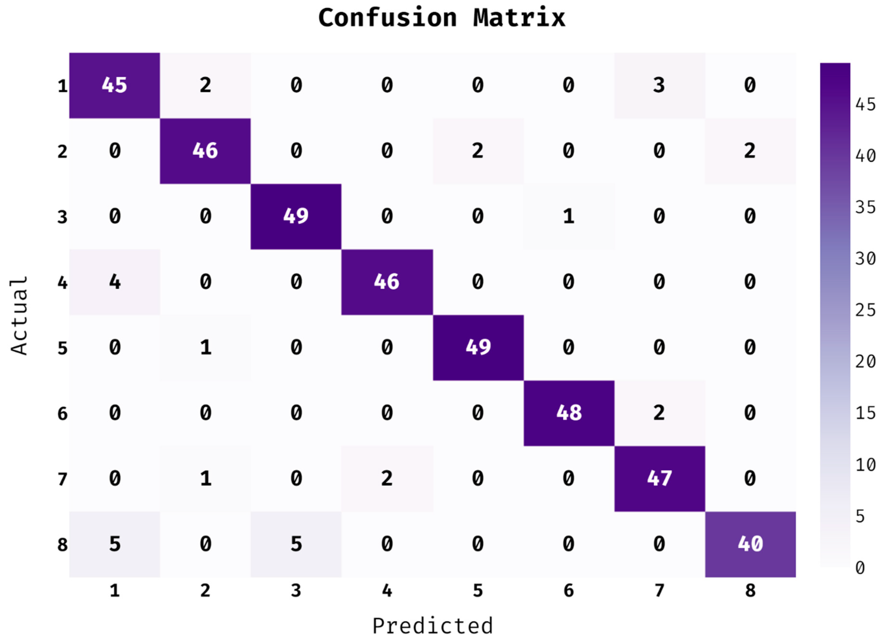
The experimental result analysis of the CIWHO-ORC technique was examined under traffic light datasets, which comprised of eight types of different traffic lights. Figure 5 illustrates the confusion matrices produced by the CIWHO-ORC technique for recognizing different traffic lights. The CIWHO-ORC technique identified 45 images under class 1, 46 images under class 2, 49 images under class 3, 46 images under class 4, 49 images under class 5, 48 images under class 6, 47 images under class 7, and 45 images under class 8.

Table 6. Traffic signal classification results of CIWHO-ORC technique.

Methods	Accuracy	TNR	F-Score	MCC
Green Light (1)	0.9650	0.9743	0.8654	0.8461
Green Left (2)	0.9800	0.9886	0.9200	0.9086
Green Right (3)	0.9850	0.9857	0.9423	0.9346
Green Up (4)	0.9850	0.9943	0.9388	0.9305
Red Light (5)	0.9925	0.9943	0.9703	0.9661
Red Left (6)	0.9925	0.9971	0.9697	0.9655
Red Right (7)	0.9800	0.9857	0.9216	0.9103
Red Up (8)	0.9700	0.9943	0.8696	0.8569
Average	0.9812	0.9893	0.9247	0.9148

offers the overall traffic signal classification results obtained by the CIWHO-ORC technique. The results reported that the CIWHO-ORC technique effectively identified distinct classes of traffic signals. For instance, with a green light (1), the CIWHO-ORC technique gave an accuracy of 0.9650, a TNR of 0.9743, an F-score of 0.8654, and an MCC of 0.8461. Meanwhile, with a green right (3), the CIWHO-ORC technique provided an accuracy of 0.9850, a TNR of 0.9857, an F-score of 0.9423, and an MCC of 0.9346. Eventually, with the red light (5), the CIWHO-ORC technique obtained an accuracy of 0.9925, a TNR of 0.9943, an F-score of 0.9703, and an MCC of 0.9661. At last, with a red light (8), the CIWHO-ORC technique gave an accuracy of 0.9700, a TNR of 0.9943, an F-score of 0.8696, and an MCC of 0.8569.

Result Analysis on KITTI MOD Dataset

Finally, the result analysis of the CIWHO-ORC technique takes place on the KITTI MOD dataset [24,25,26,27,28], which includes 5997 static vehicles and 2383 dynamic ones labeled.

Table 7. Classification results of CIWHO-ORC technique under KITTI MOD dataset.

Class Labels	Precision	Recall	F-Score
Static-Van	0.895	0.795	0.835
Static-Car	0.961	0.714	0.792
Dynamic-Van	1.000	0.723	0.791
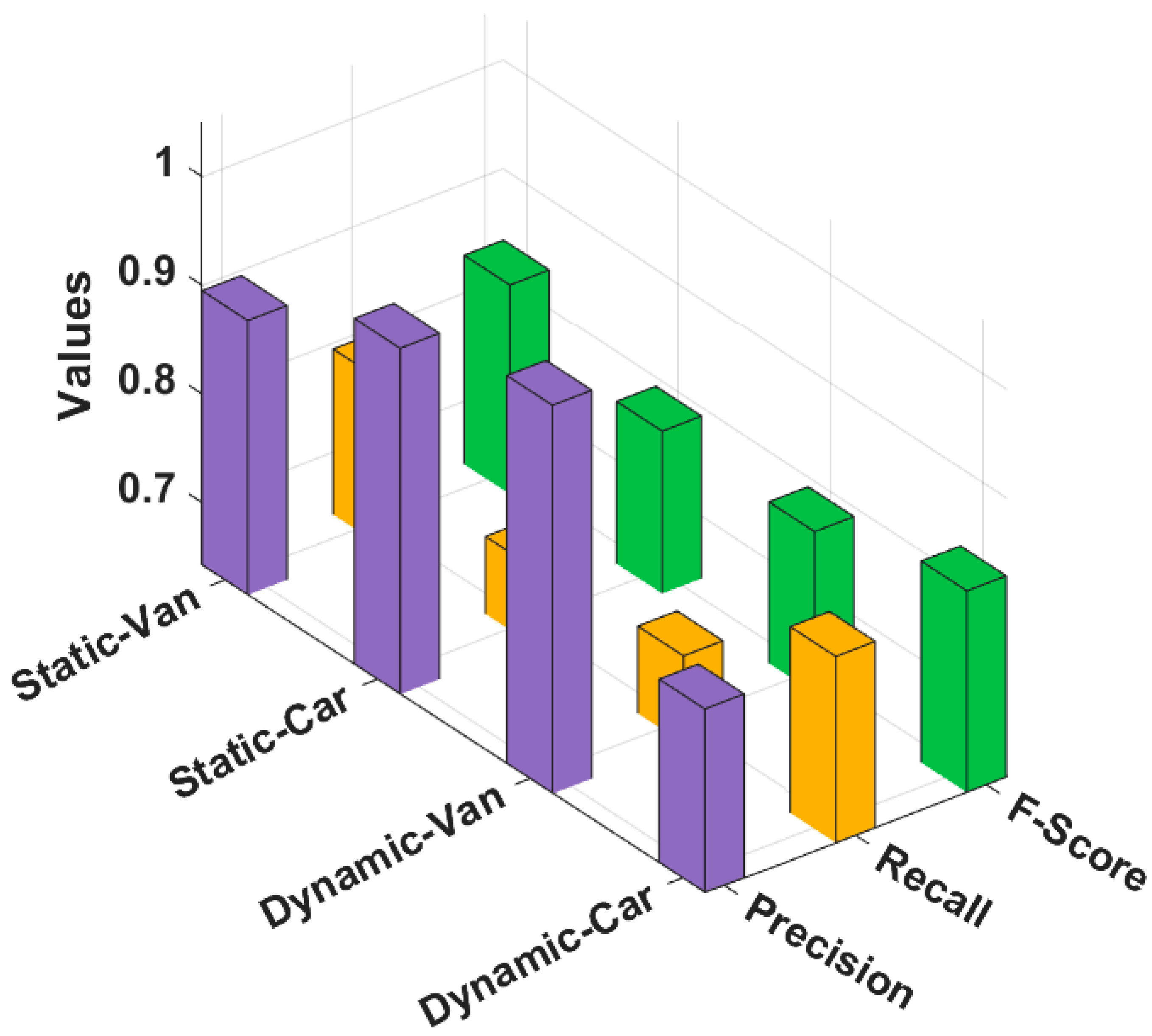
Dynamic-Car	0.812	0.814	0.828

and Figure 6 provide brief classification results of the CIWHO-ORC technique under distinct classes. The results stated that the CIWHO-ORC technique has accomplished enhanced classifier results under all classes. For example, under the static-van class, the CIWHO-ORC technique resulted in a precision of 0.895, a recall of 0.795, and an F-score of 0.835. At the same time, under the static-car class, the CIWHO-ORC technique attained a precision of 0.961, a recall of 0.714, and an F-score of 0.792. Likewise, under the dynamic-van class, the CIWHO-ORC technique resulted in a precision of 1.000, a recall of 0.723, and an F-score of 0.791. Finally, under the dynamic-car class, the CIWHO-ORC technique has resulted in a precision of 0.812, a recall of 0.814, and an F-score of 0.828.

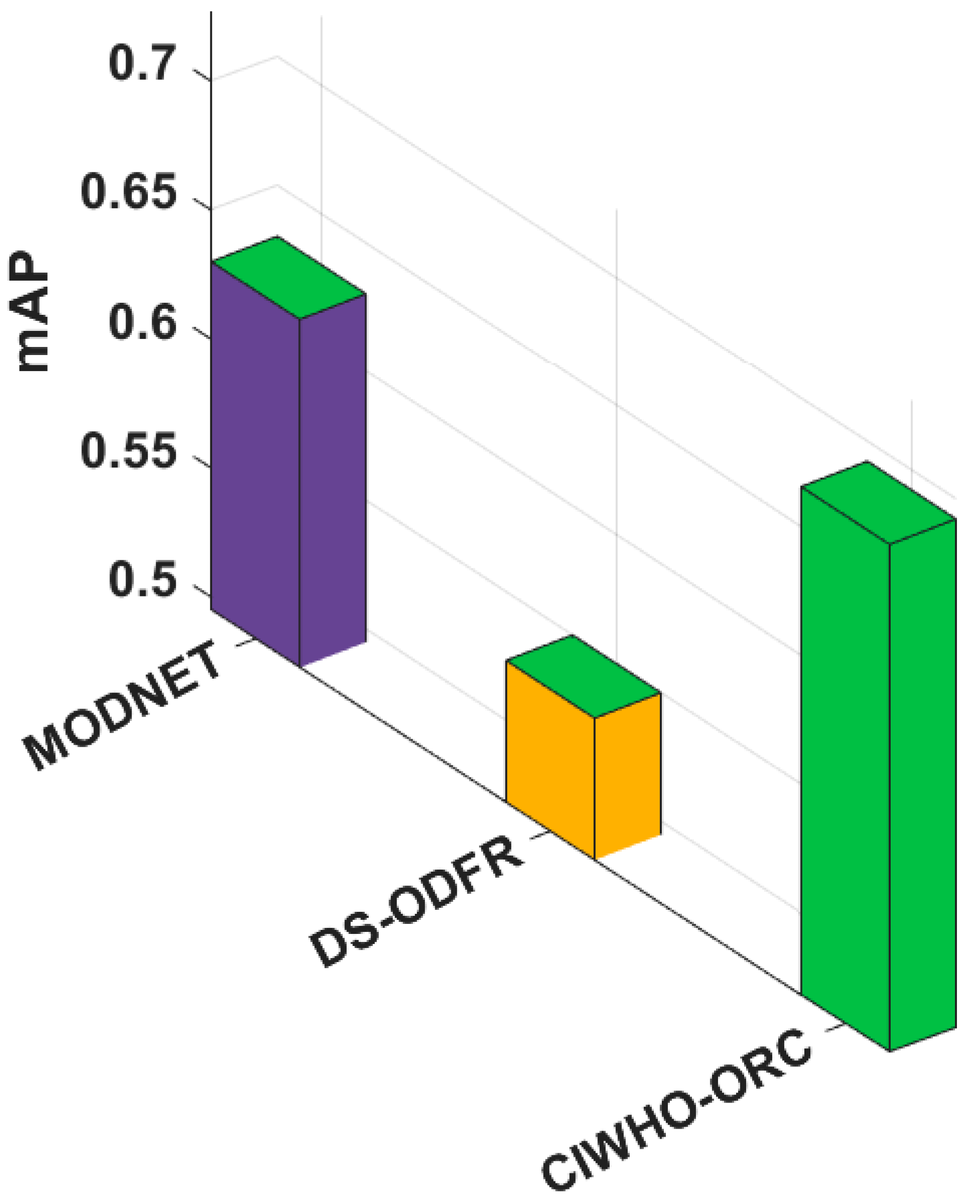
In order to report the improved outcomes of the CIWHO-ORC technique, a comparative analysis with existing techniques takes place in terms of the mAP in

Table 8. Comparative mAP analysis of CIWHO-ORC technique under KITTI MOD dataset.

Methods	mAP
MODNET	0.630
DS-ODFR	0.550
CIWHO-ORC	0.692

and Figure 7 [29]. The experimental results indicated that the DS-ODFR technique achieved the least outcome with an mAP of 0.550.

The MODNET technique obtained a slightly enhanced performance with an mAP of 0.630. However, the CIWHO-ORC technique resulted in effective detection results with a maximum mAP of 0.692. From the result analysis, it can be verified that the CIWHO-ORC technique has the ability to detect and classify objects under several conditions.

5. Conclusions

In this study, a novel CIWHO-ORC technique was developed to effectively identify the presence of multiple static and dynamic objects, such as vehicles, pedestrians, signboards, etc., for autonomous driving systems. The CIWHO-ORC technique encompasses two major processes, namely multi-scale Faster RCNN-based object detection and OSRR-based classification. Additionally, the KH and WHO algorithms were applied to tune the parameters involved in the multi-scale Faster RCNN and OSRR techniques, respectively. The simulation analysis of the CIWHO-ORC technique was examined against benchmark datasets, and the results were inspected under several evaluation measures. Detailed comparative results demonstrated the promising outcome of the CIWHO-ORC technique’s maximum detection accuracy of 0.9788 on the test of the Bdd100k dataset. In future, the proposed model can be extended to identify dangerous objects and the intended actions of detected pedestrians on roads. In addition, the proposed model can be tested on a large-scale heterogeneous dataset in the future. Moreover, the proposed model can be implemented in a real-time environment.