Article

Statistical Power Analysis in Reliability Demonstration Testing: The Probability of Test Success

1
Institute of Machine Components, University of Stuttgart, 70569 Stuttgart, Germany
2
Robert Bosch GmbH, 72703 Reutlingen, Germany
*
Author to whom correspondence should be addressed.
Appl. Sci. 2022, 12(12), 6190; https://doi.org/10.3390/app12126190
Submission received: 2 June 2022 / Revised: 14 June 2022 / Accepted: 16 June 2022 / Published: 17 June 2022
(This article belongs to the Special Issue Reliability Techniques in Engineering Projects)

Abstract

:
Statistical power analyses are used in the design of experiments to determine the required number of specimens, and thus the expenditure, of a test. Commonly, when analyzing and planning life tests of technical products, only the confidence level is taken into account for assessing uncertainty. However, due to the sampling error, the confidence interval estimation varies from test to test; therefore, the number of specimens needed to yield a successful reliability demonstration cannot be derived by this. In this paper, a procedure is presented that facilitates the integration of statistical power analysis into reliability demonstration test planning. The Probability of Test Success is introduced as a metric in order to place the statistical power in the context of life test planning of technical products. It contains the information concerning the probability that a life test is capable of demonstrating a required lifetime, reliability, and confidence. In turn, it enables the assessment and comparison of various life test types, such as success run, non-censored, and censored life tests. The main results are four calculation methods for the Probability of Test Success for various test scenarios: a general method which is capable of dealing with all possible scenarios, a calculation method mimicking the actual test procedure, and two analytic approaches for failure-free and failure-based tests which make use of the central limit theorem and asymptotic properties of several statistics, and therefore simplify the effort involved in planning life tests. The calculation methods are compared and their respective advantages and disadvantages worked out; furthermore, the scenarios in which each method is to be preferred are illustrated. The applicability of the developed procedure for planning reliability demonstration tests using the Probability of Test Success is additionally illustrated by a case study.

1. Introduction

Expenditures play an essential role in planning reliability demonstration tests. Resources are finite, and must be used in the most efficient way. Reliability demonstration tests should therefore use expenditures in such a way that they have the greatest effect, that is, the maximum promise of successful reliability demonstration.

1.1. Motivation

Determining the required sample size for the identification of relevant effects is an essential component of the frequentist design of experiments (DOE) methodology framework [1]. Statistical power analyses are employed to determine the sample size in order to identify the technologically relevant effects with a defined probability by using the estimated variance of the data [2]. In general, the type II error is used alongside the type I error, and should be kept as small as possible. The type II error is the complement to the statistical power; therefore, it represents the risk of not detecting existing effects below a certain threshold value while performing a test. For technical products, which have to endure a certain service life before they fail, such concepts lack implementation and application. From a life test perspective on such products, a type II error is made in a test if the test result does not demonstrate the required reliability when the product actually does meet the requirement in reality. By making use of the power, the planning of expenditures becomes possible; additionally, test configurations can be identified which cannot be realized from a practical point of view due to a too-high sample size requirement.

1.2. Assessment of Recent Work

Several scientific domains other than reliability engineering have used power analysis for years. Here, the focus often is on the evaluation of statistically significant effects in relation to the sample size and the determination of rules for termination in the event of a low probability of success in a study (see, e.g., [3,4,5,6]). In quality engineering, statistical power analysis is used in order to efficiently deal with lot acceptance tests and production parameter assessment [7]. In the reliability domain and within the scope of life testing of technical products, a holistic approach for power analyses has not been established for successful demonstration of reliability targets considering all possible test types. The uncertainty of the tested sample is assessed primarily by means of the confidence level, which solely addresses the type I statistical error [8]. Several tested samples of the same size result in different confidence intervals due to sampling variability [9]. Therefore, it is not sufficient to calculate the sample size required to demonstrate the reliability target solely by means of the confidence level; e.g., see [8]. A simple transfer of these power analyses to the life testing framework is challenging, as state-of-the-art analytic power analyses are only permissible for normally distributed residuals [1]. This does not apply to life data, which are usually Weibull or log-normally distributed [9]. Further challenges in life testing are the various test types and configurations, such as time- or failure-censored tests with or without load acceleration. For accelerated life tests, a life-stress model must be determined to demonstrate reliability for field load. It is possible to carry out life tests at different system levels, as well, such as at the component or subsystem level, which brings additional challenges. These aspects must be considered for the application of power analyses when planning reliability tests. The metric for the assessment of the accuracy must contain information as to whether a life test is capable of demonstrating a required reliability R r with required lifetime t r and confidence level C r . Due to the randomness of the process and the sole frequentist nature of reliability targets, it is necessary to deal with probabilities, and statistical power (as a statistical variable) must therefore be transferred to the domain of reliability test planning in order to be interpreted as the probability of a successful reliability test. The challenges are the generalization of the target variable in order for different test strategies to be dealt with and compared to each other, and performing the calculation in an efficient way.
In practical applications, success run tests (SR tests, called zero-failure tests or failure-free tests) are often used for reliability demonstration because the required sample size and reliability can easily be obtained using the binomial distribution [10]. Due to the equation only representing a significance test, only the confidence level C is considered. Over the past decades, there has been great effort to reduce the required sample size for the SR test by using Bayes’ rule [11], as its testing effort is quite high, especially for high reliability requirements, and even higher if failures occur during testing. Although the concept of a reliability demonstration has to be based on a frequentist view, due to the confidence level which is requirend and to be demonstrated Bayes’ rule continues to be used for aggregation of additional information. However, the demonstration is carried out solely using the frequentist confidence level instead of a credibility interval or other related concepts. Methods described by Beyer and Lauster [12,13], Guida and Pulcini [14], Kleyner et al. [15,16], Krolo [17,18,19], Savchuk and Martz [20], and Grundler et al. [21] use reliability information from similar products such as predecessors. The resulting posterior density can be used to carry out the reliability demonstration. For planning purposes, however, assuming a successful test (no failures occur), the posterior density can be used to calculate the required sample size for the test. These procedures differ partly in the determination of the prior distribution and in the proportion of prior knowledge used. Bayer and Lauster [12] do not use a distribution of reliability in their method, instead using a nominal reliability value with a fixed confidence level of 63.2% of the predecessor product. Grundler et al. [13] remove this restriction, permitting variable confidence levels as well as accelerated tests. When employing the Kleyner and Krolo methods [15,16], failure distributions can be used as prior knowledge. Kleyner et al. [15] use a beta and a uniform distribution, which are weighted according to the similarity of the products. The method introduced by Krolo [17,18,19] allows prior knowledge from different populations and sources, such as test results and field data, to be used. Additionally, Grundler’s approach [13] permits the use of prior knowledge from fatigue and lifetime calculations. The main challenge of these methods is the primarily subjective assessment of the similarity of two products, which makes the reliability demonstration vulnerable in the event of doubt [22]. Although Hitziger [23] describes approaches for determining similarity, uncertainty remains in the application of these methods, because even very small changes in the production process can lead to profound changes in failure behavior. However, it is difficult to objectively attest a certain similarity of the products in this case. None of the methods for reducing the required sample size of SR tests takes the type II error into account for test planning; in fact, only the type I error is considered by the confidence level. Consequently, no statement on the result of the test is possible, which means that no estimate can be made about either the success of the test nor about a successful reliability demonstration. However, some approaches do exist which address the issue of the two types of risks during zero-failure testing. Lu et al. [24] use the Bayesian approach presented in [25] in order to assign a success probability to the failure-free reliability demonstration test. However, they make use of an indifference region, which uses an interval of reliability values instead of a single reliability target. This results in a decoupling of the planning and assessment aspects of the test from the reliability target. The reliability target should be very much integrated as an integral part of reliability demonstration test planning. The very similar approach in [26] uses the assurance of [25] in order to calculate a probability for the outcome of the SR test. The main drawback, other than the use of two reliability values instead of one reliability target, is the sole focus on the SR test. No other test types can be analysed using these approaches and no comments about lifetime ratios or acceleration factors are made. A transfer to the context of failure-based tests is not trivial, as these approaches rely on the binary classification on which the SR test is based. Wilson and Farrow [27] propose a Monte Carlo simulation (MCS) for assurance calculation of failure-based tests. However, the computational burden is very high, and the indifference region is used. The problem with these Bayesian approaches of [24,25,26,27] is that they result in a credibility interval instead of a confidence interval, which is required for a reliability demonstration with a required confidence level. In addition, the indifference region does not comply with the demonstrated reliability target.
The literature contains several approaches that address the optimization of end-of-life testing (EoL test, called failure-based tests) strategies in a frequentist manner. However, the type II error is neglected within most approaches. Several approaches that do consider the type II error use it in a different context, e.g., as an economic aspect in the sense of customer risk, or limit their analysis to a specific test type, such as sudden death tests (SD tests). In the work of Guo et al. [28], the accuracy of an uncensored EoL test is discussed. As an assessment criterion, the confidence interval width is used as a ratio of upper and lower confidence bounds at a certain lifetime quantile. MCS are used to determine the required sample size, which results in the desired confidence interval width for a Weibull distribution stemming from prior knowledge. Arizono et al. [29] present a method to determine an SD test configuration that allows a mean time to failure (MTTF) to be estimated most economically through MCS. In a certain parameter space of the Weibull shape parameter, sample size, and inspection lot size, a decision is made as to whether the inspection lot is accepted or rejected. The Weibull evaluation is limited to the MTTF, whereby smaller failure probabilities might be more interesting in practical application. Huang and Wu [30] focus their work on time-censored EoL test plans, which are approximated using exponential distributions, and in which test specimens are observed in intervals. The entire approach is limited to exponential distribution and time-censored tests, which results in limited applicability. Vlcek et al. [31] compare the SD test with non-censored, time-censored, and failure-censored EoL tests with regard to time-saving potential. Various test configurations are generated using MCS. The average duration of failure-censored tests is discussed by Hsieh [32]. The expected test time values are calculated and compared using a binomial distribution. This means that the time benefits of failure-censored tests, which depend on the Weibull shape parameter, the sample size, and the censoring proportion, can be worked out. Tsai et al. [33] evaluate failure-censored tests under limited test infrastructure. The investigated influencing variables are the sample size, censoring proportion, number of sequential tests, and the acceptance probability of an inspection lot on the basis of a failure distribution specified as already known.

1.3. Research Gaps

Based on the preceding discussion, it can be concluded that more work remains to be carried out for the optimization of individual EoL and SR test strategies. In existing approaches, the focus is often on one target variable for a single test type. A metric and a procedure for planning reliability demonstration tests with consideration of all available test types and boundary conditions in the required frequentist manner does not yet exist. The research gaps can be thus summarizes as follows:
  • A metric for objectively assessing reliability tests based solely on their ability to demonstrate the frequentist reliability target must be established;
  • A holistic approach to assessing all possible reliability tests needs to be developed;
  • A procedure for efficient reliability demonstration test planning considering all possible reliability tests needs to be worked out;
  • The calculation effort involved in reliability test planning needs to be reduced.
These gaps are addressed and sequentially worked out in the rest of this manuscript.

1.4. Outline

The manuscript is organized as follows. First, the Probability of Test Success is introduced as the statistical power of a reliability demonstration test. The necessary hypotheses are formulated, mathematically defined, and illustrated. In Section 3, calculation methods for the Probability of Test Success are established. Here, four methods are introduced. The general method is capable of calculating the Probability of Test Success in all possible scenarios. It can easily be adapted thanks to the Bootstrap approach used here. The analytic method for SR tests enables a very fast and easily implementable calculation for failure-free tests, whereas the analytic and approximate calculation method for failure-based tests allows for an equally quick calculation of the Probability of Test Success of failure-based tests using the asymptotic properties of several statistics. Additionally, a calculation method which does not rely on the concept of the statistical power, and instead simulates the testing scheme, is explained. The advantages of these methods are worked out and compared to each other in Section 4. In order to illustrate the use and effect of the concept and the procedure for test planning of reliability demonstration tests, Section 5 uses a case study to demonstrate the holistic view one is able to obtain by employing the Probability of Test Success. This is additionally illustrated by the example of the monetary aspects of the case study, which concerns a high-voltage battery. Section 6 discusses the major work, contributions, challenges, and results of the presented approach and concludes the findings with recommendations for future works.

2. Probability of Test Success

Product development, with all its calculations and the design of the product itself, should ensure both the actual fulfillment of the required functions and the reliability requirements under the corresponding field conditions [10,34]. Without evidence, the requirement cannot be regarded as fulfilled, whereas a hypothesis about the non-fulfillment can be established. This hypothesis must be either rejected or accepted by conducting a reliability test. Therefore, a reliability demonstration test can be regarded as a hypothesis test. The reliability requirement is formulated as a required lifetime with a certain reliability and confidence level. The estimated lifetime quantile of the test, t R r , at the required reliability, R r , has to be greater than or equal to the required life quantile, t r . As a statistical test is only able to provide evidence towards the rejection of a hypothesis that states the absence of a certain phenomenon of interest [35,36,37], the null hypothesis, H 0 , represents the non-fulfillment of the reliability requirement and is to be rejected. Because the power of the test corresponds to the detection of the fulfillment of the requirement, the alternative hypothesis, H 1 , represents the reliability requirement in terms of the lifetime. Therefore, the hypotheses to be used in a reliability demonstration test are defined as the following [38,39,40,41]:
H 0 : t R r < t r
H 1 : t R r t r
As a fulfillment of the reliability requirement cannot be assumed without evidence of a proper demonstration by means of a successful test, the very common terms of producer risk and consumer risk in quality engineering [42,43,44] are not applicable here in the classical sense of type I and type II error [37,40]; these terms are only meaningful if a manufacturing issue is at hand. For example, testing of the production parameters of a production line always endeavors to avoid deviations and effects from the specified parameter space. However, the observed effect of interest in a reliability demonstration test is the lifetime, and therefore, the desired effect.
The significance level at which the null hypothesis is to be rejected is determined by the permitted type I error, α , which is the probability for the null hypothesis to be rejected even though the null hypothesis actually holds true. The confidence level, C, of a reliability test corresponds to the complement of the permitted significance level, α , as it describes the probability that the reliability test rightly accepts the null hypothesis when the reliability requirement ( t r , R r , C r ) is actually not met by the product according to the test data. Therefore, the required confidence level, C r , is able to assess and ensure that the obtained reliability statement is indeed true. As a great variety of test plans are available to obtain a reliability statement, the problem of choosing the correct and most promising reliability test strategy arises. In order to assess the different test strategies, an additional assessment criterion is needed. In contrast to the approach of hypothesis tests, reliability tests do not generally consider the type II error, which describes the probability β that the null hypothesis H 0 is wrongly accepted. The type II error depends on the sample size, the effect size (the actual value of the lifetime quantile) and failure distribution, the sampling variance, and the desired significance level. The complement of the type II error, β , is termed the statistical power of the test, and describes the probability that the test correctly rejects the null hypothesis for a certain effect size [35]. In the context of reliability test planning, this power describes the probability of a test demonstrating the reliability requirement. As the hypothesis of reliability demonstration tests stay the same, as defined in (1) and (2), the statistical power of a reliability demonstration test is called the Probability of Test Success, P ts . Therefore, merely considering a confidence level ( 1 α ) in reliability test planning is not sufficient, as the analysis of the applicability of the test ( 1 β ) to the individual scenario is neglected [38,39,40,45,46,47]. Because the power of a test, and therefore the Probability of Test Success, has to be calculated for a specific effect size [35], and because the probability of detecting an effect changes with a change in the effect size, a measure of the effect size has to be established for reliability tests. For this purpose, the safety distance, s, of the product is used, as introduced by Dazer et al. [46]. The safety distance describes the distance of the required lifetime, t r , to the actual lifetime of the product, t p , in accordance with prior knowledge about the failure distribution, and is defined as follows:
s 1 t r t p
where t p is the lifetime with the required reliability in accordance with the prior knowledge and t r is the required lifetime at the required reliability. The safety distance, s, is equal to zero if the prior knowledge states that the required lifetime is equal to the actual service life of the product. Using this metric, the effect size, Δ , can be formulated as follows:
Δ t p t r = s · t p
In order to calculate the confidence level, C, as well as the P ts , the distributions of the test statistic under validity of the null and the alternative hypothesis must be obtained. Using the safety distance from (3) as well as the effect size from (4), the test statistic, τ , of reliability demonstration tests is defined as
τ t R r t r .
This is because it measures the distance from the lifetime quantile of the test to the expectation of it under validity of the null hypothesis ( τ = 0 for t R r = t r ) and the prior knowledge about the failure distribution.
The null distribution f H 0 ( τ ) and alternative distribution f H 1 ( τ ) of the test statistic are defined by the prior knowledge of the failure distribution and the sampling scheme of the test. Regarding this approach, it can be concluded that prior knowledge of the failure distribution is indispensable for statistically profound planning of reliability tests, as the actual effect size of the product is determined by this information. The distribution of the test statistic under validity of the alternative hypothesis (alternative distribution f H 1 ( τ ) ) can be obtained by shifting the confidence distribution [48] of the calculated test statistic under H 1 by the required lifetime, t r . The confidence distribution is dependent on the sample size and the test to be analyzed as well as on the failure distribution, and can be calculated by means of an MCS and a maximum likelihood estimation (MLE), for example. The distribution of the test statistic under validity of the null hypothesis (null distribution f H 0 ( τ ) ) can be obtained through the same procedure, although in contrast with the alternative distribution it must be calculated via the failure distribution, which is valid under H 0 ; therefore, s = 0 (effect size of zero, Δ = 0 ). Where a Weibull distribution is concerned, the shape parameter should be kept the same in order to maintain the characteristic of the failure mode at hand (see [10]), whereas the scale parameter should be adjusted accordingly. Taking the null distribution f H 0 ( τ ) , the significant effect size, Δ crit , can be calculated in accordance with the required confidence, C r . Then, the alternative distribution f H 1 ( τ ) provides the Probability of Test Success P ts , that is, the statistical power of the test type to be analyzed. The required equations are as follows:
C = 1 α = Δ crit f H 0 ( τ ) d τ
P ts 1 β = Δ crit + f H 1 ( τ ) d τ
The distributions can be pdfs or probability mass functions (pmfs) if an MCS is used to obtain them. Therefore, the Probability of Test Success  P ts is defined via (1)–(7).
The dependencies between the hypotheses, the confidence level, and the P ts are shown in Table 1, and the two distributions of (4) and (5) are shown in Figure 1 alongside the relevant parameters.

3. Calculation of the Probability of Test Success

In order to calculate the P ts for the specific reliability test configuration at hand, the distributions of the test statistic, τ , under H 0 and H 1 need to be calculated, as do the two integrals of (6) and (7). Four different methods are presented here:
A.
A general calculation method
B.
An analytic and exact calculation method for SR tests
C.
An analytic and approximate calculation method for failure-based tests
D.
A calculation method using test simulation.
The general calculation method uses a bootstrap approach and enables the calculation of P ts for all possible test scenarios in the desired accuracy. The analytic and exact calculation for SR tests makes use of the binomial approach of the SR test. The approximate method for failure-based tests allows the P ts for EoL tests to be analytically calculated using the asymptotic properties of the sample quantile and the MLE. The calculation method, which simulates the reliability test, abstains from the hypothesis testing framework and solely relies on the law of large numbers.

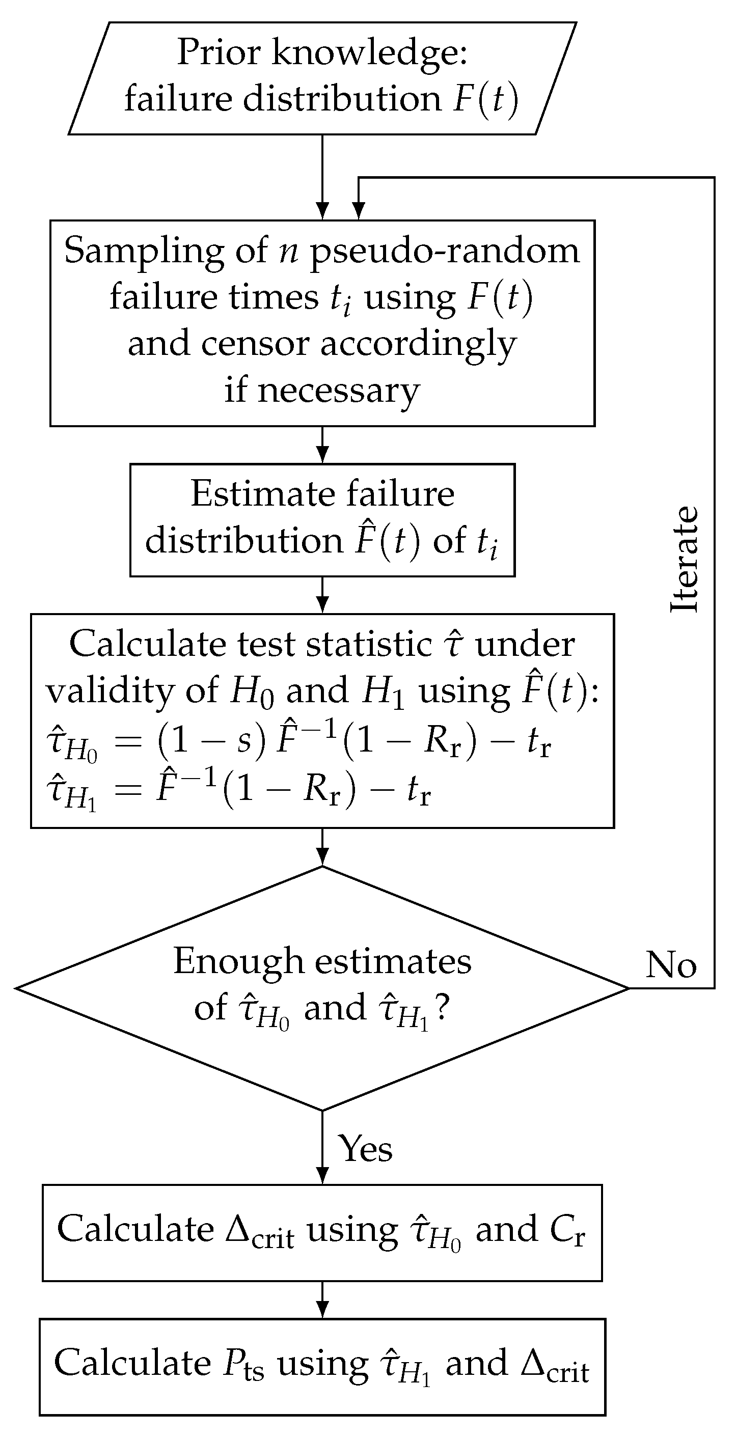
3.1. General Calculation Procedure

Due to the possibly very complex sampling schemes and the great variety among reliability tests and their configurations, any general calculation procedure must be very flexible. In order to guarantee such flexibility, a bootstrap [49] approach is used here, as it does not require analytical effort or equation solving prior to the actual calculation taking place. The bootstrap approach is used to estimate the sampling distributions of (6) and (7) from Figure 1. Because f H 0 and f H 1 are obtained in empirical form from the bootstrap iterations and used in a parameter-free way, the variance and the entire shape and all of the statistical moments [10,50] of the distributions are captured. Therefore, no assumption as to the distribution type has to be made.

3.1.1. General Calculation for Failure-Based Tests

For failure-based tests, such as EoL tests or censored EoL tests, the first step of the bootstrap is to draw n pseudo-random failure times from the failure distribution F ( t ) available from the prior knowledge. The sample size n and the sampling behavior of these failure times must be the same as the reliability test for which P ts is to be calculated. If censoring of the failure times is prevalent in the test, it must be reflected here in the same way. The failure distribution F ^ ( t ) of this bootstrap sample is then estimated by, e.g., a maximum likelihood estimation (MLE) [51,52], and the lifetime at the required reliability t ^ R r is calculated. Because the failure distribution of the prior knowledge determines the effect size Δ and is linked to the alternative hypothesis, H 1 (if s > 0 ), subtracting the required lifetime t r from this value yields a value of the test statistic under validity of H 1 as follows:
τ ^ H 1 = t ^ R r t r = F ^ 1 ( 1 R r ) t r
The test statistic under validity of the null hypothesis H 0 is obtained in the same way; however, the failure distribution has to follow H 0 , which means that the safety distance must be negative or equal to zero ( s 0 ). If the failure distribution under H 0 is known and satisfies s 0 , it should be used. However, in most practical applications, only prior knowledge about the products’ performance is known, which corresponds to H 1 . In order obtain the failure distribution such that s = 0 , which translates to t p = t r , the failure times of F ( t ) can be multiplied by ( 1 s ) . This multiplicative transformation ensures a preservation of the shape of the failure distribution, F ( t ) , which corresponds to the failure mechanism itself. This is in accordance with the shape parameter of a Weibull distribution being tied to the failure mechanism [10]. For the hypothesis test to work, the failure mechanism has to stay the same. Using the already-drawn bootstrap samples of t ^ R r from F ( t ) , the following equation yields the test statistic under validity of the null hypothesis, H 0 :
τ ^ H 0 = ( 1 s ) t ^ R r t r = t r · F ^ 1 ( 1 R r ) F 1 ( 1 R r ) 1
where the value of s with t p calculated as t p = F 1 ( 1 R r ) of the prior knowledge is used. Multiple iterations of sampling from the failure distribution of the prior knowledge, estimating t ^ R r , and transforming the values to obtain the distributions of τ ^ H 1 and τ ^ H 0 enable to use the law of large numbers [53] for calculating the integrals of (6) and (7). The value of Δ crit of (6) is calculated by
C r = ! Number   of   τ ^ H 0 Δ crit Total   number   of   iterations .
Using the calculated value of Δ crit , the P ts of failure-based tests can be calculated using
P ts = Number   of   τ ^ H 1 Δ crit Total   number   of   iterations .
Because the location of the distributions of the obtained test statistics, τ ^ H 0 and τ ^ H 1 , are tied to the hypothesis ( s 0 and s > 0 ) and are eventually subject to bias errors due to the estimator of the quantiles (e.g., MLE bias), the two distributions are shifted such that median ( τ ^ H 0 ) = 0 and median ( τ ^ H 1 ) = t p t r . In this way, the bootstrap procedure only estimates the variance and shape of the sampling distributions. In order to calculate the P ts of a censored EoL test, the samples drawn during the bootstrap must be censored accordingly. If, e.g., an MLE is used for the estimation of the failure distribution of the bootstrap sample, the censoring can be accounted for. The general procedure for calculating the P ts of an EoL test is shown in Figure 2. In this procedure, the number of iterations should be kept as high as possible, as the results become more accurate with higher iteration numbers. However, more iterations equal higher computational effort, which is why 10,000 iterations should be sufficient for most applications. Ideally, for each use case a convergence analysis can be made in which the number of iterations in which a sufficient calculation accuracy is achieved can be examined, cf. Section 4.1.

3.1.2. General Calculation for the Success Run Test

For calculating the P ts for SR tests the procedure is much simpler, as only failures have to be counted in order to attest a success. Using the same bootstrap samples drawn from F ( t ) , the P ts of an SR test with a maximum of k failures allowed during testing is calculated by
P ts = Number   of   bootstrap   samples   with   κ k Total   number   of   iterations
with κ being the number of failures occurring in one sample.

3.2. Exact Calculation for the Success Run Test

While the aforementioned procedure for calculating P ts can be used for all test types, the SR test enables an exact calculation in a closed form and no bootstrap procedure is required. As an SR test does not yield an estimation of the lifetime, rather, a confidence distribution of the reliability at the required lifetime t r in the form of a binomial distribution, the hypothesis in (1) and (2) can be reformulated as follows:
H 0 : R ( t r ) < R r ( t r )
H 1 : R ( t r ) R r ( t r )
Here, the demonstrated reliability, R ( t r ) , at the required lifetime, t r , is the deciding value for a successful demonstration ( H 1 ) or a failed one ( H 0 ). With a sample size n of the SR test, the achieved confidence level C of the required reliability R r can be calculated using the following binomial distribution [10]:
C = 1 i = 0 k n i · R r n i · 1 R r i
That is, if during the test time equal to the required lifetime t r a maximum of k specimens fail. The binomial approach assumes that the parameter of the binomial distribution’s success rate is equal to the complement of the required reliability, R r , which corresponds to the null hypothesis of (13) (marginal case of s = 0 ). Analogous to (15) as well as to the integrals of (6) and (7), the P ts of an SR test can be calculated analytically using the binomial distribution:
P ts = i = 0 k n i · R p n i · 1 R p i
Instead of the required reliability, the reliability at the required lifetime stemming from prior knowledge R p ( t r ) = 1 F ( t r ) is used as the complement of the success rate of the binomial distribution. If R p ( t r ) > R r ( t r ) , this corresponds to the alternative hypothesis of (14). Due to the relationship between the binomial distribution and the beta distribution (see e.g., [54]), Equations (15) and (16) can be written in terms of the beta distributions as follows:
C = R r 1 R n k 1 · ( 1 R ) k β n k , k + 1 d R
P ts = 0 R p R n k 1 · ( 1 R ) k β n k , k + 1 d R
where β ( A , B ) is the Euler beta function [55] and the resulting beta distributions both have the parameters A = n k and B = k + 1 , as the resulting confidence distribution of the SR test is determined only by the number of surviving n k and the number of failing specimens k. Because it is the same distribution, it is immediately apparent that P ts is the complement of the confidence as the product’s reliability approaches the required level ( P ts 1 C as R p R r or s 0 ). When planning the SR test, (15) is used to calculate the required sample size to meet the reliability requirement; hence, the sample size and the resulting distribution of reliability (beta distribution in (17) and (18)) are fixed by design. Because of this, the SR test can only achieve acceptable values for P ts (e.g., P ts > > 50 % ) if the product is over-sized to a great extent in terms of its reliability performance. The relevant distributions (see (17) and (18)) and parameters are shown in Figure 3.
In order to make use of an accelerated SR test and a test time other than the required lifetime, Equations (17) and (18) can be extended by an acceleration factor r and a lifetime ratio L R = t test t r (see [10]), as follows:
g ( R ) = R i = 1 n k r i L R , i b · j = 1 k 1 R r j L R , j b
C = R r 1 g ( R ) 0 1 g ( R ) d R d R
P ts = 0 R p g ( R ) 0 1 g ( R ) d R d R
The above makes use of an assumed Weibull distribution in which the shape parameter b is used to calculate the reliability at t r for the specimen with a different test time t test . The used integrands in (20) and (21) are no longer beta or binomial distributions, which is due to the missing exponent of the product on the right hand side of (19). However, they can be evaluated using numerical methods.

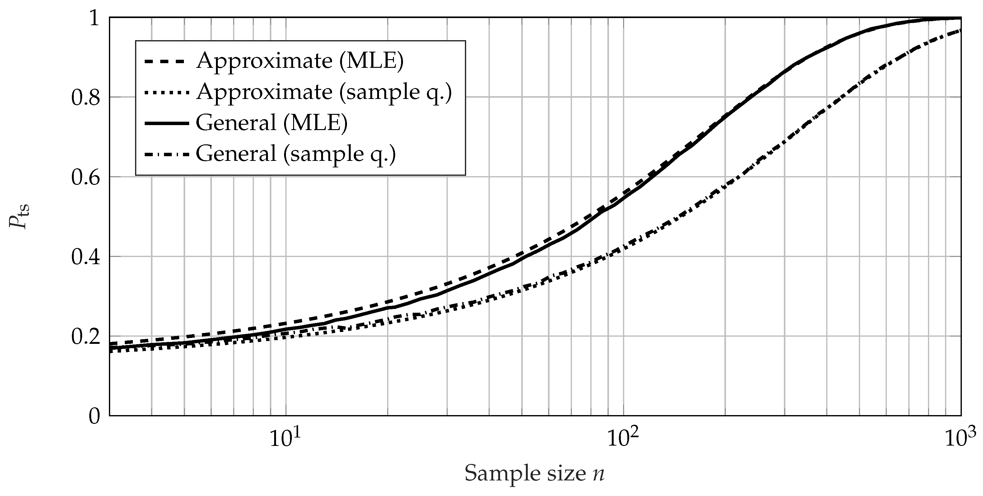
3.3. Approximate Calculation for Failure-Based Tests

The general method for calculating P ts using the bootstrap approach can become time- and resource-consuming if several different tests need to be analyzed and high accuracy is to be assured by a high iteration number. In order to enable a fast way of calculating P ts for failure-based tests (EoL test) in a way that is effortless to implement, an approximate calculation can be sufficient.
To obtain the distributions of τ H 0 and τ H 1 without an MCS or bootstrap, the central limit theorem (CLT) [56,57] can be used. Several statistical phenomena are normally distributed if the sample size is very large ( n ). If the sample size is finite, the normal distribution can nonetheless be used as a rough approximation. Using the CLT, the distribution of the sample quantile of a known distribution F ( t ) is normally distributed with mean μ and standard deviation σ , as follows [57,58]:
μ = F 1 ( q )
σ = q · ( 1 q ) n · f F 1 ( q ) 2
where q is the proportion of the quantile, F 1 ( q ) is the inverse of F ( t ) , f ( t ) is the pdf of F ( t ) , and n the sample size. To abbreviate (22) and (23), a normally distributed variable t can be written as t N ( μ , σ ) . Using the test statistic from (5) and the asymptotic behavior from (22) and (23), the approximated distributions τ H 0 and τ H 1 are the following normal distributions:
τ H 0 N 0 , R r · ( 1 R r ) n · f 0 ( t r ) 2
τ H 1 N t p t r , R r · ( 1 R r ) n · f t p 2
with f 0 ( t ) as the shifted pdf of the failure distribution of prior knowledge f ( t ) , such that it is valid under H 0 and t p = F 1 ( 1 R r ) . Where a Weibull distribution is concerned as the failure distribution of prior knowledge F ( t ) with scale parameter T and shape parameter b, the scale parameter of f 0 ( t ) can be calculated as
T 0 = ( 1 s ) T = t r t p T
while the shape parameter stays the same ( b 0 = b ). Using the CLT, (24) and (25), the Probability of Test Success P ts of an EoL test, if the lifetime quantile is determined by the empiric sample quantile, can be calculated approximately by
P ts 1 Φ Φ 1 C r ; 0 , R r · ( 1 R r ) n · f 0 ( t r ) 2 ; t p t r , R r · ( 1 R r ) n · f ( t p ) 2
with Φ ( x ; μ , σ ) being the cumulative distribution function (cdf) of the normal distribution at the value x with the parameters μ and σ . The inverse of the cdf of the normal distribution is Φ 1 ( q ; μ , σ ) .
The approximation of P ts uses the quantile of the sample instead of the quantile one would obtain using a distribution estimation. If a Weibull distribution and an MLE fit are concerned, a different approximation can be derived using the CLT and the likelihood, as well as the variance–covariance matrix together with a Taylor series expansion. Therefore, the P ts of the most common censored or uncensored EoL tests for Weibull distributions using an MLE estimation can be approximately calculated without the need for an MCS or bootstrap approach. The log-likelihood Λ of the two-parameter Weibull distribution is [8]
Λ ( T , b ) = ( n m ) ln ( b ) b ln ( T ) + i = 1 n m ( b 1 ) ln ( t i ) t i T b j = 1 m t j T b
with n m uncensored failure times t i and m right-censored failure times t j . The likelihood can be extended for left-censored or truncated as well as interval-censored failure times. The variance–covariance matrix V using (28) is the inverse of the Fisher information matrix, I [8]. Because I is symmetric and positive definite, its inverse and the matrix V can be calculated using
V = Var ( T ) Cov ( T , b ) Cov ( b , T ) Var ( b ) = I 1 = 2 Λ T 2 2 Λ T b 2 Λ b T 2 Λ b 2 1 = 1 det ( I ) 2 Λ b 2 2 Λ T b 2 Λ b T 2 T 2 V = 1 2 Λ T 2 2 Λ b 2 2 Λ T b 2 2 Λ b 2 2 Λ T b 2 Λ b T 2 Λ T 2
with
2 Λ T 2 = b T 2 n m ( b + 1 ) i = 1 n t i T b
2 Λ b 2 = m n b 2 i = 1 n m ln t i T 2 · t i T b + j = 1 m ln t j T 2 · t j T b
2 Λ T b = 2 Λ b T = m n T + 1 T i = 1 n 1 + b ln t i T · t i T b
and Var ( · ) and Cov ( · , · ) being the variance and covariance, respectively. The determinant of a matrix is det ( · ) . The summation in (30) and (32) is over both the uncensored failure times t i and the censored failure times t j . Only a single summation index i is used.
Using a linear Taylor series expansion [8,59], the variance of the MLE of the quantile function for the Weibull distribution t q = T ln ( 1 q ) 1 / b can be approximated by
Var ( t q ) = t q T 2 Var ( T ) + t q b 2 Var ( b ) + 2 t q T t q b Cov ( T , b ) = ln ( 1 q ) 2 / b Var ( T ) + T 2 b 4 ln ( ln ( 1 q ) ) 2 ( ln ( 1 q ) ) 2 / b Var ( b ) = 2 T b 2 ln ( ln ( 1 q ) ) ( ln ( 1 q ) ) 2 / b Cov ( T , b ) .
According to the asymptotic behavior of the MLE and the CLT under certain regularity conditions [8], the variable t q approximately follows a normal distribution; hence,
t q N T ln ( 1 q ) 1 / b , Var ( t q ) .
As no bootstrap and no MCS take place, the failure times in (30)–(32) can be calculated using the Weibull failure distribution F ( t ) of the prior knowledge. Using order statistics [54], the median of each failure time as a function of the sample size is
t i = F 1 F beta 1 ( 0.5 ; i , n i + 1 )
with F beta ( q ; A , B ) being the quantile function (inverse) of the beta distribution for quantile q and parameters A and B. The approximation of the median of the beta distribution of Benard [60], commonly used in rank regression [10], can be used here for a simpler implementation; hence, for a Weibull distribution with parameters T and b from prior knowledge,
t i T · ln 1 i 0.3 n + 0.4 1 / b i [ 1 , n ] .
Censored failure times can be generated using (35) or (36) and the corresponding censoring scheme. The established distribution of the sample quantile using the Weibull distribution of prior knowledge in (34) corresponds to the alternative hypothesis H 1 of (2). Therefore, the approximated distribution of the quantile t R r , H 1 under the validity of the alternative hypothesis is
t R r , H 1 N T ( ln ( R r ) ) 1 / b , σ H 1
with
σ H 1 = ( ln ( R r ) 2 / b Var ( T ) + T 2 b 4 ln ( ln ( R r ) ) 2 ( ln ( R r ) ) 2 / b Var ( b ) 2 T 2 b 2 ln ( ln ( R r ) ) ( ln ( R r ) ) 2 / b Cov ( T , b ) ) 1 / 2
using (29)–(32) with the parameters of the Weibull distribution from the prior knowledge as well as the failure times of (35) or (36) and q = 1 R r in (33). The distribution of the quantile t R r , H 0 under the validity of the null hypothesis has to use the shifted failure distribution with scale parameter T 0 of (26) and the calculated failure times using this shifted failure distribution and (35) or (36); accordingly,
t R r , H 0 N t r , σ H 0
with
σ H 0 = ( ln ( R r ) 2 / b Var ( T 0 ) + T 0 2 b 4 ln ( ln ( R r ) ) 2 ( ln ( R r ) ) 2 / b Var ( b ) 2 T 0 2 b 2 ln ( ln ( R r ) ) ( ln ( R r ) ) 2 / b Cov ( T 0 , b ) ) 1 / 2
where Var ( T 0 , b ) and Cov ( T 0 , b ) do not correspond to a different variable. Instead, (29) is used at the corresponding value of T 0 for T. Using these equations (from (37) to (40)), the P ts of a right-censored or uncensored EoL test in which the lifetime quantile is determined by distribution estimation via MLE can be calculated approximately by
P ts 1 Φ Φ 1 C r ; t r , σ H 0 ; T ( ln ( R r ) ) 1 / b , σ H 1 .
The approximations of (27) and (41) are approximate in several ways: first, (27) and (41) approximate the desired lifetime quantile distribution via a normal distribution, which does not hold for small sample sizes; second, the failure times used in (41) are approximated using order statistics in addition to the Benard approximation to the median of the beta distribution. However, the approximate calculations can be implemented effortlessly, as even most spreadsheet programs of the popular operating systems of personal computers have implementations of the normal distribution. The approximations are of benefit in cases where several test scenarios are required or dependencies over a large range of values need to be found. If the feasible space of test scenarios is narrowed down using the approximate calculation, the more accurate general method can be used to identify the optimal test.

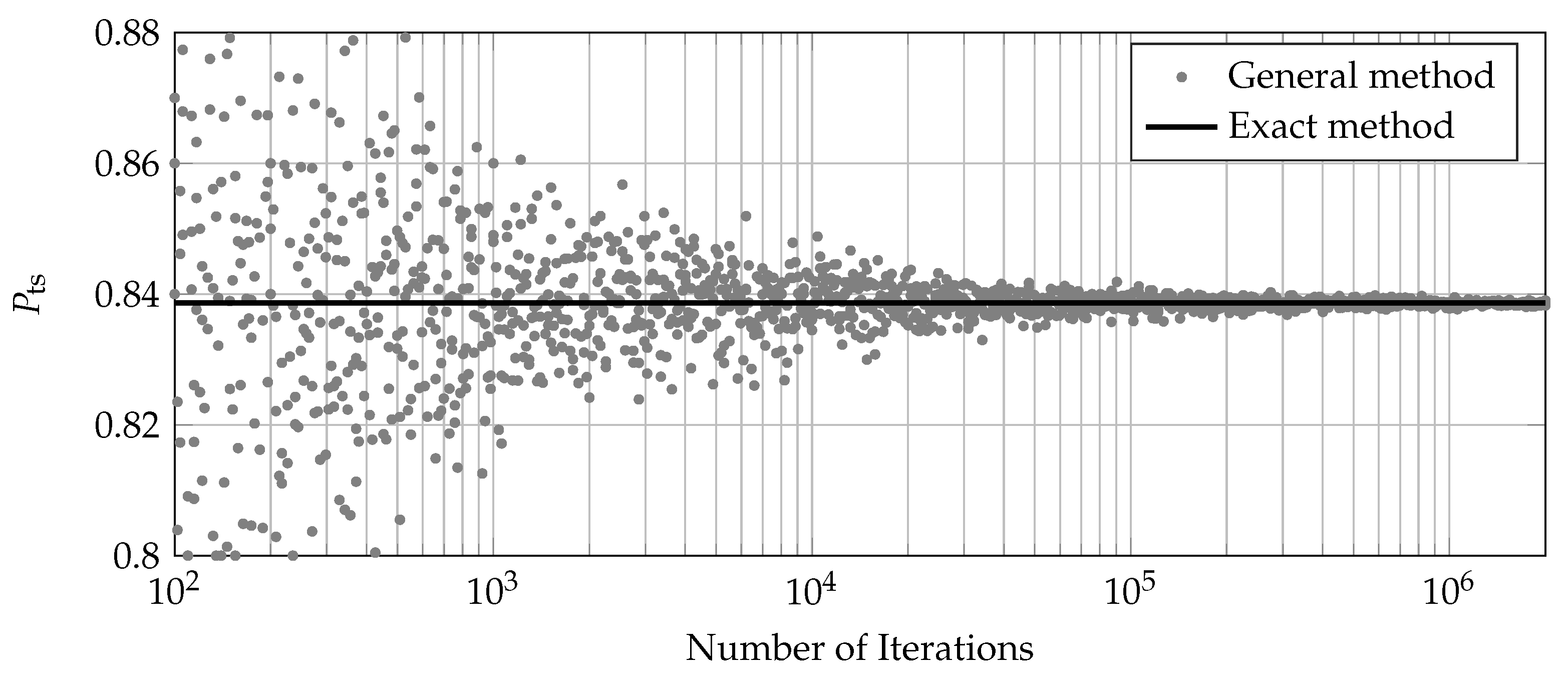
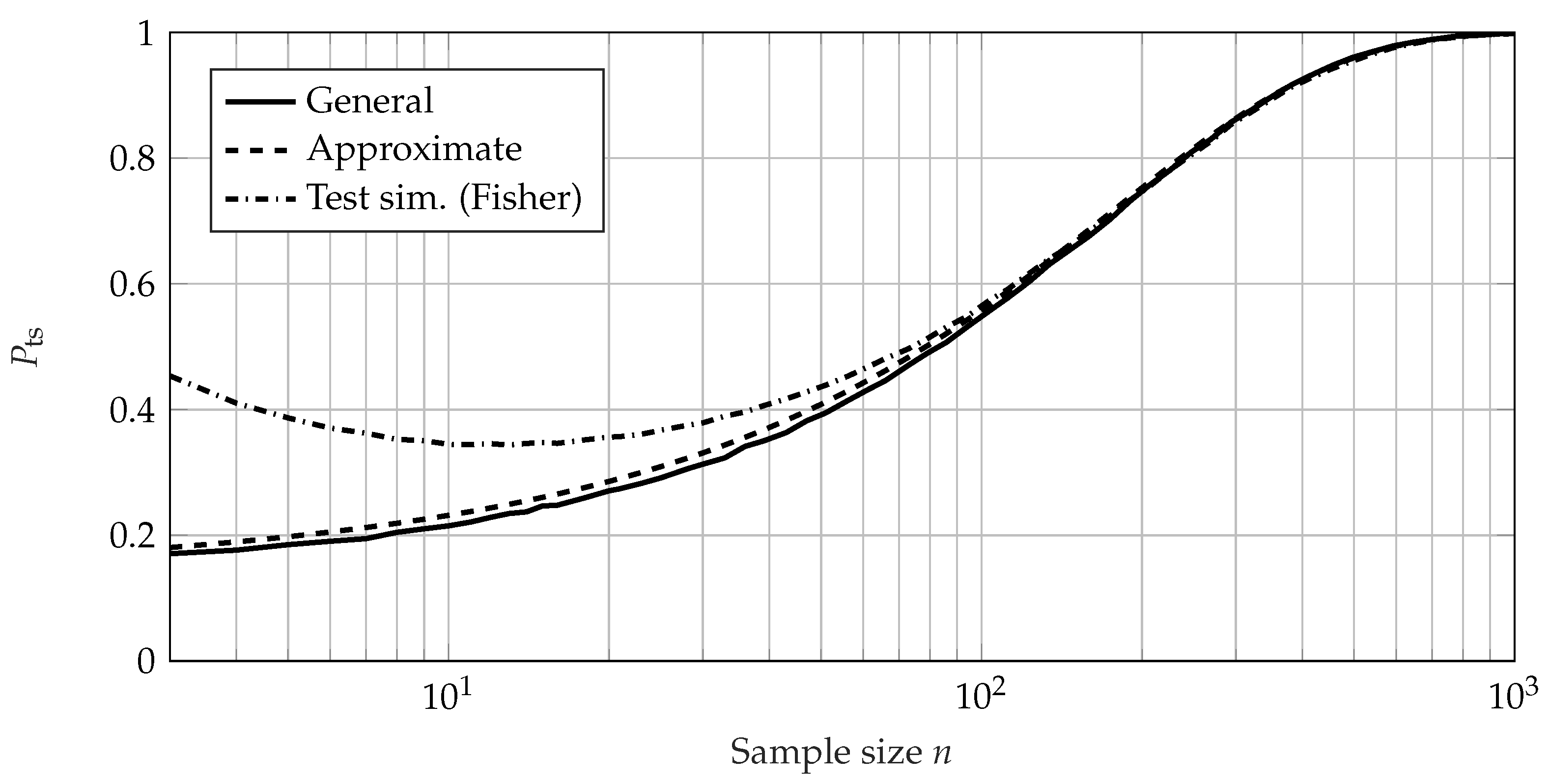
3.4. Calculation by Test Simulation

To ensure proper reflection of the large possible number of correlations and effects in a test that is actually carried out and evaluated following test planning, it is possible to use those methods for test evaluation and calculation of confidence bounds which are used in the actual test. For this purpose, the hypothesis-testing concepts can be left aside in favor of the MCS approach of Dazer et al. [45,46,61], which relies solely on the law of large numbers. The procedure is as follows: draw pseudo-random failure times to generate samples according to the sample behavior of the test and prior knowledge; estimate the failure distribution and confidence level using this sample along with the methods which are actually used later on; and check whether the requirement is met. By iterating multiple times, P ts can be calculated via [46]
P ts = Number   of   successful   simulsted   tests Total   number   of   simulsted   tests .
The idea is to use the methods of test evaluation which are used on the actual test later on. No constructs or alterations for a hypothesis-testing approach are needed. The very popular Fisher and likelihood ratio confidence bounds [8,10] can be used here. However, there may be drawbacks in terms of accuracy due to a high number of MCS iterations and possible estimation bias amplification.

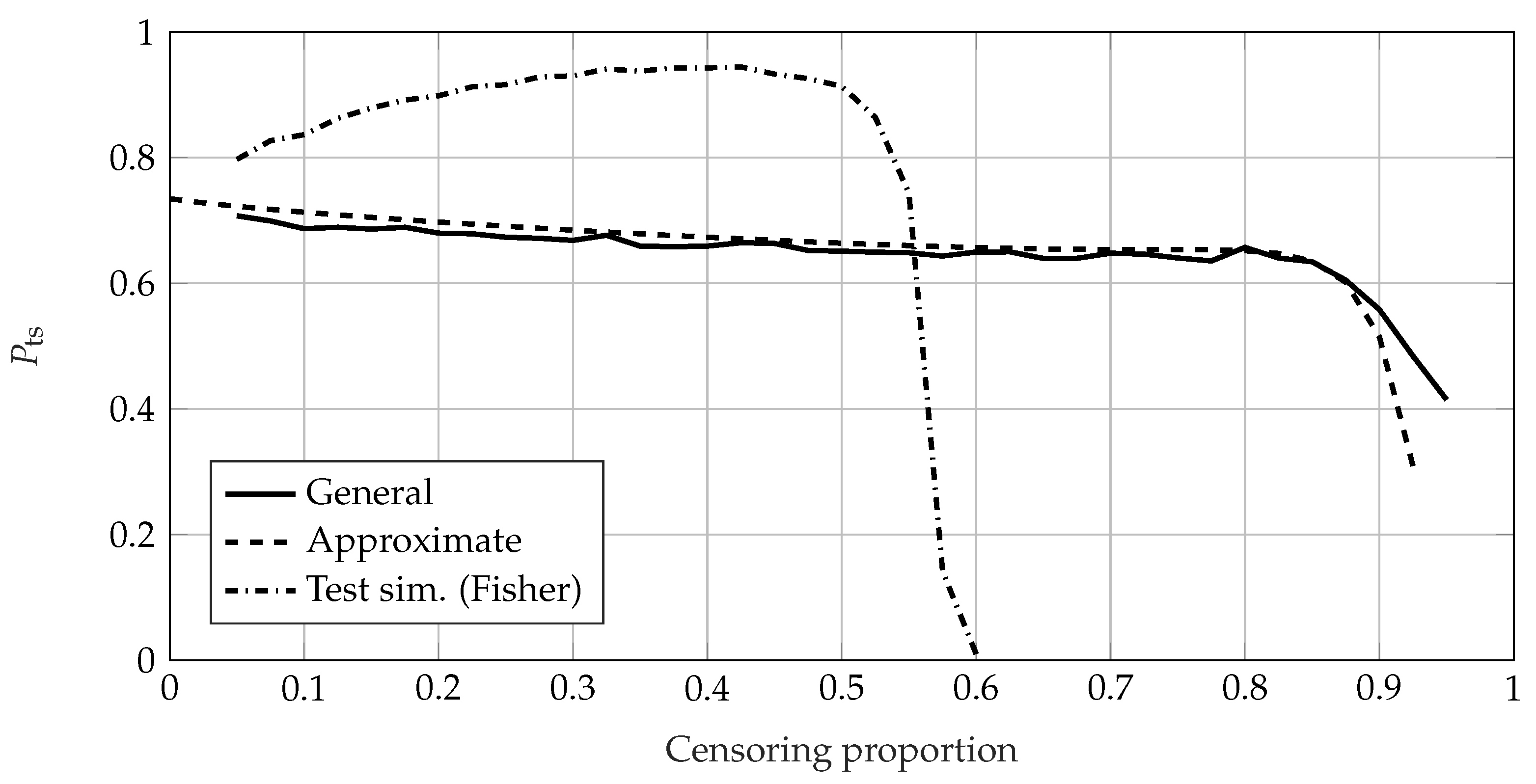
4. Comparison of the Calculation Methods for the Probability of Test Success

The presented methods for calculating P ts perform differently, and they can each be beneficial in different scenarios. In order to compare them and work out the differences, several values of P ts are calculated. However, a comprehensive and holistic view can only be obtained through an extensive parameter study, which is not the focus here. The methods are compared using the SR test, as well as the uncensored and censored EoL test.

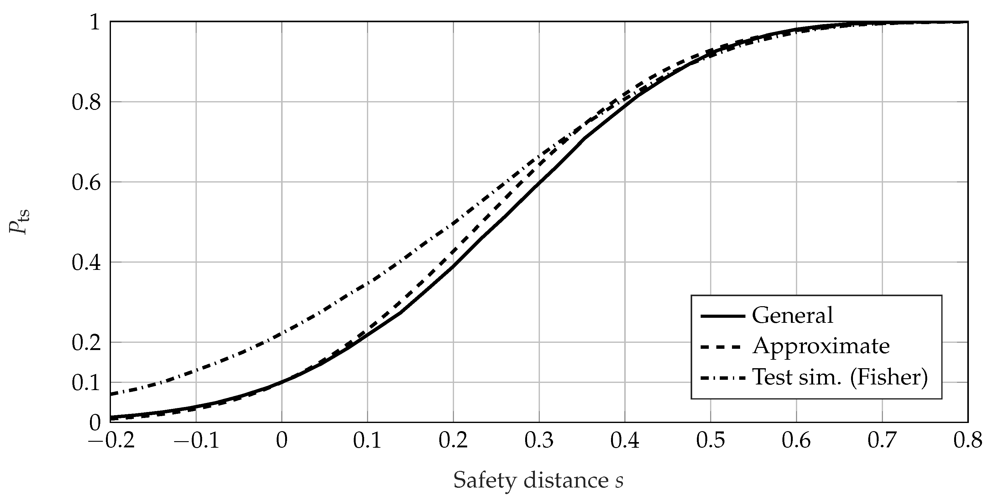
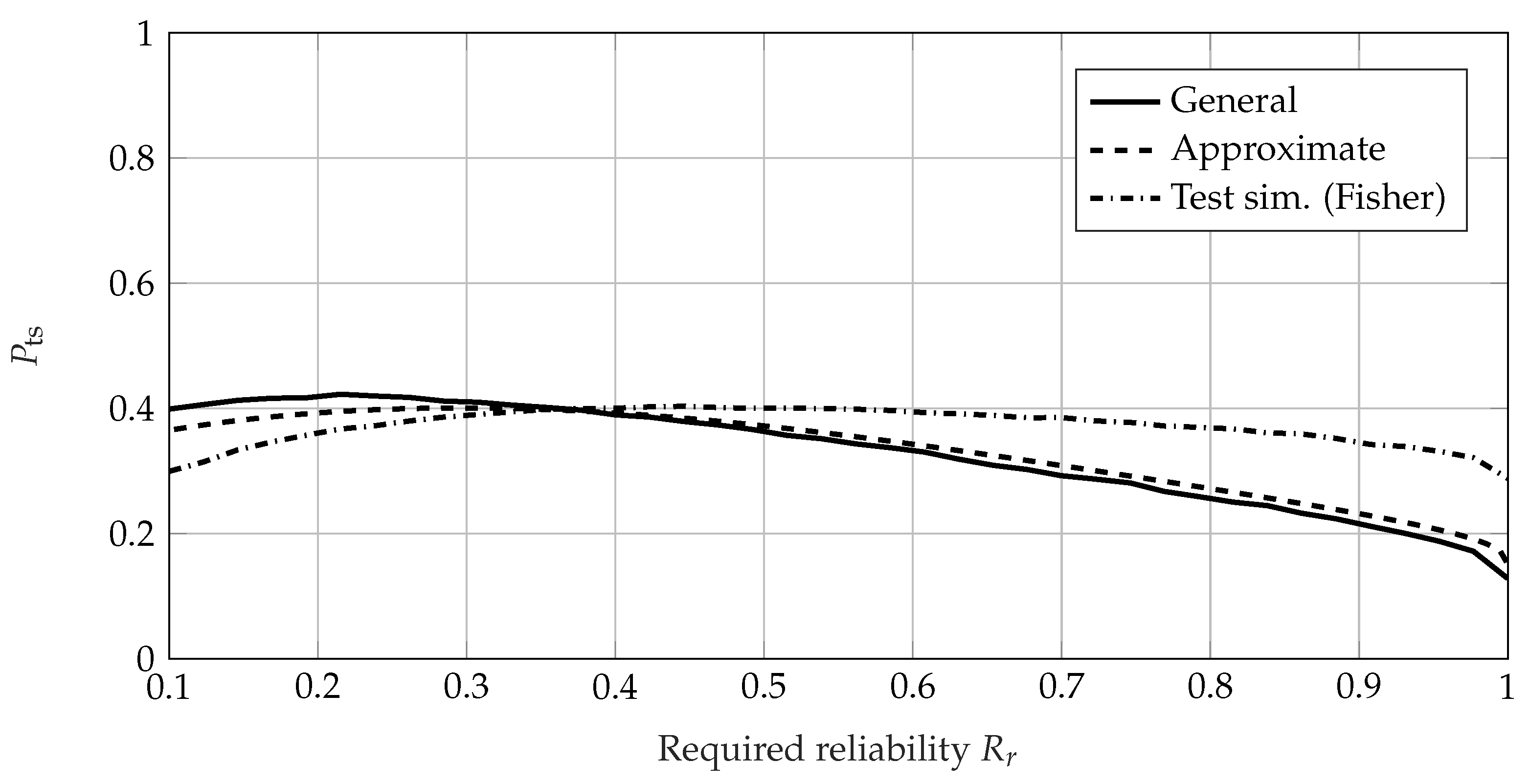
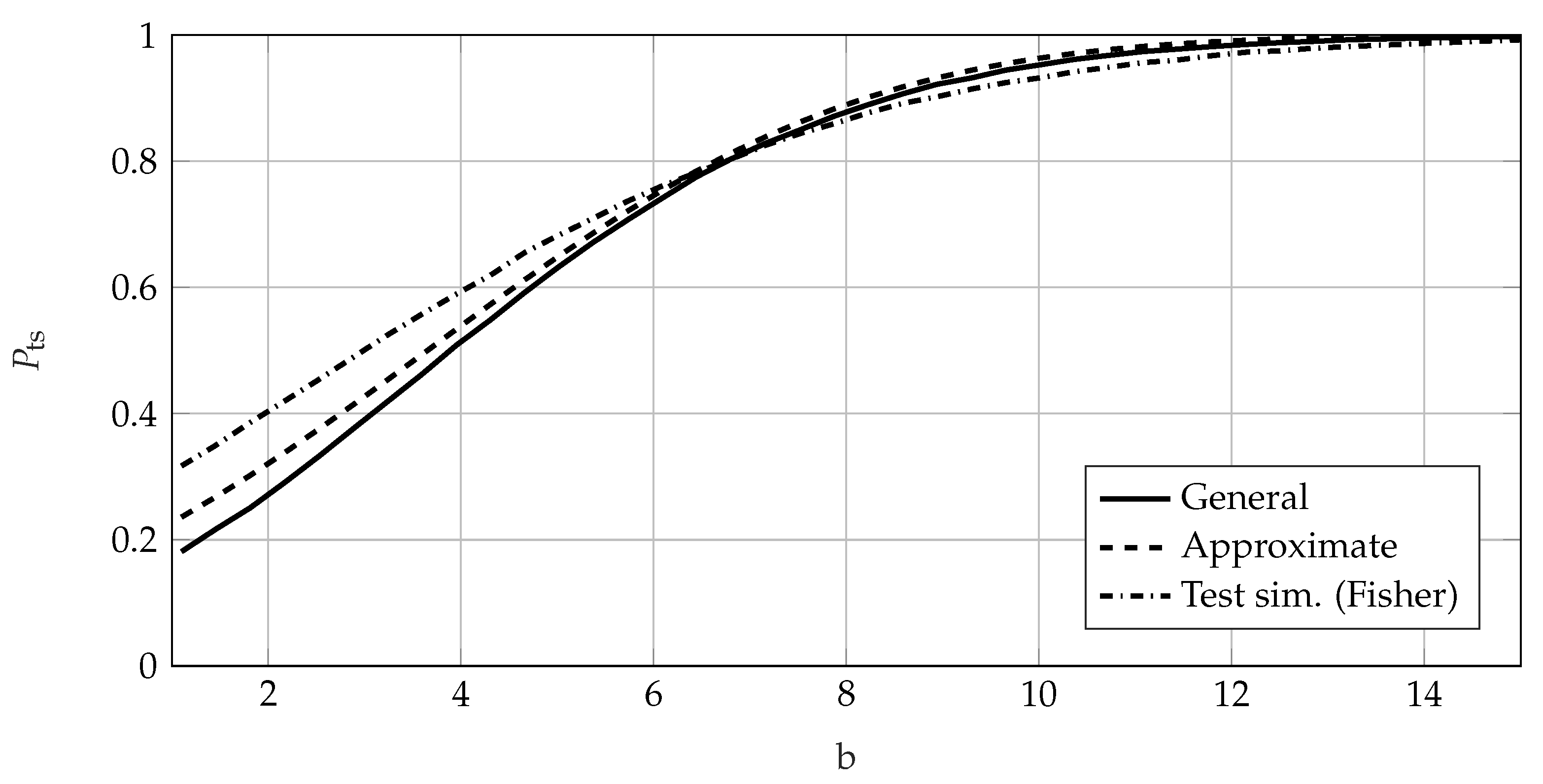
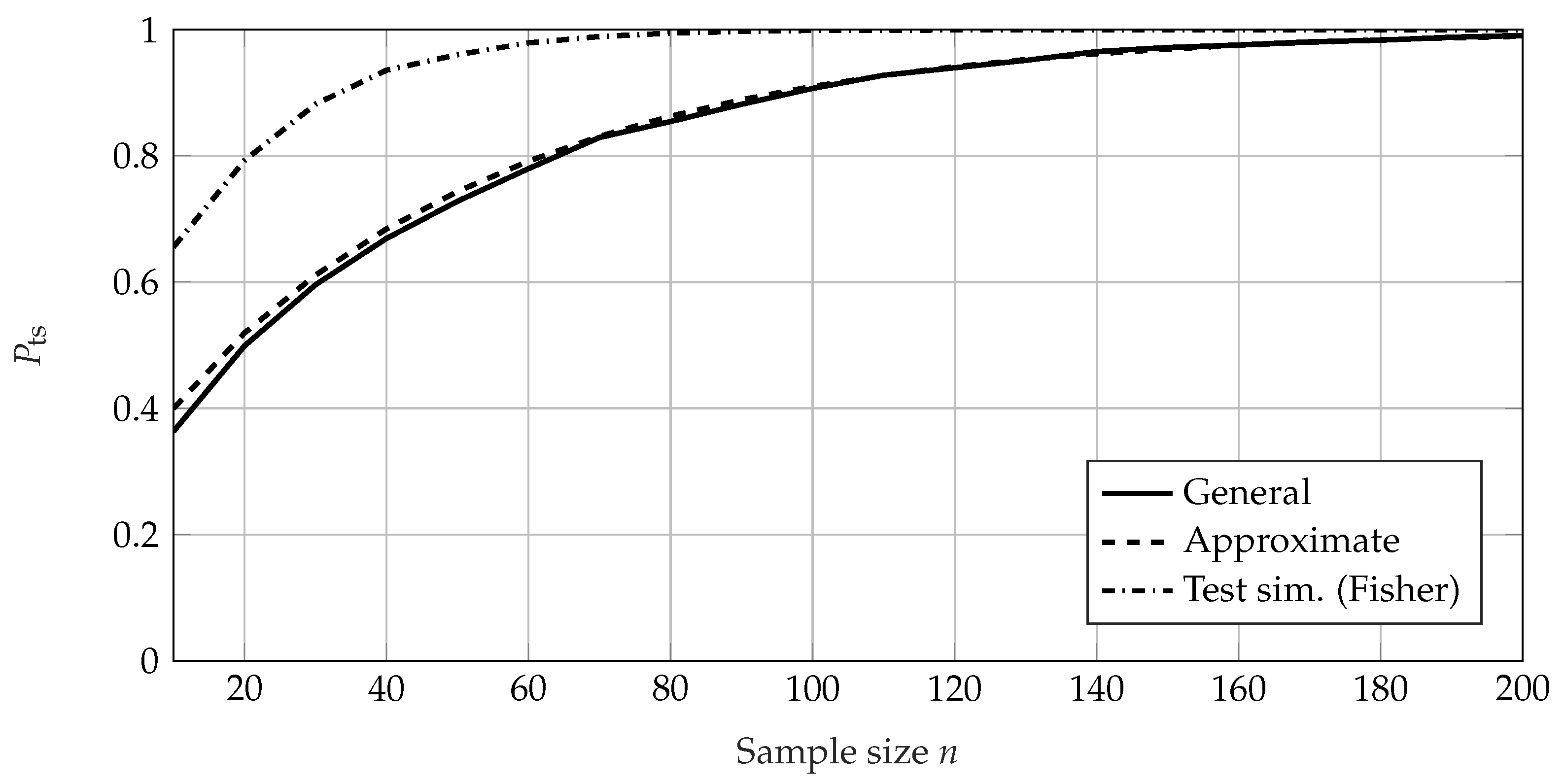
4.1. Comparison Using Success Run Tests

For calculating the P ts of an SR test, the general method, the exact method, and the test simulation method can be used. Due to the lack of an MLE and confidence level estimation, the general calculation method coincides with the method of test simulation. As no MLE takes place during the SR test, no influence of an estimation method is expected and the general method converges to the exact method. This can be seen in Figure 4 for a requirement of R r = C r = 90 % .
The MCS of the general method converges to the exact method; 100,000 iterations ensures reasonable accuracy in this scenario with the prior knowledge as Weibull-distributed failures, with b = 3 and T = 1 and no allowed failures for the lifetime requirement of t r = 0.2 ( s = 0.577 ). When scenarios using different prior knowledge and different requirements are analyzed, and when failures are allowed, similar behavior is shown, leading to the conclusion that the exact method is to be preferred for calculating the P ts of an SR test. In addition, the exact method is much more effortless to use, as no MCS iteration has to take place.

4.2. Comparison Using Failure-Based Tests

For EoL tests, the following methods are used to calculate P ts :
  • General method (General);
  • Approximate method (Approximate);
  • Test simulation method (Test sim.).
In Figure 5, P ts is calculated using the approximate method as well as the general method for a parameter-free sample quantile estimation (sample q.) and a quantile estimation via distribution estimation using MLE.
It can be seen that the general method and the approximate method (see (27)) show very good agreement if parameter-free quantile estimation is used. On the other hand, the approximation based on the MLE (see (41)) shows very good agreement with the general method if the MLE is used for quantile estimation. Therefore, the approximation solely based on the sample quantiles (27) is to be used if empirical sample quantile estimation is used in the test. If the very common MLE is used for distribution parameter and quantile estimation, the approximate approach in (41) should be used instead of (27). The offset between the P ts of the sample quantile estimation and the MLE is due to the nature of the estimation method. The MLE uses the information of all failure times, whereas the sample quantile estimation primarily uses information about the number of failures. In Figure 6, Figure 7, Figure 8, Figure 9 and Figure 10, the P ts of the general method, the approximate method, and the test simulation method is shown for the variables n, s, R r , C r , and b, respectively. Because MLE is used, Equation (41) is used for the approximate method. For each calculation, 100,000 iterations were performed for the bootstrap of the general method and the MCS of the test simulation method.
The approximate method shows a very good fit to the values of the general calculation method. However, the test simulation method using a Fisher confidence bound shows a significant offset in respect of the other methods. In particular, with sample size n (see Figure 6), an increase in P ts with smaller sample sizes for n < 20 can be seen. This is due to the enhanced effect of the MLE bias, which causes the estimates of the Weibull parameters to be noticeably biased in small samples [45]. However, for very large sample sizes the test simulation method shows identical values of P ts compared to the general method for n > 100 . This seems to be a large enough sample size to remedy the bias. Additionally, these matching values verify the approach following the hypothesis testing framework and its calculation according to the general method and the approximate method. Looking at the values of P ts with regard to the safety distance s in Figure 7, a similar behavior can be seen. The general method shows conformity with the test simulation method for large safety distances ( s > 0.4 ) and the approximate calculation shows a good fit. For a safety distance of s = 0 , which means the effect size equals zero ( Δ = 0 ), the statistical power of a test is the complement of the chosen confidence level. This translates to a value of P ts equaling the complement of the required confidence, namely, P ts = 1 C r for s = 0 . This can be seen in Figure 1 and (6) and (7), with both distributions f H 0 and f H 1 being the same. Both the approximate method and the general method show this behavior and yield values of P ts = 10 % for s = 0 , as C r = 90 % in Figure 7. Therefore, they are verified in this regard. However, the test simulation method shows an offset, which is presumably again due to the amplified bias of this method. The approximate method shows good conformity with the general method with regard to the required reliability R r ; see Figure 8. The test simulation method shows different behavior, with a nearly constant P ts . In Figure 9, the values of P ts are shown with respect to the required confidence level C r . Similar to the behavior seen in Figure 8, the approximate method shows very good agreement with the general method and the test simulation method shows a small offset. In Figure 10, the approximate method shows good agreement with the P ts values of the general method with regard to the Weibull shape parameter b of the prior knowledge. The test simulation method again shows a significant offset.
For a censored EoL test, the approximate method remains a very good approximation. Figure 11 shows P ts with regard to sample size of the different methods for moderate right-censoring of 30 % of the specimen. Although the test simulation method shows a very similar curve of P ts , the values are much higher than the ones of the general and approximate methods. Figure 12 shows the P ts of the methods with regard to the censoring proportion for a sample size of n = 40 .
The test simulation method shows a significant offset in censored EoL tests compared to the general method. The approximate method shows very good conformity for almost all censoring proportions here.

4.3. Conclusion of the Comparison
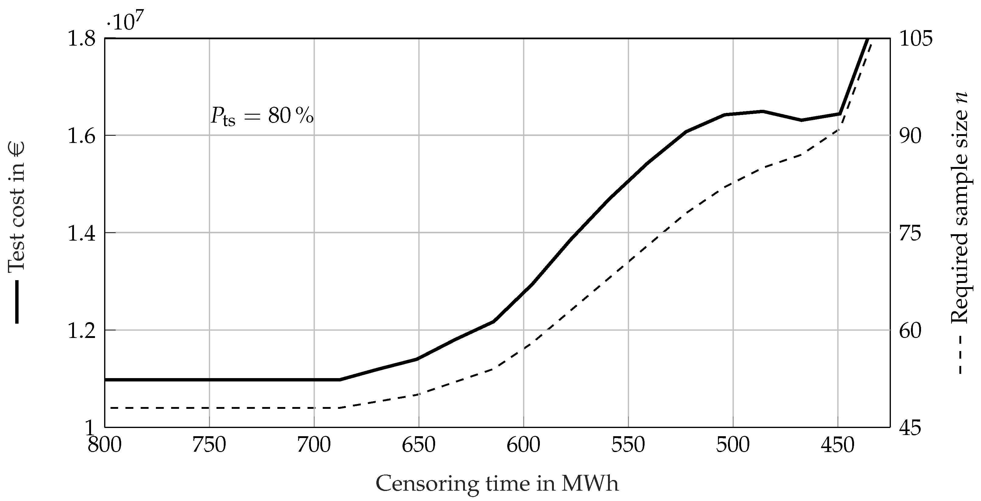
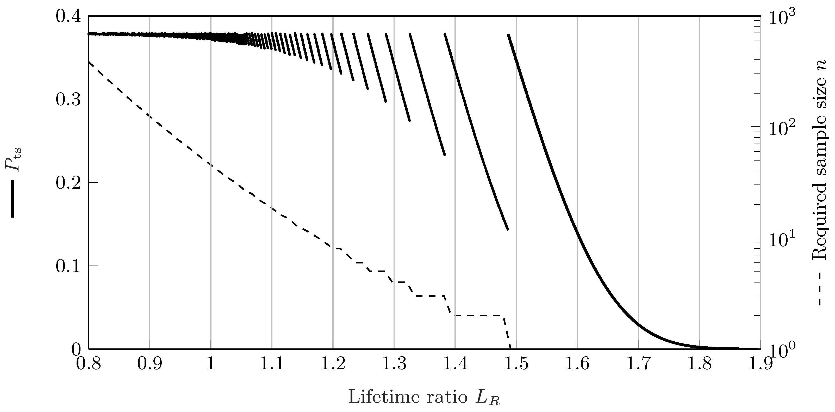
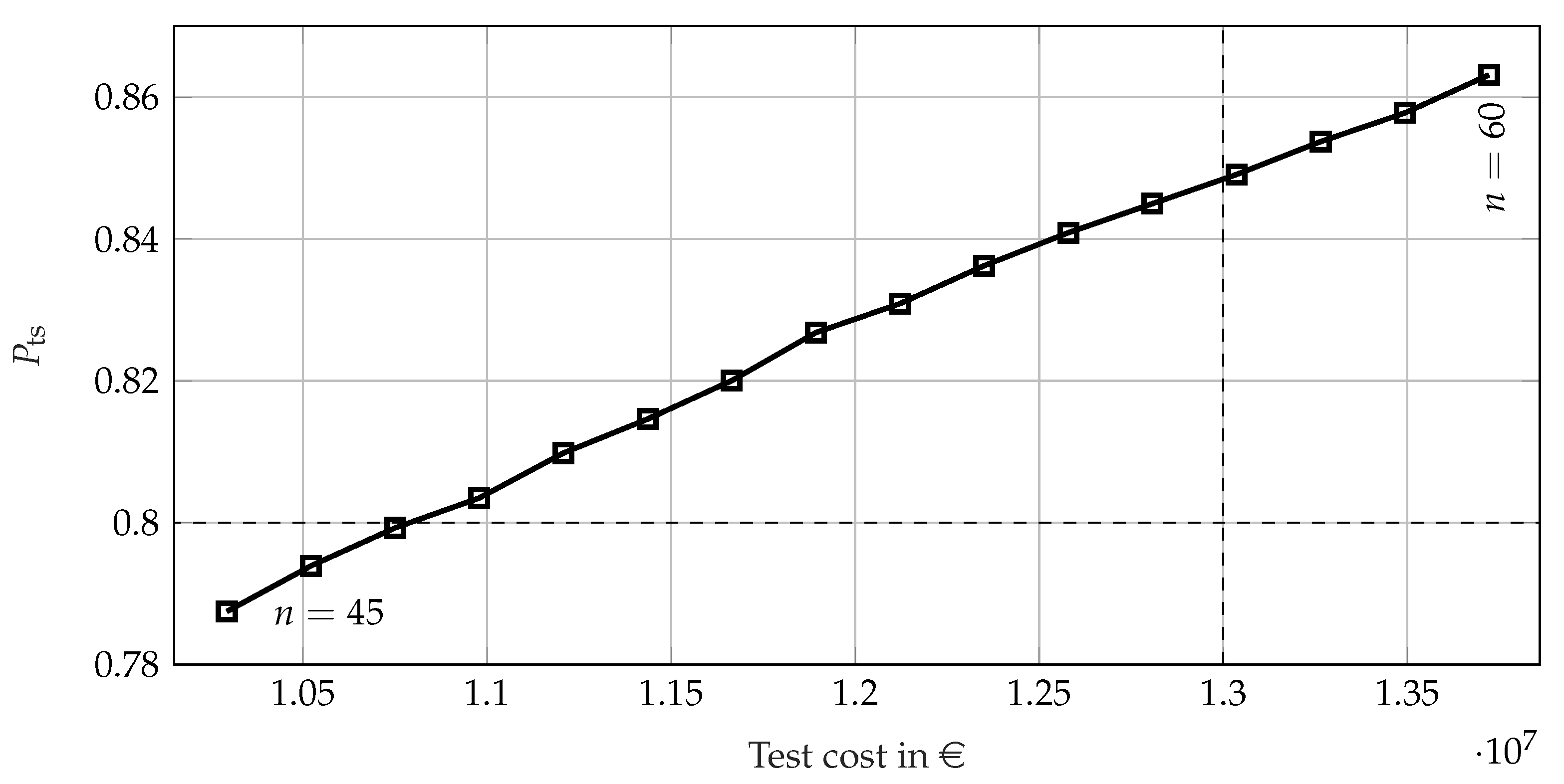
From these comparisons, it can be concluded that the approximate calculation is a good fit for most applications. If a precise calculation is desired, the general method should be used, as the accuracy can be set as desired via the number of iterations. The approximate method can be used for MLE and sample quantile estimation approximation. Both seem to approximate very well, even for smaller sample sizes. The calculation using the test simulation is plagued by the same disadvantages as the physical test evaluation methods. Therefore, it should be investigated if a bias correction is of use in the individual case. The values of P ts of censored EoL tests are best calculated using the general method. However, even the approximate calculation shows very good results. The calculation methods for the SR test shows a very strong advantage when using the exact method instead of the general method. Consequently, the exact method should always be used where an SR test is concerned. For SR tests, the general method and the test simulation method coincide due to the lack of quantile estimation. These findings are summarized in Table 2.

5. Case Study

The Probability of Test Success, P ts , enables objective assessment of different test types and scenarios. In addition, it allows the reliability engineer to identify feasible regions of test designs and enables an optimal test for reliability demonstration. In order to demonstrate these benefits, a reliability demonstration test for a high-voltage battery of a battery–electric vehicle is planned and explained here. The lifetime of the battery is the accumulated energy throughput (ETP) for which a reliability requirement of R r = 95 % , C r = 90 % and t r = 400 MWh is to be demonstrated. Because of the battery technology and use case being a very recent development, no usable tests of prior product generations can be used as prior knowledge. However, during research and development a simulation model was established for the prediction of the ETP using the driving profiles of several measurements in the field. Therefore, the simulation was able to yield an estimation of the lifetime of the battery. The exemplary simulation results are taken from [62]. Using the simulation model and a failure criterion of 80 % state of health, the Weibull distributed failure behavior of the battery can be found. The parameters are T = 596.37 MWh and b = 9.598 (see Table 3). This failure distribution can be then used as prior knowledge for the reliability demonstration test planning of the battery.
As a first step, the feasible region of test design is analyzed using the exact method of the SR test as well as the approximate method for the EoL test. Because an MLE has to be used for test evaluation, the MLE is used for both the approximate method and the general method. The P ts for the uncensored EoL test with regard to the sample size n is shown in Figure 13.
For an adequate value of P ts = 80 % of the EoL test, a specimen n 50 should be used. The values of P ts in the right-censored EoL test for several sample sizes and censoring proportions can be seen in Figure 14.
A greater censoring proportion requires a larger sample size in order to reach a value of P ts 80 % . For a moderate censoring proportion of 10 % , the required sample size is >50, and for a censoring proportion of about 50 % , the required sample size is >70. In order to assess the benefit of censoring as well as the costs one test would generate, the median of the total test costs can be calculated approximately using (36) and the sample size. For demonstration purposes, we assume the cost of one specimen as EUR 2,000 and the cost of testing one specimen as 400 EUR/MWh. The median of the total test costs of the uncensored EoL test calculated using the approximation can be seen in Figure 13. The total test costs and the required sample size of the censored EoL test for a value of P ts = 80 % are shown in Figure 15 (type II censoring) and Figure 16 (type I censoring).
The censoring enables a maximum reduction in costs of about 21 % for a fixed sample size. However, stronger censoring results in lower values of P ts , which in turn result in a higher required sample size, and thus higher test costs. The SR test without permitted failures and no lifetime ratio does need n = 45 specimen to survive t r = 400 MWh in order to demonstrate the requirement of Table 3 (using (15)). However, when using (16), the SR test only yields a value of P ts = 37.8 % ; therefore, it should not be used at all. The values of P ts in an SR test using a lifetime ratio can be seen in Figure 17.
The required sample size for SR tests using the lifetime ratio is calculated accordingly, using (19) and (20). It can be seen that the SR test using a lifetime ratio reaches its maximum value of P ts at 37.8 % . The required sample size increases exponentially for decreasing values of L r and quickly drops to 1 for L R > 1 due to the large shape parameter of the Weibull distribution.
Using the information of the approximate calculations shown in Figure 13, Figure 14, Figure 15 and Figure 16, the feasible region for a value of P ts = 80 % for the EoL test in this scenario is a sample size between n 45 and n 60 . Therefore, the P ts of the uncensored EoL test is calculated using the general method for sample sizes between 45 and 60. Censoring the EoL test does not yield benefits here, as the cost of achieving the desired value of P ts = 80 % increases with the increase in the censoring proportions; see Figure 15 and Figure 16. A budget of EUR 13 million is available for reliability demonstration; therefore, the test needs to be assessed in terms of costs. The distribution of the costs can be calculated using the generated failure times of the bootstrap approach in the general method. Therefore, the P ts of the EoL test can be shown with regard to the test costs; see Figure 18.
It can be seen that a sample size of n = 48 has P ts = 80.35 % and costs EUR 10.98 million for the uncensored EoL test. Therefore, it is the most efficient test in terms of reliability demonstration. Alternatively, in order to use the whole budget, an EoL test using n = 56 samples yields an even greater value of P ts = 84.5 % , while costing EUR 12.81 million. Due to the high value of the Weibull shape parameter of b = 9.6 , the total test costs do not scatter to a great extent for the uncensored EoL test with a standard deviation of σ = EUR 195,000 ( n = 48 ) and σ = EUR 215,000 ( n = 56 ). Here, the SR test is unsuitable due to a value of P ts < 50 % , however, it costs significantly less than the EoL tests, with a total test cost of EUR 7.29 million. Only through objective assessment using the P ts can the risk of a failing test be acounted for in the decision-making process of reliability test planning. In 62 % of cases, the EUR 7.29 million of the SR test would not suffice for reliability demonstration, as failures would occur during testing.

6. Discussion and Conclusions

The estimation of the success rate of a reliability test is established and defined herein as the Probability of Test Success. This enables consideration of the type II error in reliability test planning and represents the statistical power held by a reliability test. Therefore, it is an indispensable metric and tool for the planning of efficient reliability demonstration tests. In addition to the general calculation method, which uses a bootstrap approach and allows all reliability tests to be assessed, an approximate method is introduced. It enables a fast and easy to implement calculation of most reliability demonstration tests, such as uncensored and censored EoL, tests without the need for a Monte Carlo simulation. The exact method for calculating the P ts of an SR test is the best method in all SR test planning scenarios. In addition, a method for calculating P ts by test simulation is shown. The comparison shows very good performance for both the general and approximate methods. However, the performance of the test simulation method is subject to the flaws of the estimation methods being used, and often does not agree with the general and the approximate methods for small sample sizes. A case study demonstrates the use and benefits for the planning process as well as the possibilities in terms of monetary decision making in reliability demonstration test planning. The approximate method enables the identification of the feasible test design region, while the general method allows precise calculation and assessment in terms of the cost of the tests to be performed. It has been shown that an objective assessment of reliability tests using the P ts is required for balanced decision-making in reliability test planning. In principle, the approach can be applied to all technical products. For example, in the case of structural mechanical failure of brake calipers, chassis structures, and electronic components such as inverters as well as vehicles, aircraft, ships, cable cars, elevators, rail vehicles, combustion engines, and much more. Additional research could enable the concept for accelerated tests as well as test planning for systems with multiple failure modes. The approach of using the MLE for the approximate calculation as well as for the general calculation can be easily adapted to incorporate additional parameters of a lifetime model for accelerated tests. Furthermore, the uncertainty of the prior knowledge can be implemented into the concept in order to account for uncertain prior knowledge, thereby ensuring more accurate estimates of the P ts .

Author Contributions

Conceptualization, A.G. and M.D.; methodology, A.G.; software, A.G.; validation, A.G., T.H. and M.D.; formal analysis, A.G. and M.D.; investigation, A.G.; resources, A.G.; data curation, A.G.; writing—original draft preparation, A.G.; writing—review and editing, A.G. and M.D.; visualization, A.G.; supervision, A.G. and M.D.; project administration, A.G. All authors have read and agreed to the published version of the manuscript.

Funding

This research received no external funding.

Institutional Review Board Statement

Not applicable.

Data Availability Statement

Not applicable.

Conflicts of Interest

The authors declare no conflict of interest.

Abbreviations

The following abbreviations are used in this manuscript:
DOEDesign of experiments
SRSuccess run
SDSudden death
MCSMonte Carlo simulation
MTTFMean time to failure
EoLEnd of life
MLEMaximum likelihood estimation
CLTCentral limit theorem
ETPAccumulated energy throughput
pdfProbability density function
cdfCumulative distribution function
pmfProbability mass function

References

  1. Montgomery, D.C. Design and Analysis of Experiments, 10th ed.; John Wiley & Sons: Hoboken, NJ, USA, 2020. [Google Scholar]
  2. Siebertz, K.; van Bebber, D.; Hochkirchen, T. Statistische Versuchsplanung; Springer: Berlin/Heidelberg, Germany, 2010. [Google Scholar] [CrossRef]
  3. McPherson, K. On choosing the number of interim analyses in clinical trials. Stat. Med. 1982, 1, 25–36. [Google Scholar] [CrossRef]
  4. Choi, S.C.; Smith, P.J.; Becker, D.P. Early Decision in Clinical Trials When the Treatment Differences Are Small. Experience of a Controlled Trial in Head Trauma. Control. Clin. Trials 1985, 6, 280–288. [Google Scholar] [CrossRef]
  5. Trzaskoma, B.; Sashegyi, A. Predictive Probability of Success and the Assessment of Futility in Large Outcomes Trials. J. Biopharm. Stat. 2007, 17, 45–63. [Google Scholar] [CrossRef]
  6. Rufibach, K.; Burger, H.U.; Abt, M. Bayesian predictive power: Choice of prior and some recommendations for its use as probability of success in drug development. Pharm. Stat. 2016, 15, 438–446. [Google Scholar] [CrossRef] [PubMed]
  7. Squeglia, N.L. Zero Acceptance Number Sampling Plans, 5th ed.; ASQ Quality Press: Milwaukee, WI, USA, 2008. [Google Scholar] [CrossRef]
  8. Meeker, W.Q.; Escobar, L.A. Statistical Methods for Reliabillity Data; John Wiley & Sons: New York, NY, USA; Chichester, UK; Weinheim, Germany; Brisbane, Australia; Singapore; Toronto, ON, Canada, 1998; p. 680. [Google Scholar]
  9. Nelson, W.B. Applied Life Data Analysis; John Wiley & Sons: Hoboken, NJ, USA, 2004. [Google Scholar]
  10. Bertsche, B. Reliability in Automotive and Mechanical Engineering; Springer: Berlin, Germany, 2008. [Google Scholar] [CrossRef]
  11. Bayes, M.; Price, M. An Essay Towards Solving a Problem in the Doctrine of Chances. By the Late Rev. Mr. Bayes, F. R. S. Communicated by Mr. Price, in a Letter to John Canton, AMFR S. Philos. Trans. R. Soc. Lond. 1763, 53, 370–418. [Google Scholar] [CrossRef]
  12. Beyer, R.; Lauster, E. Statistische Lebensdauerprüfpläne bei Berücksichtigung von Vorkenntnissen. Qualität und Zuverlässigkeit 1990, 35, 93–98. [Google Scholar]
  13. Grundler, A.; Bartholdt, M.; Bertsche, B. Statistical test planning using prior knowledge—Advancing the approach of Beyer and Lauster. In Proceedings of the Safety and Reliability—Safe Societies in a Changing World, Trondheim, Norway, 17–21 June 2018; pp. 809–814. [Google Scholar] [CrossRef]
  14. Guida, M.; Pulcini, G. Automotive reliability inference based on past data and technical knowledge. Reliab. Eng. Syst. Saf. 2002, 76, 129–137. [Google Scholar] [CrossRef]
  15. Kleyner, A.; Bhagath, S.; Gasparini, M.; Robinson, J.; Bender, M. Bayesian techniques to reduce the sample size in automotive electronics attribute testing. Microelectron. Reliab. 1997, 37, 879–883. [Google Scholar] [CrossRef]
  16. Kleyner, A.; Elmore, D.; Boukai, B. A Bayesian Approach to Determine Test Sample Size Requirements for Reliability Demonstration Retesting after Product Design Change. Qual. Eng. 2015, 27, 289–295. [Google Scholar] [CrossRef]
  17. Krolo, A.; Rzepka, B.; Bertsche, B. Application of Bayes statistics to reduce sample-size, considering a lifetime-ratio. In Proceedings of the Annual Reliability and Maintainability Symposium, Seattle, WA, USA, 28–31 January 2002; pp. 577–583. [Google Scholar] [CrossRef]
  18. Krolo, A.; Rzepka, B.; Bertsche, B. The Use of the Bayes Theorem to Accelerated Life Tests. In Proceedings of the European Conference on Safety and Reliability ESREL, Lyon, France, 18–21 March 2002. [Google Scholar]
  19. Krolo, A. Planung von Zuverlässigkeitstests mit Weitreichender Berücksichtigung von Vorkenntnissen. Ph.D. Thesis, University of Stuttgart, Stuttgart, Germany, 2004. [Google Scholar]
  20. Savchuk, V.P.; Martz, H.F. Bayes Reliability Estimation Using Multiple Sources of Prior Information: Binomial Sampling. IEEE Trans. Reliab. 1994, 43, 138–144. [Google Scholar] [CrossRef]
  21. Grundler, A.; Bollmann, M.; Obermayr, M.; Bertsche, B. Berücksichtigung von Lebensdauerberechnungen als Vorkenntnis im Zuverlässigkeitsnachweis. In Proceedings of the VDI-Fachtagung Technische Zuverlässigkeit 2019, Mannheim, Germany, 2–3 July 2019. [Google Scholar]
  22. Genest, C.; Zidek, J.V. Combining Probability Distributions: A Critique and an Annotated Bibliography. Stat. Sci. 1986, 1, 114–148. [Google Scholar]
  23. Hitziger, T.; Bertsche, B. An approach to determine uncertainties of prior information—The transformation factor. In Proceedings of the European Conference on Safety and Reliability ESREL, Tri City, Poland, 27–30 June 2005; Volume 1, pp. 843–849. [Google Scholar]
  24. Lu, L.; Li, M.; Anderson-Cook, C.M. Multiple objective optimization in reliability demonstration tests. J. Qual. Technol. 2016, 48, 326–342. [Google Scholar] [CrossRef]
  25. Hamada, M.S.; Wilson, A.G.; Reese, C.S.; Martz, H.F. Bayesian Reliability; Springer: New York, NY, USA, 2008. [Google Scholar] [CrossRef] [Green Version]
  26. Lindley, D.V.; Singpurwalla, N.D. Adversarial Life Testing. J. R. Stat. Soc. Ser. B (Methodol.) 1993, 55, 837–847. [Google Scholar] [CrossRef]
  27. Wilson, K.J.; Farrow, M. Assurance for Sample Size Determination in Reliability Demonstration Testing. Technometrics 2021, 63, 523–535. [Google Scholar] [CrossRef]
  28. Guo, H.; Pohl, E.; Gerokostopoulos, A. Determining the Right Sample Size for Your Test: Theory and Application. In Proceedings of the 2013 Annual Reliability and Maintainability Symposium, Orlando, FL, USA, 28–31 January 2013. [Google Scholar]
  29. Arizono, I.; Kawamura, Y.; Takemoto, Y. Reliability tests for Weibull distribution with variational shape parameter based on sudden death lifetime data. Eur. J. Oper. Res. 2008, 189, 570–574. [Google Scholar] [CrossRef]
  30. Huang, S.R.; Wu, S.J. Reliability sampling plans under progressive type-I interval censoring using cost functions. IEEE Trans. Reliab. 2008, 57, 445–451. [Google Scholar] [CrossRef]
  31. Vlcek, B.L.; Hendricks, R.C.; Zaretsky, E.V. Monte Carlo simulation of sudden death bearing testing. Tribol. Trans. 2004, 47, 188–199. [Google Scholar] [CrossRef] [Green Version]
  32. Hsieh, H.K. Average Type-II Censoring Times for the 2-Parameter Weibull Distribution. IEEE Trans. Reliab. 1994, 43, 91–96. [Google Scholar] [CrossRef]
  33. Tsai, T.R.; Lu, Y.T.; Wu, S.J. Reliability sampling plans for Weibull distribution with limited capacity of test facility. Comput. Ind. Eng. 2008, 55, 721–728. [Google Scholar] [CrossRef]
  34. Kirchner, E. Werkzeuge und Methoden der Produktentwicklung: Von der Idee zum Erfolgreichen Produkt; Springer: Berlin, Germany, 2020. [Google Scholar]
  35. Cohen, J. Statistical Power Analysis for the Behavioral Sciences, 2nd ed.; Lawrence Erlbaum Associates: New York, NY, USA, 1988. [Google Scholar]
  36. Neyman, J.; Pearson, E.S. On the Use and Interpretation of Certain Test Criteria for Purposes of Statistical Inference: Part I. Biometrika 1928, 20A, 175–240. [Google Scholar]
  37. Neyman, J.; Pearson, E.S., IX. On the problem of the most efficient tests of statistical hypotheses. Philos. Trans. R. Soc. A Math. Phys. Eng. Sci. 1933, 231, 289–337. [Google Scholar] [CrossRef] [Green Version]
  38. Grundler, A.; Dazer, M.; Bertsche, B. Reliability-Test Planning Considering Multiple Failure Mechanisms and System Levels. In Proceedings of the Annual Reliability and Maintainability Symposium, Palm Springs, CA, USA, 27–30 January 2020. [Google Scholar]
  39. Grundler, A.; Dazer, M.; Herzig, T.; Bertsche, B. Considering Multiple Failure Mechanisms in Optimal Test Design. In Proceedings of the Proceedings IRF2020: 7th International Conference Integrity-Reliability-Failure, Funchal, Portugal, 6–10 September 2020; pp. 673–682. [Google Scholar]
  40. Grundler, A.; Dazer, M.; Bertsche, B. Effect of Uncertainty in Prior Kowledge on Test Planning for a Brake Caliper using the Probability of Test Success. In Proceedings of the Proceedings—Annual Reliability and Maintainability Symposium, Orlando, FL, USA, 24–27 May 2021. [Google Scholar]
  41. Grundler, A.; Dazer, M.; Herzig, T.; Bertsche, B. Efficient System Reliability Demonstration Tests Using the Probability of Test Success. In Proceedings of the Proceedings of the 31st European Safety and Reliability Conference ESREL 2021, Angers, France, 19–23 September 2021; pp. 1654–1661. [Google Scholar] [CrossRef]
  42. MIL-STD-1916; Department of Defense Test Method Standard; Department of Defense: Washington, DC, USA, 1996.
  43. John, P.W.M. Statistical Methods in Engineering and Quality Assurance; Chapman and Hall/CRC: London, UK, 1990. [Google Scholar]
  44. Pyzdek, T. Quality Engineering Handbook, 2nd ed.; Marcel Dekker, Inc.: New York, NY, USA; Basel, Switzerland, 2003. [Google Scholar] [CrossRef]
  45. Dazer, M. Zuverlässigkeitstestplanung mit Berücksichtigung von Vorwissen aus Stochastischen Lebensdauerberechnungen. Ph.D. Thesis, University of Stuttgart, Stuttgart, Germany, 2019. [Google Scholar]
  46. Dazer, M.; Brautigam, D.; Leopold, T.; Bertsche, B. Optimal Planning of Reliability Life Tests Considering Prior Knowledge. In Proceedings of the 2018 Annual Reliability and Maintainability Symposium (RAMS), Reno, NV, USA, 22–25 January 2018 2018; pp. 1–7. [Google Scholar] [CrossRef]
  47. Dazer, M.; Herzig, T.; Grundler, A.; Bertsche, B. R-OPTIMA: Optimal Planning of Reliability Tets. In Proceedings of the Proceedings IRF2020: 7th International Conference Integrity-Reliability-Failure, Funchal, Portugal, 6–10 September 2020; pp. 695–702. [Google Scholar]
  48. Neyman, J. Outline of a Theory of Statistical Estimation Based on the Classical Theory of Probability. Philos. Trans. R. Soc. A Math. Phys. Eng. Sci. 1937, 236, 333–380. [Google Scholar] [CrossRef]
  49. Efron, B.; Tibshirani, R.J. An Introduction to the Bootstrap; Chapman & Hall: London, UK; CRC Press LLC: Boca Raton, FL, USA, 1998. [Google Scholar]
  50. Pearson, K. On the Systematic Fitting of Curves to Observations and Measurments: Part II. Biometrika 1902, 2, 1–23. [Google Scholar] [CrossRef]
  51. Nelson, W.B. Accelerated Testing: Statistical Models, Test Plans and Data Analyses; John Wiley & Sons: Hoboken, NJ, USA, 2004; p. 624. [Google Scholar]
  52. Fisher, R.A. On the mathematical foundations of theoretical statistics. Philos. Trans. R. Soc. Lond. Ser. A Contain. Pap. Math. Phys. Character 1922, 222, 309–368. [Google Scholar]
  53. Etemadi, N. An elementary proof of the strong law of large numbers. Z. Für Wahrscheinlichkeitstheorie Und Verwandte Geb. 1981, 55, 119–122. [Google Scholar] [CrossRef]
  54. David, H.A.; Nagaraja, H.N. Order Statistics, 3rd ed.; John Wiley & Sons: Hoboken, NJ, USA, 2003. [Google Scholar]
  55. Whittaker, E.T.; Watson, G.N. A Course of Modern Analysis, 3rd ed.; Cambridge University Press: Cambridge, UK, 1920. [Google Scholar]
  56. von Mises, R. Fundamentalsätze der Wahrscheinlichkeitsrechnung. Math. Z. 1919, 4, 1–97. [Google Scholar] [CrossRef] [Green Version]
  57. DasGupta, A. Asymptotic Theory of Statistics and Probability; Springer: New York, NY, USA, 2008. [Google Scholar]
  58. Fisher, R. Frequency Distribution of the Values of the Correlation Coefficients in Samples from an Indefinitely large Population. Biometrika 1915, 10, 507–521. [Google Scholar] [CrossRef]
  59. Taylor, B. Methodus Incrementorum: Directa & Inversa; Typis Pearsonianis Prostant Apud Gul; Innys ad Insignia Principis in Coemeterio Paulino: London, UK, 1715. [Google Scholar]
  60. Benard, A.; Bos-Levenbach, E.C. Het uitzetten van waarnemingen op waarschijnlijkheids-papier. Stat. Neerl. 1953, 7, 163–173. [Google Scholar] [CrossRef] [Green Version]
  61. Dazer, M.; Stohrer, M.; Kemmler, S.; Bertsche, B. Planning of reliability life tests within the accuracy, time and cost triangle. In Proceedings of the 2016 IEEE Accelerated Stress Testing & Reliability Conference (ASTR), Pensacola Beach, FL, USA, 28–30 September 2016; pp. 1–9. [Google Scholar] [CrossRef]
  62. Grundler, A.; Göldenboth, M.; Stoffers, F.; Dazer, M.; Bertsche, B. Effiziente Zuverlässigkeitsabsicherung durch Berücksichtigung von Simulationsergebnissen am Beispiel einer Hochvolt-Batterie. In 30. VDI-Fachtagung Technische Zuverlässigkeit 2021; VDI-Berichte 2377; VDI Verlag: Düsseldorf, Germany, 2021; ISBN 978-3-18-092377-2. [Google Scholar]
Figure 1. Null distribution f H 0 , alternative distribution f H 1 , confidence level C, and Probability of Test Success P ts as functions of the test statistic, τ = t R r t r .
Applsci 12 06190 g001
Figure 2. General procedure for calculating the Probability of Test Success, P ts , of an EoL test.
Applsci 12 06190 g002
Figure 3. Beta distribution of an SR test and respective integrals of the confidence level, C, and the Probability of Test Success, P ts .
Applsci 12 06190 g003
Figure 4. P ts of the SR test for R r = C r = 90 % , t r = 0.2 ( s = 0.577 ) and Weibull distributed failure times with b = 3 , T = 1 . Calculated using the general method with different MCS iteration numbers and the exact method.
Applsci 12 06190 g004
Figure 5. P ts of the EoL test for R r = C r = 90 % , s = 0.1 , and prior knowledge of b = 3 . Calculated for sample quantile estimation (sample q.) and MLE quantile estimation (MLE). Although the sample size is to be an integer, the curves are interpolated to obtain a better understanding of the trajectory.
Applsci 12 06190 g005
Figure 6. P ts of the uncensored EoL test for R r = C r = 90 % , s = 0.1 and prior knowledge of b = 3 . All three methods use the MLE. Although the sample size is to be an integer, the curves are interpolated to obtain a better understanding of the trajectory.
Applsci 12 06190 g006
Figure 7. P ts of the uncensored EoL test for R r = C r = 90 % , n = 10 , and prior knowledge of b = 3 . All three methods use the MLE.
Applsci 12 06190 g007
Figure 8. P ts of the uncensored EoL test for C r = 90 % , n = 10 , s = 0.1 , and prior knowledge of b = 3 . All three methods use the MLE.
Applsci 12 06190 g008
Figure 9. P ts of the uncensored EoL test for R r = 90 % , n = 10 , s = 0.1 , and prior knowledge of b = 3 . All three methods use the MLE.
Applsci 12 06190 g009
Figure 10. P ts of the uncensored EoL test for R r = C r = 90 % , n = 10 , and s = 0.2 . The Weibull shape parameter b of the prior knowledge is varied. All three methods use the MLE.
Applsci 12 06190 g010
Figure 11. P ts of a censored EoL test for R r = C r = 90 % , s = 0.2 , and prior knowledge of b = 3 , as well as a censoring of 30 % .
Applsci 12 06190 g011
Figure 12. P ts of a censored EoL test for R r = C r = 90 % , s = 0.2 , and prior knowledge of b = 3 , as well as a variable censoring proportion of the sample size of n = 40 .
Applsci 12 06190 g012
Figure 13. P ts of the uncensored EoL test (bottom) and total test costs (top) for reliability demonstration of the battery with regard to sample size n, calculated using the approximate method.
Applsci 12 06190 g013
Figure 14. Contour of the P ts of the right-censored EoL test for reliability demonstration of the battery with regard to sample size n and censoring proportion, calculated using the approximate method.
Applsci 12 06190 g014
Figure 15. Total test costs and required sample size n for the type II right-censored EoL test to achieve a Probability of Test Success P ts = 80 % for reliability demonstration of the battery with regard to censoring proportion, calculated using the approximate method.
Applsci 12 06190 g015
Figure 16. Total test costs and required sample size n for the type I right-censored EoL test to achieve a Probability of Test Success P ts = 80 % for reliability demonstration of the battery with regard to censoring proportion, calculated using the approximate method.
Applsci 12 06190 g016
Figure 17. P ts of the SR test using a lifetime ratio for reliability demonstration of the battery and the corresponding required sample size n.
Applsci 12 06190 g017
Figure 18. P ts of the uncensored EoL test with regard to the median of test costs, calculated using the general method.
Applsci 12 06190 g018
Table 1. Interpretationof Confidence Level, Probability of Test Success, and Hypotheses in the context of Reliability Demonstration Testing.
Null
hypothesis
H 0 : t R r < t r The reliability requirement is not met
Alternative
hypothesis
H 1 : t R r t r The reliability requirement is met
Confidence
level
C = 1 α Probability of correctly accepting H 0 Probability of the reliability statement of the test to be correct
Probability of Test Success P ts = 1 β Probability of correctly accepting H 1 Probability of the test to be successful in demonstrating the reliability requirement
Table 2. Summary of the Comparison of Methods of Calculating of the Probability of Test Success, P ts .
Calculation MethodKey Findings
General method• Applicable for all tests
• Most precise
• Most flexible
• Test costs and test time can be calculated
• High calculation effort due to bootstrap
• Though precise, calculation effort is unnecessary for SR tests
• Only an approximation
Approximate method
(only for EoL tests)
• Fastest calculation
• Simple to implement
• Easy to calculate
• Very good approximation for large sample sizes
• (can replace general method)
• Good approximation for small sample sizes
• Good approximation for both censored and uncensored tests
Exact method
(only for SR tests)
• Exact, thus no approximation
• Very fast calculation
• Easiest to implement
• Should always be used for SR tests
Test simulation method• Good for very large sample sizes
• Suffers from bias amplification
• Very good for SR tests (coincides with general method)
• Should only be used in special cases
• Not usable for strongly censored EoL tests
Table 3. Reliability Requirement and Prior Knowledge Stemming From the Simulation.
RequirementPrior Knowledge
R r = 95 %
C r = 90 %
t r = 400 MWh
T = 596.37 MWh
b = 9.598
s = 0.086
Publisher’s Note: MDPI stays neutral with regard to jurisdictional claims in published maps and institutional affiliations.

