ASAD: Adaptive Seasonality Anomaly Detection Algorithm under Intricate KPI Profiles

Abstract

Anomaly detection is the foundation of intelligent operation and maintenance (O&M), and detection objects are evaluated by key performance indicators (KPIs). For almost all computer O&M systems, KPIs are usually the machine-level operating data. Moreover, these high-frequency KPIs show a non-Gaussian distribution and are hard to model, i.e., they are intricate KPI profiles. However, existing anomaly detection techniques are incapable of adapting to intricate KPI profiles. In order to enhance the performance under intricate KPI profiles, this study presents a seasonal adaptive KPI anomaly detection algorithm ASAD (Adaptive Seasonality Anomaly Detection). We also propose a new eBeats clustering algorithm and calendar-based correlation method to further reduce the detection time and error. Through experimental tests, our ASAD algorithm has the best overall performance compared to other KPI anomaly detection methods.

1. Introduction

Computer operation and maintenance is always a vital component in guaranteeing the high availability of the application systems. Operation and maintenance must evolve from manual detection to intelligent detection with the explosive increase in the volume of application data. According to Gartner’s report, more than 40% of global enterprises have replaced their outdated O&M systems with intelligent solutions as of 2020. In these intelligent systems, anomaly detection is critical to detect important performance indicators (KPIs) such as CPU utilization, memory utilization and so on. To ensure a stable and reliable O&M system, a rising number of researchers are investigating KPI anomaly detection methods [1,2].

Traditional statistics, supervised learning and unsupervised learning algorithms are the three types of KPI anomaly detection techniques. First, seasonal length is required as an input parameter by traditional statistical approaches such as Argus [3] and TSD [4], but it is frequently given manually. It may cause seasonality to be disrupted in intricate KPI profiles, leading to erroneous anomaly detection. Secondly, supervised learning algorithms such as Opperence [5] and EGADS [6] relied on classical statistical techniques, and they also did not recognize seasonal length under intricate KPI profiles. Finally, among unsupervised learning methods, Zhao, N. [7] developed a periodic adjustable approach called Period. This paper considers time series data to be related to daily human activities, and it directly assumed that the basic seasonal length of time-series data is 1 day. However, KPI time series data containing intricate KPI profiles are very common, the seasonal length in these non-Gaussian distributed data is difficult to estimate [8]. In general, there are three key challenges to overcome. To begin, precise seasonal characteristics are hard to extract from the intricate KPI time series data. Second, due to the long sub-sequence length, the clustering process will take too much time. Third, noise and anomalies in the KPI time series data could also result in bad sub-sequence clustering results. Facing the above problems, existing KPI anomaly detection algorithms cannot obtain good performance under intricate KPI profiles.

To address the aforementioned issues, this work introduces a seasonal adaptive KPI anomaly detection algorithm ASAD to enhance the detection accuracy under intricate KPI profiles. For the first challenge, we adopt the scaling technique (enlarge-detect-restore) to determine the seasonal length under intricate KPI profiles. For the second challenge, to reduce the time consumption, we develop a new clustering algorithm by extracting the principal information rather than using the raw data. For the third challenge, we introduce the calendar feature to further modify the clustering results, avoiding noise and anomalies. At last, according to our experiments, ASAD can recognize the seasonal length of time series data under intricate KPI profiles and effectively boosting anomaly detection accuracy.

The contributions of our study are summarized as follows.

• We present a scaling Auto-Period approach using the philosophy of enlarge-detect-restore, to determine the seasonal length under intricate KPI profiles.
• This study develops a new eBeats clustering algorithm, which reduce the large time overhead of KPI sub-sequence clustering process. eBeats first extracts the principal information based on discrete cosine transform, then clusters the principal information.
• The calendar-based correction technique is introduced to improve clustering results with noise and anomalies. It could improve clustering results by using the relationship between seasonality and calendar, which not only improves accuracy but also provides great robustness.

The remainder of the paper is laid out as follows. Section 2 introduces some concepts and related studies. The framework of the ASAD algorithm is described in Section 3, as well as the algorithm’s premise. The ASAD method is compared to other algorithms in Section 4 to verify its performance and effect. Finally, Section 5 brings this paper to a close.

2. Background and Related Work

In this section, we mainly introduce some key concepts about the KPI anomaly detection algorithm.

2.1. Background

• KPI: Key Performance Indicator (KPI) consists of many background system metrics including CPU utilization, memory utilization, network throughput, system response time and so on. Above types of KPI time series data can cover the main information from hardware to software, and reflect the status of the entire system from the bottom up. In brief, it is the focus of the operation and maintenance system.
• Intricate KPI Profiles: In KPI time series data, time is the independent variable and KPI value is the dependent variable. The shape of the KPI time series data graph is known as the KPI profile. For most operation and maintenance systems, as time passes, the KPI profile will take on new forms, i.e., the graph of KPI time series data usually contains many KPI profiles. In our work, the situation where many types of KPI profiles exist in KPI time series data graph is referred to as intricate KPI profiles.
• KPI Anomaly: KPI anomalies are data that do not meet expectations in KPI time series data [5,9]. Anomalies in KPIs are usually a sign that something is wrong with the system. For example, the system’s CPU utilization remains excessively high, indicating that the number of computing tasks executed by the system exceeds the typical level, posing a crash risk. Early detection of KPI deviations can aid in the diagnosis and analysis of issues.
• Seasonality of Time Series Data: When time series data vary with seasonal influences, they are said to have seasonality [10]. For example, if time series data frequently exhibit fixed characteristics in a certain time interval, this can indicate that the data are seasonal. The seasonal length is the time between repetitions, and it occurs at an observed or predicted period.

2.2. KPI Anomaly Detection Algorithm

As discussed in Section 1, existing KPI anomaly detection algorithms shown in

Table 1. KPI Anomaly Detection Algorithms.

Name	Time	Type
Yaacob, A.H. et al. [12]	2010	traditional statistical
Yan, H. et al. [3]	2012	traditional statistical
Chen, Y. et al. [4]	2013	traditional statistical
Liu, D. et al. [5]	2015	supervised learning
Laptev, N. et al. [6]	2015	supervised learning
Zhou et al. [13]	2019	ensemble learning
Himeur et al. [14]	2020	deep neural network
Himeur et al. [15]	2021	deep neural network
Deng et al. [16]	2021	graph deviation network
Chen et al. [17]	2021	transformer-based architecture
Zhou et al. [18]	2021	federated learning
Xu, H. et al. [19]	2018	unsupervised VAE
Himeur et al. [20]	2021	unsupervised temporal autoencoder
Li et al. [21]	2021	unsupervised learning
Li et al. [22]	2021	fast unsupervised learning
Carmona et al. [23]	2021	unsupervised learning

are divided into three categories, including traditional statistical, supervised learning and unsupervised learning algorithms [11]. For traditional statistical algorithms, Yaacob, A.H. et al. [12] studied the problem of network attack detection based on ARIMA in 2010. In 2012, Yan, H. et al. [3] developed the end-to-end service quality evaluation problem based on Holt–Winter. In 2013, Chen, Y. et al. [4] studied the view of web search response time based on TSD. The disadvantage of them is that they all need to input seasonal fitting parameters and cannot adapt to intricate KPI profiles.

For supervised learning algorithms, in 2015 Liu, D. et al. [5] proposed Opperence based on traditional statistical algorithms to solve the problems of service quality monitoring and performance anomaly detection. In the same year, Laptev N et al. [6] presented system anomaly monitoring based on traditional KPI anomaly detection methods. In 2019, Zhou et al. [13] designed an ensemble learning scheme based on extreme learning machine (ELM) algorithm and majority voting method to detect abnormal electricity consumption. In 2020, Himeur et al. [24] firstly discussed the anomaly detection in building energy consumption. It comprehensively introduced a method to classify existing algorithms based on different factors, such as the machine learning algorithm, feature extraction approach, detection level, computing platform, application scenario and privacy preservation. Then they introduced a new solution [14] to detect energy consumption anomalies. Besides micro-moment features extraction, they developed a deep neural network architecture for efficient abnormality detection and classification. In 2021, they also used the autoencoder and micro-moment analysis to detect abnormal energy usage [15]. To provide an explainable model, Deng et al. [16] propose a novel Graph Deviation Network (GDN) approach. It can learn a graph of relationships between sensors, and detects deviations from these patterns. Similarly, Chen et al. [17] presented a new framework for multivariate time series anomaly detection (GTA) that involves automatically learning a graph structure, graph convolution and modeling temporal dependency using a Transformer-based architecture. Recently, Zhou et al. [18] put forward an anomaly detection framework. Firstly, this captures more detailed data regarding the time series’ shape and morphology characteristics. Then, it utilizes interval representation to realize data visualization and mine the internal relationships. However, these supervised methods are unable to adapt to intricate KPI profiles due to the inherent lack of labeled anomalies in historical data.

For unsupervised learning algorithms, in 2018 Xu, H. et al. [19] studied application monitoring problems based on VAE. In 2021, Thill et al. [25] designed a novel unsupervised temporal autoencoder architecture based on convolutional neural networks (TCN-AE). It can utilize the information from different time scales in the anomaly detection process. Then, Himeur et al. [20] developed two different schemes to detect abnormalities in energy consumption. These are an unsupervised abnormality detection based on one-class support vector machine (UAD-OCSVM) and a supervised abnormality detection based on micro-moments (SAD-M2). In the same year, Li et al. [21] proposed a clustering-based approach to detect anomalies concerning the amplitude and the shape of multivariate time series. They generate a set of multivariate subsequences by setting the sliding window. To improve the detection efficiency, Li et al. [22] proposed FluxEV, a fast and effective unsupervised anomaly detection framework. It can extract appropriate features to indicate the degree of abnormality, and make the features of anomalies as extreme as possible. Recently, Carmona et al. [23] presented a framework Neural Contextual Anomaly Detection (NCAD) that scales seamlessly from the unsupervised to supervised setting. It is a window-based approach which can facilitate learning the boundary between normal and anomalous classes by injecting generic synthetic anomalies into the available data. Moreover, it adopted the moments method to speed up the parameter estimation in the automatic thresholding. Although they achieved good performance, the defect is also unsuitable for intricate KPI profiles due to lack of significant seasonality in original data. In order to solve the above problem, Zhao, N. et al. [7] devised a periodic adaptable algorithm Period, to enhance the accuracy of KPI anomaly detection. The authors of this work assumed that the intricate KPI profiles had a 1-day seasonal length and split the KPI data. However, this strategy is not universal, because not all intricate KPI profiles have a 1-day seasonal length.

In fact, KPIs may show distinct patterns in different time intervals, which are referred to as KPI profiles, such as weekly, quarterly or other imperfect or complex periodicity. To deal with the situation described above, a new algorithm to recognize intricate KPI profiles with uncertain seasonal lengths must be developed. Therefore, this study proposes an adaptive seasonality anomaly detection algorithm under intricate KPI profiles. The notations list of our research is shown in

Table 2. Notations List.

Notation	Description
S	seasonal component of KPI time series data
$S_i$	ith sample seasonal component from S
$su{m}_i$	sum of sample points for ith sample sequence
$P{O}_{all}$	set of powers derived from the periodogram
$p{o}_i$	ith power from $P{O}_{all}$
$perio{d}_i$	ith element in the candidate period set
$perio{d}_{S^{\prime }}$	period of scaled seasonal component $S^{\prime }$
U	discrete cosine feature matrix
D	matrix after discrete cosine transform
Z	standard matrix for discrete cosine transform
Q	principal information of matrix D

.

3. Materials and Methods

Generally, KPI anomaly detection consists of seven core steps before online anomaly detection. These steps include data preparation, seasonal feature extraction, seasonal length detection, KPI data segmentation, sub-sequence clustering, clustering results correction and building model dictionary. Since seasonal length detection, sub-sequence clustering and clustering results correction are crucial steps among the above processes as shown in Algorithm 1. As a result, we will focus on the following three steps.

Algorithm 1 ASAD Diagram

Input: KPI time series data Output: Anomaly Detection Results   1: Data Preprocessing: Data Interpolation and Denoising   2: Seasonal Feature Extraction: STL Decomposition   3: Seasonal Length Detection: Scaling Auto-Period Method   4: Sub-sequence Clustering: eBeats Clustering Algorithm   5: Clustering Results Correction: Calendar based Correction Method   6: Model Dictionary: Utilize Existing Anomaly Detection Models   7: Online Testing   8: Return Anomaly Detection Results

3.1. Scaling Auto-Period Seasonal Length Detection Algorithm

At first, smooth the sample KPI time series data by data pre-processing as exhibited in Figure 1. Traditional seasonal length detection of KPI time series data can be thought of as a periodic seasonal component detection. Existing detection algorithms (such as auto-correlation and periodogram) deconstruct the original data into multiple signals using power spectrum estimation methods which can find the decomposed signal with the most energy. Then, extract the seasonal components by using STL decomposition [26] as shown in Figure 2. The primary period is the reciprocal of these decomposed signals frequency with increased energy, and it is roughly equivalent to the period of the original data. However, the seasonal threshold must be manually set (e.g., auto-correlation based method), and finding long period features is difficult (e.g., periodogram based method). To compensate for the shortcomings of current methods, IBM Watson team designed the Auto-Period algorithm [27], which can discover both long and short periods in time series data without manually setting the threshold. However, under intricate KPI profiles, Auto-Period algorithm is unable to recognize all seasonal indicators.

To solve the above problem, we design a scaling Auto-Period algorithm. In the seasonal length detection step, the scaling Auto-Period method could automatically achieve the period value of seasonal components. Firstly, down-sample the seasonal component of KPI time series data to provide a scaled sharper seasonality. Secondly, use Auto-Period algorithm to detect the seasonal length after scaling. Finally, restore the scaled seasonal length as the genuine length by using the down-sampling ratio.

3.1.1. Seasonal Components Scaling

The specific operation of ASAD using down-sampling for seasonal component scaling is as follows. For the seasonal component of KPI time series data $S=\{s_1,s_2,s_3,\dots ,s_n\}$, the down-sampling seasonal components can be denoted as $S^{\prime }$, where $s_i^{\prime }=\frac{su{m}_i}{m}$. The formal expression is

$$su{m}_i=s_{m\times (i-1)+1}+s_{m\times (i-1)+2}+\cdots +s_{m\times (i-1)+m}$$

(1)

where m is the number of sample points for ith sample sequence.

The seasonal components after scaling are shown in Figure 3, and we can see a more clearer seasonality than before. The horizontal axis in Figure 3 represents the number of scaling sample points, and the vertical axis represents the seasonal value of the KPI time series data. Meanwhile, the up and down oscillations have almost the same range. Through a series of evaluations, it can be seen that a scaling ratio of roughly 1% can help to clarify the seasonality of seasonal components in long KPI time series data. If the seasonal component’s scaling ratio is too large or too little, the scaled profile will struggle to indicate seasonality of the seasonal component.

3.1.2. Seasonal Length Detection

ASAD detects the seasonal length by using Auto-Period method, with the scaled seasonal components serving as the input to the seasonal length detection algorithm. The ASAD algorithm treats the scaled seasonal component as new time series data and uses the Auto-Period technique to calculate the scaled seasonal component’s period, or seasonal length. Then the flow of Auto-Period algorithm is described in the following statements. Firstly, this method could search a period diagram for one candidate period. Therefore, the candidate period can be recorded without verification if the second derivative of auto-correlation function’s candidate period point is smaller than zero. Furthermore, the Auto-Period algorithm ranks all recorded candidate periods by power percentage. Finally, one candidate period with the highest power is regarded as the seasonal component’s period.

Specifically, through sampling and transformation of the seasonal component data $S^{\prime }$, the Auto-Period algorithm obtains the set of all powers $P{O}_{all}$ through the periodogram and main power set $P{O}_{main}$. The calculation method of $P{O}_{main}$ is shown in Equation (2).

$$\begin{array}{c}\hfill P{O}_{main}=\left\{p{o}_i\right|p{o}_i\in P{O}_{all}\wedge p{o}_i>{\xi }_{po}\}\end{array}$$

(2)

where $P{O}_{all}$ is the set of all powers obtained by the periodogram, $p{o}_i$ is ith element in the set of all powers and ${\xi }_{po}$ is the power threshold.

The frequency corresponding to the main power set $P{O}_{main}$ can generate the candidate period set $P{E}_{candidate}$. The auto-correlation function generated by the seasonal component data $S^{\prime }$ is denoted as $ACF\left(x\right)$. The verification of candidate periods is limited by the following Equation (3).

$$\forall x\in (a,b),\frac{{\partial }^{2}ACF\left(x\right)}{\partial x^2}<0$$

(3)

where a is the left limit of the region, b is the right limit of the region and $ACF\left(x\right)$ is the auto-correlation function generated by the seasonal component data $S^{\prime }$.

Among them, the calculation methods of a and b are as follows.

$$a=\frac{1}{2}(perio{d}_i+\frac{N\times perio{d}_i}{N+perio{d}_i})-1$$

(4)

$$b=\frac{1}{2}(perio{d}_i+\frac{N\times perio{d}_i}{N-perio{d}_i})+1$$

(5)

where $perio{d}_i$ is the ith element in the candidate period set generated by the main power set, that is $perio{d}_i\in P{E}_{candidate}$, and N is the size of the seasonal component data $S^{\prime }$.

Generally, as in Equation (3), let $L_a^b$ be the auto-correlation function $ACF\left(x\right),x\in [a,b]$. Within the range of linear regression, the approximation error of linear regression is recorded as $\xi \left(L_a^b\right)$. At this time, as long as the linear regression satisfies upper convexity, the period verification of the candidate period is passed. Additionally, the verified candidate period is corrected to obtain the final period, that is

$$period=argmax(\xi \left(L_a^x\right)+\xi \left(L_{x+1}^b\right))$$

(6)

where x is the candidate period.

The period fitted by the Auto-Period algorithm is shown in Figure 4. The horizontal axis is the index of the seasonal component in KPI time series data after multi-point sampling, and the vertical axis is the value of the seasonal component. The blue line is the seasonal component of the KPI time series data, and the orange line is the waveform generated by the Auto-Period algorithm according to the estimated period. As can be seen from the red markings, peaks and troughs of the actual seasonal component and Auto-Period algorithm are approximately aligned.

3.1.3. Restore the Seasonal Length

Our ASAD algorithm would restore and regularize the Auto-Period method’s calculation findings after Auto-Period algorithm completing the fitting period of scaled seasonal components. The scaled seasonal component is the input of Auto-Period algorithm, and Auto-Period’s computation result is the period or the seasonal length of the scaled seasonal component. As a result, the original seasonal length requires to be restored by using the scaled factor. In the restoration process, the main unit of real seasonal length is usually days, quarters and so on. To accurately recover to the original seasonal length, seasonal length identification in ASAD method uses the day-based rounding approach. The original seasonal length must be regularized in days as the basic unit when the restoration operation is done. The procedure for restoring and regularizing method of Auto-Period algorithm is as follows.

We design $map$ function as the regularization method, and the restoration process is to multiply the scaled seasonal component $S^{\prime }$ by the number of sample points for down-sampling. Where the period of scaled seasonal component $S^{\prime }$ is denoted as $perio{d}_{S^{\prime }}$, and the seasonal length of the seasonal component S is indicated as $seasonality$. Finally, $map$ function rounds the duration of time using days as the base unit.

$$seasonality=map(m\times perio{d}_{S^{\prime }})$$

(7)

where $map$ is a function that uses day as the basic unit to round the length of time, m is the number of sample points for down-sampling.

3.2. eBeats Clustering Algorithm

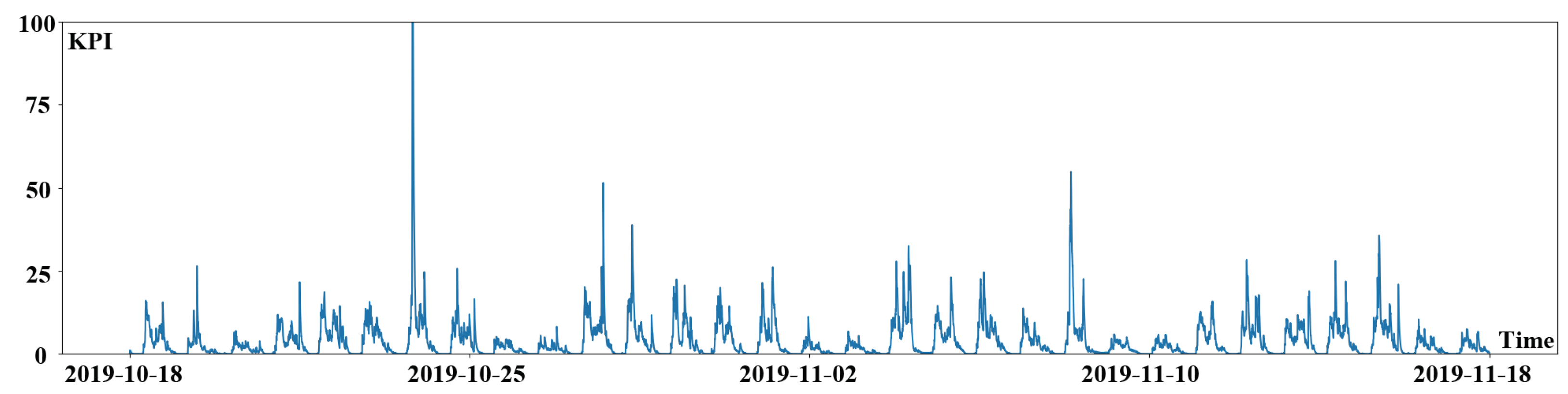
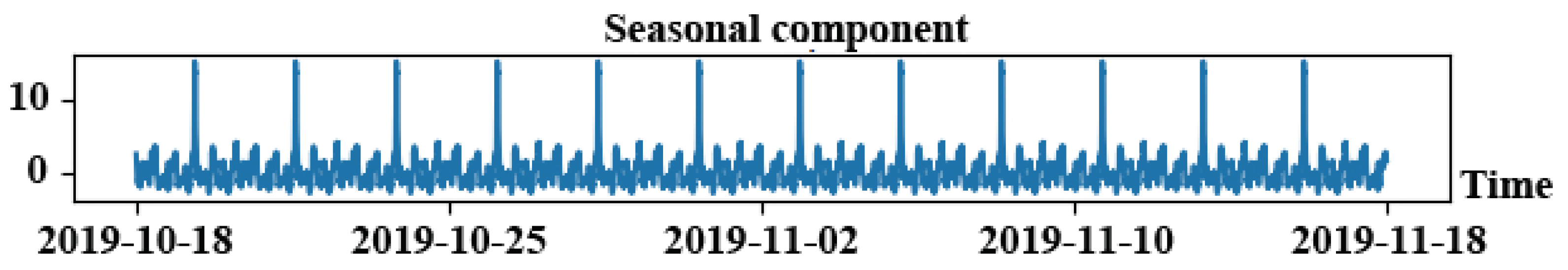
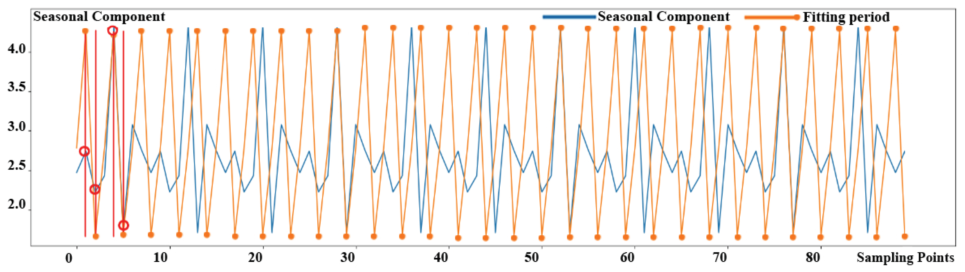
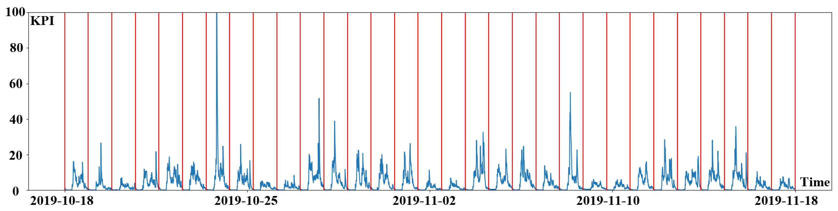
After determining the seasonal length, the original KPI time series data could be split into many sub-sequences. The segmented KPI sequence data is shown in Figure 5. KPI time series data is denoted by the blue line in the picture, whereas segmentation is represented by the red line. The following content is the procedure for clustering sub-sequences. To begin, calculate the distance between the KPI time series data sub-sequences by using a new lightweight distance measurement algorithm. Then cluster the sub-sequences by using DBSCAN clustering technique.

3.2.1. Lightweight Distance Measurement Algorithm

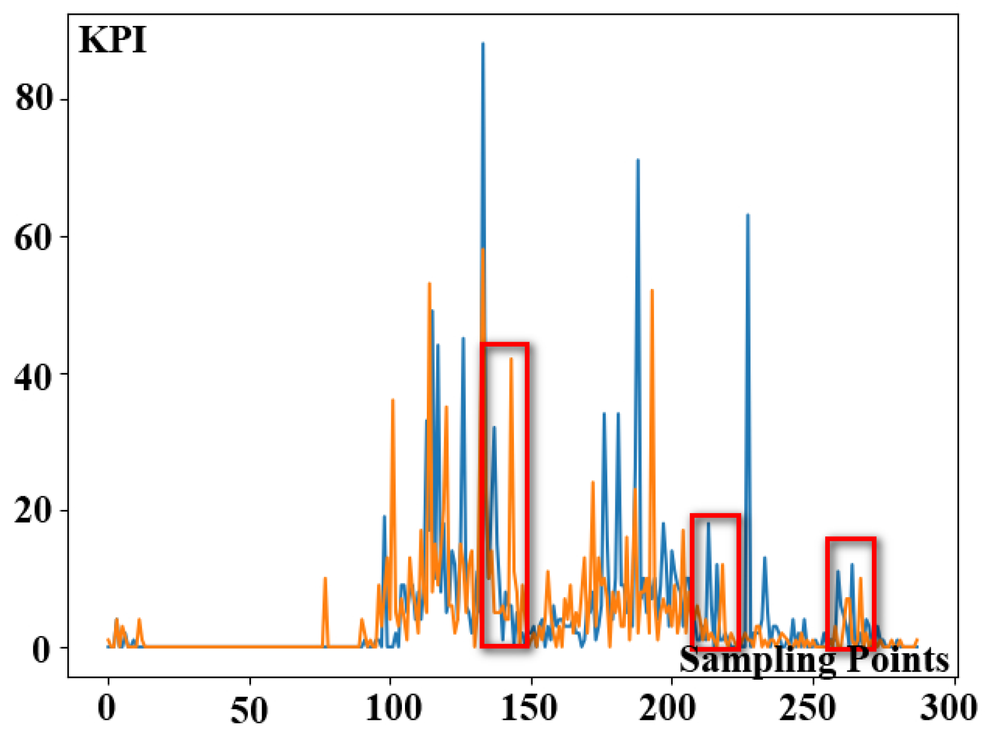
The choice of distance measurement algorithm has an important influence on the clustering algorithm [28]. In the previous literature, researchers have presented a variety of distance measurement algorithms, such as Move-Split-Merge [29], Spade [30], $L_p$ norm [31] and so on. Wang [32] evaluated nine distance measurement algorithms and corresponding derivative algorithms. Therefore, they discovered that Euclidean distance is more accurate than other distance measurement algorithms, and that DTW outperforms them. There is a significant variance in the direct use of Euclidean distance for distance measurement due to the offset of the KPI time series data. The offset phenomenon of KPI time series data is shown in Figure 6. In the picture, we use two color lines to represent two separated dates of KPI time series data. Furthermore, the peak values in the two pieces of KPI time series data shown in red rectangles are not perfectly aligned in time, indicating the offset phenomena of KPI time series data. DTW can handle the offset of KPI time series data, but the computation time will be very long because a large number of short sample intervals exist in intricate KPI time series data. Therefore, it is not appropriate to use the DTW algorithm directly under intricate KPI profiles.

To reduce time consumption of the clustering algorithm [33], we propose a lightweight distance measurement algorithm in ASAD to quantify the distance between KPI time series data sub-sequences. It can reduce the consuming time by extracting the primary information from a piece of KPI time series data and then utilizing the DTW method to estimate the distance. In short, there are three phases in this algorithm. Firstly, divide time series data into a set of data blocks. Secondly, modify each data block by using the discrete cosine transform, and the most important information is gathered in the upper left corner. Finally, extract the most significant data using a quantitative approach and matrix division. Following the above steps, we can extract the essential information and mask the offset of some KPI time series data to compress the sequence length.

The specific algorithm flow is as follows. At first, divide the data by one window size (n) for a given period of time series data. For example $n=8$, for the observed data of $Y=\{y_1,y_2,y_3,\cdots ,y_t\}$, divide Y into $8\times 8$ matrices. If the last matrix has less than $8\times 8$ elements, fill it with 0. After completing the previous step, the data in each window can form a matrix $M_i$, i = 1, 2, 3..., $\lceil \frac{len\left(Y\right)}{size}\rceil$, $M_i$ can be expressed as

$$M_i=\left[\begin{array}{cccc}{y}_{1+size\times (i-1)}& y_{2+size\times (i-1)}& \cdots & y_{8+size\times (i-1)}\\ y_{9+size\times (i-1)}& y_{10+size\times (i-1)}& \cdots & y_{16+size\times (i-1)}\\ ⋮& ⋮& \ddots & ⋮\\ y_{57+size\times (i-1)}& y_{58+size\times (i-1)}& \cdots & y_{64+size\times (i-1)}\end{array}\right]$$

(8)

Then, the discrete cosine transform is performed on the divided data block $M_i$.

$$D=UM{U}^T$$

(9)

where U is a discrete cosine variable matrix.

In our method, the discrete cosine variable matrix can be expressed as

$$U_{ij}=\left\{\begin{array}{c}\frac{1}{2^2\sqrt{2}},i=1\hfill \\ \frac{1}{2}cos[\frac{\pi }{16}(i-1)(2j-1)],i\ne 1\hfill \end{array}\right.$$

(10)

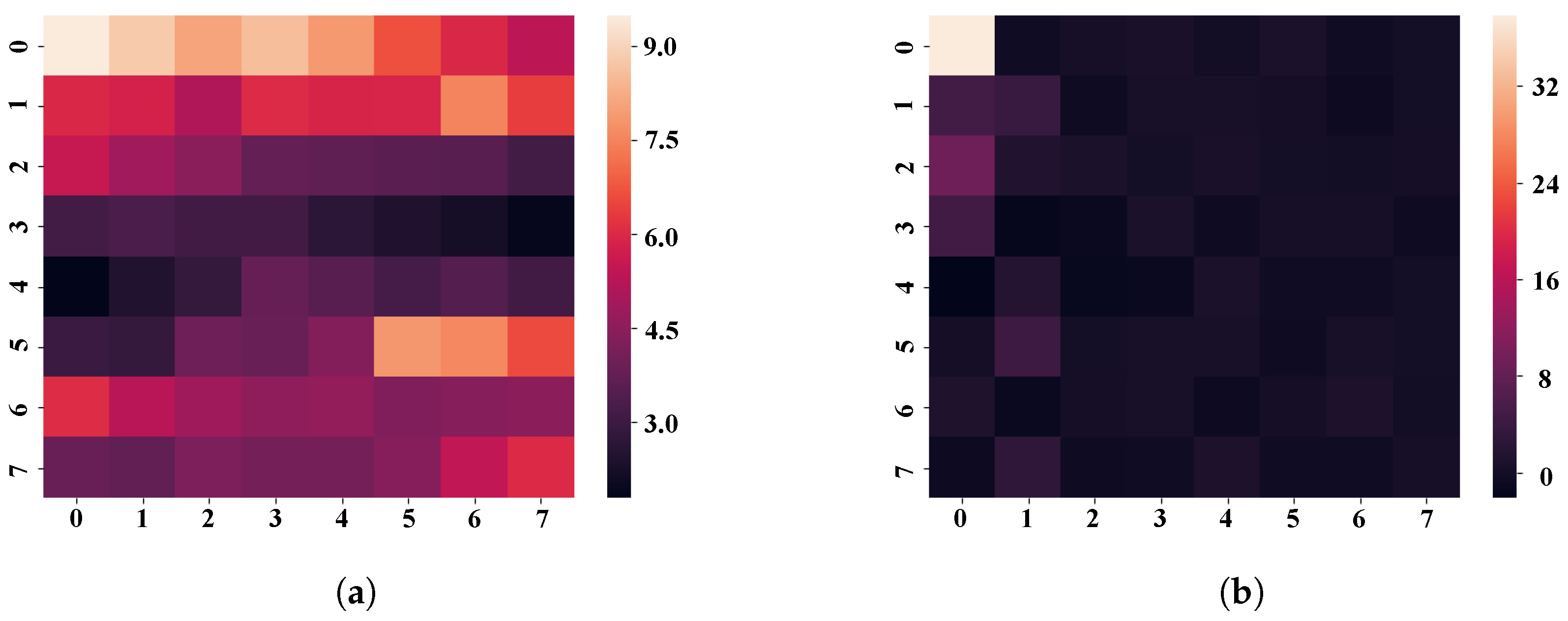
Taking one of the matrices as an example, the data aggregation effect of $M_i$ is shown in Figure 7. The color closest to white in the heat map represents a bigger absolute value of the data, whereas the color closest to black suggests a smaller absolute value of the data. The thermal data distribution of the original matrix is shown in Figure 7a. It can be seen that the original matrix’s data distribution is not concentrated, and the four corners of the matrix have more data. The thermal distribution of the data after the discrete cosine transform is shown in Figure 7b. Discrete cosine transform can express a finite time series sequence of KPI data in terms of a sum of cosine functions oscillating at different frequencies. The use of cosine rather than sine functions is critical for compression, since it turns out that fewer cosine functions are needed to approximate a typical signal, whereas for differential equations the cosines express a particular choice of boundary conditions. According to observations, the larger data in the updated matrix is predominantly dispersed in the upper left, while the absolute values of data scattered in other places are close to zero. As a result, the major data information in the matrix converges in the upper-left corner.

After the discrete cosine transform, quantify and divide the matrix, then determine the eigenvalues. The matrix D’s quantization matrx Q is as follows.

$$Q=round\left(\frac{D}{Z}\right)$$

(11)

where $round$ is rounding function and Z is the standard quantization matrix for discrete cosine transform [34].

For the matrix Q, it can be divided into four small matrices.

$$Q=\left[\begin{array}{cc}{q}_{11}& q_{12}\\ q_{21}& q_{22}\end{array}\right]$$

(12)

Because the matrix Q is generated by converging the principal information of the matrix D to the top-left corner, it can be seen that the matrix $q_{11}$ keeps the main data information and the matrix $q_{22}$ barely retains it in the figure. The highest values of the matrices $q_{12}$ and $q_{21}$ surpass the minimum value of the matrix $q_{11}$, indicating that the matrices $q_{12}$ and $q_{21}$ maintain the secondary information of the data. As a result, the matrix Q is represented as when the matrices $q_{12}$ and $q_{21}$ include the secondary information of the data.

$$Q\approx \left[\begin{array}{cc}{q}_{11}& q_{12}\\ q_{21}& 0\end{array}\right]$$

(13)

where we calculate the eigenvalues of the matrices $q_{11}$, $q_{12}$ and $q_{21}$, sort them in descending order to form an array as the principal information extracted from $M_i$.

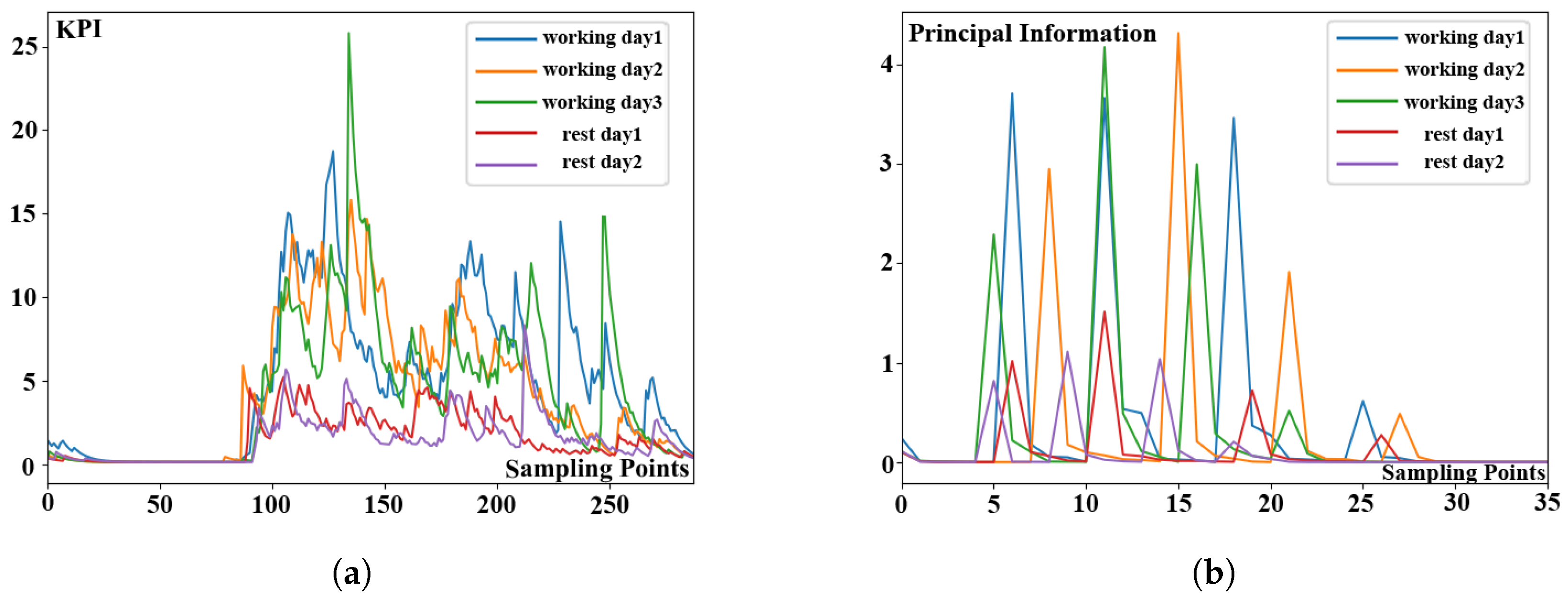
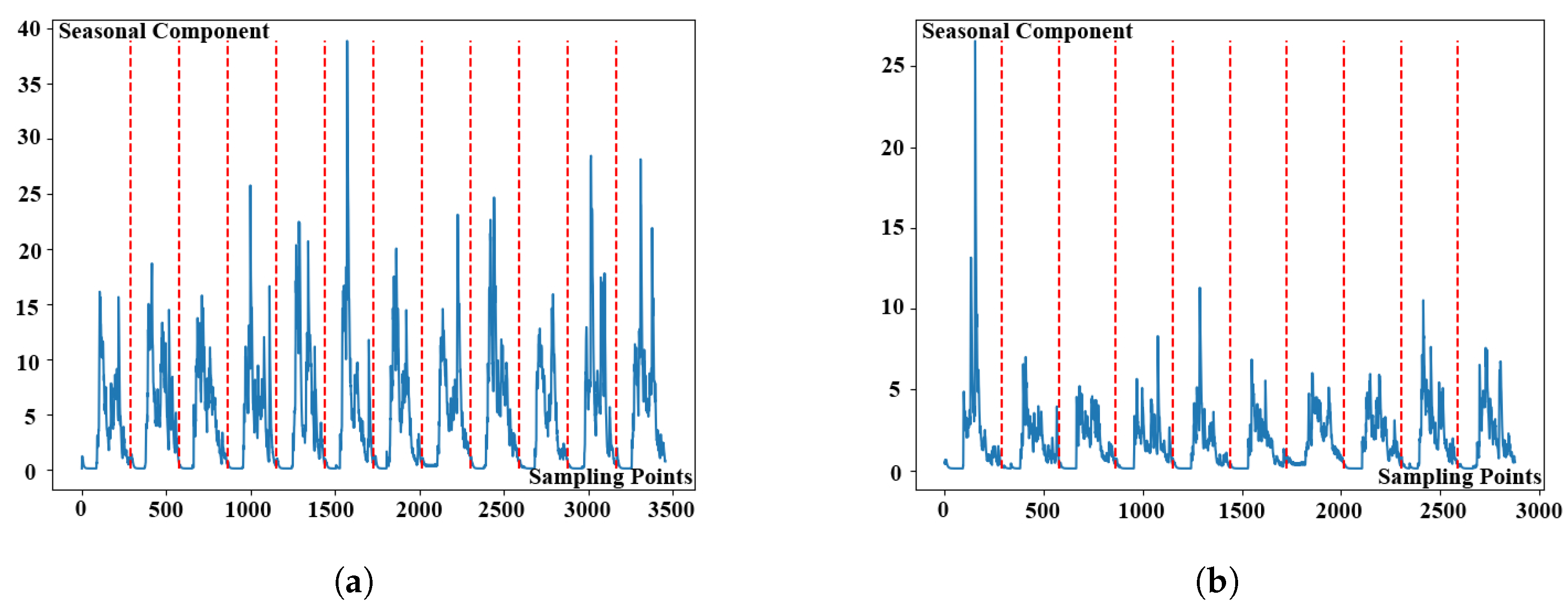
The comparison charts before and after extracting principal information of KPI time series data sub-sequences are shown in Figure 8. The KPI time series data sub-sequences segmented by day are shown in Figure 8a. The five different color sub-sequences in the figure represent different working days and rest days. Each of sub-sequences contains 288 observations. According to experimental results, KPI profiles of these three sub-sequences representing the working days are more similar. Similarly, the profiles of other two sub-sequences representing rest days are more similar. The KPI time series data sub-sequences after extracting the principal information are shown in Figure 8b. Five sub-sequences with various colors reflect distinct working days and rest days in the diagram. Each sub-sequence concludes 36 observations once the principal information has been extracted. Based on experimental observations, the analytical results are as follows. It can be seen that the data length of sub-sequences can be compressed by 87.5% without compromising profile similarity. Then, we use the classical DTW algorithm to calculate the distance between different sub-sequences because of the short length of extracted KPI time series data. As a result, we can say that our lightweight distance measurement algorithm is useful for reducing the clustering time consumption by extracting principal information from origin KPI time series data.

3.2.2. DBSCAN Clustering Algorithm

The second step in ASAD is an unsupervised learning technique to cluster the sub-sequences. When the samples are not labeled, it may divide the data into various clusters. The clustering process is based on calculating the distance between the data points. According to previous studies, there are two main clustering algorithms available for ASAD. K-means and DBSCAN are two of the most widely used clustering methods. The k-means algorithm is a traditional clustering algorithm that requires the number of groups to be specified. On the contrary, DBSCAN clustering algorithm does not need to determine the number of clustering centers. DBSCAN can cluster KPI time series data automatically based on the density of data points by setting the minimum number of clustering points and the clustering distance radius, rather than the number of clusters.

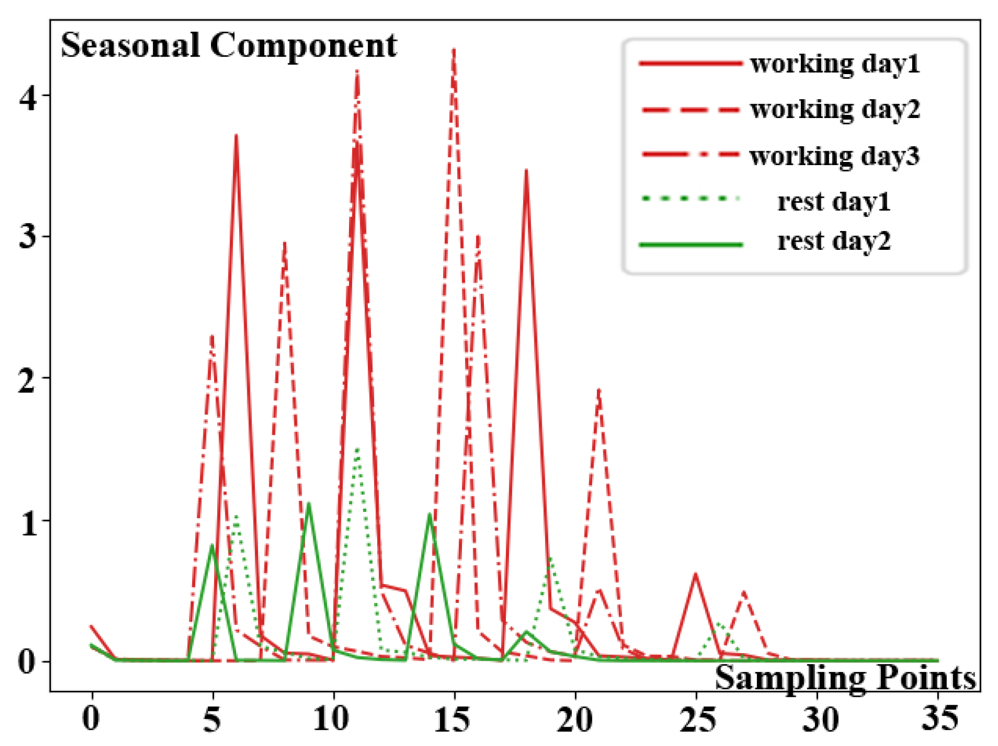
The result of DBSCAN clustering algorithm is shown in Figure 9. Five separate KPI time series data sub-sequences are shown in the figure by five different lines with varied patterns. Moreover, they are divided into two groups after being calculated using the DBSCAN clustering technique, which are denoted by red and green respectively. The working day mode is represented by the red KPI time series data sub-sequences, while the rest day mode is represented by the green KPI time series data sub-sequences. According to the experimental results, the similar KPI profiles among three sub-sequences in red belong to one category, while similar profiles between the two sub-sequences in green belong to another category. Meanwhile, it is worth noting that the clustering results corroborate the observations.

3.3. Calendar Based Correction Method

As shown in Figure 9, there are two categories of KPI time series data in those five KPI time series data sub-sequences, called working day mode and rest day mode. However, noise, abnormalities and other affecting factors may exist in the actual KPI time series data, leading to an inaccurate clustering result. So, we will put forward an improved method by integrating the calendar feature into ASAD, because KPI time series data is closely tied to time.

Firstly, we arrange the clustering results in row-first order according to the calendar as shown in

Table 3. Clustering results of KPI time series data sub-sequences.

Mon	Tue	Wed	Thu	Fri	Sat	Sun
				0	1	1
2	0	0	−1	0	1	1
−1	0	0	0	−1	1	1
−1	0	0	1	−1	1	1
0	0	2	0	−1	1	1

, where different numbers in the table indicate the category number corresponding to each KPI time-series data sub-sequences, and −1 indicates the noise category. Each cell in the table indicates the position of the KPI time series data sub-sequence in a week, and each row of the table represents a week. Specifically, calendar cell size is the same as seasonal length. Each column in the table reflects the same day of the week and has the same calendar property. Then, we follow these three steps to improve the clustering results. To begin, delete any data from the clustering result that is considered noise in

Table 4. Effective clustering results of KPI time series data sub-sequences.

Mon	Tue	Wed	Thu	Fri	Sat	Sun
				0	1	1
2	0	0	–	0	1	1
–	0	0	0	–	1	1
–	0	0	1	–	1	1
0	0	2	0	–	1	1

. The reason for this step is that the KPI time series data sub-sequences corresponding to these clustering findings may be anomalous, and statistical involvement will impair the clustering results’ correctness. Second, using the column as a unit, calculate the probability that each column belongs to a specific category as shown in

Table 5. Category probability statistics of KPI time series data sub-sequences.

	Mon	Tue	Wed	Thu	Fri	Sat	Sun
category 0	0.5	1	0.75	0.66	1	0	0
category 1	0	0	0	0.33	0	1	1
category 2	0.5	0	0.25	0	0	0	0

. Finally, determine the most likely categories of different calendar features based on the calendar characteristics. If many equally valid categories exist, the one with the most components is chosen. Hence, the final classifications only include category 0 and category 1 based on previous processes. To sum up, the KPI time series data sub-sequences from Monday to Friday are classified as category 0, whereas the KPI time series data sub-sequences on Saturday and Sunday are classified as category 1. In other words, category 0 is referred to as the working day mode, and category 1 is referred to as the rest day mode.

The KPI time series data sub-sequences of the same pattern are spliced in chronological order once the clustering results are corrected. The working day mode’s data and the rest day mode’s data spliced by the KPI time series data sub-sequences are shown in Figure 10a and Figure 10b, respectively. The spliced KPI time series data is shown by the blue line in the figure. Different KPI time series data sub-sequences are separated by the red line. According to observations, sub-sequences in each mode have a more consistent profile with other sub-sequences in the same mode, and the average value of working day mode is higher than the rest day mode’s.

4. Results

This subsection examines the performance of ASAD algorithm by designing the following evaluations. The experimental evaluation of the ASAD algorithm is mainly to verify its Seasonal Adaption, Time and Performance and F1-score. Seasonal Adaption consists of seasonal adaptive function and seasonal length evaluations. Time and Performance includes clustering time consumption and clustering accuracy of sub-sequences. F1-score is the overall performance indicator of our KPI anomaly detection algorithm ASAD.

4.1. Data Set Description

This work collects five KPI time series datasets from the private back-end system and Tencent cloud computing platform in order to validate the effect of the ASAD algorithm, and these data have been marked by engineers using the TRAINSET auxiliary tool. The time series data collected for KPIs includes indications such as system transactions, CPU utilization, IO, memory utilization and network traffic. A single indicator’s overall monitoring time ranges from 2 months to half a year, with a total time of more than 400 days.

Table 6. KPI indicator statistics of experimental dataset.

ID	Index Name	Sampling Interval (s)	Total Duration (Day)
A	Transactions per Second	300	180
B	CPU utilization	300	60
C	Number of full table scans Second	300	60
D	Memory utilization	300	60
E	Number of TCP connections	300	60

displays the KPI time series data gathered during this trial. The KPI in the table is highly relevant to the business and can indicate the system’s degree of irregularity. These KPI time series data are heavily influenced by user behavior and are roughly seasonal after manual assessment. In addition, the following statements are the features of these manually picked datasets. Dataset A has complicated categories, dataset B has evident seasonal features and less noise, dataset C has a lot of noise and is not obvious in seasons, dataset D has a seasonal length of more than 1 day and dataset E has a seasonal length of 1 day.

4.2. Seasonal Adaption Evaluation

First, we assess the ASAD algorithm’s seasonal adaptation function. With respect to seasonal adaptation functions, we compare the ASAD method to similar anomaly detection algorithms as shown in

Table 7. Seasonal adaptive function comparison.

	Argus	EGADS	Period	ASAD
Manually configure	✓	✓	✓	✓
Auto-configure			✓	✓
Seasonality adaptation				✓

. The seasonal length detection function of the KPI anomaly detection algorithm is gradually growing toward intelligence, from manual and automatic configuration of seasonal parameters to the process of self-adaptation. Both Argus and EGADS, according to tests, require human configuration of the seasonal length as a parameter in KPI anomaly detection and are unable to achieve seasonal adaptation. Period does not require the seasonal length parameter to be configured, but it is unable to adapt to the seasonal feature, because Period assumed that KPI time series data have a seasonal length of 1 day. As a result, only the ASAD algorithm has seasonal adaptive capability to detect anomalies under an intricate KPI profile.

Second, we evaluate the accuracy of the ASAD algorithm’s seasonal length detection. There are no other anomaly detection algorithms to compare, so we use auto-correlation as the comparison method. We divide the KPI time series data into multiple segments with a length of 1 week to half a month to test the performance.

Finally, we employ the ASAD method and auto-correction to determine the seasonal length of each test instance. According to

Table 8. Results of seasonal length evaluation.

	ASAD	Auto-Correction
Accuracy Rate	75%	43%
Error Rate	25%	57%

, ASAD algorithm has the 75% accuracy rate for detecting seasonal length. The auto-correction algorithm’s accuracy rate for detecting seasonal length is only 43%. The accuracy rate of the ASAD algorithm is higher than that of auto-correction, and the ASAD algorithm’s error rate is lower than that of auto-correction. To summarize, ASAD algorithm with a higher detection accuracy rate is better than auto-correction method for automatically detecting the seasonal length.

4.3. Time Overhead Evaluation

In this section, we firstly compare the time overhead of ASAD with Argus [3], EGADS [6] and Period [7]. Based on the single variable principle of the experiments, ASAD and Period both rely on EGADS as the anomaly detection model.

As shown in

Table 9. Time and performance comparison.

Algorithm	Average Time (s)
Argus	219
EGADS	51
Period	29
ASAD	39
Algorithm	Clustering Accuracy
Period	57%
ASAD	84%

, the overall KPI anomaly detection consuming time of ASAD, Period, EGADS and Argus is shown. It needs to be emphasized that time overhead is the average consuming time for detecting 1-month KPI time series data. According to the testing data, the anomaly detection consuming time of ASAD is 82% lower than Argus and 24% lower than EGADS, but it is a little higher than Period. We think this is due to the different clustering algorithms, so we do extra experiments to compare the clustering performance of sub-sequences. Moreover, in Table 9, it can be seen that the clustering accuracy of ASAD has reached 84%, while the clustering accuracy rate of Period is only 57%; that is to say, the clustering accuracy rate of ASAD is 27% higher than Period algorithm. This shows that the ASAD algorithm is more accurate for data clustering under intricate KPI profile.

According to the above experiments, we can see that time overhead of ASAD is the lowest of almost all algorithms. Although ASAD is a little slower than Period, it has a modest time overhead in return for more accurate sub-sequence clustering results. Furthermore, it also leads to the conclusion that the anomaly detection performance of our ASAD algorithm is better than Period algorithm in next section.

4.4. KPI Anomaly Detection Evaluation

In the application of KPI anomaly detection, fragmented alarms are more practical, so the statistics in this section take the form of fragmented alarms. The fragmented alarm processing process is as follows. The abnormality in the nearby and continuous time window is deemed a hit in the abnormal monitoring procedure if an anomaly is identified in the KPI time series data at a certain point. Specifically, the fragmented alarm is shown in Figure 11. The original KPI time series data is represented by the first row of data in the graphic, and each square represents one sampling point at a time. If a point is found to be abnormal, it is given a value of 1, otherwise it is given a value of 0. The anomaly score computed by the KPI anomaly detection algorithm is in the second row of data, and data in each square is the anomaly score at the corresponding time point. The discovered findings are indicated in the third row of data, and a point is considered abnormal if the abnormal score exceeds a particular threshold. The experimental statistical results are in the fourth line of data, which are fine-tuned by fragmented alarm [13]. The adjusted statistical result are Recall = 50%, Precision = 50% and F1-Score = 0.5.

This section analyzes the effects of ASAD, Period, EGADS and Argus for KPI anomaly detection in order to assess the overall effect of KPI anomaly detection. We also utilize F1-Score as a comparative metric because it can synthetically reflect algorithm quality. Each dataset is separated into numerous samples of 1 month in length for the experiment. Argus, EGADS, Period and ASAD are four algorithms that are evaluated on several samples of diverse datasets. The recall rate, accuracy and F1-scores of each algorithm on various datasets are shown in Figure 12. According to the analysis on most datasets, the F1-score of the ASAD method is higher than the other three algorithms. Only on dataset E is the ASAD algorithm’s F1-score slightly lower than Period’s F1-score.

4.5. Experimental Analysis

Primarily, the ASAD algorithm can achieve seasonal adaptation. However, Argus and EGADS require human setting of the seasonal length, and Period can only generate one seasonal length for all current data. Simultaneously, ASAD’s seasonal length computation accuracy might reach 75%, which is better than the auto-correction technique.

Furthermore, the ASAD algorithm performs well with respect to both time consumption and sub-sequence clustering accuracy. Despite the fact that the ASAD algorithm consumes somewhat more time than the Period algorithm, its clustering accuracy rate is significantly higher.

Finally, because the Period and ASAD outperform the Argus and EGADS in terms of recall, accuracy, and F-score on each KPI, the comparison and analysis of the Period and the ASAD are the focus of attention in terms of dataset features. In Figure 12, it can be seen that ASAD outperforms Period in 80% of KPI datasets.

5. Conclusions

In this work, we present ASAD, a seasonal adaptive KPI anomaly detection algorithm. To begin, ASAD used a scaling Auto-Period algorithm to create a set of seasonal sub-sequences. Meanwhile, sub-sequence clustering is optimized using eBeats clustering algorithm and calendar-based correction method. Then, using the above clustering results, train several offline anomaly detection models. Finally, choose an appropriate offline model to detect KPI anomaly for online data based on the derived seasonal information. Experiments demonstrate that ASAD can achieve seasonal adaptation effect and enhance overall KPI anomaly detection performance under intricate KPI profiles.

However, KPI time series data could contain multiple seasonal lengths and one abnormality does not necessarily indicate that the overall system is abnormal. Therefore, we are dedicated to study multiple seasonal lengths detection and correlation among many KPI anomalies. Future work would further improve KPI anomaly detection accuracy.

References

1. He, S.; Li, Z.; Wang, J.; Xiong, N.N. Intelligent Detection for Key Performance Indicators in Industrial-Based Cyber-Physical Systems. IEEE Trans. Ind. Inform. 2021, 17, 5799–5809. [Google Scholar] [CrossRef]
2. Wu, D.; Zhou, D.; Chen, M.; Zhu, J.; Yan, F.; Zheng, S.; Guo, E. Output-Relevant Common Trend Analysis for KPI-Related Nonstationary Process Monitoring With Applications to Thermal Power Plants. IEEE Trans. Ind. Inform. 2021, 17, 6664–6675. [Google Scholar] [CrossRef]
3. He, Y.; Flavel, A.; Ge, Z.; Gerber, A.; Massey, D.; Papadopoulos, C.; Shah, H.; Yates, J. Argus: End-to-end service anomaly detection and localization from an isp’s point of view. In Proceedings of the 2012 Proceedings IEEE INFOCOM, Orlando, FL, USA, 25–30 March 2012; pp. 2756–2760. [Google Scholar]
4. Chen, Y.; Mahajan, R.; Sridharan, B.; Zhang, Z.L. A provider-side view of web search response time. ACM Sigcomm Comput. Commun. Rev. 2013, 43, 243–254. [Google Scholar] [CrossRef]
5. Liu, D.; Zhao, Y.; Xu, H.; Sun, Y.; Pei, D.; Luo, J.; Jing, X.; Feng, M. Opprentice: Towards practical and automatic anomaly detection through machine learning. In Proceedings of the 2015 Internet Measurement Conference, Tokyo, Japan, 28–30 October 2015; pp. 211–224. [Google Scholar]
6. Laptev, N.; Amizadeh, S.; Flint, I. Generic and scalable framework for automated time-series anomaly detection. In Proceedings of the 21th ACM SIGKDD International Conference on Knowledge Discovery and Data Mining, Sydney, Australia, 10–13 August 2015; pp. 1939–1947. [Google Scholar]
7. Zhao, N.; Zhu, J.; Wang, Y.; Ma, M.; Zhang, W.; Liu, D.; Zhang, M.; Pei, D. Automatic and Generic Periodicity Adaptation for KPI Anomaly Detection. IEEE Trans. Netw. Serv. Manag. 2019, 16, 1170–1183. [Google Scholar] [CrossRef]
8. Chen, W.; Xu, H.; Li, Z.; Pei, D.; Chen, J.; Qiao, H.; Feng, Y.; Wang, Z. Unsupervised anomaly detection for intricate kpis via adversarial training of vae. In Proceedings of the IEEE INFOCOM 2019-IEEE Conference on Computer Communications, Paris, France, 29 April–2 May 2019; pp. 1891–1899. [Google Scholar]
9. Ch, V.; Banerjee, A.; Kumar, V. Anomaly detection: A survey. ACM Comput. Surv. (CSUR) 2009, 41, 15. [Google Scholar]
10. Hyndman, R.J.; Athanasopoulos, G. Forecasting: Principles and Practice; OTexts: Melbourne, Australia, 2018. [Google Scholar]
11. Wang, Y.; Wang, Z.; Xie, Z.; Zhao, N.; Pei, D. Practical and White-Box Anomaly Detection through Unsupervised and Active Learning. In Proceedings of the 29th International Conference on Computer Communications and Networks (ICCCN), Honolulu, HI, USA, 3–6 August 2020. [Google Scholar]
12. Yaacob, A.H.; Tan, I.K.T.; Chien, S.F.; Tan, H.K. Arima based network anomaly detection. In Proceedings of the 2010 Second International Conference on Communication Software and Networks, Singapore, 26–28 February 2010; pp. 205–209. [Google Scholar]
13. Fang, Z.; Cheng, Q.; Mou, L.; Qin, H.; Zhou, H.; Cao, J. Abnormal electricity consumption detection based on ensemble learning. In Proceedings of the 2019 9th International Conference on Information Science and Technology (ICIST), Hulunbuir, China, 2–5 August 2019; pp. 175–182. [Google Scholar]
14. Himeur, Y.; Alsalemi, A.; Bensaali, F.; Amira, A. A novel approach for detecting anomalous energy consumption based on micro-moments and deep neural networks. Cogn. Comput. 2020, 12, 1381–1401. [Google Scholar] [CrossRef]
15. Himeur, Y.; Elsalemi, A.; Bensaali, F.; Amira, A. Detection of appliance-level abnormal energy consumption in buildings using autoencoders and micro-moments. In Proceedings of the Fifth International Conference on Big Data and Internet of Things (BDIoT), Rabat, Morocco, 17–18 March 2021; pp. 1–13. [Google Scholar]
16. Deng, A.; Hooi, B. Graph neural network-based anomaly detection in multivariate time series. Proc. Aaai Conf. Artif. Intell. 2021, 35, 5. [Google Scholar]
17. Chen, Z.; Chen, D.; Zhang, X.; Yuan, Z.; Cheng, X. Learning graph structures with transformer for multivariate time series anomaly detection in iot. IEEE Internet Things J. 2022, 12, 9179–9189. [Google Scholar] [CrossRef]
18. Zhou, Y.; Ren, H.; Li, Z.; Pedrycz, W. An anomaly detection framework for time series data: An interval-based approach. Knowl.-Based Syst. 2021, 228, 107153. [Google Scholar] [CrossRef]
19. Xu, H.; Chen, W.; Zhao, N.; Li, Z.; Bu, J.; Li, Z.; Liu, Y.; Zhao, Y.; Pei, D.; Feng, Y.; et al. Unsupervised anomaly detection via variational auto-encoder for seasonal kpis in web applications. In Proceedings of the 2018 World Wide Web Conference, Lyon, France, 23–27 April 2018; pp. 187–196. [Google Scholar]
20. Himeur, Y.; Alsalemi, A.; Bensaali, F.; Amira, A. Smart power consumption abnormality detection in buildings using micromoments and improved K-nearest neighbors. Int. J. Intell. Syst. 2021, 36, 2865–2894. [Google Scholar] [CrossRef]
21. Li, J.; Izakian, H.; Pedrycz, W.; Jamal, I. Clustering-based anomaly detection in multivariate time series data. Appl. Soft Comput. 2021, 100, 106919. [Google Scholar] [CrossRef]
22. Li, J.; Di, S.; Shen, Y.; Chen, L. FluxEV: A fast and effective unsupervised framework for time-series anomaly detection. In Proceedings of the 14th ACM International Conference on Web Search and Data Mining, Virtual, 8–12 March 2021; pp. 824–832. [Google Scholar]
23. Carmona, C.U.; Aubet, F.X.; Flunkert, V.; Gasthaus, J. Neural contextual anomaly detection for time series. arXiv 2021, arXiv:2107.07702. [Google Scholar]
24. Himeur, Y.; Ghanem, K.; Alsalemi, A.; Bensaali, F.; Amira, A. Anomaly detection of energy consumption in buildings: A review, current trends and new perspectives. Appl. Energy 2020, 289, 116601. [Google Scholar]
25. Thill, M.; Konen, W.; Wang, H.; Bäck, T. Temporal convolutional autoencoder for unsupervised anomaly detection in time series. Appl. Soft Comput. 2021, 112, 107751. [Google Scholar] [CrossRef]
26. Clevel, R.B.; Clevel, W.S.; McRae, J.E.; Terpenning, I. STL: A Seasonal-Trend Decomposition Procedure Based on Loess. J. Off. Stat. 1990, 6, 3–73. [Google Scholar]
27. Vlachos, M.; Yu, P.; Castelli, V. On periodicity detection and structural periodic similarity. In Proceedings of the 2005 SIAM International Conference on Data Mining, Newport Beach, CA, USA, 21–23 April 2005; Society for Industrial and Applied Mathematics: Philadelphia, PA, USA, 2005. [Google Scholar]
28. Paparrizos, J.; Gravano, L. k-shape: Efficient and accurate clustering of time series. In Proceedings of the 2015 ACM SIGMOD International Conference on Management of Data, Melbourne, VIC, Australia, 31 May–4 June 2015. [Google Scholar]
29. Stefan, A.; Athitsos, V.; Das, G. The move-split-merge metric for time series. IEEE Trans. Knowl. Data Eng. 2012, 25, 1425–1438. [Google Scholar] [CrossRef] [Green Version]
30. Chen, Y.; Nascimento, M.A.; Ooi, B.C.; Tung, A.K.H. Spade: On shape-based pattern detection in streaming time series. In Proceedings of the 2007 IEEE 23rd International Conference on Data Engineering, Istanbul, Turkey, 15–20 April 2007; pp. 786–795. [Google Scholar]
31. Chen, L.; Ng, R. On the marriage of lp-norms and edit distance. In Proceedings of the Thirtieth International Conference on Very Large Data Bases, Toronto, ON, Canada, 31 August–3 September 2004; Volume 30, pp. 792–803. [Google Scholar]
32. Wang, X.; Mueen, A.; Ding, H.; Trajcevski, G.; Scheuermann, P.I.; Keogh, E. Experimental comparison of representation methods and distance measures for time series data. Data Min. Knowl. Discov. 2013, 26, 275–309. [Google Scholar] [CrossRef] [Green Version]
33. Gonzalez-Vidal, A.; Barnaghi, P.; Skarmeta, A.F. BEATS: Blocks of Eigenvalues Algorithm for Time Series Segmentation. IEEE Trans. Knowl. Data Eng. 2018, 30, 2051–2064. [Google Scholar] [CrossRef] [Green Version]
34. Bovik, A.C. (Ed.) The Essential Guide to Image Processing; Academic Press: Cambridge, MA, USA, 2009. [Google Scholar]
Figure 1. The sample KPI time series data after data pre-processing.
Applsci 12 05855 g001
Figure 2. Seasonal components of KPI time series data.
Applsci 12 05855 g002
Figure 3. Seasonal components scaling.
Applsci 12 05855 g003
Figure 4. Period fitting of seasonal component data.
Applsci 12 05855 g004
Figure 5. Sub-sequences segmentation of KPI time series data.
Applsci 12 05855 g005
Figure 6. Cycle offset diagram of KPI time series data.
Applsci 12 05855 g006
Figure 7. Data aggregation comparison chart. (a) Data thermal distribution of the original matrix. (b) Data heat distribution of the aggregation matrix.
Applsci 12 05855 g007
Figure 8. The comparison before and after information extraction. (a) Sub-sequences before extracting the principal information. (b) Sub-sequences after extracting the principal information.
Applsci 12 05855 g008
Figure 9. Clustering result of KPI time series data sub-sequences.
Applsci 12 05855 g009
Figure 10. Mosaic of KPI time series data in different modes. (a) KPI time series data in working day mode. (b) KPI time series data in rest day mode.
Applsci 12 05855 g010
Figure 11. Fragment alarm for anomaly detection.
Applsci 12 05855 g011
Figure 12. Experimental comparison to other algorithms.
Applsci 12 05855 g012