Nonsynchronous Rotor Blade Vibrations in Last Stage of 380 MW LP Steam Turbine at Various Condenser Pressures

Abstract

This paper presents an analysis of nonsynchronous rotor blade vibrations in the last stage of an LP steam turbine at various condenser pressures. The nonlinear least squares Levenberg–Marquardt method is used in a tip-timing analysis to determine nonsynchronous multimode rotor blade vibrations, which is a novelty. This is done with two sensors in the casing and a once-per-revolution sensor. The accuracy of the nonlinear least squares Levenberg–Marquardt multimode method is compared with the one-mode linear method. The algorithm is verified by comparing it with one-mode tip-timing methods for synchronous and nonsynchronous vibrations. The analysis shows that the rotor blades vibrate simultaneously with two modes in non-nominal conditions, which is also a novelty. The rotor frequencies are unchanged, although the blade vibration amplitudes vary, depending on the pressure in the condenser. Flutter does not appear in the last stage for the various condenser pressures and powers that were tested.

1. Introduction

In the last stage of the LP steam turbine, rotor blades can vibrate with higher amplitudes as a result of flutter or changes in condenser pressure [1]. This paper considers rotor blade amplitudes and frequencies using the tip-timing method.

Measurements of steam turbine last stage LP rotor blade vibrations were presented by Rao and Dutta [2], using a noise sensor mounted in the casing to find the excessive blade vibration caused by flutter in high condenser pressure.

Donato et al. [3] used the tip-timing method with an optical sensor mounted in the casing to find blade vibration in an LP last stage.

The experimental and numerical results of the last-stage low-pressure rotor blade flutter were presented by Sanvito et al. [4]. The dynamic behavior of blades was numerically investigated, and the grouping of blades in packs was optimized to avoid resonances. This led to the design of new blades, which were mounted in the turbine, and the measured results showed an improvement in the turbine’s dynamic behavior.

Prochazka and Vanek [5] used tip-timing to show an increase in the vibration amplitude of a cracked blade in a 1000 MW turbine LP last stage.

Przysowa [6] used tip timing to analyze synchronous and nonsynchronous vibrations of a steam turbine LP last stage rotor blade. This showed how the pressure in the condenser influences rotor blade vibration in a nominal state.

This paper analyzes blade amplitudes and frequencies by varying the condenser pressure and power to non-nominal conditions in the steam turbine LP last stage, which is a new approach. The condenser pressure is regulated by a valve breaking the vacuum in the exhaust hood. The nonlinear least-squares Levenberg–Marquardt tip-timing method is used to identify multimode blade vibrations.

A literature review of tip-timing methods was presented at ASME Turbo-Expo 2012, Copenhagen [7,8,9,10,11,12], and by Rzadkowski et al. [13].

Several processing techniques have been proposed for the blade tip-timing method, using various numbers of probes and probe configurations.

Some tip-timing studies have assumed that each blade vibrates with a single frequency mode [14,15,16].

An auto-based blade tip-timing (BTT) analysis method for blades vibrating with two simultaneous resonances was used by Gallego-Garrido et al. [17].

A method of analyzing multimode blade vibration signals involving groups of regularly spaced optical sensors was used by Beauseroy and Langelle [18]. Blade multi modes in a rotating stall were identified using the non-uniform Fourier transform by Kharyton and Bladh [19]. Most of the eigenmodes in the rotating stall were excited as the result of repeated, strong impacts on the blade. Eight optical probes were used. Kharyton et al. [20] used the non-uniform Fourier transform (NUDFT), the minimum variance spectrum estimator approach, a multichannel technique with in-between samples interpolation, the Lomb–Scargle periodogram and an iterative variable threshold procedure to analyze synchronous engine order resonance, rotating stall and limit-cycle oscillations. The synchronous analysis required a higher number of sensors. NUDFT methods estimated the first three nonsynchronous blade modes of a steam turbine for vibration. Sparse reconstruction of the blade tip-timing signal for multimode blade vibrations was proposed by Lin et al. [21]. Four sensors were sufficient to reconstruct the vibration signal for a numerical simulation of rotor blade vibration with three modes. In the experimental set-up, three optical sensors were mounted in the casing, and an additional optical fiber once-per-revolution sensor was also used. One-frequency blade vibrations were detected. The number of sensors depended on the sparseness of the blade vibration signal. In the worst case, the number of sensors was twice the number of dominant vibration frequencies. The influence of measurement uncertainties was not considered.

A novel approach based on the sparse representation theorem for the detection of multimode blade vibration frequencies with uncertainty reduction was presented by Pan et al. [22]. There, four sensors in the casing were used in experiments to recover the blade vibration spectra with acceptable accuracy.

Guo et al. [23] used the Levenberg–Marquardt (LM) theory to investigate synchronous blade vibrations using three sensors in the casing, but without a once-per-revolution sensor. If the EO was known, only two sensors were used. The blades were modelled to vibrate with a single-mode.

Wang et al. [24] proposed a coupled vibration analysis (CVA) where the least-squares Levenberg–Marquardt tip-timing method was used to identify mistuned blade synchronous vibration parameters. Although a CVA can be applied without a once-per-revolution sensor, at least four sensors are required. A single frequency blade vibration response was assumed. This method required the mistuned bladed disc where the blades are not identical as the result of manufacturing tolerances. When all the blades were identical (tuned), the results proved to be unreliable.

A two-sensor method of synchronous blade vibration analysis was presented by Fan et. al. [25], where two optical fiber probes were used without a once-per-revolution sensor. The nonlinear least-squares method was used to fit the curves of one-mode synchronous blade vibrations.

To identify synchronous blade vibrations, the least-squares Levenberg–Marquardt tip-timing method used in [24] and the nonlinear methods in [25] assumed a single frequency blade vibration response.

The nonlinear least-squares Levenberg–Marquardt method used in this paper determines asynchronous multimode blade vibration components, where the blade can vibrate simultaneously with several modes and frequencies—see Equation (4), which is a novelty. This algorithm was verified in comparison with other tip-timing methods [26,27,28] for synchronous and nonsynchronous blade vibrations. In the tip-timing analysis presented here, two sensors in the casing and a once-per-revolution sensor (Figure 1) were used. This also demonstrated the higher accuracy of the nonlinear least-squares Levenberg–Marquardt multimode method in comparison to the one-mode linear method.

2. Methodology

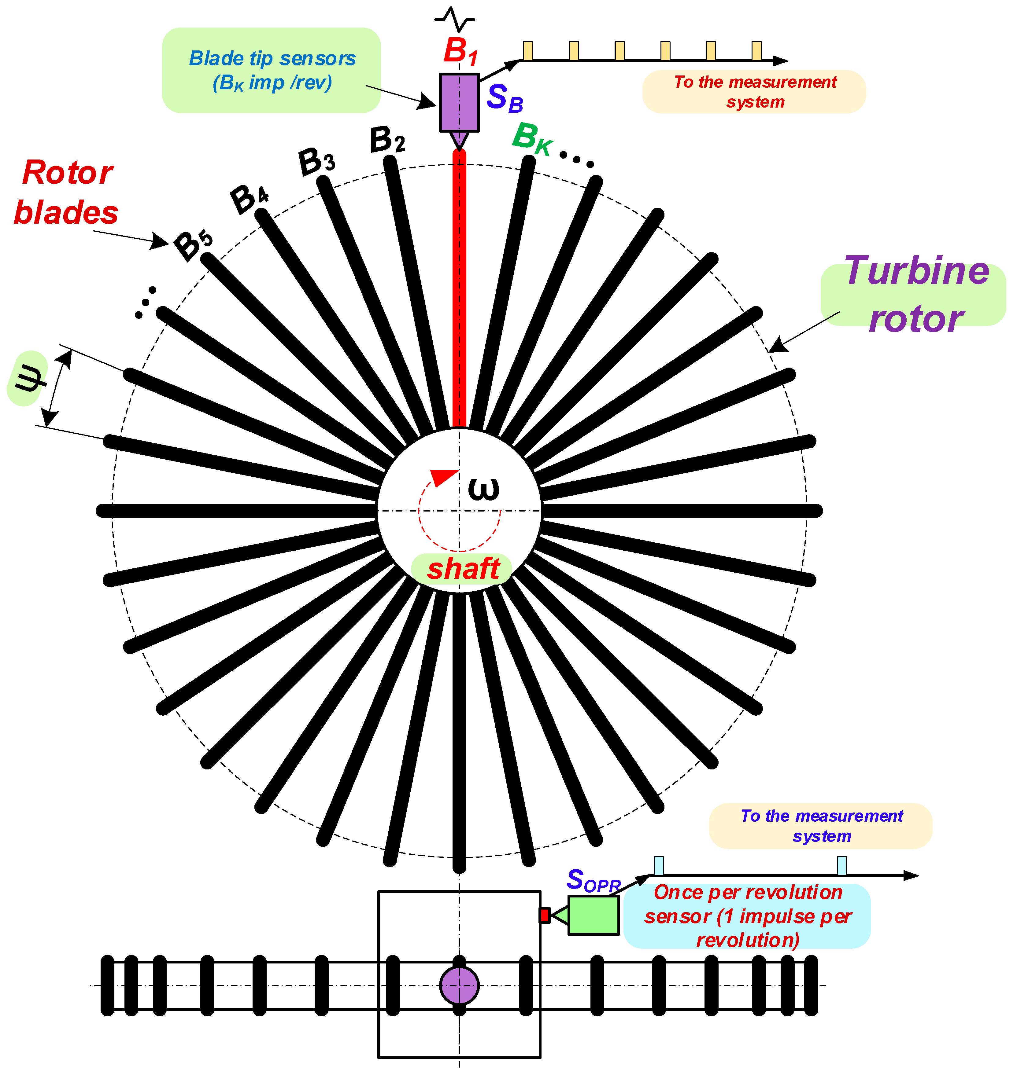
Blade displacements are calculated based on the times of blade arrival (Figure 1) measured using blade tip sensors (S_B) and a once-per-revolution sensor (S_OPR). These displacements are then used to calculate the harmonics of multimode rotor blade vibrations (A(t) in Equations (1)–(4))

To find the harmonics of multimode rotor blade vibrations using the tip-timing method, their amplitudes may be assumed as follows:

$$A\left(t\right)=A_0\sin \left(2\pi f_{o}t+\phi \right)+\tilde{0}\mathrm{one}\mathrm{harmonic}$$

(1)

$$A\left(t\right)=A_1\sin \left(2\pi f_{1}t+{\phi }_1\right)+A_2\sin \left(2\pi f_{2}t+{\phi }_2\right)+\tilde{0}\mathrm{two}\mathrm{harmonics}$$

(2)

$$\begin{array}{c}A\left(t\right)=A_1\sin \left(2\pi f_{1}t+{\phi }_1\right)+A_2\sin \left(2\pi f_{2}t+{\phi }_2\right)+A_3\sin \left(2\pi f_{3}t+{\phi }_3\right)+\tilde{0}\mathrm{three}\mathrm{harmonics}\end{array}$$

(3)

where: A(t) refers to the known values of blade displacements in time, A_i is the amplitude for i-th harmonic, f_i is the frequency of the blade vibrations for i-th harmonics, and t is the known time for which the displacement A(t) was calculated, φ_i is the phase shift for i-th harmonic, $\tilde{0}$ is the “0”- noise level of the blade vibrations. In the case of more harmonics:

$$A\left(t\right)={\displaystyle \sum }_i{A}_i\sin \left(2\pi f_{i}t+{\phi }_i\right)+\tilde{0},i=1,2,\dots$$

(4)

where: i is the number of harmonics.

Equations (1)–(4) adequately fit the measured data in the nonlinear least-squares method to obtain the amplitudes A_i, frequencies f_i and phases φ_i of i-th blade mode vibrations. The accuracy of each fitting can be calculated on the basis of the following average fitting error:

$$\epsilon =\frac{{{\displaystyle \sum }}_{i=0}^n\frac{|A_{im}-A\left(t_i\right)|}{\left|A_{im}\right|}}{n}$$

(5)

where: n is the number of points in the fitting sample, A_im is the i-th measured blade displacement in a sample, A(t_i) is the amplitude for the fitting function in i-th time from a sample and $\epsilon$ varies from 5 to 15%.

In the fitting for each blade, the smallest ε was chosen.

In the algorithm, the initial values have to be assumed. Some problems of ill-conditioning and divergence can be corrected by estimating initial parameters. This can be done for amplitude in sinusoidal motion Equation (1) by using [29]:

$$A_{0start}=\sqrt{2}{A}_{RMS}$$

(6)

where: A_RMS is the root mean square amplitude.

The noise level does not have to be a fitting parameter and can be calculated beforehand:

$$\tilde{0}=\frac{{{\displaystyle \sum }}_{i=0}^n{A}_{im}}{n}$$

(7)

where: A_im is the i-th measured blade displacement in a sample.

The noise level is a sum of all measured displacements for a blade in a fitting sample, divided by the number of points in the fitting sample.

It is impossible to estimate amplitudes in Equations (2)–(4), thus for each fitting attempt, an initial min-max value is randomly chosen:

$$\begin{gathered} A_{1start}=random\left(A_{1min},A_{1max}\right) \\ \begin{array}{c}{A}_{2start}=random\left(A_{2min},A_{2max}\right)\end{array} \\ {A}_{3start}=random\left(A_{3min},A_{3max}\right) \end{gathered}$$

(8)

The starting value frequencies are:

$$\begin{gathered} f_{start}=random\left(f_{min},f_{max}\right) \\ {f}_{1start}=random\left(f_{1min},f_{1max}\right) \\ {f}_{2start}=random\left(f_{2min},f_{2max}\right) \\ {f}_{3start}=random\left(f_{3min},f_{3max}\right) \end{gathered}$$

(9)

Finally, the phase may be assumed as:

$$\begin{gathered} {\phi }_{start}=random\left(0,\pi \right) \\ {\phi }_{1start}=random\left(0,\pi \right) \\ {\phi }_{2start}=random\left(0,\pi \right) \end{gathered}$$

(10)

3. Levenberg–Marquardt Algorithm

In fitting, the nonlinear least-squares Levenberg–Marquardt algorithm (L–M) is used [30].

This iterative algorithm is based on successive approximation of analyzed parameters (i.e., frequency, amplitude and phase):

$${\beta }_j^{k+1}={\beta }_j^k+\Delta {\beta }_j$$

(11)

where: ${\beta }_j^k$ is a parameter value of the blade mode (frequencies (j = 1) or amplitudes (j = 2) or phases (j = 3)), the superscript k is the iteration step, and the difference Δβ_j is called the shift value. At each iteration, the model is linearized using the Taylor series:

$$F\left(x_i,\mathbf{\beta }\right)=F^k\left(x_i,\mathbf{\beta }\right)+{\displaystyle \sum }_j\frac{\partial F\left(x_i,\mathbf{\beta }\right)}{\partial {\beta }_j}\left({\beta }_j-{\beta }_j^k\right)=F^k\left(x_i,\mathbf{\beta }\right)+{\displaystyle \sum }_j{J}_{ij}\Delta {\beta }_j$$

(12)

where: $\mathbf{\beta }$ is a vector of the parameters (frequency, amplitude and phase).

Jacobian J is a function of the constant (in this case, it is $\tilde{0}$ from Equations (1)–(4)), the independent variable (time) (x_i), and the parameters, and therefore changes from iteration to iteration.

The fitting error for each measurement is:

$$r_i=y_i-F^j\left(x_i,\mathbf{\beta }\right)-{\displaystyle \sum }_{j=1}^m{J}_{ij}\Delta {\beta }_j=\Delta y_i-{\displaystyle \sum }_{j=1}^m{J}_{ij}\Delta {\beta }_j$$

(13)

where: y_i is the measured value (blade displacement), i = 1, …, n, n is the number of measurement points, F is a function of the model (in this case, right side of Equation (1) or (2) or (3) or (4)), m is connected with the number of blade mode components m = 3 for one harmonic, 6 for two harmonics, etc., $\mathbf{\beta }$ is a vector of the parameters (frequency, amplitude and phase).

The sum of squared fitting errors is minimized

$$S={\displaystyle \sum }_i^n{r}_i^2$$

(14)

The minimum value of S occurs when the gradient is zero.

$$\frac{\partial S}{\partial {\beta }_j}=2{\displaystyle \sum }_i^n{r}_i\frac{\partial r_i}{\partial {\beta }_j}=0\left(j=1,\dots ,m\right)$$

(15)

Number of parameters m, means that there are m gradient equations,

${\beta }_j$ is approximated in each step using (11).

Next, Jacobian J is linearized:

$$J_{ij}=-\frac{\partial r_i}{\partial {\beta }_j}$$

(16)

Substituting (13) and (16) into (15):

$$-2{\displaystyle \sum }_{i=1}^n{J}_{ij}\left(\Delta y_i-{\displaystyle \sum }_{k=1}^m{J}_{ik}\Delta {\beta }_k\right)=0$$

(17)

where: n is the number of measurement points.

Equation (17) can be written as the m of linear equations:

$${\displaystyle \sum }_{i=1}^n{\displaystyle \sum }_{k=1}^m{J}_{ij}{J}_{ik}\Delta {\beta }_k={\displaystyle \sum }_{i=1}^n{J}_{ij}\Delta y_i\left(j=1,\dots ,m\right)$$

(18)

Equation (18) is analogous to the linear least squares fitting algorithm and can be easily solved.

The nonlinear least-squares Levenberg–Marquardt algorithm requires a gradient of Equation (1) or (2) or (3) or (4) (Jacobian J in the linearized model). For Equation (1), it can be calculated by obtaining derivatives concerning each parameter:

$$\begin{gathered} \frac{\partial }{\partial A}\left(A\sin \left(2\pi ft+\phi \right)\right)=\sin \left(2\pi ft+\phi \right) \\ \begin{array}{c}\frac{\partial }{\partial f}\left(A\sin \left(2\pi ft+\phi \right)\right)=2\pi At\cos \left(2\pi ft+\phi \right)\end{array} \\ \frac{\partial }{\partial \phi }\left(A\sin \left(2\pi ft+\phi \right)\right)=A\cos \left(2\pi ft+\phi \right) \end{gathered}$$

(19)

The partial derivatives of Equations (2)–(4) are similar to those of Equation (1).

4. Rotor Blade Experimental Results for Various Non-Nominal Conditions

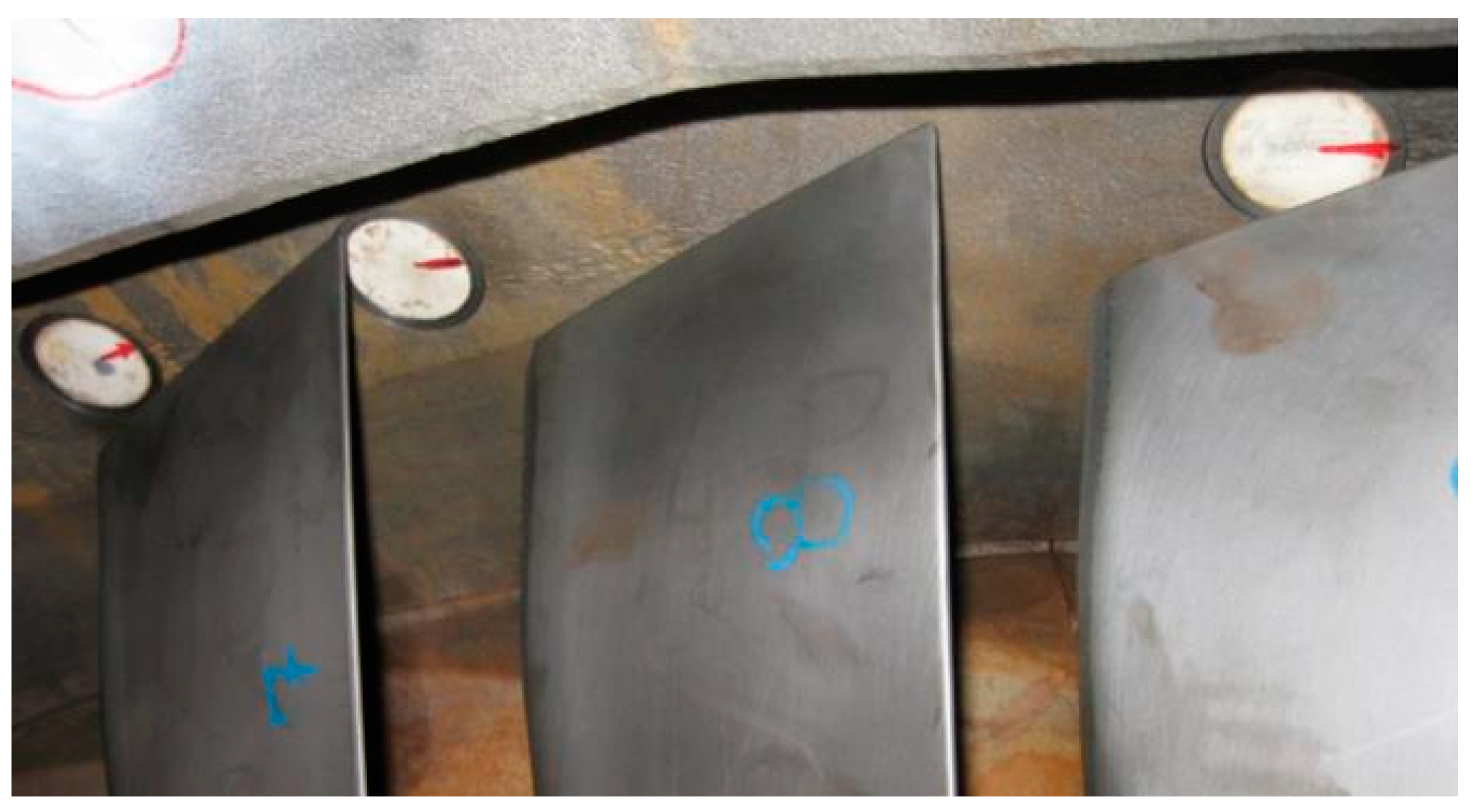
An analysis of 380 MW steam turbine LP last stage rotor blade vibrations in various non-nominal conditions and condenser pressures was carried out.

The rotor blade times of arrival were measured by two inductive sensors installed in the casing at 15 deg. to each other [6,27] (Figure 2).

Test alerts of excessive blade vibration and flutter were provided by an NI CompactRIO controller. The data acquisition system used an NI PXI-1065 computer equipped with PXIe-6358 and PXIe-6612 modules running a LabView application [27]. The time-of-arrival measurements were performed using a 100 MHz clock and 32-bit counters of a PXIe-6612 module, and the TTL pulses were generated by an in-house condition unit [6].

Three measurements were carried out for various condenser pressures and the powers are presented in

Table 1. Blade measurements.

Measurement	Condenser Pressure	Power
1	10.4 kPa–23.6 kPa–11.2 kPa	368.7 MW–365 MW–361.4 MW
2	7.4 kPa–19 kPa–7.4 kPa	299.1 MW–300 MW–298.3 MW
3	5.9 kPa–18.7 kPa–5.9 kPa	219.5 MW–219 MW–218 MW

. In measurement 1, the condenser pressure changed from 10.4 kPa (368.7 MW) to 23.6 kPa (365 MW) and next decreased to 11.2 kPa (361.4 MW). In measurement 2, the condenser pressure was lower than in measurement 1, starting from 7.4 kPa (299.1 MW) to 19 kPa (300 MW) and decreasing to 7.4 kPa (298.3 MW). In measurement 3, the condenser pressure was lower than in measurements 1 and 2, starting from 5.9 kPa (219.5 MW) to 18.7 kPa (219 MW) and decreasing to 5.9 kPa (218 MW).

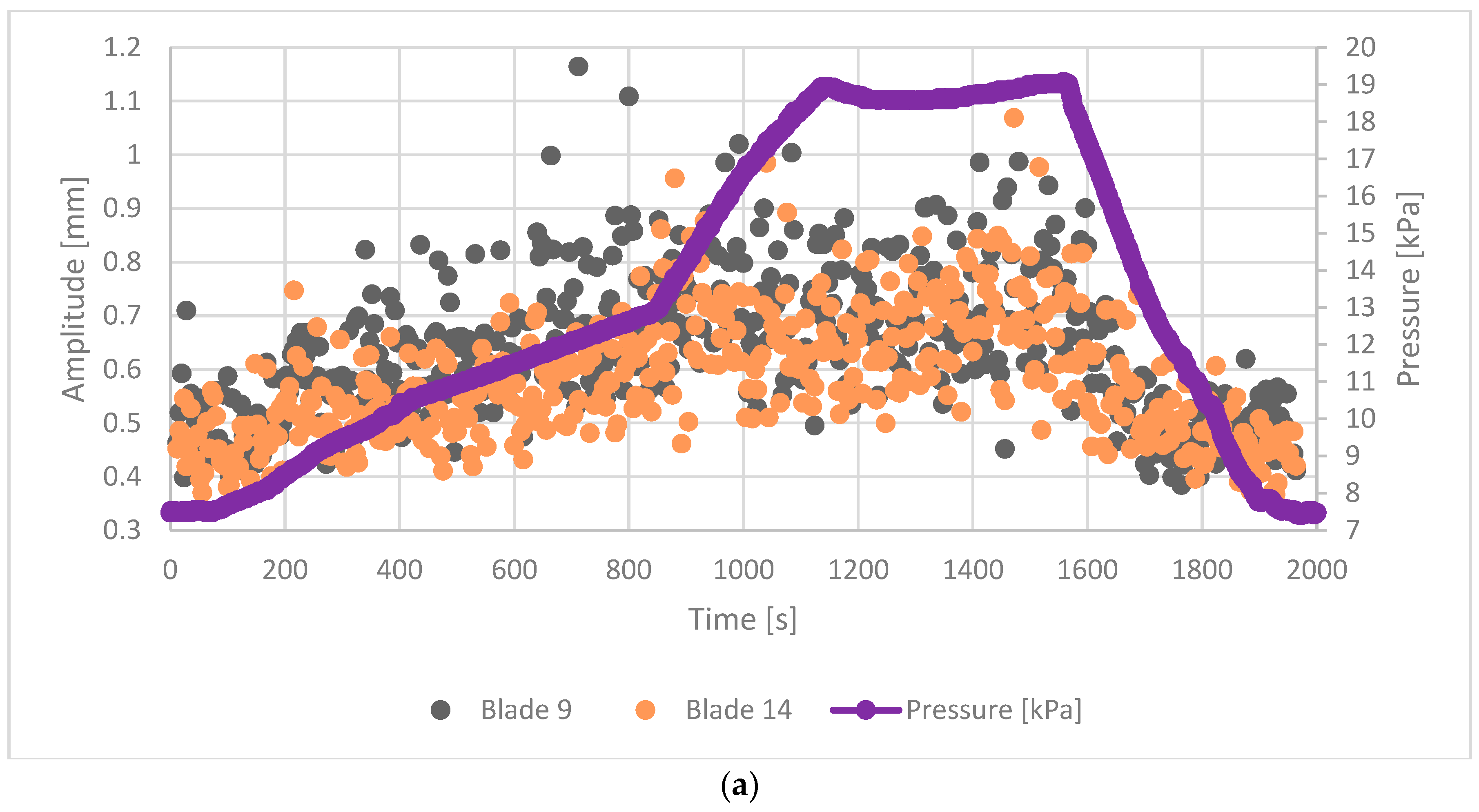
Blade displacements vary with pressure changes in the condenser, increasing with higher condenser pressure and decreasing with lower pressure. By using the nonlinear least squares (L–M) algorithm it is possible to calculate vibration amplitude variations in time for various condenser pressures. Figure 3a shows the amplitudes and condenser pressures (violet line) of blades 9 (green points) and 14 (brownish-red points) in time, for measurement 2. Out of the 53 blades, blade 9 had the highest amplitude and blade 14 had the lowest one. The blade amplitudes in measurement 2 were similar to those of measurement 1. 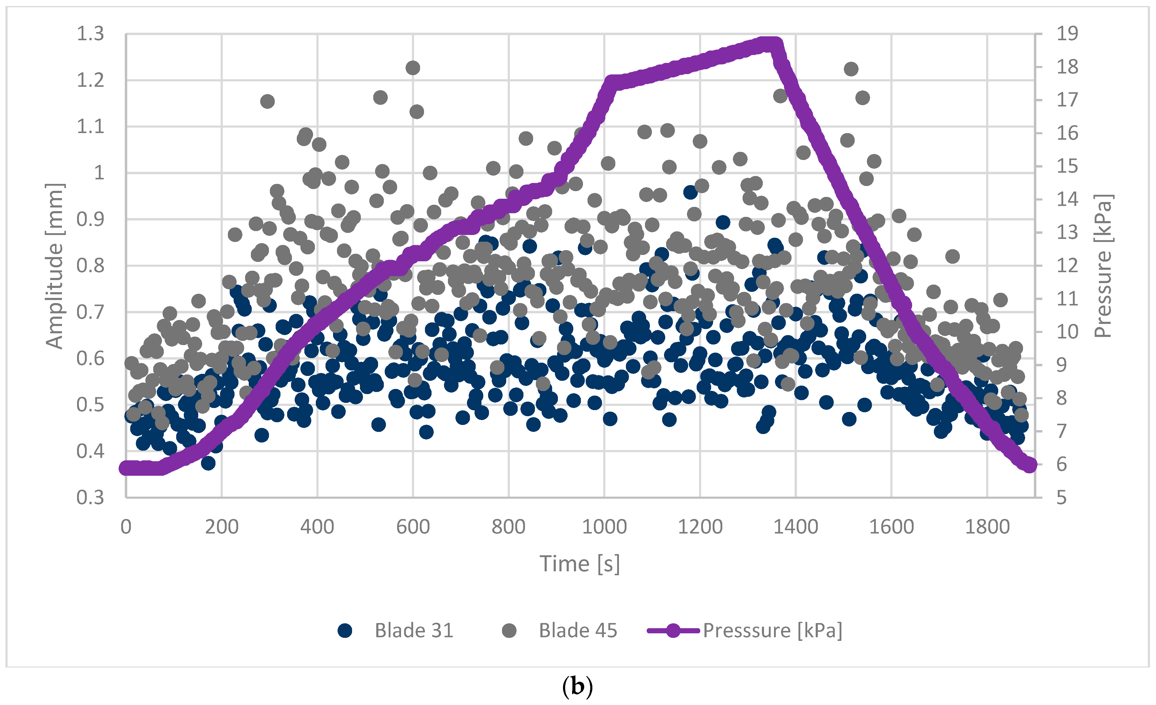Figure 3b shows the amplitudes and condenser pressures of two blades in time, for measurement 3. The green points are the displacements of blade 45, whereas the brownish-red points are the displacements of blade 45. Blade 45 had the highest amplitude and blade 41 had the lowest.

In both cases (Figure 3a,b), the blade amplitudes increased with higher pressure in time.

5. Verification of Tip-Timing Code

In the first step, the L–M tip-timing code is verified using a rotor blade simulator [31].

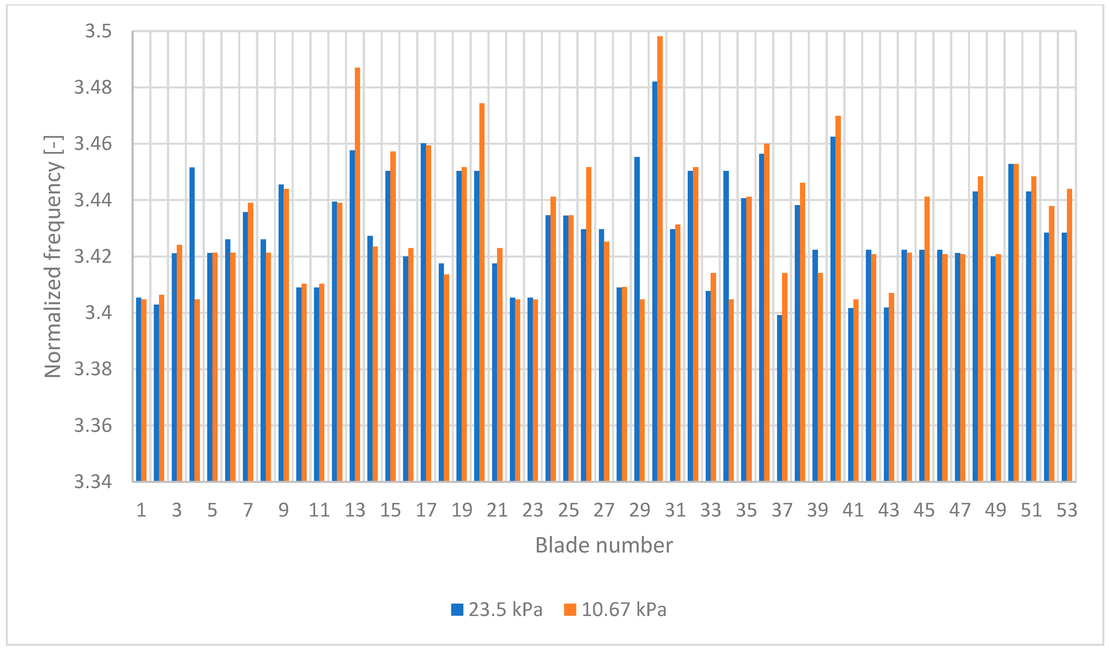
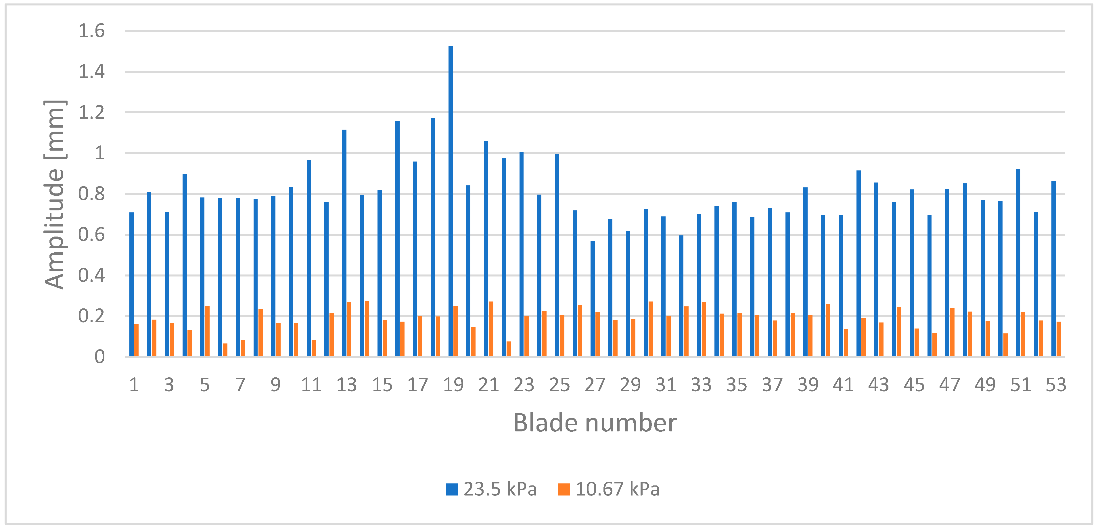
In the next step, the algorithm is verified for nonsynchronous mistuned blade vibrations in a non-nominal regime (Table 1, measurement 1) for condenser pressure at 23.5 kPa (Figure 4) and 10.67 kPa (Figure 5). In mistuned blades, in this case, differences between amplitudes were small. LP last stage mistuned bladed disc nonsynchronous blade vibrations were measured by Przysowa et al. [27].

The obtained rotor blade amplitudes were compared with the nonsynchronous tip timing results in [27] for one-mode blade vibrations. For this purpose, one mode of blade vibration is assumed in the L–M algorithm (Equation (1)). The comparison was satisfactory, with below 10% differences for most blades, Figure 4. The blue bars are the one-mode amplitudes from the L–M algorithm and the red ones are the results from [27].

In the case of lower condenser pressure (10.67 kPa, measurement 1), the differences between blade amplitudes were below 10%, Figure 5. The blue bars are the amplitudes from the L–M algorithm for one mode and the red ones are the results from [27].

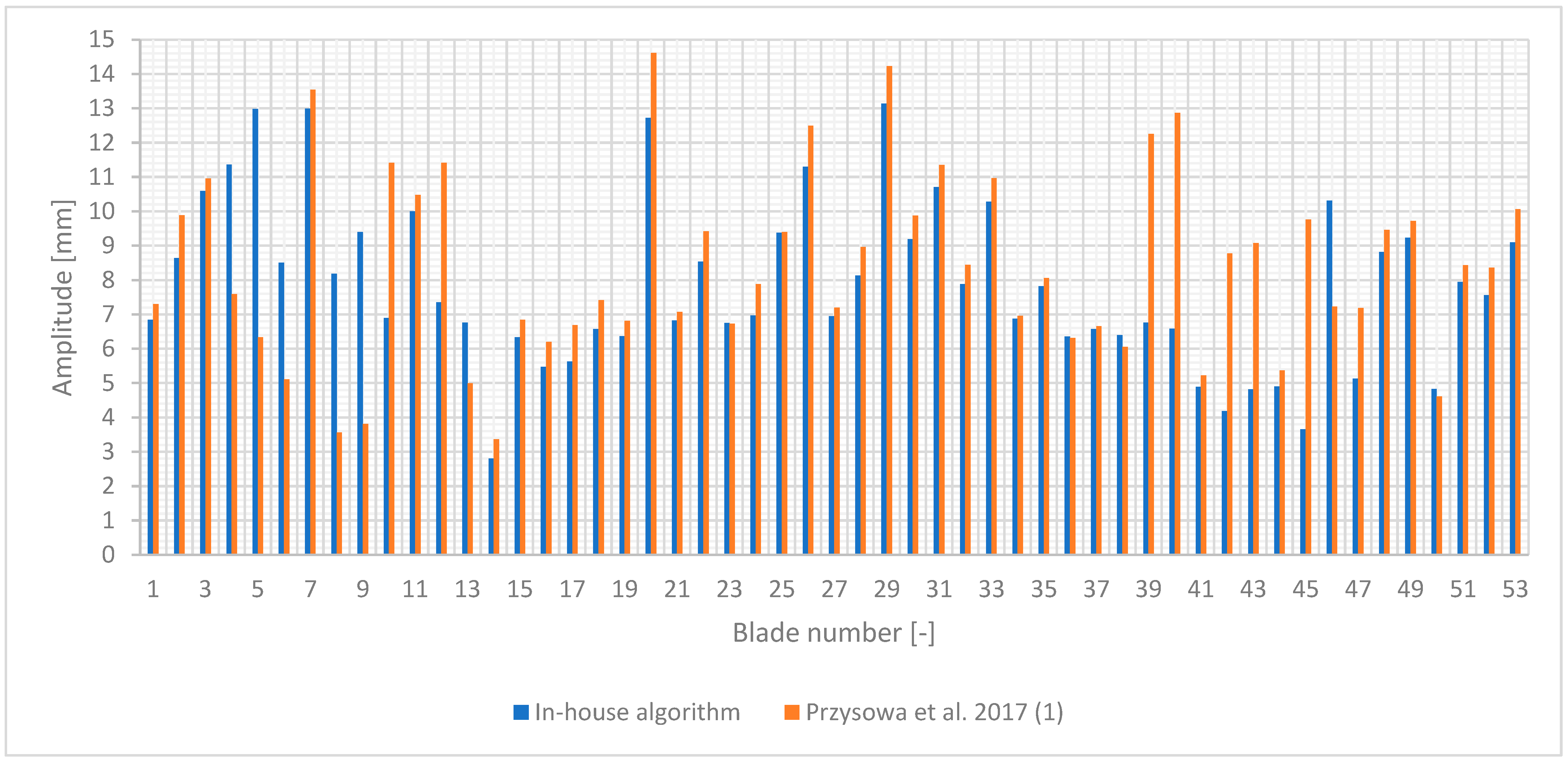
The synchronous blade vibrations of an LP last stage mistuned bladed disc were measured in a vacuum spin chamber during run-down (Przysowa et al. [6,26], Rzadkowski [32]). Single-coil inductive sensors detected blade tip deflections, while every revolution was signaled by a once-per-revolution sensor located between the rotor front support and stage. Fourteen sensors were installed above rotor blades in seven positions (seven pairs of sensors at different axes) [32]. The blades were excited using a manually regulated airflow from a telescopic pipe with a suitably shaped nozzle. The test was carried out during run-down (synchronous vibration). The tip displacements of 53 blades during a reduction of speed from 2028 rpm to 1516 rpm [6,26] were analyzed.

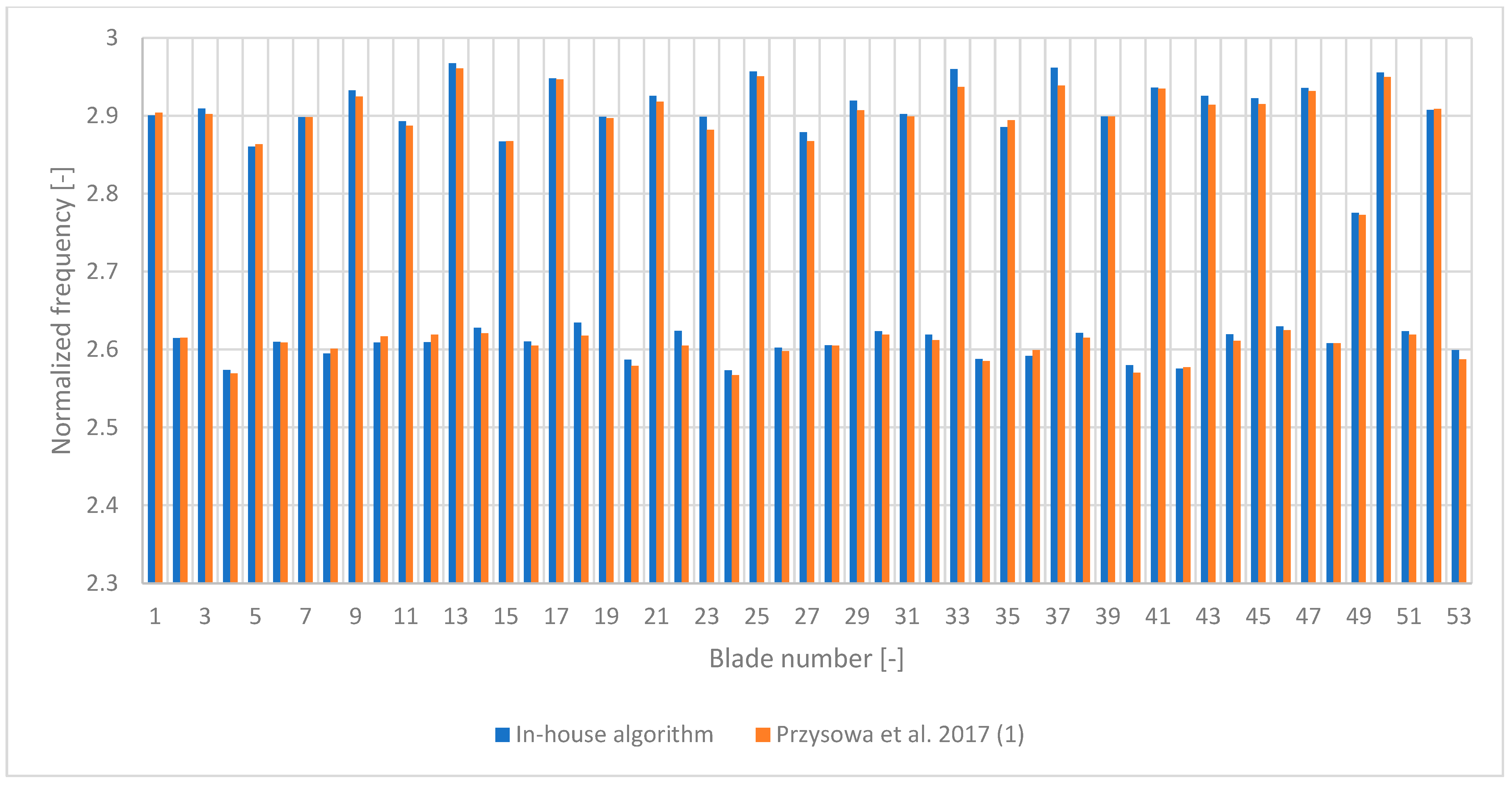
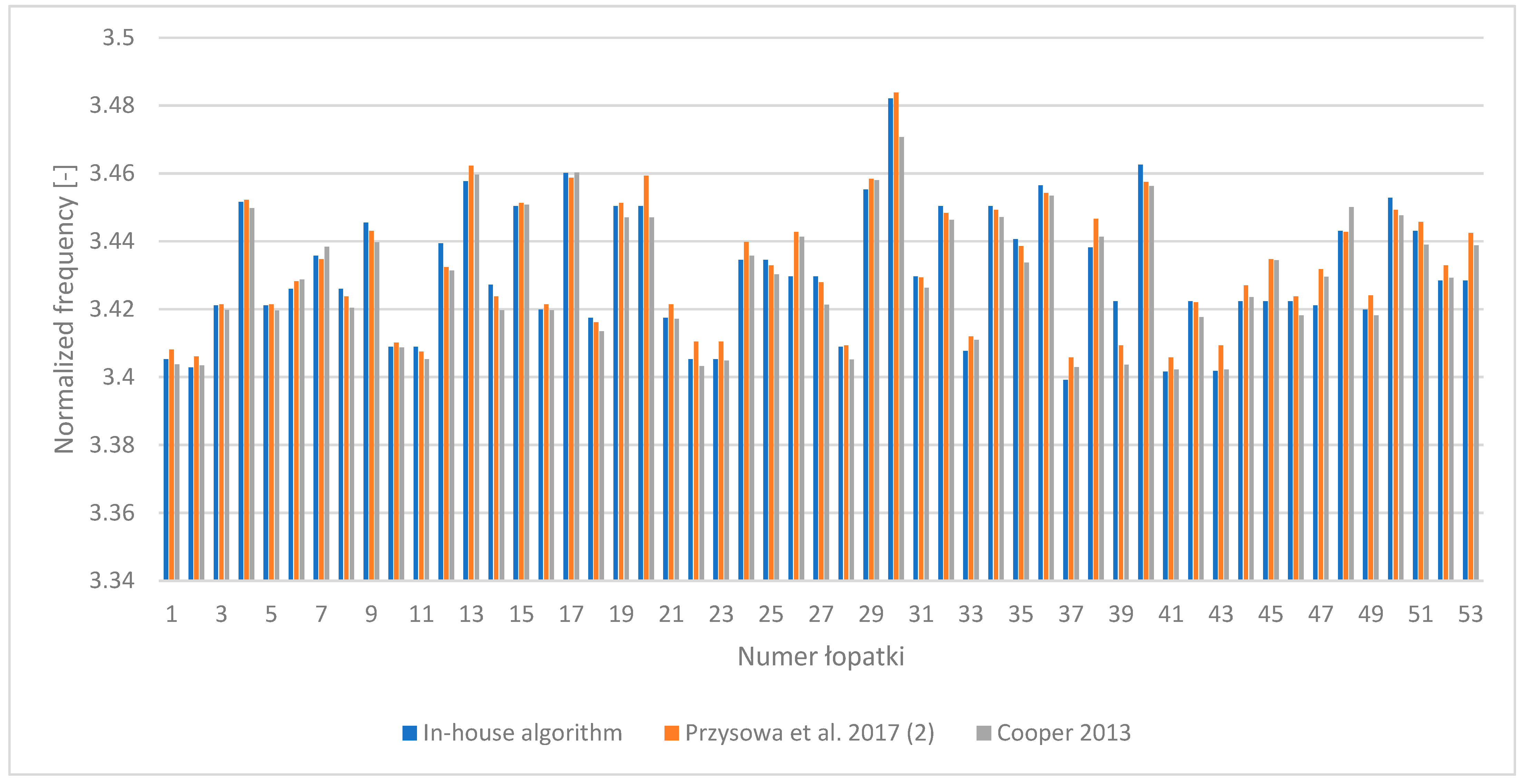
Figure 6 presents the blade amplitudes obtained from the L–M algorithm (blue) and from [26] (red). Figure 7 presents the frequencies. The comparison is satisfactory, with differences below 10% for the majority of the analyzed turbine blades.

6. The Influence of the Number of Sensors on the Accuracy of the Nonlinear Least Squares Levenberg–Marquardt Tip-Timing Fitting Method

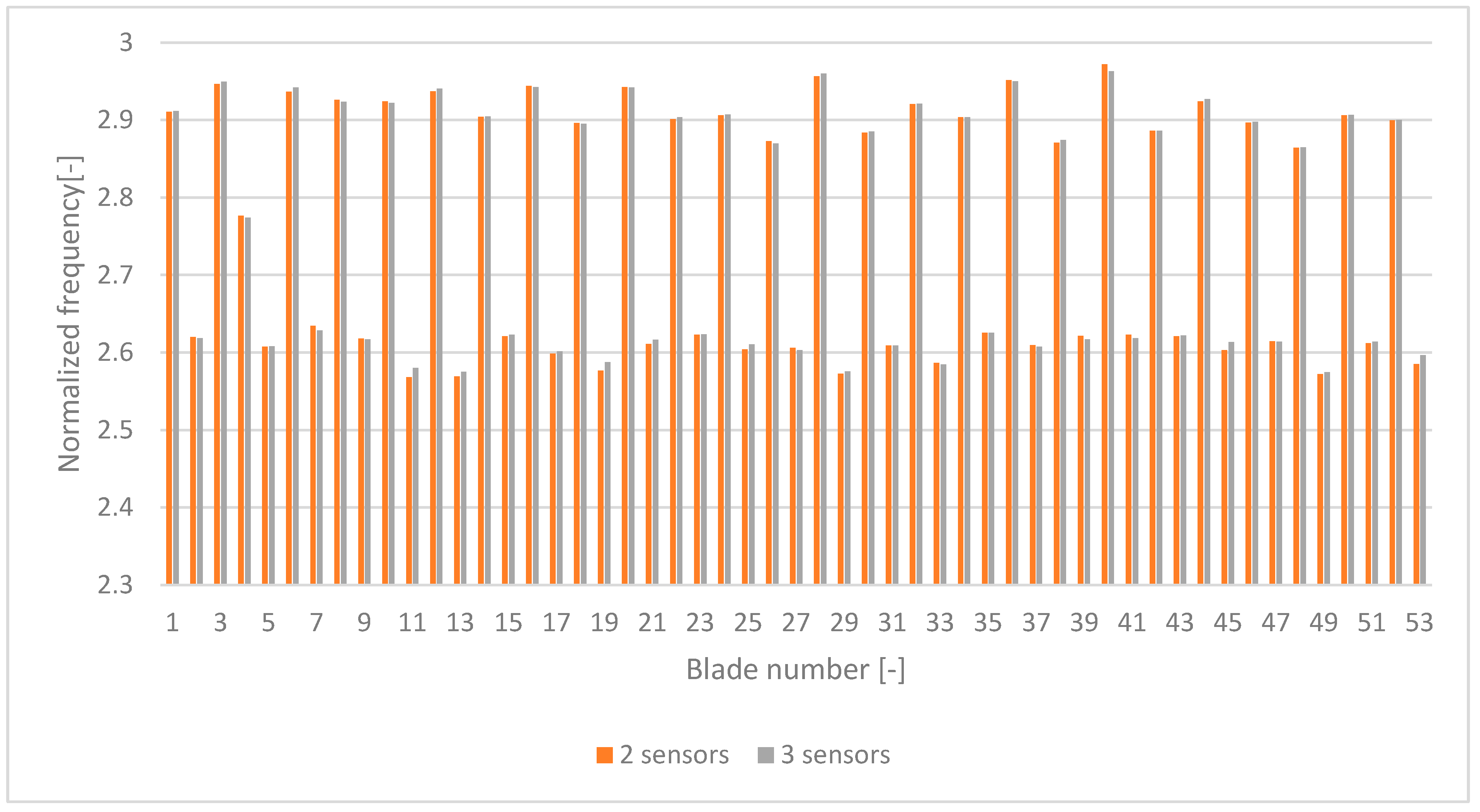
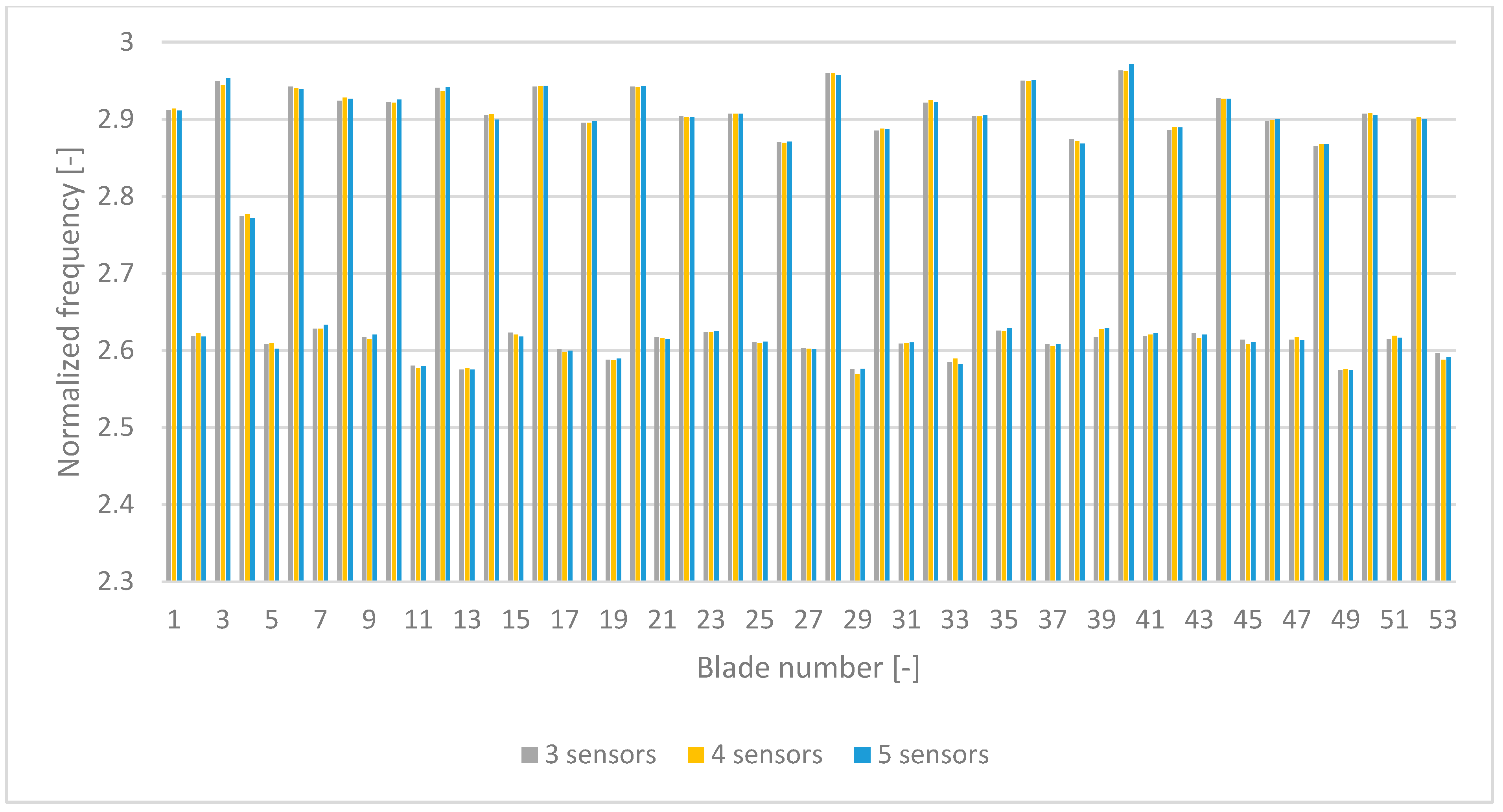
One of the main advantages of the nonlinear least-squares fitting method for tip-timing displacements is the fact that it requires only two sensors to give accurate results. Figure 8 shows that the differences between two sensors and three sensors for synchronous vibrations were below 1%. in normalized frequencies. Rotor blade normalized frequencies for 3, 4 and 5 sensors varied no more than 0.4% (Figure 9).

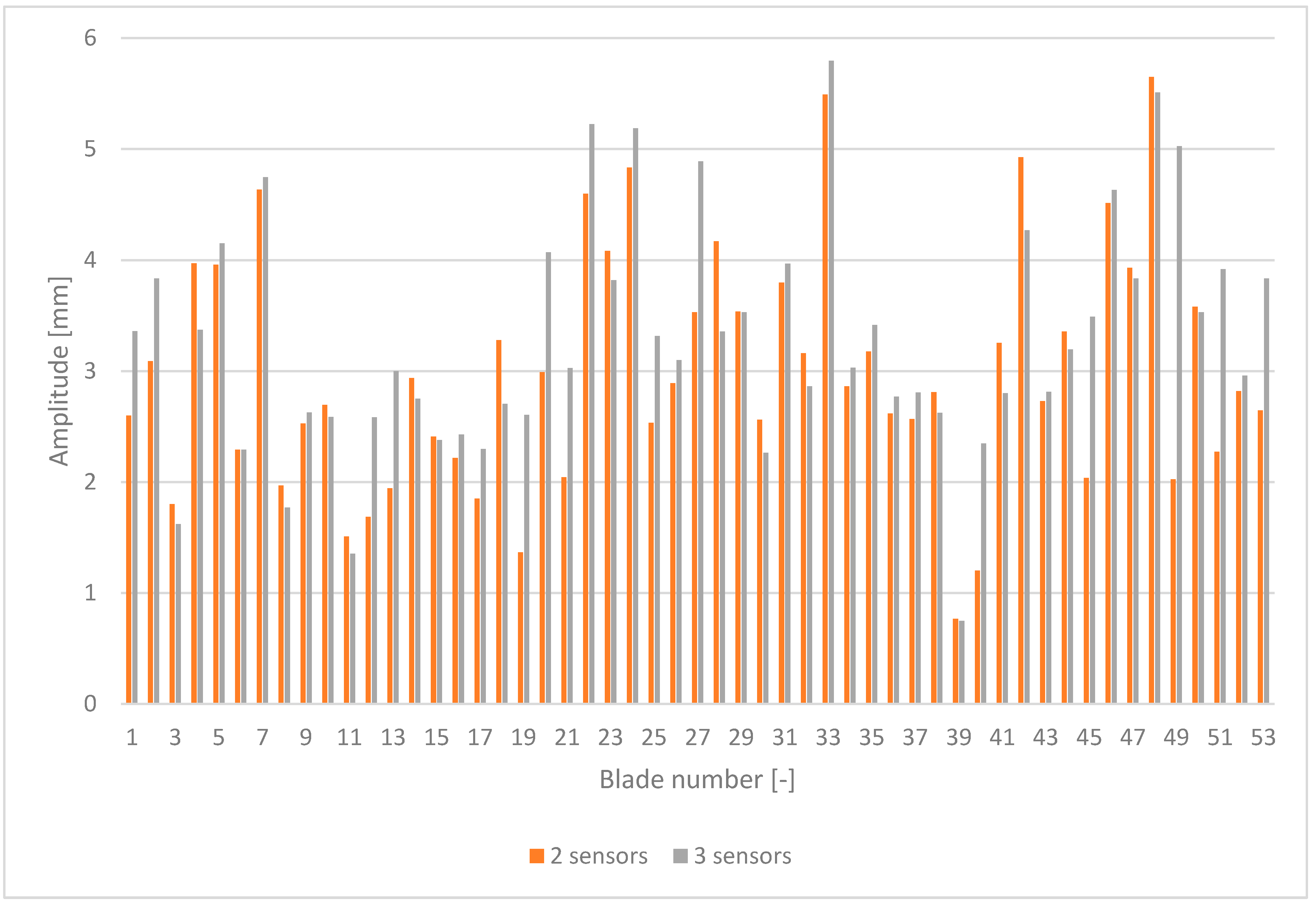
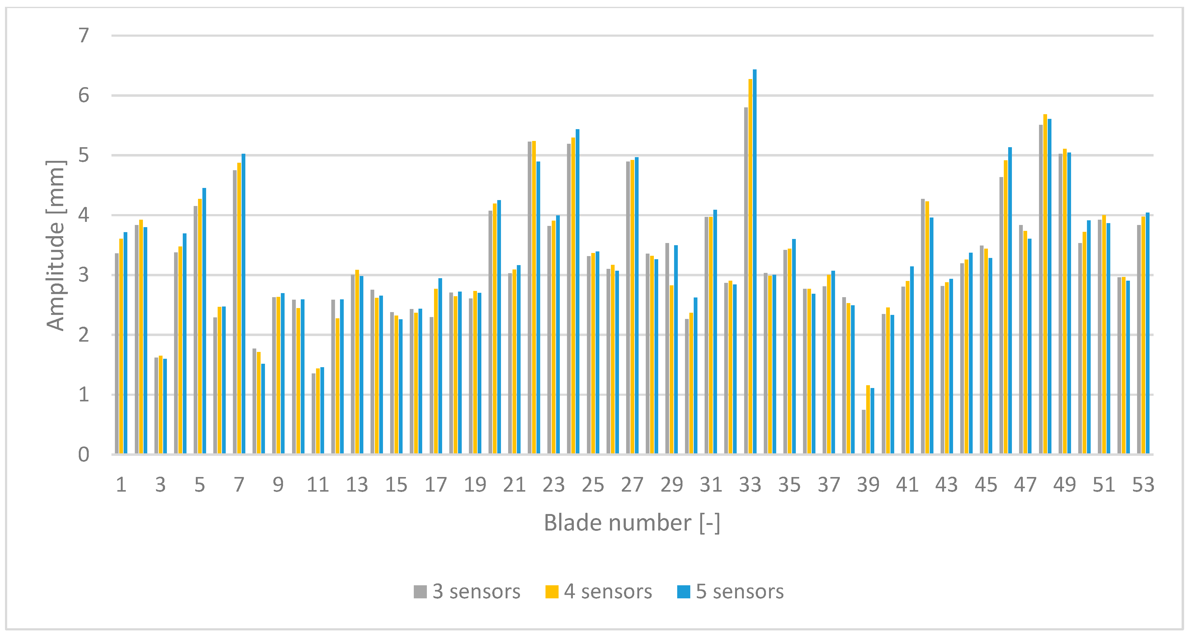
For rotor blades amplitudes, the differences between two sensors and three sensors were around 10% (Figure 10). When the number of sensors was increased to four and then to five (Figure 11), the differences between amplitudes for three, four and five sensors were around 1–2%.

The influence of the number of sensors on the accuracy of obtaining blade amplitude and frequency have been analyzed. However, the accuracy of the L–M method in comparison to one-mode analysis will be presented in the last section.

7. Rotor Blade Amplitude for Non-Nominal Conditions

Presented here are the blade amplitudes for non-nominal conditions with various condenser pressures and powers.

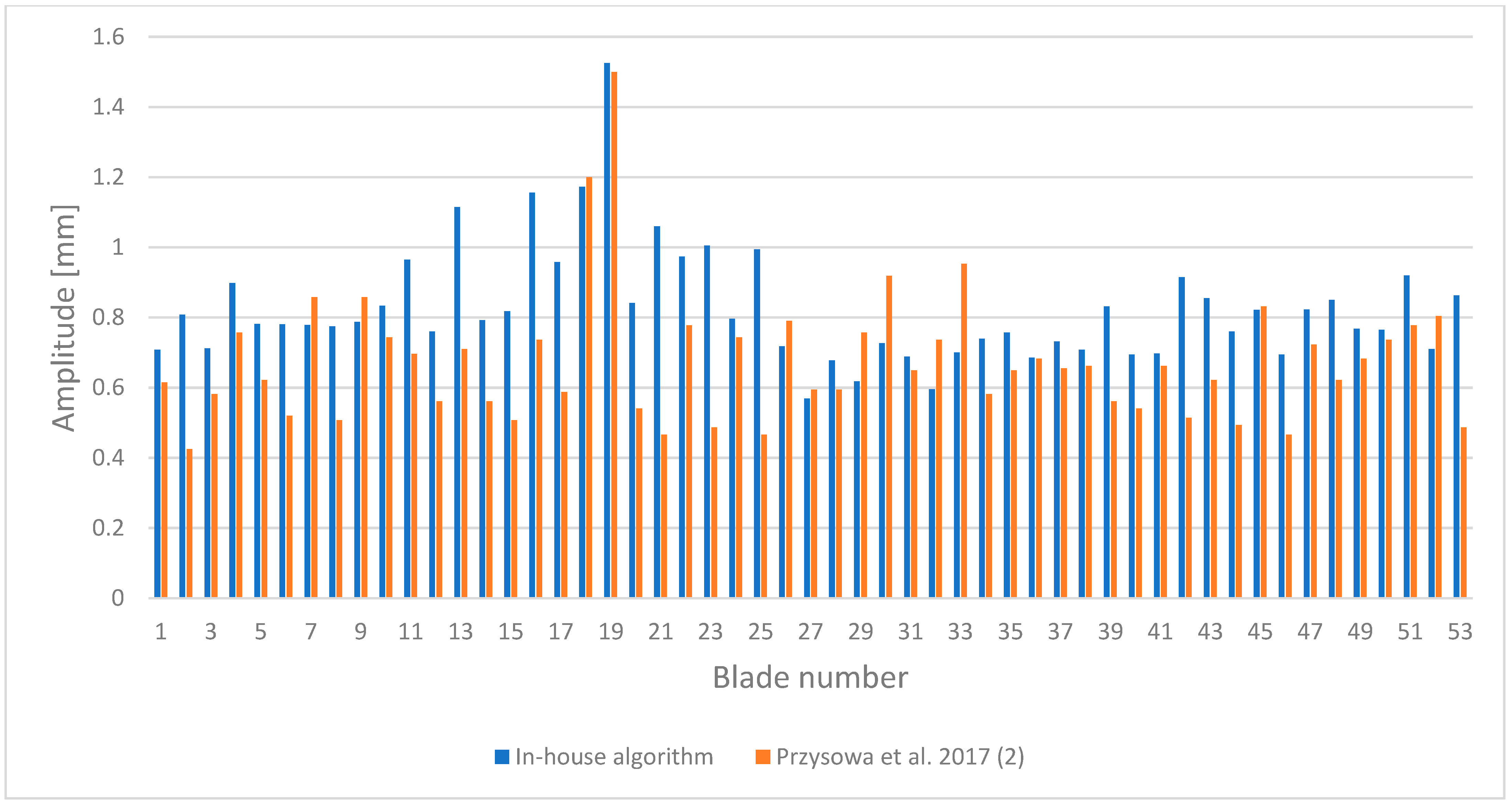
Figure 12 presents a comparison of all the blade amplitudes in measurement 1 for pressures 23.5 kPa and 10.67 kPa. This shows that blade amplitude increased in proportion to condenser pressure.

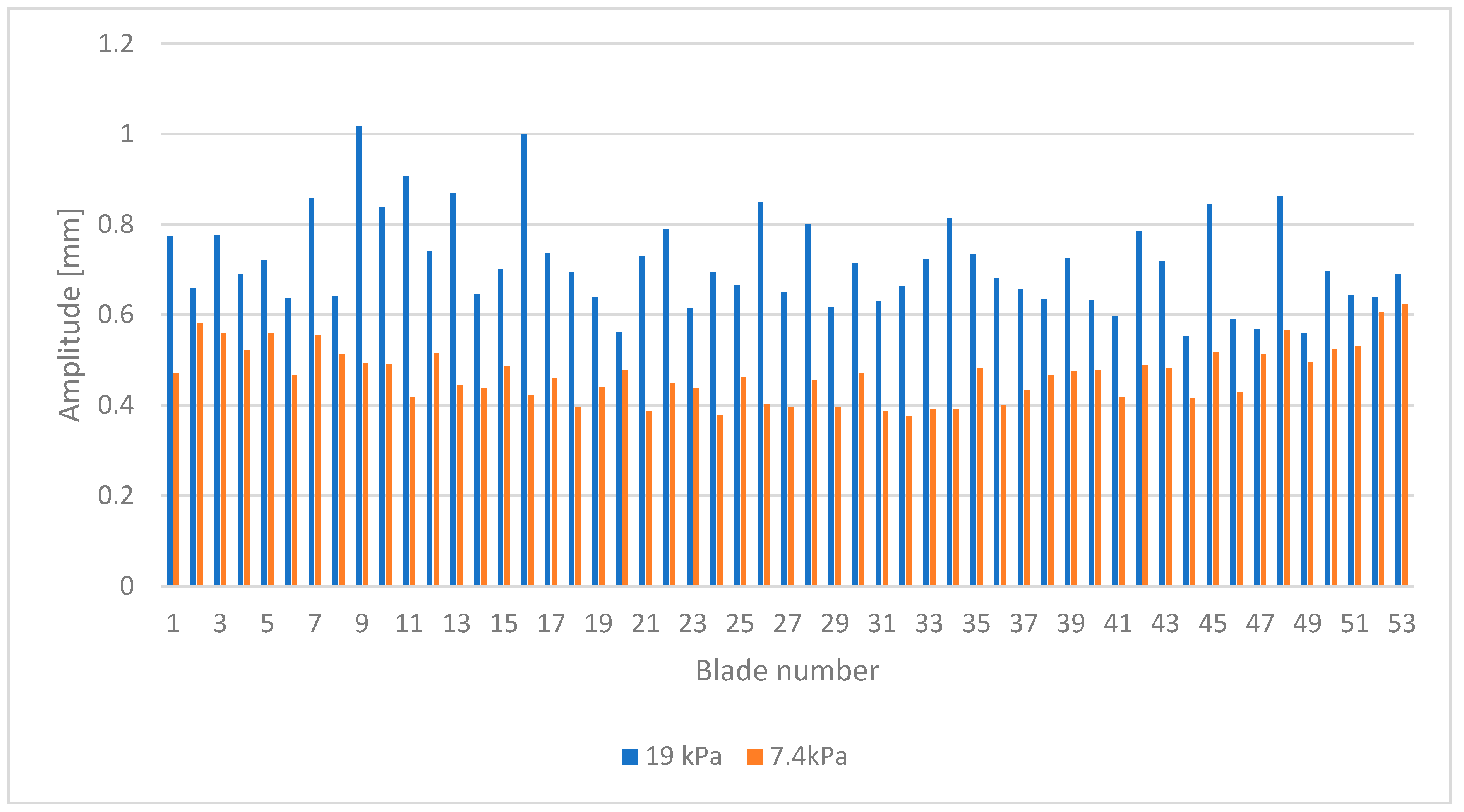
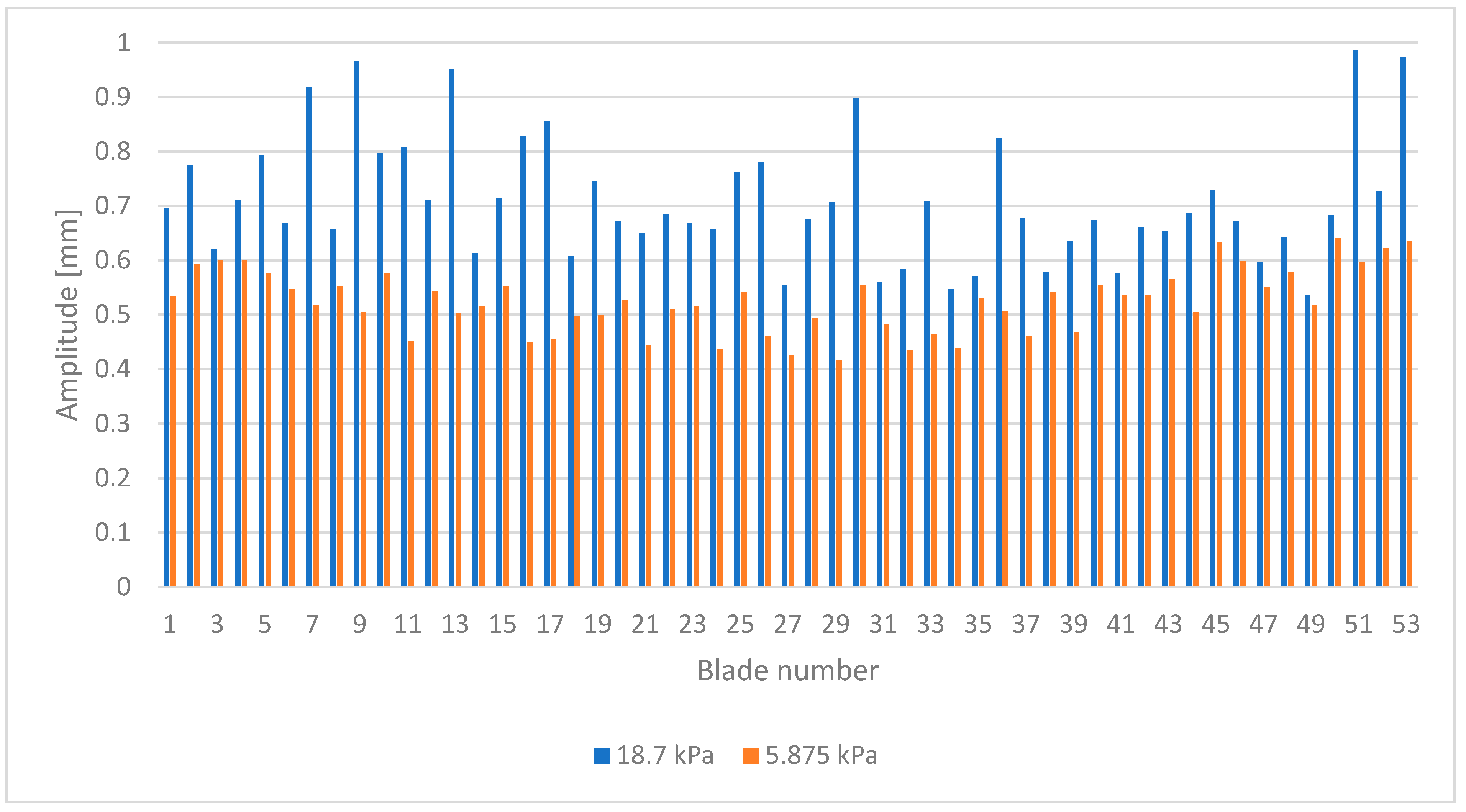
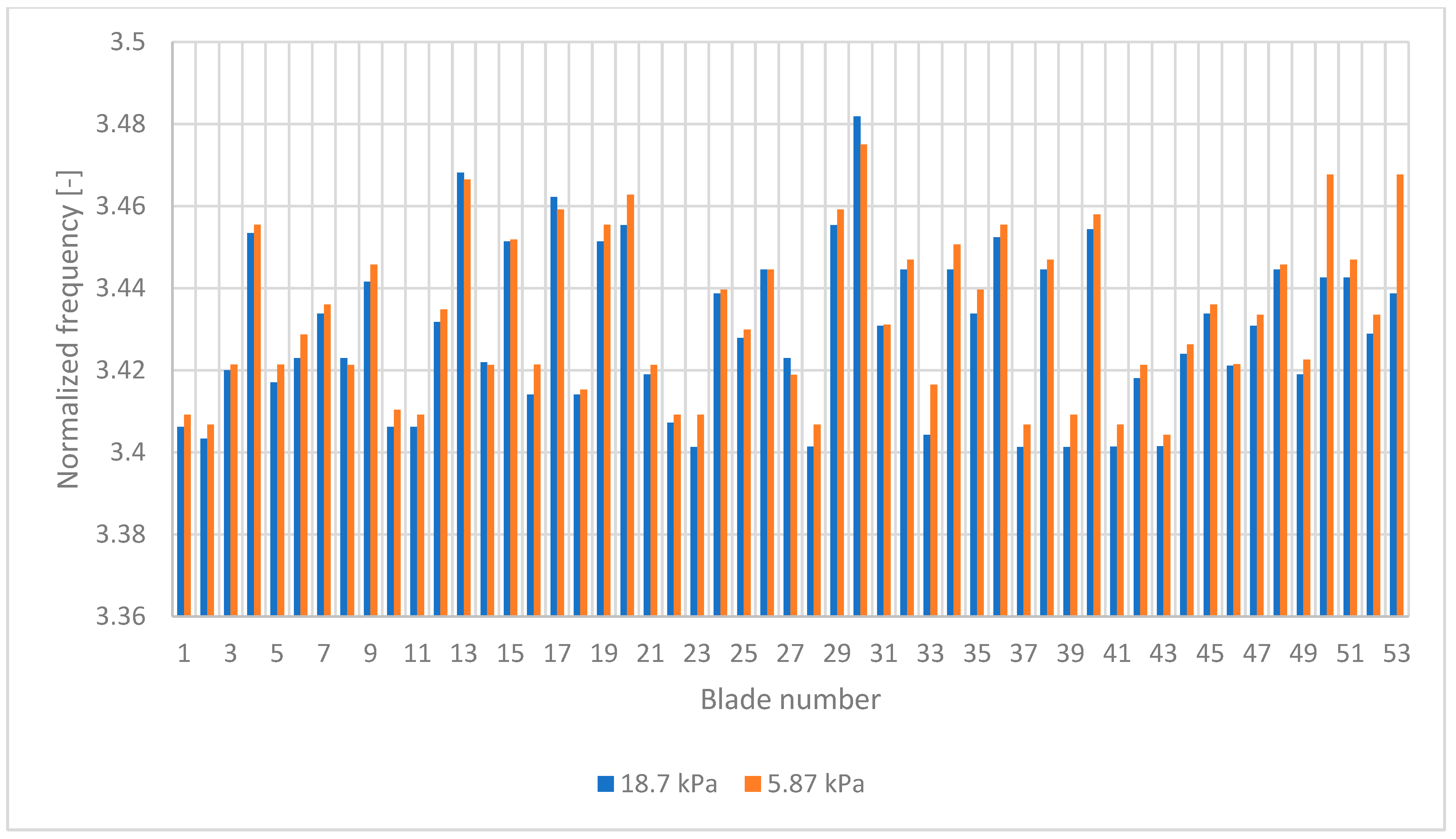
Figure 13 and Figure 14 show a comparison between amplitudes in low and high condenser pressures for measurements 2 and 3.

The highest amplitudes, up to 1.58 mm, occurred with 23.5 kPa at 365 MW (Figure 12) and decreased to 1.02 mm as the pressure decreased to 19 kPa at 300 MW (Figure 13) and to 0.99 mm for 18.7 kPa at 219 MW (Figure 14).

For measurements 2 and 3, the amplitude for higher pressure was larger than for lower pressure, although the difference was not as large as in the case of measurement 1. This is because the unsteadiness of the blade forces was higher for measurements 2 and 3 [33].

8. Rotor Blades Frequencies for Non-Nominal Conditions

For the highest and lowest condenser pressures in measurement 1, the frequencies were obtained and compared with [27,28].

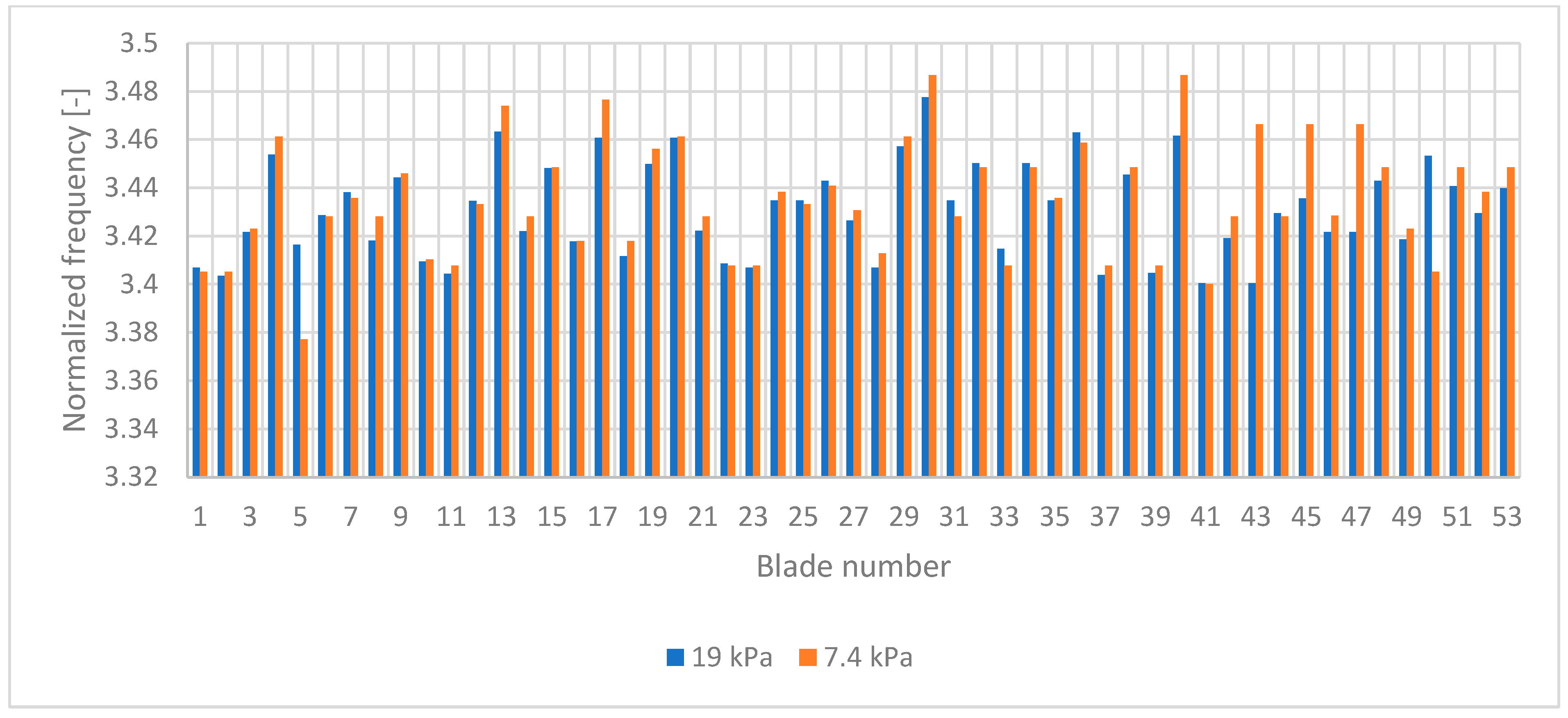
The differences between the L–M and [27,28] frequencies were below 1% (Figure 15) because one mode in fitting was assumed in the L–M and [27,28]. The amplitudes were compared in Figure 4.

The blade frequencies for measurements 2 and 3 were similar to those of measurement 1 (Figure 16, Figure 17 and Figure 18).

The results show that the higher condenser pressure increased blade amplitudes, but they did not increase their frequencies.

In [27], blade vibrations were analyzed for condenser pressures ranging from 10.4 to 23.6 kPa (368.7–365 MW). In this paper, blade vibrations were analyzed with condenser pressure ranging from 7.4 to 19 kPa (299.1–300 MW) and from 5.9 to 18.7 kPa (219.5–219 MW). This covers the entire non-nominal work range of a 380 MW steam turbine LP last stage, which is a novelty in the literature.

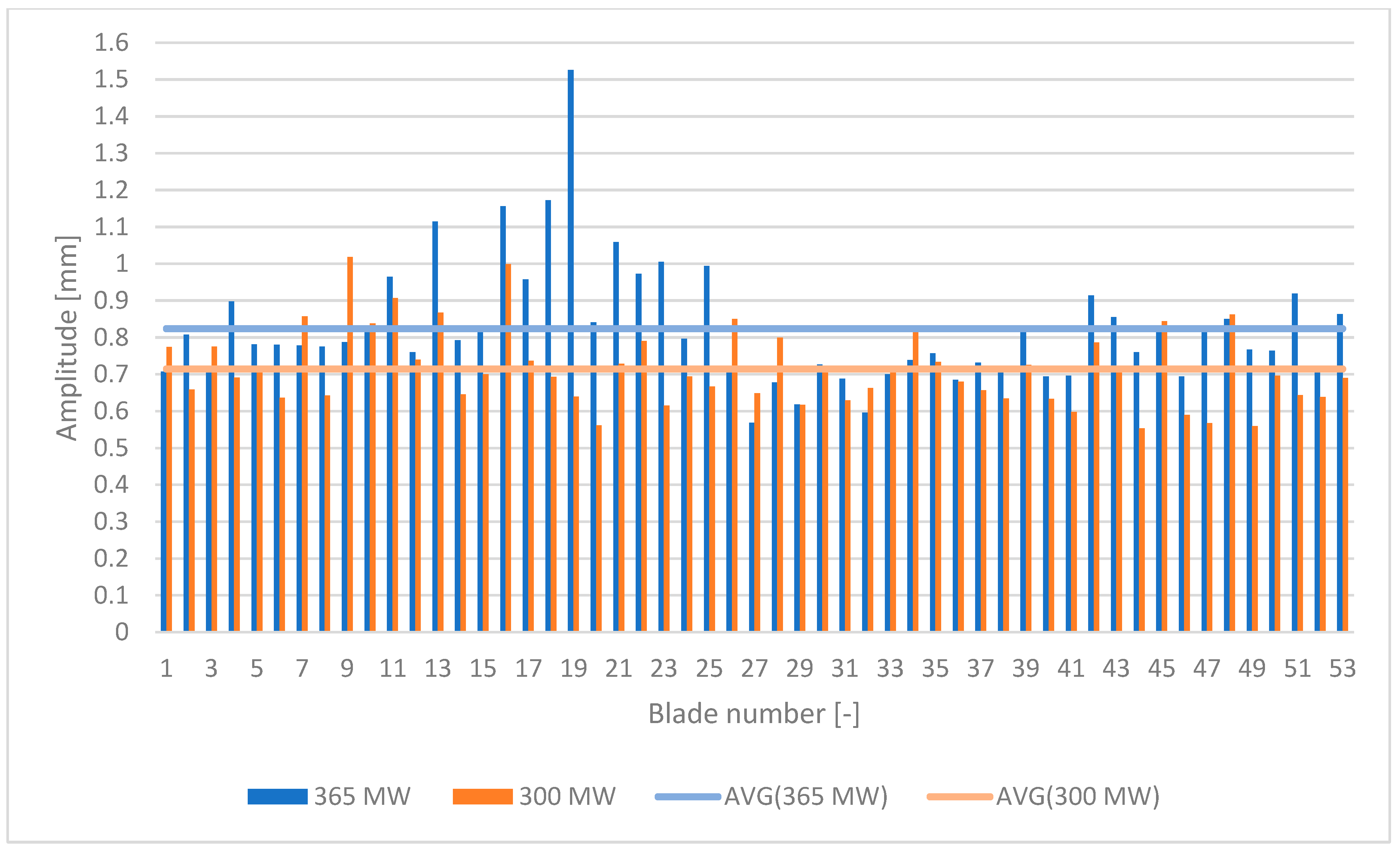
Figure 19 and Figure 20 present the rotor blade amplitudes for various turbine powers. The maximal blade amplitude for 365 MW was 1.56 mm, whereas for 300 MW it was 1.03 mm. The average blade amplitude was 0.81 mm for AVG (365 MW) (Figure 19) and 0.72 mm for AVG (300 MW) (Figure 20). This shows that for 365 MW (Figure 19), the average rotor blade amplitudes were higher than for 300 MW.

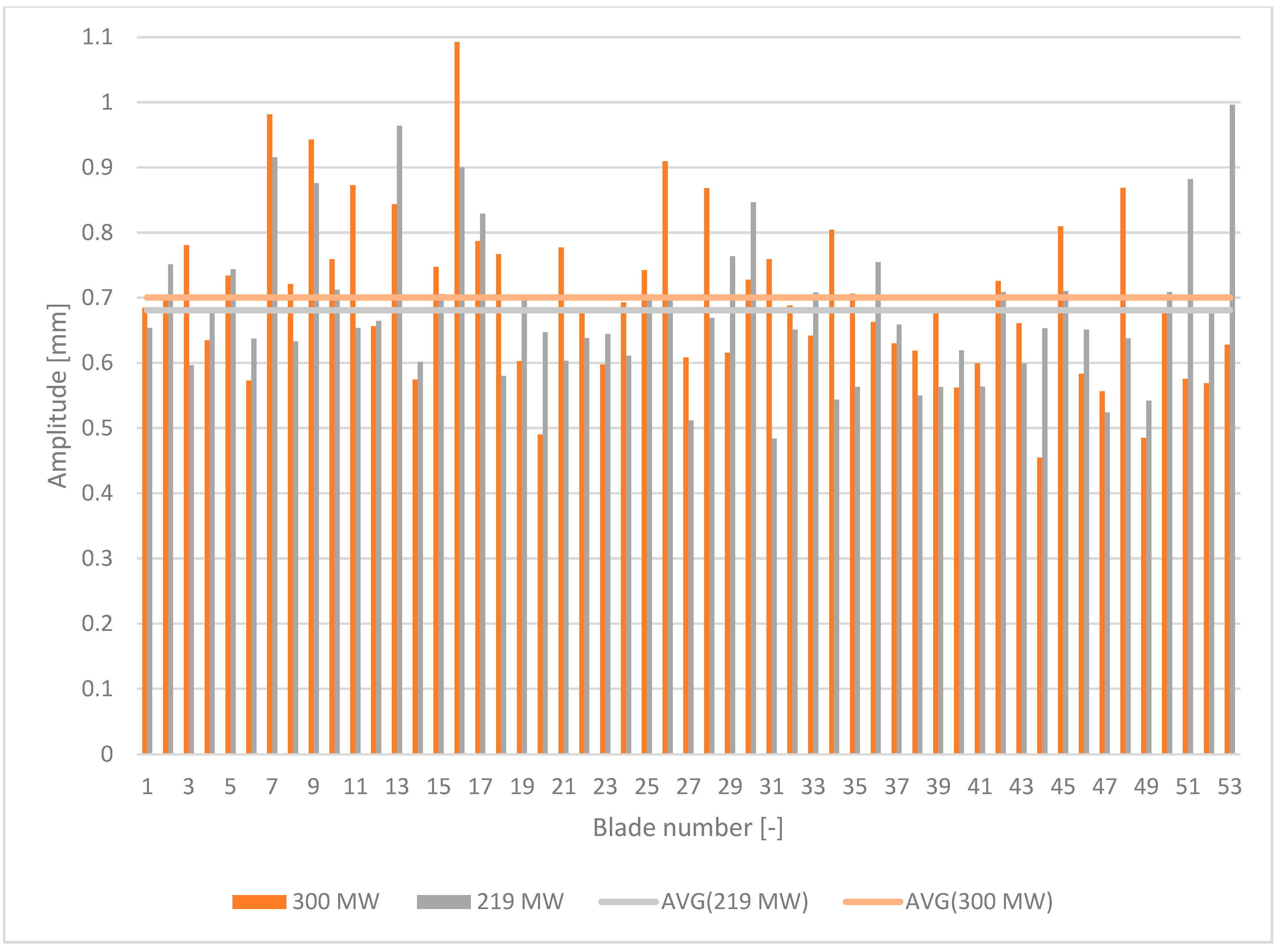
Figure 20 shows that the rotor blade amplitude was higher at 300 than at 219 MW. The maximal blade amplitude for 300 MW was 1.09 mm, whereas it was 0.98 mm for 219 MW. The average blade amplitude for 300 MW was 0.7 mm (AVG (300 MW), Figure 20), and 0.68 mm for 219 MW (AVG(219 MW) (Figure 20).

The rotor blade displacement was also higher for higher turbine powers, although this dependence was nonlinear.

9. Multimode Analysis for Non-Nominal Conditions

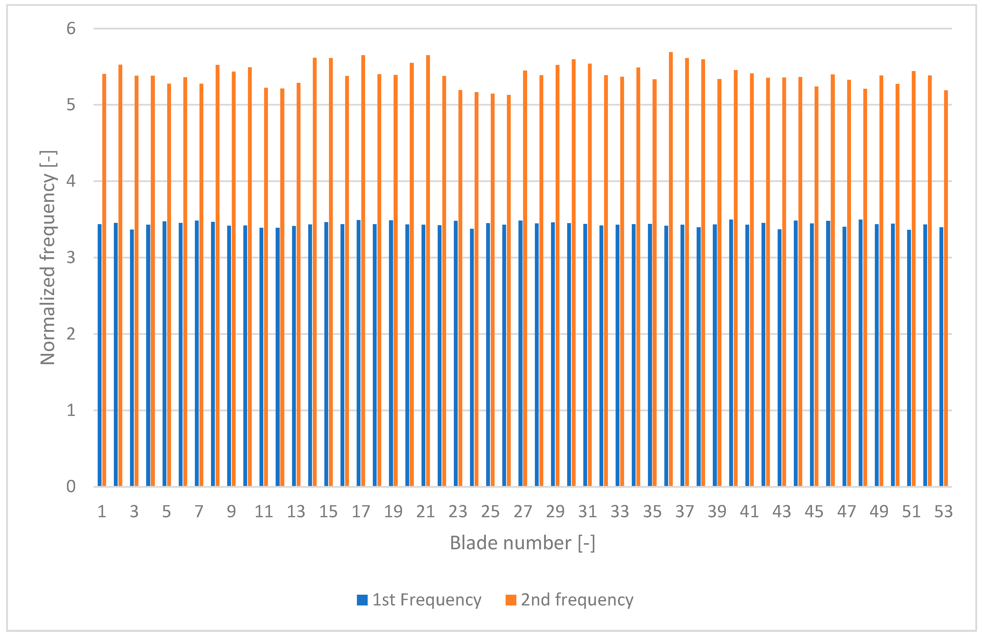
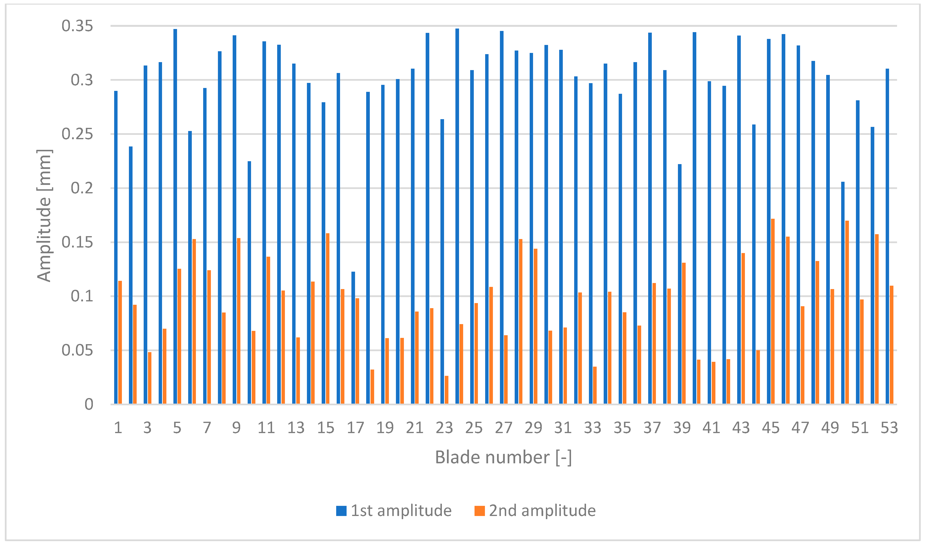
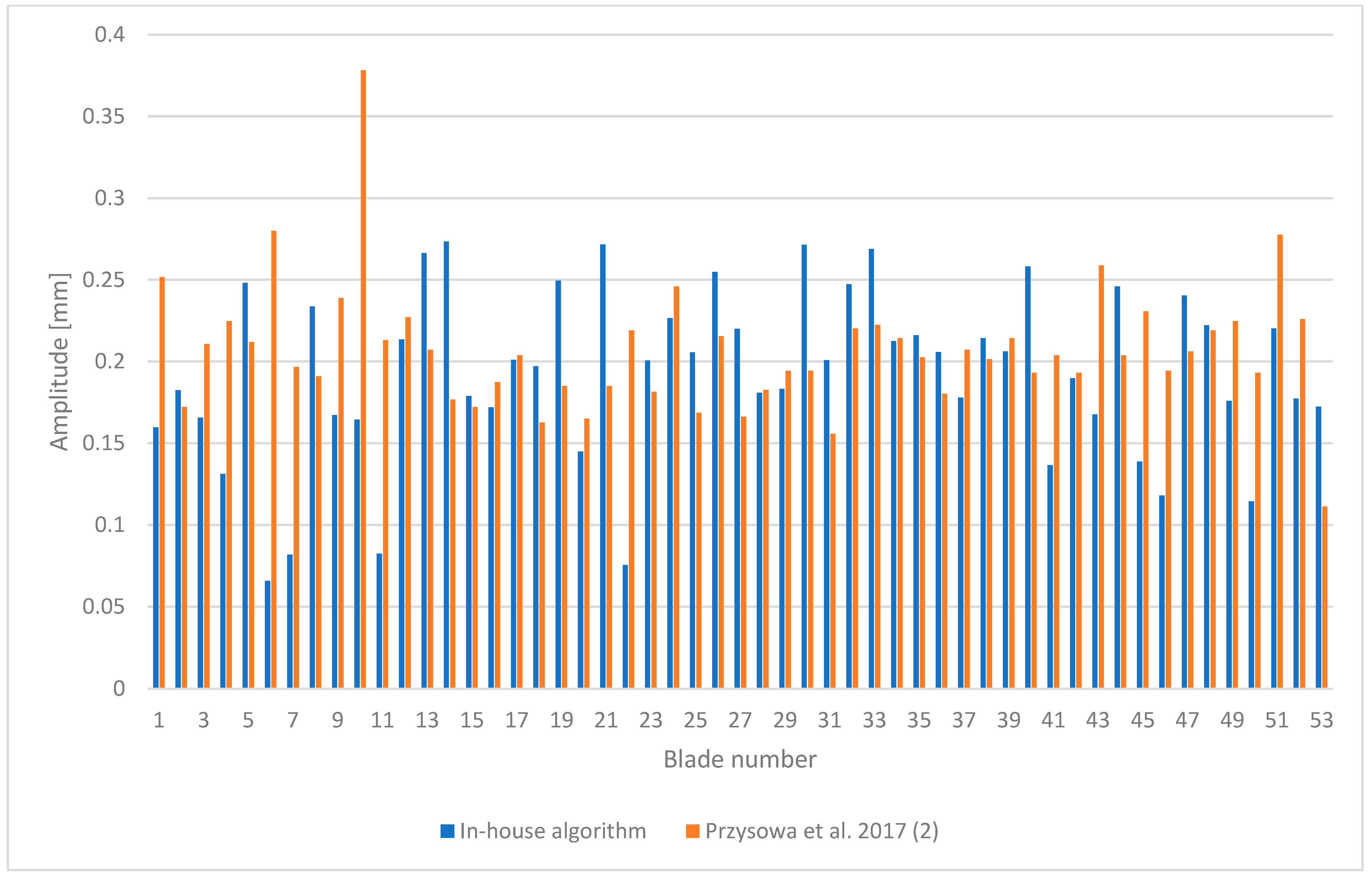
The L–M algorithm was used for a multimode analysis (Equation (3)) of rotor blades in measurements 1, 2 and 3. This showed that all the blades vibrated in the 1st and 2nd mode simultaneously, which is a novelty. Figure 21 and Figure 22 present 1st and 2nd mode blade amplitudes and frequencies for measurement 1. The blade frequency results were similar for all three measurements. The figures show that the 2nd mode of vibration frequency appeared at about 3.5 [-], which corresponds to the second blade natural frequency. The 3rd mode did not appear.

The 2nd blade mode amplitude was significantly lower than the 1st blade mode amplitude.

The maximum 1st mode blade amplitude was about 0.349 mm and 0.17 mm for the 2nd mode for condenser pressure 23.5 kPa in measurement 1 (Figure 22).

The 1st blade amplitude for the 1st mode was about 0.31 mm and 0.11 mm for the 2nd mode for condenser pressure 23.5 kPa in measurement 1 (

Table 2. Comparison between fitting results obtained from methods 1 and 2 for blade 1, condenser pressure 23.5 kPa (Measurement 1).

Result	Method 1	Method 2
1st frequency	3.394	3.412
1st amplitude	0.31 mm	0.211 mm
2nd frequency	5.191	5.273
2nd amplitude	0.11 mm	0.038 mm

).

For measurement 2 and condenser pressure 19kPa (

Table 3. Comparison between fitting results obtained from methods 1 and 2 for blade 1, condenser pressure 19 kPa (Measurement 2).

Result	Method 1	Method 2
1st frequency	3.371	3.412
1st amplitude	0.22 mm	0.206 mm
2nd frequency	5.642	5.306
2nd amplitude	0.044 mm	0.069 mm

), the 1st blade amplitude of the 2nd mode was lower than for measurement 1 (Table 2).

The above multimode analysis results were compared with the results in [34], which presented the method of finding one-mode synchronous and nonsynchronous blade vibrations from the tip-timing velocity time of arrival using the least squares technique. In [34], two sensors were required in the casing without a once-per-revolution sensor and without measuring the rotor blade velocity. The rotor blade velocity was obtained from the measured time of rotor blade arrival and used in the functional of the least squares technique.

In this paper, the above model was altered for a multimode analysis, which is a novelty.

Table 2, Table 3 and

Table 4. Comparison between fitting results obtained from methods 1 and 2 for blade 1, condenser pressure 18.7 kPa (Measurement 3).

Result	Method 1	Method 2
1st frequency	3.418	3.421
1st amplitude	0.343 mm	0.180 mm
2nd frequency	5.591	5.248
2nd amplitude	0.165 mm	0.068 mm

present the amplitudes and frequencies (measurements 1, 2 and 3, respectively) for the L–M algorithm (method 1) and the multimode analysis based on [34] (method 2). For measurement 1 (Table 2), the 1st mode frequency was nearly identical (<1%), although the frequency obtained by method 2 was slightly higher. The amplitude was higher for the 1st blade mode than for the 2nd blade mode, and here there was also a greater disparity between methods 2 and 1. Similar conclusions may be drawn for the 1st amplitude mode in measurements 2 (Table 3) and 3 (Table 4). For the 2nd mode, the frequencies and amplitudes in method 1 were slightly higher.

The general conclusion is that in method 1, the results were similar to those of method 2.

The influence of the number of sensors on blade amplitude and frequency calculation accuracy was analyzed in the previous section.

As already demonstrated, the L–M algorithm can analyze multimode blade vibrations. Such calculations increase the accuracy of amplitude calculations. Figure 21 and Figure 22 show that the blades vibrated simultaneously with two modes in non-nominal regimes. A comparison between a one-mode blade vibration algorithm [27] and the L–M multimode algorithm shows that the blade vibration amplitude for the one-mode algorithm was higher (Figure 23). The one-mode analysis is an approximation of displacements comprising a few modes, which is not precise.

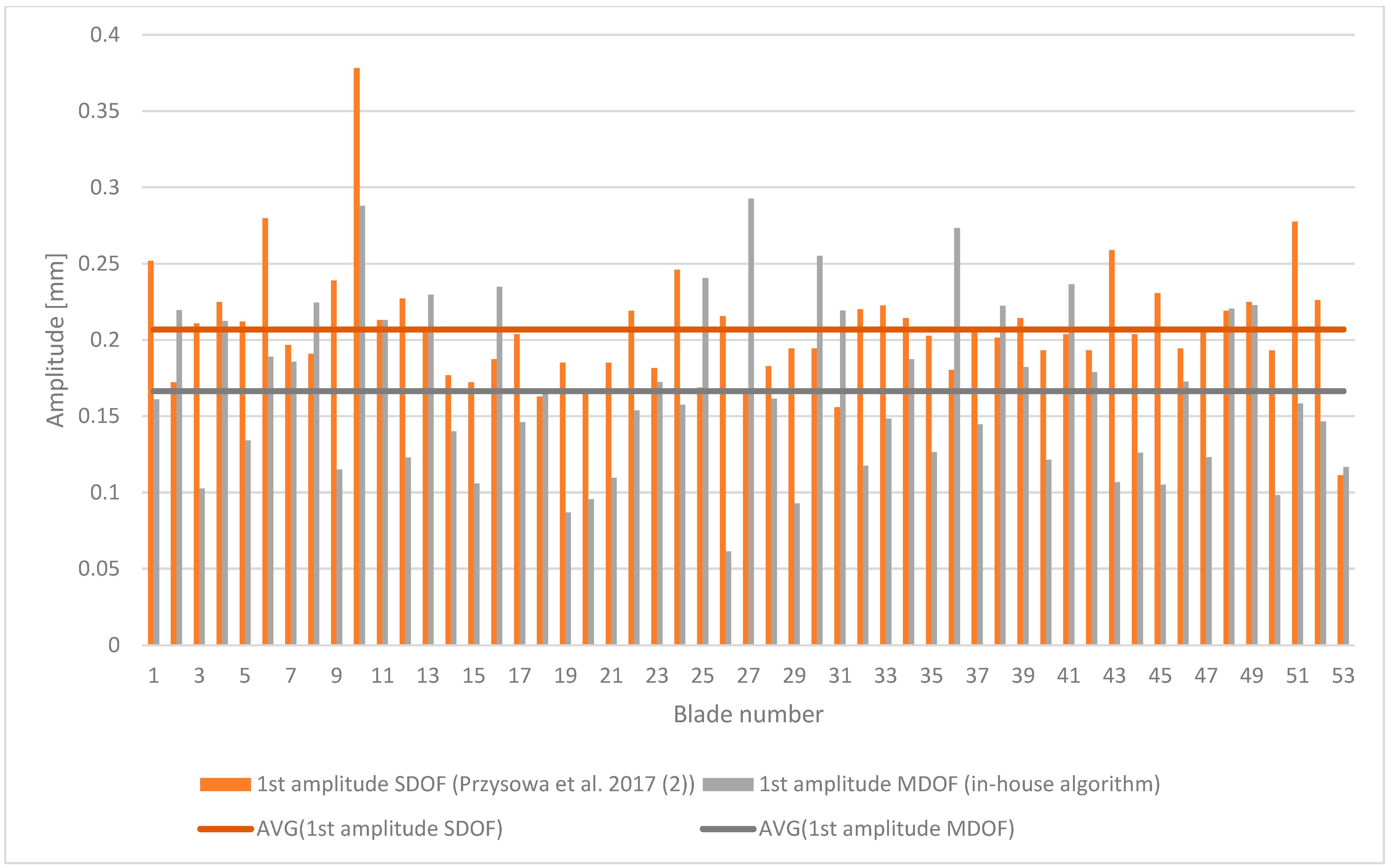
Figure 22 presents the blade amplitude for 53 blades (measurement 1) with 10.67 kPa condenser pressure. The one-mode (SDOF) [27] blade amplitudes are red and the multimode (MDOF) 1st mode amplitudes are green. The horizontal red line is the averaged SDOF blade amplitude [27] and the horizontal green line is the averaged multimode (MDOF) 1st mode blade amplitude. This clearly shows that the one-mode averaged blade amplitude was 29% higher than that of the multimode 1st mode. This is an estimation of the accuracy of the L–M algorithm for multimode blade vibrations. Its accuracy in calculating blade vibration amplitudes could be very important from the point of view of blade life. The procedure of life calculation is presented in [35].

10. Conclusions

This paper presented the use of a nonlinear least squares Levenberg–Marquardt algorithm to measure nonsynchronous rotor blade vibrations in the LP the last stage of a 380 MW steam turbine with various condenser pressures in non-nominal regimes. This algorithm could find synchronous and asynchronous multimode blade vibrations using two sensors in the casing, and a once-per-revolution sensor.

The blade vibrations were analyzed with condenser pressures ranging from 7.4 to 19 kPa (299.1–300 MW) and from 5.9 to 18.7 kPa (219.5–219 MW). This covers the entire non-nominal work range of a 380 MW steam turbine LP last stage, which is a novelty. This paper showed that rotor blade amplitude was higher for 365 MW than for 300 MW.

The rotor blade amplitude was higher for 300 MW than for 219 MW. Flutter did not appear in the LP last stage for the condenser pressures and powers analyzed in this paper.

However, this analysis has shown that rotor blades vibrate with two modes in non-nominal conditions which is a novelty. The rotor blade frequencies are similar in all non-nominal conditions, although the blade amplitude depends on condenser pressure. The coupling between the first and second blade modes is higher with lower turbine power as a result of greater flow unsteadiness.

A comparison between the one-mode and L–M multimode algorithms has shown that blade vibration amplitude is 29% higher in the former. This is because the one-mode analysis is an approximation of blade displacements comprising a few modes, and this indicates the higher accuracy of the L–M multimode algorithm, a finding that could be very important in calculating blade vibration amplitudes in terms of blade life. The procedure of calculating life is presented in [35].