Article

Multi-Resolution SPH Simulation of a Laser Powder Bed Fusion Additive Manufacturing Process

1
Institute of Machine Tools & Manufacturing, ETH Zürich, Leonhardstrasse 21, 8092 Zürich, Switzerland
2
Innovative Machine Tools & Manufacturing, Inspire AG, Technoparkstrasse 1, 8005 Zürich, Switzerland
3
Advanced Manufacturing Laboratory, ETH Zürich, Technoparkstrasse 1, 8005 Zürich, Switzerland
*
Author to whom correspondence should be addressed.
Appl. Sci. 2021, 11(7), 2962; https://doi.org/10.3390/app11072962
Submission received: 7 March 2021 / Revised: 20 March 2021 / Accepted: 22 March 2021 / Published: 26 March 2021
(This article belongs to the Special Issue Advances in Additive Manufacturing Technology)

Abstract

:
This paper presents an efficient mesoscale simulation of a Laser Powder Bed Fusion (LPBF) process using the Smoothed Particle Hydrodynamics (SPH) method. The efficiency lies in reducing the computational effort via spatial adaptivity, for which a dynamic particle refinement pattern with an optimized neighbor-search algorithm is used. The melt pool dynamics is modeled by resolving the thermal, mechanical, and material fields in a single laser track application. After validating the solver by two benchmark tests where analytical and experimental data are available, we simulate a single-track LPBF process by adopting SPH in multi resolutions. The LPBF simulation results show that the proposed adaptive refinement with and without an optimized neighbor-search approach saves almost 50% and 35% of the SPH calculation time, respectively. This achievement enables several opportunities for parametric studies and running high-resolution models with less computational effort.

Graphical Abstract

1. Introduction

Laser Powder Bed Fusion (LPBF), also known as Laser Beam Melting (LBM), is an Additive Manufacturing (AM) technique used for fabricating metallic parts with complex shapes. LPBF falls into the Powder Bed Fusion (PBF) category, where a small focus spot laser is employed to melt and fuse metallic powders. Recently, LPBF-fabricated parts can feature an almost full density (>99.5%) with mechanical properties comparable to conventionally manufactured metals, according to several review papers published within the last decade, e.g., [1,2]. More indicatively, Lachmayer et al. [3] claimed in 2016 that densities greater than 99.9% referred to the pure metal can be obtained through optimized PBF processes. The LPBF technology is being used in a wide range of industry applications, most notably in the aerospace [4,5] and medical [6,7] domains. Parallel to this rapid growth of AM in industry, understanding the interplay between process parameters and part properties is necessary to design and operate LPBF processes. Modeling and simulation of the LPBF process can help explain the experimental observations and optimize the PBF fabrication systems.
An LPBF process is inherently a multi-scale problem that involves a variety of complex phenomena such as laser-powder interactions, material phase transitions, and violent free-surface flows. Figure 1 illustrates some physical challenges of LPBF at the powder scale. In an early effort to simulate this thermally driven process, Zaeh and Branner [8] used the Finite Element Method (FEM) in a thermo-mechanically coupled analysis to study the heat impact on residual stresses and structural deformations of T-bar cantilever specimens after multiple tracks. The numerical approach they undertook, however, was based on a homogeneous powder-bed model with several simplifications such as modeling a 20× thicker powder layer to reduce the required simulation time. Körner et al. [9] addressed this issue by introducing a 2D fine-scale model of the selective beam melting process using a Lattice-Boltzmann approach. They found good agreement with experimental data and predicted the melting behavior as a function of process parameters like the scan speed and powder properties. While the physical model incorporated into [9] was fairly advanced, some crucial phenomena like the Marangoni effect and recoil pressure were still lacking. Many research studies have repeatedly confirmed that these effects play a key role in the melt pool dynamics (e.g., see in [2,10]).
In an extension to the work of Körner et al. [9], Gürtler and his colleagues [11] followed a similar approach and generalized the analysis of melting and re-solidification of powder to 3D space for the first time. The numerical results suffer from low resolution, and their model does not account for some governing physical phenomena such as surface heat loss and thermo-capillary effects either. In 2014, a particularly robust numerical simulation of LPBF was developed by Khairallah and Anderson [12]. The authors made use of a massively parallel code to simulate a single-track LPBF process in 3D using a hybrid finite element and finite volume formulation, through which they modeled a fully resolved particle bed geometry. This hybrid FEM-FVM approach, however, relies on a crude surface tension model, neglecting the effects of wetting, thermal gradients, and so on. The importance of surface tension effects in melt pool dynamics was highlighted in this paper, concluding that these effects are, in fact, the driving forces in the LPBF process. In another attempt to obtain more efficiency, Lee and Zhang [13] used the Volume of Fluid method (VOF) method with a mesh size of 3 μ m and examined the influence of process parameters on the bed geometry and formation of balling defects. No experimental validation of the LPBF simulation is performed in this work, however.
A year ago, Cook and Murphy [14] published a comprehensive review paper, where they cross-compare the individual capabilities of different methods in AM modeling and simulation. It turns out that most CFD codes for AM process simulation are based on either FVM or FEM tools. A few recent publications are mentioned in the following. Lee and Zhang [15] combined a DEM powder-bed model with the melt pool CFD simulation using the package Flow-3D to model an LPBF process for IN718—a nickel-based superalloy. Ansys Fluent® is another commercial software employed by the AM community for PBF simulation, e.g., in [16,17]. There are also some studies on solving the melt pool CFD equations by applying the open-source CFD software OpenFOAM, e.g., by [18]. Despite the excellent insights generated by these developments into the AM process simulation, the issue with their computational effort and parallelization capability is still an open question.
In addition to the broad class of mesh-based techniques, mesh-free particle methods have also been attempted in simulating the LPBF process. Specifically, a growing share of interest in using the Smoothed Particle Hydrodynamics (SPH) method for such applications can be noticed in the literature. In essence, SPH is a purely Lagrangian method, introduced by Lucy [19] and Gingold and Monaghan [20], that can efficiently handle large deformations, violent free surface movements, and multiphase material boundaries. For the adoption of SPH in various multi-physics and manufacturing processes, see in [21,22,23,24,25]. These attractive features of SPH have convinced the AM research community to apply this method to laser-based processes such as LPBF. In 2016, Hu and Eberhard [26] demonstrated promising SPH results in simulating a laser spot welding process of aluminum and suggested that SPH can offer great potential for large-scale manufacturing simulations. Trautmann et al. [27] presented a 3D SPH model of Tungsten Inert Gas (TIG) welding and validated their numerical results with experiments. The applicability of SPH to high-fidelity modeling of AM processes like LPBF is still being explored, but Russell et al. [28] have made important headway in this area. They present a robust SPH framework for modeling a 2D LPBF track, where the most important thermal-mechanical-material aspects of the process were included. This method achieves excellent results at the powder scale but suffers from the calculation effort for simulations on a large scale or 3D. In another effort to develop SPH for AM simulations, Park and Zohdi [29] proposed coupling of SPH and FEM for thermomechanical simulation of droplet-based AM processes. Afrasiabi et al. [30] studied the material removal simulation in laser drilling and then extended this approach to 3D in [31]. However, they accounted only for the thermal aspect of the process. More recently, Fürstenau et al. [32] developed a GPU-accelerated 3D SPH model of LPBF. These authors demonstrate high-resolution SPH simulation using a discretization size of 1 μ m, which is the finest particle size to date.
Despite these incremental improvements of SPH AM simulations from both algorithmic and computational perspectives, all recent developments overlook the topic of adaptivity. In other words, state-of-the-art SPH models of AM use a uniform resolution for their spatial discretization. Therefore, a significant amount of SPH calculation time is wasted on unimportant regions with no (or negligible) physical contribution to the solution. In an LPBF process, for instance, the mechanism decisive for the outcome of the process occurs under the laser beam and in the vicinity of the melt pool. Consequently, the need for an efficient SPH model of LPBF within a multi-resolution framework motivates this study.
To fill the research gap identified above, an enhanced dynamic refinement algorithm via particle splitting is developed. The additional enhancement offered herein stems from the proposed optimization of the neighbor-list in multi-resolution SPH interactions. This issue was overlooked by previous multi-resolution SPH publications such as Afrasiabi et al. [33], and is addressed here. Section 2.5 gives a description of the proposed neighbor-search algorithm in more detail. The present numerical results show that the proposed adaptive approach can save almost 50% of the computational time in 2D SPH simulations of LPBF processes. Most numerical algorithms are aligned with the thermal-mechanical-material formulation of [28] for a 304 stainless steel powder bed, regarded as one the most comprehensive SPH frameworks for LPBF so far. The correctness of the code is verified through two benchmarks, where analytical and experimental data are available. Several parameter studies are performed to acknowledge the computational efficiency of the present method but to gain further insight into the capabilities of SPH in simulating an LPBF process.
The remainder of this manuscript is structured as follows. Section 2 details the computational framework of this study. First, an outline of the theoretical background implemented within the SPH code is given. The section closes by presenting the dynamic refinement scheme and describing how it applies to an LPBF process. Next, the correct working of the code is verified by two examples in Section 3. Section 4 then presents and discusses the LPBF simulation results with relevant experimental and computational comparisons. Conclusive remarks are made in Section 5.

2. Computational Framework

Smoothed Particle Hydrodynamics (SPH) is a Lagrangian mesh-free method used here to discretize the governing partial differential equations in space. In principle, the derivation of SPH equations starts by taking the integral form of an arbitrary function:
f ( r ¯ ) = Ω f ( r ¯ ) δ ( | r ¯ r ¯ | ) d V
and replacing the Dirac delta function with a smoothing kernel function W ( | r ¯ r ¯ | , h ) as:
f ( r ¯ ) f ( r ¯ ) = Ω s f ( r ¯ ) W ( | r ¯ r ¯ | , h ) d V
where d V is the weight of integration and h the smoothing length parameter to determine the size of a finite smoothing domain Ω s (i.e., support domain). According to the first SPH publications by [19,20], the approximation in Equation (2) is valid if the kernel W is: (1) normalized, meaning W ( | r ¯ r ¯ | , h ) d V = 1 ; (2) convergent to δ as h goes to zero; and (3) differentiable at least more than once. In addition to these three essential conditions, Monaghan [34] suggests that the kernel function should also have a compact support for efficiency reasons. The Wendland quintic [35] and quintic spline [36] functions meet all these conditions, and are chosen for the numerical simulations of this work. To discretize the kernel approximation of SPH, Equation (2) is transformed into a summation over neighboring particles. This can be achieved using, for instance, a Riemann sum over a set of N neighbors within Ω s to evaluate f at position r ¯ via:
f ( r ¯ ) j = 1 N f ( r ¯ j ) W ( | r ¯ r ¯ j | , h ) V j
or rewriting Equation (3) for another particle i at r ¯ = r ¯ i instead of an arbitrary point:
f i j = 1 N f j W i j V j
where V j = m j / ρ j is an estimate of the volume assigned to particle j and the term W ( | r ¯ i j | , h ) = W ( r i j , h ) is abbreviated to W i j for simplicity. Now, the spatial derivatives of f can be approximated through the spatial derivatives of the smoothing kernel. A useful formulation of the SPH gradient for multi-phase flows (see in [37]) is given as:
f i ρ i j f i ρ i 2 + f j ρ j 2 W i j m j
For simulating a powder bed fusion AM process, the computational model needs to account for the thermal, mechanical and material effects. In what follows, an overview of these thermal-mechanical-material equations, as well as their SPH discretizations, is outlined.

2.1. Thermal Model

In LPBF, the energy required for melting and fusing metallic powders together is provided by a laser. The thermal effects are, therefore, addressed by solving the heat equation for incompressible flows including a laser heat source as:
ρ c p d T d t = τ = : u ¯ + · ( k T ) + Q laser
where τ = is the shear stress tensor, u ¯ the velocity, ρ the density, c p the specific heat capacity, k the thermal conductivity, and Q laser is the laser heat source term. The viscous heating and conduction terms in Equation (6) are computed respectively by the SPH schemes of Marrone et al. [38], and Cleary and Monaghan [39], which are both suitable for multiphase applications. These formulations for particle i are given by:
τ = i : u ¯ i j μ i μ j μ i + μ j m i ρ j π i j ( u ¯ j u ¯ i ) · W i j
· ( k i T i ) j 4 k i k j k i + k j m i ρ j ( T i T j ) ( r ¯ i r ¯ j ) | r ¯ i r ¯ j | 2 + η 2 · W i j
in which:
π i j = 2 ( n D + 2 ) ( u ¯ j u ¯ i ) · ( r ¯ j r ¯ i ) | r ¯ j r ¯ i | 2
and μ is the viscosity, n D the dimension factor, and η = 0.1 h inserted here as a small parameter for ensuring non-zero denominators. For SPH Laplacian schemes more sophisticated than Equation (8) please refer to [40].
The heat source term Q laser in Equation (6) still needs to be defined. In this paper, a volumetric heat source modeling approach based on the Beer-Lambert law is used for calculating the laser energy absorption. As such, increasing the penetration depth decreases the laser absorptivity exponentially. Figure 2 illustrates this scheme, in which the normalized Beer-Lambert law for the powder bed can be written as:
I ( z ) = β exp ( β z ) 1 exp ( β L )
where L is the powder bed depth and β the extinction coefficient, taken as a constant value according to [28,41]. The intensity distribution of the laser in the radial direction, I ( r ) , follows a normalized Gaussian distribution:
I ( r ) = 4 P L π R 2 exp 4 r 2 R 2
with P L indicating the laser power and R the laser beam radius. Finally, the laser heat source appeared in Equation (6) can be calculated as Q laser = a L I ( r , z ) with a L denoting the absorption coefficient. The implementation details of a 2D Beer–Lambert laser absorption model for SPH frameworks can be found in [28]. Figure 2 gives a graphical illustration of how this absorption model is implemented in the present code.
To complete the solution of Equation (6), the set of boundary conditions, including the Dirichlet and Neumann boundary conditions, are imposed on one layer of surface particles. In this work, heat loss q l can occur via radiation and convection through open surfaces, calculated from:
q l = h c ( T s T ) + ϵ σ ( T s 4 T 4 )
where h c is the convective heat transfer coefficient, σ = 5.67 × 10 8  W/(m 2 · K 4 ) the Stefan–Boltzmann constant, ϵ the emissivity factor, and T s and T are the surface and background temperatures.

2.2. Mechanical Model

To model the dynamics of the melt pool region in LPBF, it is usually assumed that the liquid is incompressible and the liquid pool is in a laminar flow regime. As a result of this simplification, the Navier–Stokes equations for mass and momentum conservation in a Lagrangian frame arrive at:
d ρ d t = ρ · u ¯
ρ d v ¯ d t = p I ¯ + μ 2 u ¯ + ρ g ¯ + b ¯
where p is the pressure, I = the unity tensor, μ the dynamic (shear) viscosity, g ¯ the gravitational acceleration, and b ¯ any other volumetric body forces. To compute the spatial discretization of these equations, the δ -SPH scheme proposed by Antuono et al. [42] is employed. Consequently, Equations (13) and (14) become:
d ρ i d t i ρ i j ( v ¯ i j + Υ ¯ i j ) · W i j V j
d v ¯ i d t i j 1 ρ i p j Γ i + p i Γ j W i j V j + j 1 ρ i 2 μ i μ j μ i + μ j π i j W i j V j + g ¯ + 1 ρ i b ¯ i
where π i j was defined via Equation (9), Γ i = j V j W i j is a renormalization factor widely used for free surface problems (e.g., in [43]), and Υ ¯ i j is the δ -SPH diffusion term given by [42]:
Υ ¯ i j = 2 δ h c 0 ρ j ¯ ρ i ¯ ( r ¯ i r ¯ j ) | r ¯ i r ¯ j | 2
in which δ denotes the δ -SPH smoothing parameter, c 0 is the sound speed, and ρ ¯ = ρ ρ 0 . Very often in weakly compressible SPH frameworks (see in [44,45,46,47], for example), an equation of state is enforced to approximately satisfy the incompressibility condition. Russell et al. [28] proposed a modified equation of state that accounts for thermal expansion, thus well-suited to the LPBF application. This temperature-dependent equation of state computes the pressure p from:
p = c 0 2 ρ ρ ^ 0 ( T )
where ρ ^ 0 is the reference density expressed by:
ρ ^ 0 ( T ) = ρ 0 , T r 1 + α T 1 T T r
in which T r is refereed to as a thermal reference value for the temperature field, ρ 0 , T r a thermal reference value for the reference density field, and α T the volumetric thermal expansion coefficient. To complete the SPH momentum Equation (16), surface tension forces are exerted to surface particles as a traction boundary condition. In this paper, the SPH-based surface tension model employs the continuum surface force (CSF) scheme of Brackbill et al. [48] and follows the algorithm proposed by Russell et al. [28]. In a nutshell, the surface force term (without recoil pressure) can be computed from:
F ¯ s = σ κ n ¯ + d σ d T T T · c | c | c | c | | c | Marangoni term ( tangential )
where σ is the surface tension coefficient, κ is the surface curvature, n ¯ the surface normal vector, and c the color function suggested by Adami et al. [49] to track the interface location. The term d σ / d T is sometimes referred to as the thermo-capillary coefficient, too. The gradient operators in Equation (20) are replaced by the same normalized SPH formulation used for the pressure term in Equation (16).

2.3. Material Model

During the melting/re-solidification process in LPBF, a significant amount of energy is released/absorbed as the substance undergoes a change of state. This energy is also known as the latent heat associated with the phase change. Hashemi and Sliepcevich [50] modified the heat capacity coefficient to address this important issue. In their modification, an apparent heat capacity of the form:
c p ( T ) = c p S T < T m δ T c p S + c p L 2 + L δ T T m δ T 2 < T < T m + δ T 2 c p L T m + δ T < T
is defined as a function of temperature, where c p S and c p L are the solid and liquid heat capacities, T m the melting temperature, L the latent heat of melting, and δ T is the size of a phase-change temperature bandwidth. Together with this adjustment, a temperature-dependent state variable, s ( T ) , is defined to specify the phase of the material at temperature T. Similar to the formulation in [28], the state of a given SPH particle reads:
s ( T ) = 0 T < T m δ T 2 T ( T m δ T / 2 ) δ T T m δ T 2 T T m + δ T 2 1 T m + δ T 2 < T
with s = 0 representing a solid state, s = 1 a liquid state, and 0 s 1 a two-phase state between the solid and liquid phase.

2.4. Time Integration

The temperature, density, and velocity of SPH particles (see in Equations (6), (15) and (16)), as well as their position, are evolved by using an explicit time integration scheme. In this work, the second-order leapfrog method is implemented on account of a good compromise between accuracy and efficiency it offers. As a necessary condition for stability issues, the maximum time step is enforced to obey a global Courant-Friedrichs-Lewy (CFL) criterion through:
Δ t CFL × min Δ t f , Δ t v , Δ t c , Δ t b , Δ t s
considering each time step constraint as [39,51]:
Δ t f = h ( c 0 + | u ¯ | m a x ) , Δ t v = ρ h 2 μ , Δ t c = ρ c p h 2 k , Δ t b = h | g ¯ | , Δ t s = ρ h 3 2 π σ
in which the CFL coefficient is taken between 0.1 and 0.4.

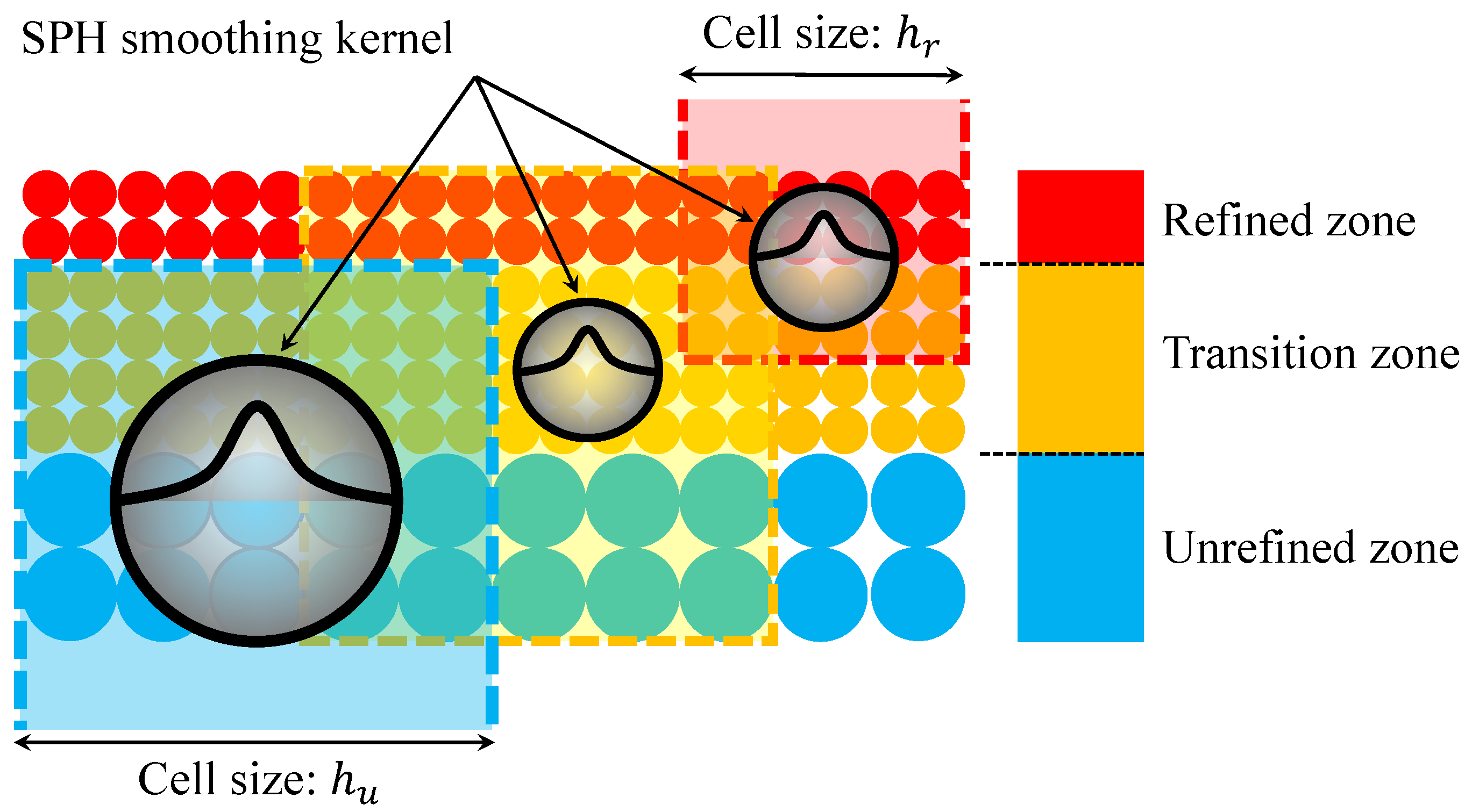
2.5. Dynamic Particle Refinement

The novelty offered by this work lies in reducing the computational cost of the SPH LPBF simulations via spatial adaptivity. We propose a simple algorithm to refine SPH particles dynamically and increase the spatial resolution. This approach follows the procedure elaborated upon in the SPH metal cutting adoption of Afrasiabi et al. [33], which is easy to implement and well-suited to the LPBF simulation. In brief, the refinement procedure is carried out via particle splitting to decrease the discretization size (i.e., increase the spatial resolution) in some regions of the computational domain. Here, a uniform mass splitting approach is used to conserve the mass and momentum of the system. More sophisticated mass splitting approaches can be found in [52,53].
Inspired by the multi-resolution SPH simulation of metal cutting in [33], the spatial adaptivity here occurs inside a moving frame in the vicinity of the laser processing area, where a cubic refinement pattern is chosen for particle splitting (see Figure 3). As far as an LPBF process is concerned, such a choice seems appropriate since the melt pool region is formed under the laser beam, and this is where the most challenging physics resides. The size of this frame can be sensitive to the configuration of the LPBF process, including the laser power, the beam radius, the powder bed geometry, and so on. Choosing proper dimensions for the refinement frame ensures that important areas (e.g., melting and re-solidification zones) are always discretized with the finest resolution available.
In this work, we proposed using an initial refinement frame with a width of 4 R centered at the laser focal point, where R is the laser beam radius. This frame moves at the same speed as the scanning laser. Only one stage of refinement is permitted here, meaning a refined particle will never be refined or coarsened again. Figure 3 displays a graphical abstract of the proposed particle refinement approach.
A second improvement of the present work stems from optimizing the nearest neighbor search algorithm within a multi-resolution domain. In particle-based simulations, using an efficient way to determine and organize neighbor particles is of vital importance. Previous multi-resolution SPH studies such as [33] rely on a cell-list structure where the size of each cell is twice the “maximum” smoothing length in the simulation. While this strategy is straightforward and ensures the completeness of particle interaction globally, the neighbor list of a particle would involve redundant particles in refined sub-domains. This paper, however, addresses this issue by reducing the cell size throughout the refined regions according to the “current” smoothing length instead of the “maximum” smoothing length. Therefore, a significant amount of unnecessary particle interactions in the refined sub-domains are avoided, and the computational performance of the code can be further enhanced. Figure 4 illustrates this optimization algorithm, where the choice of h r < h u provides a more efficient neighbor search.

3. Validation

The numerical results in this section are validated by comparing them to either an analytical solution or experimental data. For all cases, a quintic-spline kernel as in [36,54] is used. Please note that the code used for producing the present numerical results follows the main structure of the open-source SPH codes referenced in the “Supplementary Materials” section of this article.

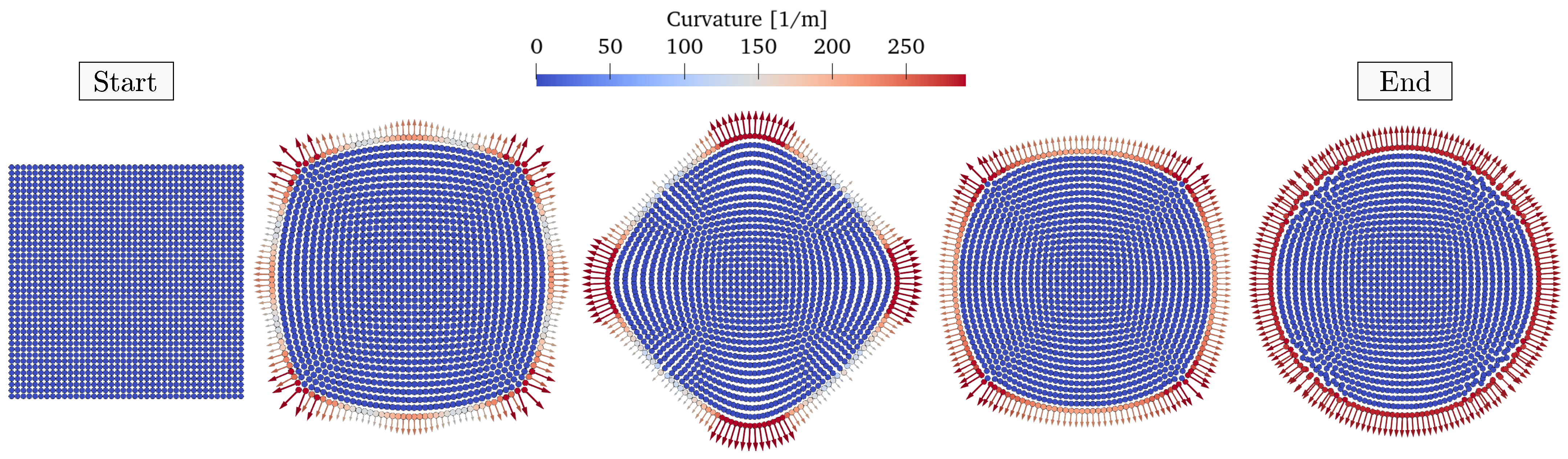
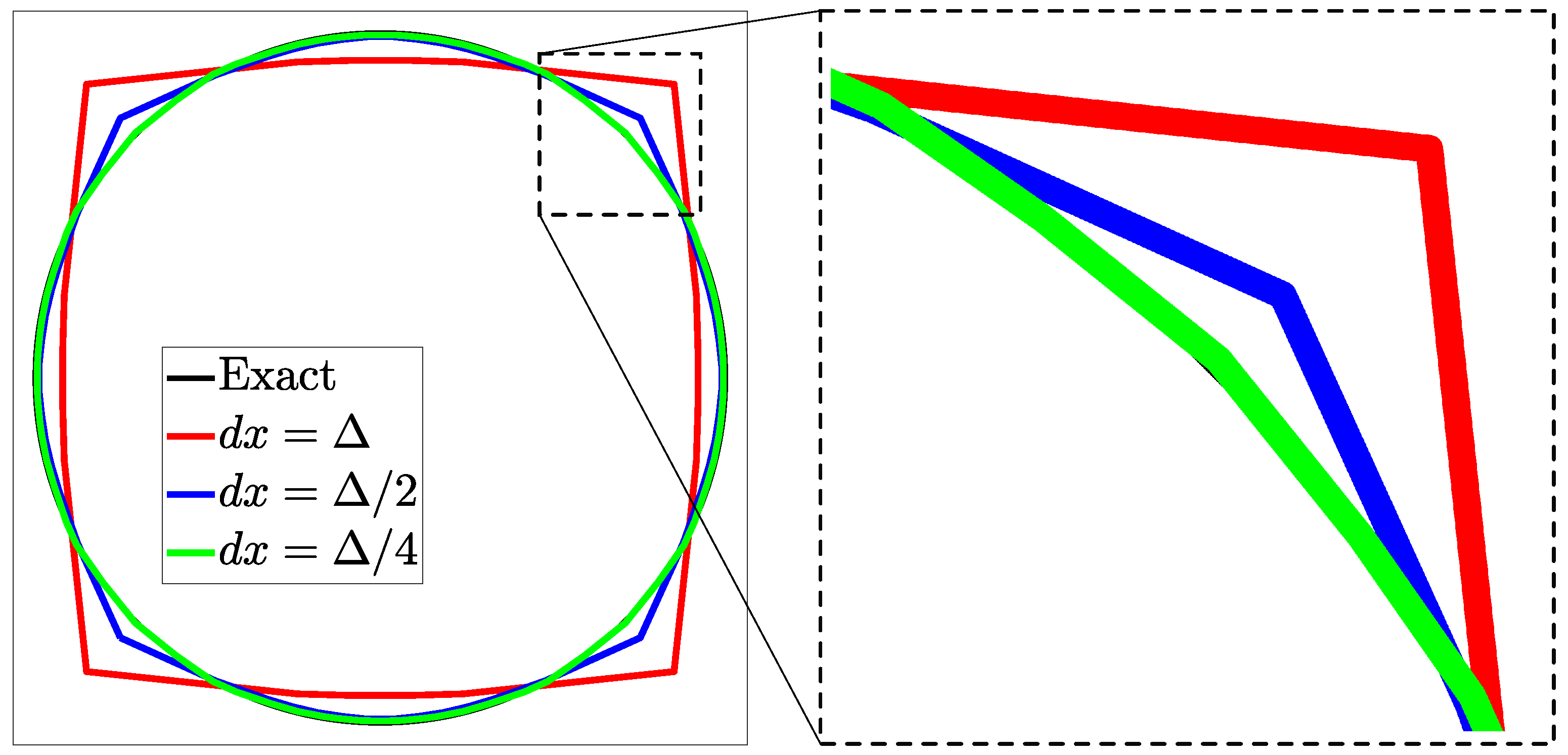
3.1. Liquid Droplet: Validation of Surface Tension

Surface tension plays a crucial role in LPBF processes. Therefore, it is necessary to investigate the method’s accuracy in approximating surface tension forces before applying it to a more complex problem. For this purpose, a surface-tension driven deformation of a liquid droplet in free space (i.e., no gravity) is examined. The initial geometry of the droplet is a square of size l = 1 cm. Properties of the liquid material are given in Table 1.
With the surface tension forces acting as a traction boundary condition, the initial square droplet reaches an equilibrium state by transforming into a circular shape. To capture this process within the SPH framework, the first term on the right-hand side of Equation (20) is exerted to one layer of free-surface particles in the normal direction. Figure 5 shows this evolution at 5 time steps using a total of 1600 uniform particles. For better visualization, the arrows are scaled to the magnitude of curvature at surface particles. At the last time step when t = 0.1 s, the SPH particles are at rest and turn into a nearly perfect circle, as expected.
The analytical solution is considered here by calculating the radius of the circular droplet at rest. Given the incompressible condition, this computation leads to a circle with R = 0.56 cm, which has the same area as the initial square geometry. To show the convergence of the method, the shape of this analytical circle is compared to the convex hull of the SPH particles at the last time step in 3 different resolutions. Figure 6 demonstrates this comparison, where Δ is the initial particle spacing for the lowest resolution case with a total of 100 SPH particles (i.e., Δ = 0.11 cm). The numerical result using d x = Δ / 4 and the exact solution in this figure are nearly identical and on top of each other, indicating the accuracy and convergence of the present method.

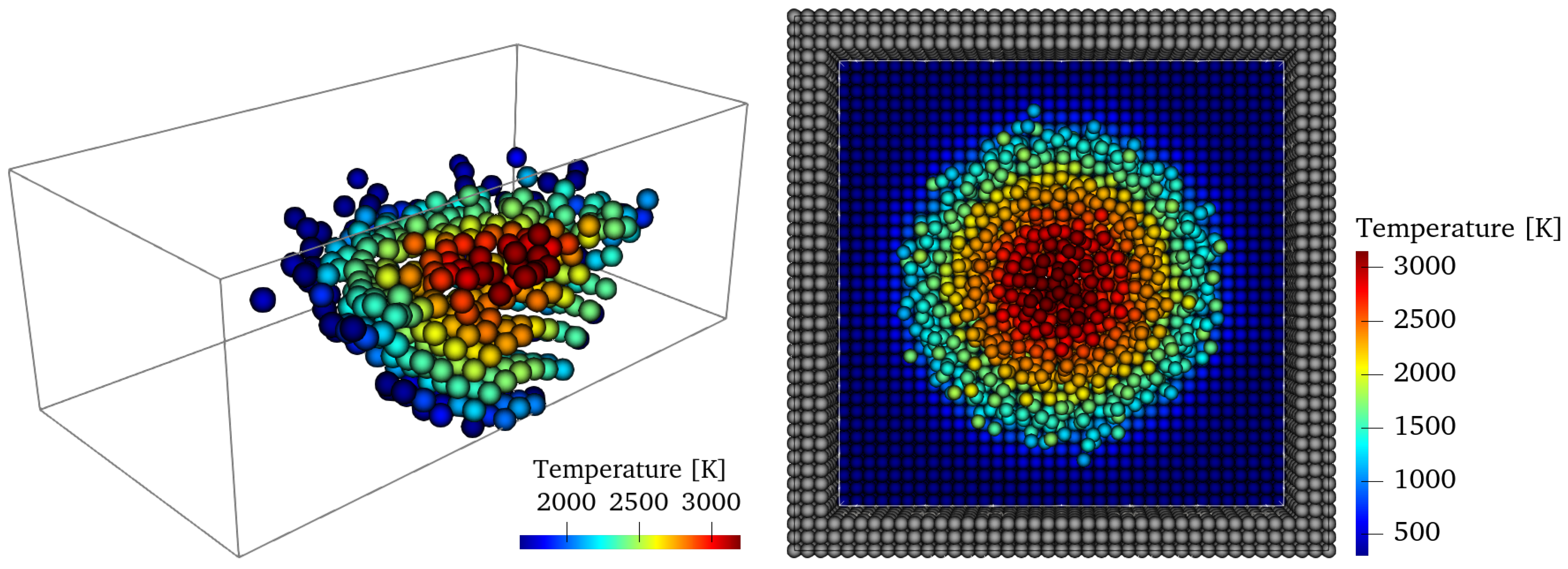
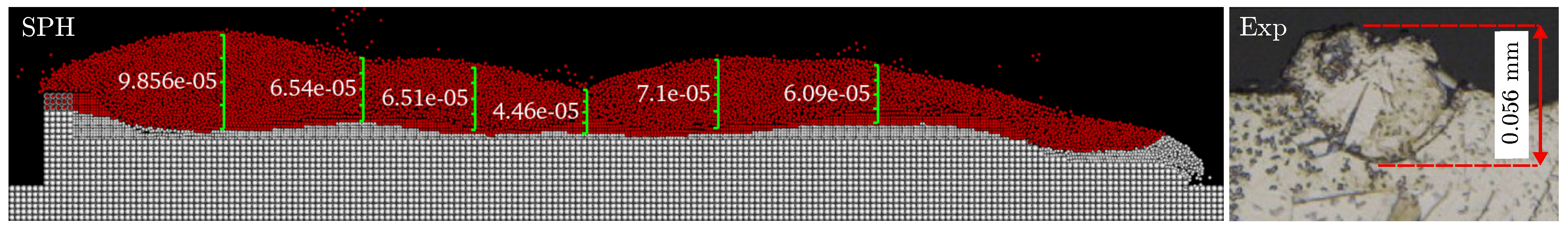
3.2. Weld Pool Experiment: Validation of Multiphysics Modeling

The laser spot welding experiments of He et al. [55] are taken as reference to validate the fully coupled thermal-mechanical-material model. Specifically, the test case pertains to a 304 stainless steel block welded by a laser pulse of power 1967 W, beam radius of 0.428 mm, and pulse duration of 3 ms. The workpiece is 1.3 mm by 1.3 mm and 0.4 mm height with material properties listed in Table 2. The convective heat transfer coefficient and emissivity factor are taken here as h c = 20 W/(m 2 · K) and ϵ = 0.4 , respectively. Expressed by Russell et al. [28], the reference density is considered herein to be a function of temperature:
ρ 0 ( T ) = 8020 0.50 ( T 298 ) solid 7332 6.03 ( T 1673 ) transition 6840 0.70 ( T 1773 ) liquid
To account for the thermo-capillary convection (i.e., Marangoni effect) at the melt-pool interface, the surface tension coefficient is also taken to be temperature-dependent. A common choice for σ ( T ) in this application was suggested by Sahoo et al. [56] as:
σ ( T ) = σ 0 A ( T T m ) R T Γ s log 1 + k l a s exp Δ H 0 R T
in which σ 0 = 1.943 N/m, A = 0.0005 N/(m · K), R = 8.3145 J/(mol · K), Γ s = 1.3 × 10 8  (kg · mol)/m 2 , k l = 0.0032 , and Δ H 0 = 166 × 10 3 J/(kg · mol). Together with the thermal gradient, this temperature-dependent coefficient is plugged in Equation (20) to approximate the tangential Marangoni surface tension force.
A 3D SPH model of this benchmark is created by discretizing the block with approximately 25k particles. This setup leads to a discretization size of d x = 0.045 mm and a time step in the order of 10 7 s. As for the thermal boundary conditions, a constant temperature of T 0 = 293 K is imposed on the bottom of the substrate (i.e., Dirichlet boundary condition). Furthermore, heat loss is included via radiation and convection to air through all open surfaces (i.e., Neumann boundary condition).
Figure 7 and Table 3 provide the simulation results of the weld pool geometry at t = 3 ms. We measured the radius and depth of the weld pool by a line distance calculator in ParaView. According to the data in Figure 7, the predicted weld pool dimensions are compared against the results from two other references, both experimental and computational, in Table 3. The comparison shows that the present values of weld pool dimension agree well with those of He et al. [55] and Russell et al. [28]. Also, the geometry of the weld pool simulated by SPH is similar to that of the physical experiment, clearly seen through the side-by-side comparison in Figure 7. Even at this fairly low resolution, the 3D SPH model predicts the depth of the weld pool by an error of 4% and its radius by 10%.
Another check on the model is performed by reporting the maximum temperature in the last time step. Figure 8 presents two snapshots for this purpose, showing the temperature distribution of the solidified SPH particles alongside a top view of the weld pool. It is observed that the maximum temperature in this simulation is 3152 K found at the center of the weld spot. This value is close to T m a x = 3200 K from the high-resolution SPH simulation of Dao and Lou [57] and the experimental measurement of He et al. [55].

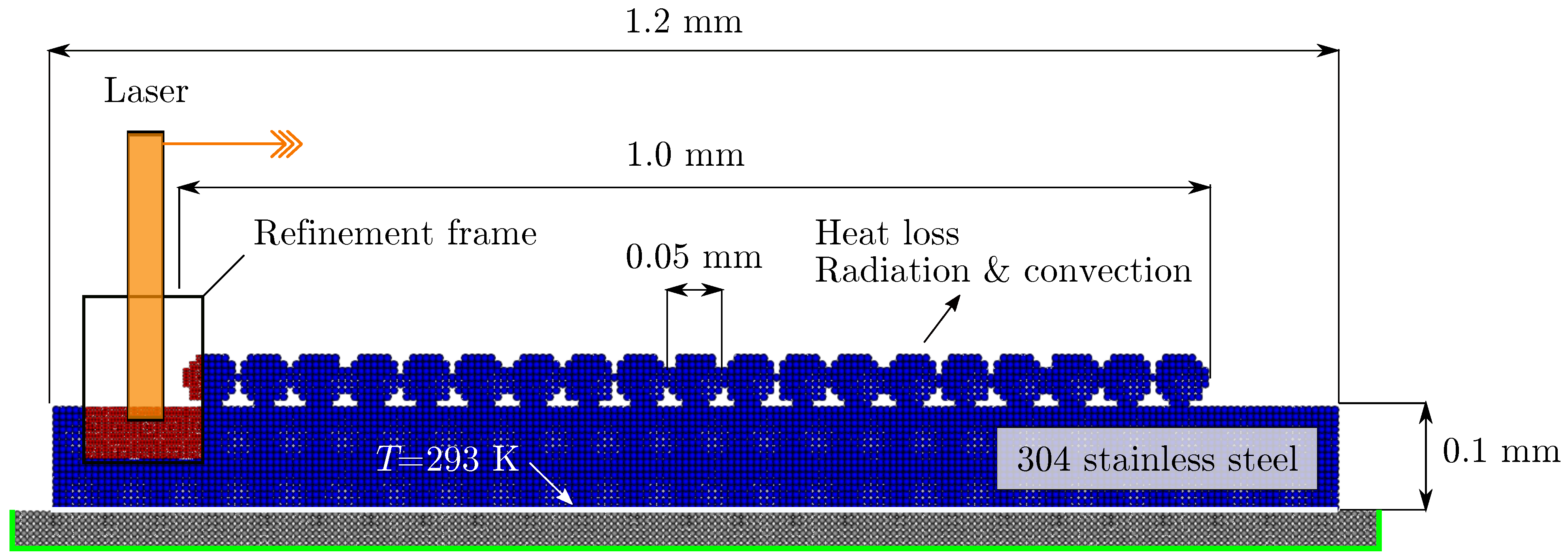
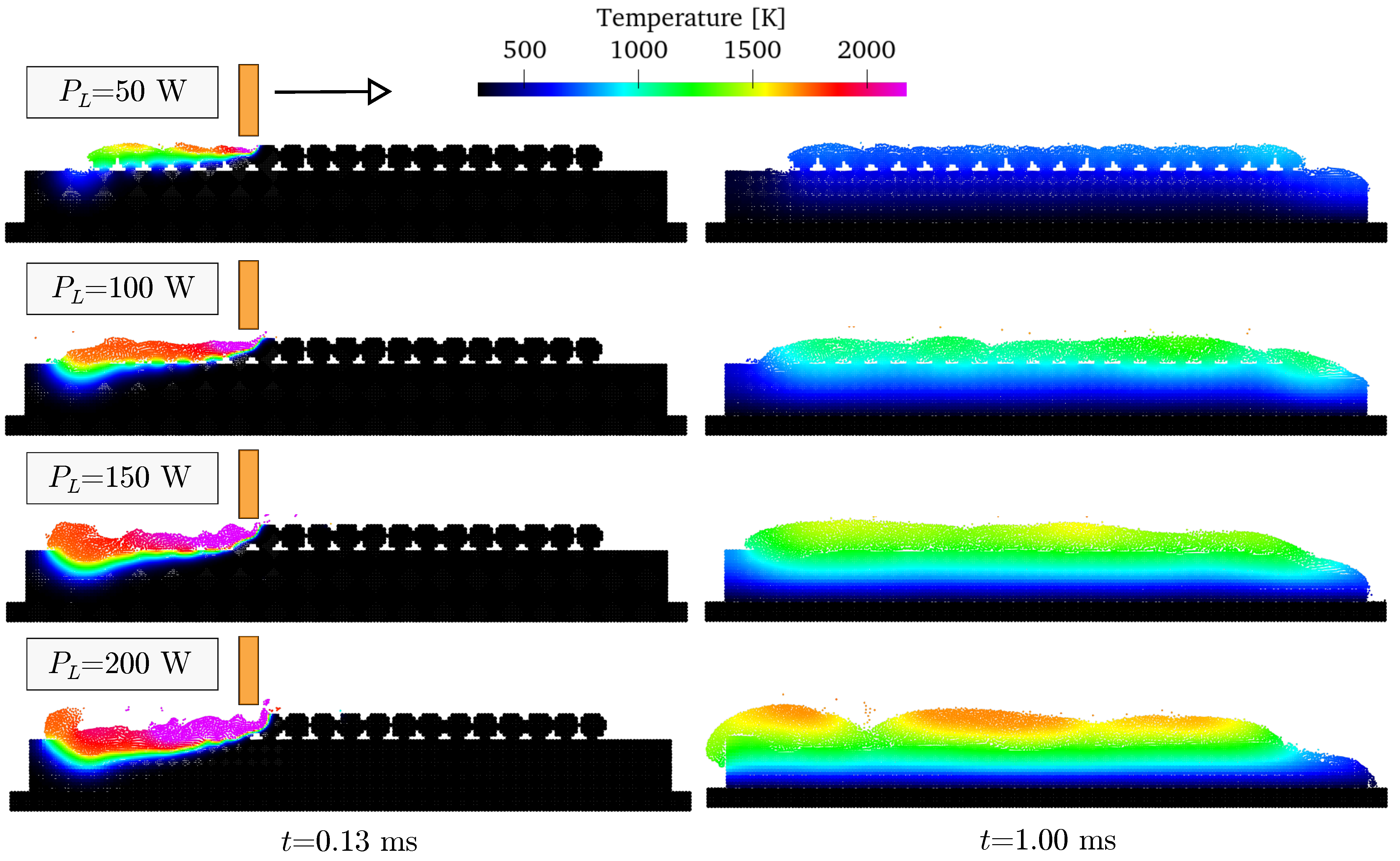
4. Application: Laser Powder Bed Fusion

The proposed multi-resolution SPH code is applied to simulate a 2D laser powder bed fusion (LPBF) process. Similar to the experimental setup of Khairallah and Anderson [12], the initial configuration is composed of a 304 stainless steel particle bed sitting on a flat substrate of the same material, with properties given in Equations (25) and (26) and Table 2. For the SPH simulation setup, one layer of circular powder particles with a diameter of 50  μ m is uniformly distributed on a 1 mm long track. Figure 9 shows the dimensions and boundary conditions of this problem. We terminate the simulation at around t = 1.13 ms to ensure that the powder bed is scanned and fully solidified.

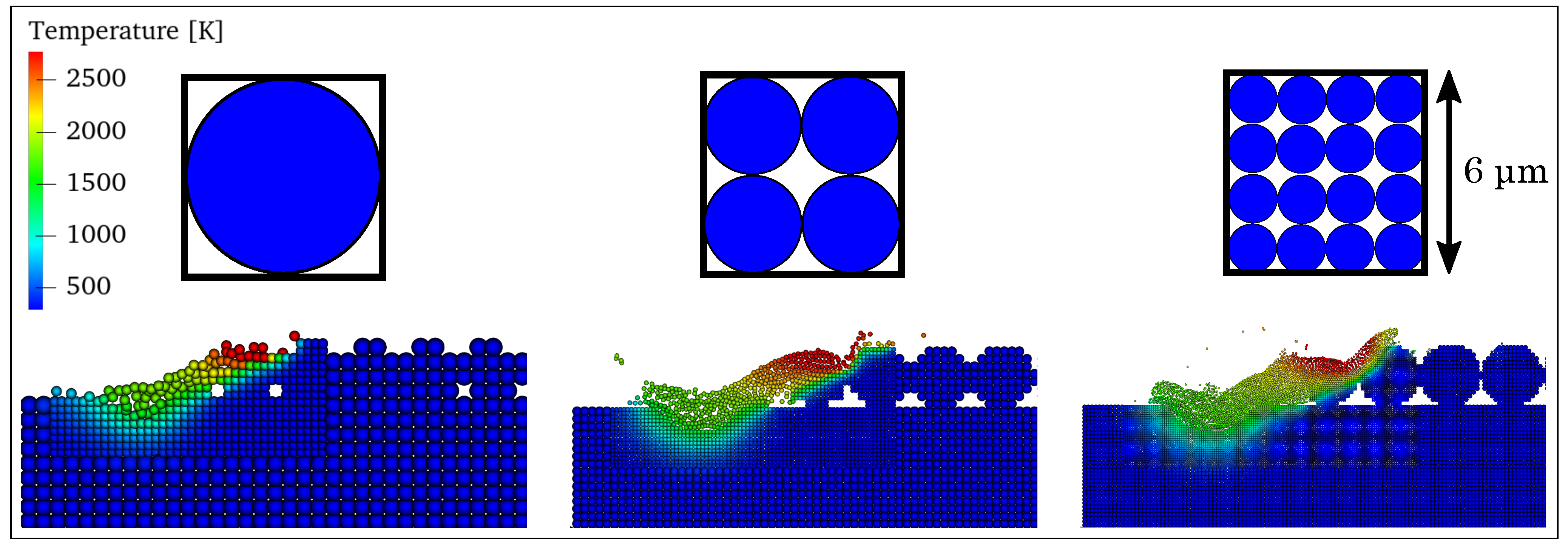
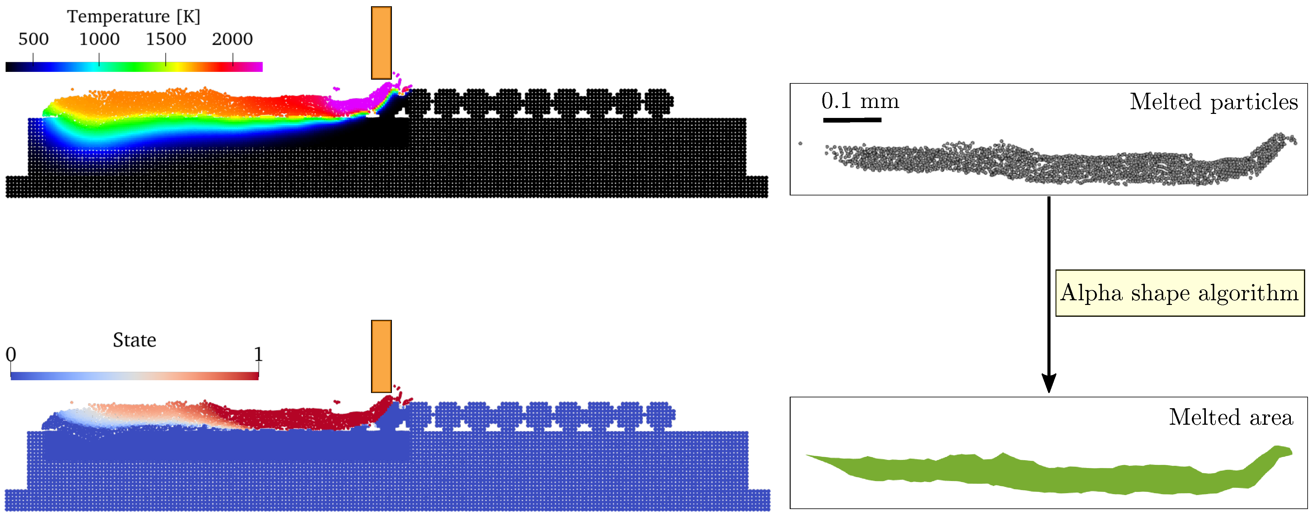
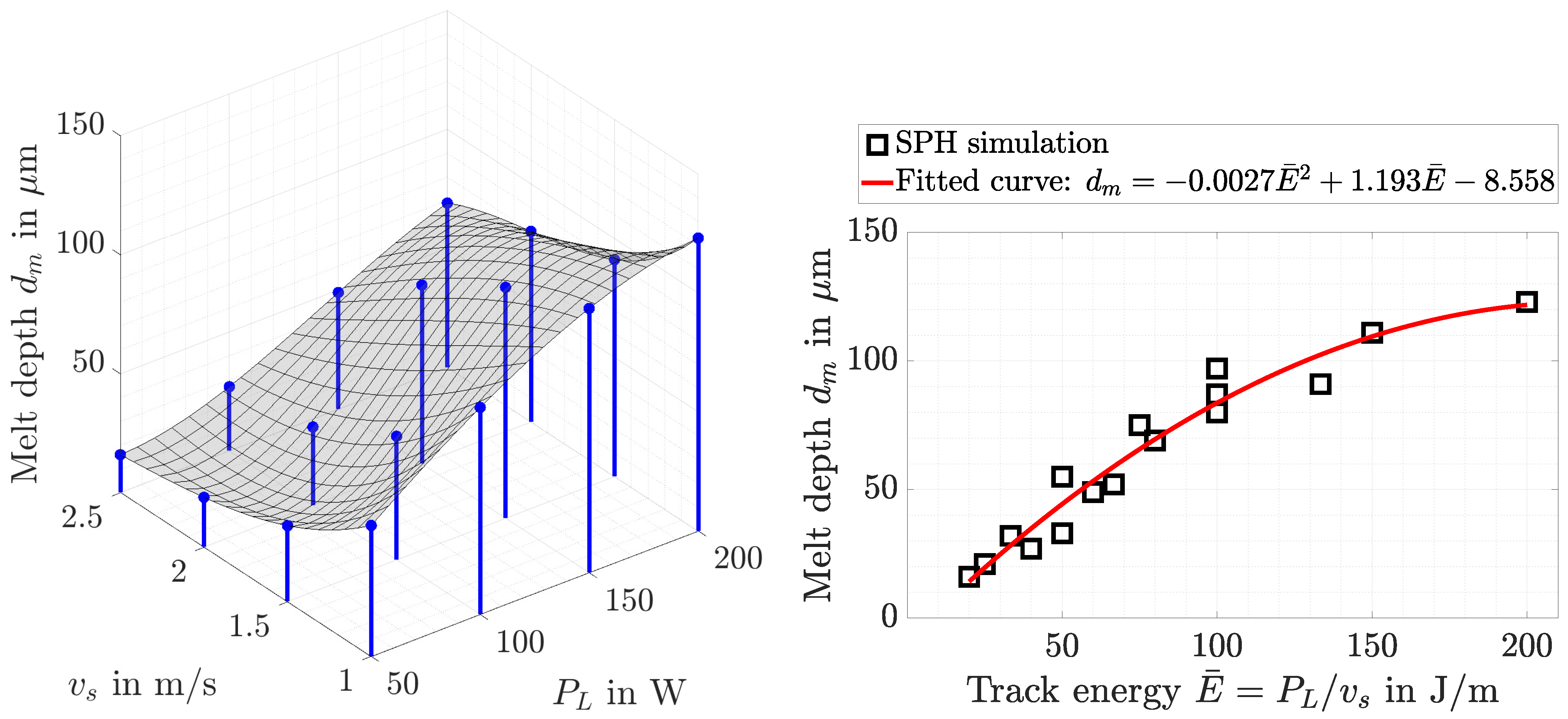
4.1. Parameter Study and Some General Observations

The presented spatial adaptivity algorithm helps achieve a more realistic LPBF simulation with less computational effort (see Figure 10). However, another incentive to introduce particle refinement into the current SPH LPBF models was to minimize their computational cost and allow for parameter studies in a reasonable amount of time. For instance, analyzing the sensitivity of melt pool dimensions to process parameters is a useful consideration that will assist in optimizing fabricated part quality. Therefore, the effect of the track energy on the melt geometry using the efficient SPH code is investigated in this section. According to the term used in [58], the track energy is defined here as E ¯ = P L / v s with respect to the laser power and scan speed.
Since SPH particles are incapable of representing the interface explicitly [54], a post-processing analysis needs to be performed to accurately extract the melt geometry. The α -shape algorithm of Edelsbrunner et al. [59] was chosen for this purpose. Figure 11 illustrates the calculation steps of the melt geometry as an α -shape, depicted in green. The procedure is showcased for a laser power of 100 W scanning the LPBF track at the speed of 1 m/s. Snapshots of the temperature and material phase are shown, where the state color-bar indicates the parameter s defined in Equation (22). The state scale is linear, starting from the liquid state represented by red, down to the solid state shown in blue. The SPH particles with temperatures equal or greater than the melt temperature are extracted, shown in solid grey on the right top frame. The α -shape algorithm is then applied to these melted particles to find an explicit definition of the melt pool interface.
Halfway through the scanning process, the melt pool seems to reach a steady state. SPH frames are thus taken from this time instant: after the laser has scanned half of the powder bed. It is clear from the state of SPH particles in Figure 11 that the laser beam (in orange) creates a highly dynamic melt pool underneath itself, fusing the powder bed along the way. A very similar behavior and zonal distinction were also observed by previous studies in FEM [12] and (single-resolution) SPH [28].
In order to set up the parameter study, a total of 16 test cases was simulated by varying the laser power from 50 to 200 W at different scan speeds of 1, 1.5, 2, and 2.5 m/s. The finest and coarsest discretization sizes in these models were, respectively, 3 μ m and 6 μ m. In Figure 12, the total melt depth d m is plotted in grey as a surface function of the laser power and scan speed. The blue stems in this plot indicate the 16 simulation data points. As expected, the maximum depth is found when using the maximum power (200 W) at the minimum scan speed (1 m/s). Moreover, a second-degree polynomial equation of d m expresses the best fit to the available track energies. The red curve in Figure 12 represents this graph alongside the SPH data-sets shown in black squares.
For a laser power of 200 W at the scan speed of 2 m/s, Figure 13 shows the melt dimensions after the powder bed is scanned and fully solidified. As a verification that the present SPH results are correct, the simulated LPBF track is plotted next to the experimental monograph of [12] for a very similar case. The numerical calculations are represented at six locations sufficiently far from the two edges to average the melt shape. We found the mean approximation error in the range of 15–20%. The diameter of fine SPH particles is ≈3 μ m and almost all melted sub-domains are discretized by this resolution (i.e., the red particles in Figure 13). In contrast to the LPBF simulation of Russell et al. [28], SPH particles ejected from the melt pool were not removed from the present model. A closer look at the red particles flying above the solidified track confirms this, clearly seen in Figure 13.
To generate deeper insight into the LPBF process, another sensitivity analysis on the laser power effects was carried out. For this purpose, powers varying from 50 to 200 W at a constant speed of 2.5 m/s were considered. A full representation is depicted in Figure 14 at t = 0.13 and t = 1 ms. Following from top to bottom, it becomes evident that increasing the power causes material sputtering and leads to worse surface roughness. The existence of voids between unmelted powders at P L = 50 W implies that this power is insufficient for fully melting the powder bed and penetrating into the substrate. On the other hand, the melt surface profile is significantly more volatile in the case of P L = 200 and necking can be observed at the solidified track. Overall, among these numerical experiments, scanning a 150-W laser at the speed of v s = 2.5 m/s for this LPBF setup seems to produce the best result with fewer manufacturing defects.

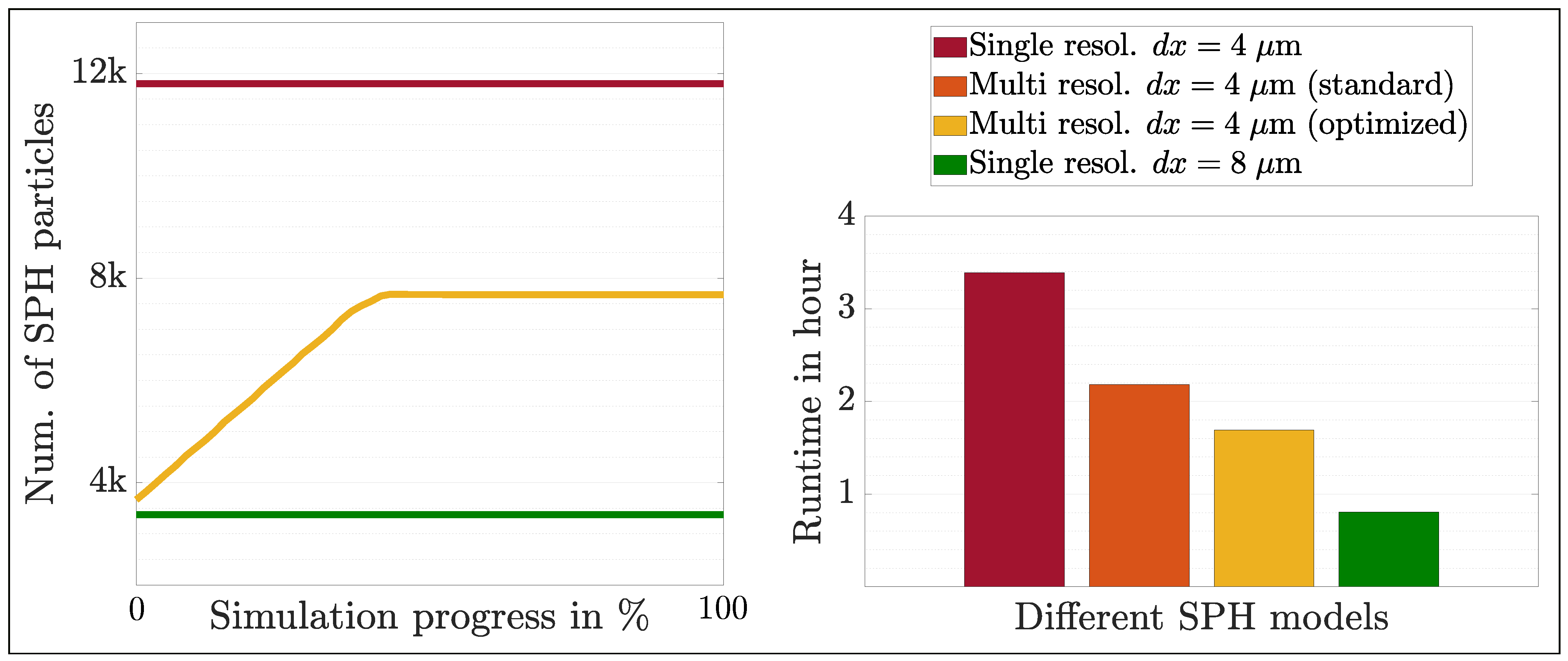
4.2. Computational Performance

To better appreciate the improvement gained by the proposed particle refinement approach, a runtime analysis was performed on 4 models:
  • Single resolution w/o dynamics particle refinement w/uniform discretization size  Δ / 2
  • Multi resolution w/dynamics particle refinement w/o neighbor-list optimization
  • Multi resolution w/dynamics particle refinement w/neighbor-list optimization
  • Single resolution w/o dynamics particle refinement w/uniform discretization size Δ
The simulation setup in all cases is the same as the reference model taken from [28], corresponding to a laser power of 100 W at the scan speed of 2 m/s using a discretization size of 4 μ m. Elapsed simulation times are recorded for a serial C++14 implementation, run on a single CPU core of Intel® Core™ i5–4690 at 3.50 GHz. Shown in Figure 15 is a comparison of the runtime associated with each model. The only difference between models 2 and 3 is using the optimized algorithm proposed for constructing the neighbor list of multi-resolution SPH particles (see in Section 2.5). This explains why the number of particles in both cases is the same (yellow graph of the left plot in Figure 15), but their runtime is different (orange vs. yellow graphs on the right plot in Figure 15). As can be seen, using the proposed optimization saves an additional 25% of the computational cost in multi-resolution SPH schemes. Consequently, a 2D LPBF simulation of a 1-mm long track with a reasonable discretization size of 4 μ m can be finished in almost 90 min.
On the other hand, both multi-resolution cases (models 2 and 3) could cut the final number of particles down to almost half of the reference case (model 1). The bar-chart comparison shows that the optimized multi-resolution simulation saves 50% of the computational time, thus 2× faster in providing the same result. Although not quite similar in terms of the computing platform and hardware, it is still beneficial to point out that the (single-resolution) SPH model of [28] published in 2018 was claimed to take 36 h on a single CPU core.

5. Conclusions

This paper developed an efficient multi-resolution SPH framework for numerical simulation of the LPBF process. Analytical and experimental validations were carried out to ensure the correct working of the code in a liquid droplet and laser spot welding test. The numerical results demonstrate the capability of the presented method in simulating the melt pool dynamics and capturing the relevant physics in an LPBF process. By enabling dynamic particle refinement within the SPH simulation, the proposed approach reduced the calculation time remarkably and facilitated further explorations such as parameter study and fine discretization. The results from this improvement are promising: Showcased for a 2D single-track LPBF case, almost 35% of the computational cost of SPH was saved without using the optimized neighbor-list algorithm. Using an optimized neighbor-search scheme resulted in a 15% additional saving and led to a 2× faster code with the same result. In brief, a 2D LPBF simulation of a 1-mm long track using SPH particles of 4 μ m diameter can now be completed in 90 min.
The use of SPH for AM simulation is a young but rapidly growing area of research, which opens up multiple new avenues for future developments. It is of utmost importance to strengthen the numerical model validation against physical experiments where more measurement data are available. The proposed scheme was presented for a 2D LPBF simulation but can be easily extended to 3D applications. Furthermore, the achieved saving in runtime is convincing to incorporate the dynamic refinement algorithm into the parallel SPH codes running on both CPUs and GPUs.

Supplementary Materials

The following are available at https://www.mdpi.com/article/10.3390/app11072962/s1. The software used for producing the results in this paper follows the implementation given in the following public source codes: “MFree IWF Cut Refine” (link: https://github.com/iwf-inspire/mfree_iwf-ul-cut-refine (accessed on 24 March 2021)) and “MFree IWF Thermal” (link: https://github.com/iwf-inspire/thermal_iwf (accessed on 24 March 2021)).

Author Contributions

M.A.: conceptualization, methodology, software, validation, formal analysis, investigation, data curation, visualization, writing, original draft preparation, and writing, review and editing. C.L.: software, data curation. M.B.: supervision, revision, project administration. K.W.: supervision, revision, project administration, and funding acquisition. All authors read and agreed to the published version of the manuscript.

Funding

The authors received no specific funding for this work.

Institutional Review Board Statement

Not applicable.

Informed Consent Statement

Not applicable.

Acknowledgments

The authors thank Matthias Röthlin, Hagen Klippel, and Eleni Chatzi for their support and invaluable discussions during this research project.

Conflicts of Interest

The authors declare no conflict of interest. The funders had no role in the design of the study; in the collection, analyses, or interpretation of data; in the writing of the manuscript; nor in the decision to publish the results.

Abbreviations

AMadditive manufacturing
CFDcomputational fluid dynamics
CPUcentral processing unit
FEMfinite element method
FVMfinite volume method
GPUgraphics processing unit
LBMLattice Boltzmann method
LPBFlaser powder bed fusion
PBFpowder bed fusion
SPHsmoothed particle hydrodynamics

References

  1. Gu, D.D.; Meiners, W.; Wissenbach, K.; Poprawe, R. Laser additive manufacturing of metallic components: Materials, processes and mechanisms. Int. Mater. Rev. 2012, 57, 133–164. [Google Scholar] [CrossRef]
  2. King, W.E.; Anderson, A.T.; Ferencz, R.M.; Hodge, N.E.; Kamath, C.; Khairallah, S.A.; Rubenchik, A.M. Laser powder bed fusion additive manufacturing of metals; physics, computational, and materials challenges. Appl. Phys. Rev. 2015, 2, 041304. [Google Scholar] [CrossRef]
  3. Lachmayer, R.; Lippert, R.B.; Fahlbusch, T. 3D-Druck beleuchtet. In Additive Manufacturing auf dem Weg in die Anwendung; Springer: Berlin/Heidelberg, Germany, 2016. [Google Scholar]
  4. Uriondo, A.; Esperon-Miguez, M.; Perinpanayagam, S. The present and future of additive manufacturing in the aerospace sector: A review of important aspects. Proc. Inst. Mech. Eng. Part G J. Aerosp. Eng. 2015, 229, 2132–2147. [Google Scholar] [CrossRef]
  5. Liu, R.; Wang, Z.; Sparks, T.; Liou, F.; Newkirk, J. Aerospace applications of laser additive manufacturing. In Laser Additive Manufacturing; Elsevier: Amsterdam, The Netherlands, 2017; pp. 351–371. [Google Scholar]
  6. Wohlers, T.T. Wohlers Report…: 3D Printing and Additive Manufacturing, State of the Industry, Annual Worldwide Progress Report; Wohlers Associates Incorporated: Auckland, New Zealand, 2014. [Google Scholar]
  7. Francis, M.P.; Kemper, N.; Maghdouri-White, Y.; Thayer, N. Additive manufacturing for biofabricated medical device applications. In Additive Manufacturing; Elsevier: Amsterdam, The Netherlands, 2018; pp. 311–344. [Google Scholar]
  8. Zaeh, M.F.; Branner, G. Investigations on residual stresses and deformations in selective laser melting. Prod. Eng. 2010, 4, 35–45. [Google Scholar] [CrossRef]
  9. Körner, C.; Attar, E.; Heinl, P. Mesoscopic simulation of selective beam melting processes. J. Mater. Process. Technol. 2011, 6, 978–987. [Google Scholar] [CrossRef]
  10. Khairallah, S.A.; Anderson, A.T.; Rubenchik, A.; King, W.E. Laser powder-bed fusion additive manufacturing: Physics of complex melt flow and formation mechanisms of pores, spatter, and denudation zones. Acta Mater. 2016, 108, 36–45. [Google Scholar] [CrossRef] [Green Version]
  11. Gürtler, F.-J.; Karg, M.; Leitz, K.-H.; Schmidt, M. Simulation of laser beam melting of steel powders using the three-dimensional volume of fluid method. Phys. Procedia 2013, 41, 881–886. [Google Scholar] [CrossRef] [Green Version]
  12. Khairallah, S.A.; Anderson, A. Mesoscopic simulation model of selective laser melting of stainless steel powder. J. Mater. Process. Technol. 2014, 214, 2627–2636. [Google Scholar] [CrossRef]
  13. Lee, Y.; Zhang, W. Mesoscopic Simulation of Heat Transfer and Fluid Flow in Laser Powder Bed Additive Manufacturing. In Proceedings of the 26th Solid Freeform Fabrication Symposium, Austin, TX, USA, 10–12 August 2015. [Google Scholar]
  14. Cook, P.S.; Murphy, A.B. Simulation of melt pool behaviour during additive manufacturing: Underlying physics and progress. Addit. Manuf. 2020, 31, 100909. [Google Scholar] [CrossRef]
  15. Lee, Y.; Zhang, W. Modeling of heat transfer, fluid flow and solidification microstructure of nickel-base superalloy fabricated by laser powder bed fusion. Addit. Manuf. 2016, 12, 178–188. [Google Scholar] [CrossRef] [Green Version]
  16. Dai, D.; Gu, D. Influence of thermodynamics within molten pool on migration and distribution state of reinforcement during selective laser melting of AlN/AlSi10Mg composites. Int. J. Mach. Tools Manuf. 2016, 100, 14–24. [Google Scholar] [CrossRef]
  17. Yuan, P.; Gu, D. Molten pool behaviour and its physical mechanism during selective laser melting of TiC/AlSi10Mg nanocomposites: Simulation and experiments. J. Phys. D Appl. Phys. 2015, 48, 035303. [Google Scholar] [CrossRef]
  18. Bidare, P.; Bitharas, I.; Ward, R.; Attallah, M.; Moore, A.J. Fluid and particle dynamics in laser powder bed fusion. Acta Mater. 2018, 142, 107–120. [Google Scholar] [CrossRef]
  19. Lucy, L.B. A numerical approach to the testing of the fission hypothesis. Astron. J. 1977, 82, 1013–1024. [Google Scholar] [CrossRef]
  20. Gingold, R.A.; Monaghan, J.J. Smoothed particle hydrodynamics: Theory and application to non-spherical stars. Mon. Not. R. Astron. Soc. 1977, 181, 375–389. [Google Scholar] [CrossRef]
  21. Röthlin, M.; Klippel, H.; Afrasiabi, M.; Wegener, K. Metal cutting simulations using smoothed particle hydrodynamics on the GPU. Int. J. Adv. Manuf. Technol. 2019, 102, 3445–3457. [Google Scholar] [CrossRef]
  22. Afrasiabi, M.; Meier, L.; Röthlin, M.; Klippel, H.; Wegener, K. GPU-accelerated meshfree simulations for parameter identification of a friction model in metal machining. Int. J. Mech. Sci. 2020, 176, 105571. [Google Scholar] [CrossRef]
  23. Roethlin, M.; Klippel, H.; Afrasiabi, M.; Wegener, K. Meshless single grain cutting simulations on the GPU. Int. J. Mechatronics Manuf. Syst. 2019, 12, 272–297. [Google Scholar] [CrossRef]
  24. Afrasiabi, M.; Klippel, H.; Roethlin, M.; Wegener, K. Smoothed Particle Hydrodynamics Simulation of Orthogonal Cutting with Enhanced Thermal Modeling. Appl. Sci. 2021, 11, 1020. [Google Scholar] [CrossRef]
  25. Afrasiabi, M.; Klippel, H.; Roethlin, M.; Wegener, K. Parameter Identification of a Friction Model in Metal Cutting Simulations with GPU-Accelerated Meshfree Methods. In Proceedings of the 14th World Congress on Computational Mechanics, Paris, France, 19–24 July 2020; pp. 1–12. [Google Scholar]
  26. Hu, H.; Eberhard, P. Thermomechanically coupled conduction mode laser welding simulations using smoothed particle hydrodynamics. Comput. Part. Mech. 2017, 4, 473–486. [Google Scholar] [CrossRef]
  27. Trautmann, M.; Hertel, M.; Füssel, U. Numerical simulation of TIG weld pool dynamics using smoothed particle hydrodynamics. Int. J. Heat Mass Transf. 2017, 115, 842–853. [Google Scholar] [CrossRef]
  28. Russell, M.; Souto-Iglesias, A.; Zohdi, T. Numerical simulation of Laser Fusion Additive Manufacturing processes using the SPH method. Comput. Methods Appl. Mech. Eng. 2018, 341, 163–187. [Google Scholar] [CrossRef]
  29. Park, C.Y.; Zohdi, T.I. Numerical modeling of thermo-mechanically induced stress in substrates for droplet-based additive manufacturing processes. J. Manuf. Sci. Eng. 2019, 141, 061001. [Google Scholar] [CrossRef]
  30. Afrasiabi, M.; Chatzi, E.; Wegener, K. A Particle Strength Exchange Method for Metal Removal in Laser Drilling. Procedia CIRP 2018, 72, 1548–1553. [Google Scholar] [CrossRef]
  31. Afrasiabi, M.; Wegener, K. 3D Thermal Simulation of a Laser Drilling Process with Meshfree Methods. J. Manuf. Mater. Process. 2020, 4, 58. [Google Scholar] [CrossRef]
  32. Fürstenau, J.P.; Wessels, H.; Weißenfels, C.; Wriggers, P. Generating virtual process maps of SLM using powder-scale SPH simulations. Comput. Part. Mech. 2020, 7, 655–677. [Google Scholar] [CrossRef]
  33. Afrasiabi, M.; Röthlin, M.; Klippel, H.; Wegener, K. Meshfree simulation of metal cutting: An updated Lagrangian approach with dynamic refinement. Int. J. Mech. Sci. 2019, 160, 451–466. [Google Scholar] [CrossRef]
  34. Monaghan, J.J. Smoothed particle hydrodynamics. Annu. Rev. Astron. Astrophys. 1992, 30, 543–574. [Google Scholar] [CrossRef]
  35. Wendland, H. Piecewise polynomial, positive definite and compactly supported radial functions of minimal degree. Adv. Comput. Math. 1995, 4, 389–396. [Google Scholar] [CrossRef]
  36. Liu, M.; Liu, G. Smoothed particle hydrodynamics (SPH): An overview and recent developments. Arch. Comput. Methods Eng. 2010, 17, 25–76. [Google Scholar] [CrossRef] [Green Version]
  37. Hu, X.; Adams, N.A. A multi-phase SPH method for macroscopic and mesoscopic flows. J. Comput. Phys. 2006, 213, 844–861. [Google Scholar] [CrossRef]
  38. Marrone, S.; Colagrossi, A.; Di Mascio, A.; Le Touzé, D. Analysis of free-surface flows through energy considerations: Single-phase versus two-phase modeling. Phys. Rev. E 2016, 93, 053113. [Google Scholar] [CrossRef] [PubMed]
  39. Cleary, P.W.; Monaghan, J.J. Conduction modelling using smoothed particle hydrodynamics. J. Comput. Phys. 1999, 148, 227–264. [Google Scholar] [CrossRef]
  40. Afrasiabi, M.; Roethlin, M.; Wegener, K. Contemporary Meshfree Methods for Three Dimensional Heat Conduction Problems. Arch. Comput. Methods Eng. 2020, 27, 1413–1447. [Google Scholar] [CrossRef]
  41. Gusarov, A.; Yadroitsev, I.; Bertrand, P.; Smurov, I. Model of radiation and heat transfer in laser-powder interaction zone at selective laser melting. J. Heat Transf. 2009, 131, 072101. [Google Scholar] [CrossRef]
  42. Antuono, M.; Colagrossi, A.; Marrone, S.; Molteni, D. Free-surface flows solved by means of SPH schemes with numerical diffusive terms. Comput. Phys. Commun. 2010, 181, 532–549. [Google Scholar] [CrossRef]
  43. Colagrossi, A.; Antuono, M.; Le Touzé, D. Theoretical considerations on the free-surface role in the smoothed-particle-hydrodynamics model. Phys. Rev. E 2009, 79, 056701. [Google Scholar] [CrossRef]
  44. Becker, M.; Teschner, M. Weakly compressible SPH for free surface flows. In Proceedings of the 2007 ACM SIGGRAPH/Eurographics Symposium on Computer Animation, San Diego, CA, USA, 2–4 August 2007; pp. 209–217. [Google Scholar]
  45. Afrasiabi, M.; Mohammadi, S. Analysis of bubble pulsations of underwater explosions by the smoothed particle hydrodynamics method. In Proceedings of the ECCOMAS International Conference on Particle Based Methods, Spain, Barcelona, 25–27 November 2009. [Google Scholar]
  46. Afrasiabi, M.; Roethlin, M.; Wegener, K. Thermal simulation in multiphase incompressible flows using coupled meshfree and particle level set methods. Comput. Methods Appl. Mech. Eng. 2018, 336, 667–694. [Google Scholar] [CrossRef]
  47. Afrasiabi, M.; Roethlin, M.; Chatzi, E.; Wegener, K. A Robust Particle-Based Solver for Modeling Heat Transfer in Multiphase Flows. In Proceedings of the ECCM-ECFD, Glasgow, UK, 11–15 June 2018. [Google Scholar]
  48. Brackbill, J.U.; Kothe, D.B.; Zemach, C. A continuum method for modeling surface tension. J. Comput. Phys. 1992, 100, 335–354. [Google Scholar] [CrossRef]
  49. Adami, S.; Hu, X.; Adams, N. A new surface-tension formulation for multi-phase SPH using a reproducing divergence approximation. J. Comput. Phys. 2010, 229, 5011–5021. [Google Scholar] [CrossRef]
  50. Hashemi, H.; Sliepcevich, C. A numerical method for solving two-dimensional problems of heat conduction with change of phase. Chem. Eng. Prog. Symp. Ser. 1967, 63, 34–41. [Google Scholar]
  51. Monaghan, J.J. Smoothed particle hydrodynamics. Rep. Prog. Phys. 2005, 68, 1703. [Google Scholar] [CrossRef]
  52. Feldman, J.; Bonet, J. Dynamic refinement and boundary contact forces in SPH with applications in fluid flow problems. Int. J. Numer. Methods Eng. 2007, 72, 295–324. [Google Scholar] [CrossRef]
  53. Vacondio, R.; Rogers, B.; Stansby, P.; Mignosa, P. Variable resolution for SPH in three dimensions: Towards optimal splitting and coalescing for dynamic adaptivity. Comput. Methods Appl. Mech. Eng. 2016, 300, 442–460. [Google Scholar] [CrossRef]
  54. Afrasiabi, M. Thermomechanical Simulation of Manufacturing Processes Using GPU-Accelerated Particle Methods. Ph.D. Thesis, ETH Zurich, Zurich, Switzerland, 2020. [Google Scholar]
  55. He, X.; Fuerschbach, P.; DebRoy, T. Heat transfer and fluid flow during laser spot welding of 304 stainless steel. J. Phys. D Appl. Phys. 2003, 36, 1388. [Google Scholar] [CrossRef]
  56. Sahoo, P.; Debroy, T.; McNallan, M. Surface tension of binary metal—Surface active solute systems under conditions relevant to welding metallurgy. Metall. Trans. B 1988, 19, 483–491. [Google Scholar] [CrossRef]
  57. Dao, M.H.; Lou, J. Simulations of Laser Assisted Additive Manufacturing by Smoothed Particle Hydrodynamics. Comput. Methods Appl. Mech. Eng. 2021, 373, 113491. [Google Scholar] [CrossRef]
  58. Weirather, J.; Rozov, V.; Wille, M.; Schuler, P.; Seidel, C.; Adams, N.A.; Zaeh, M.F. A smoothed particle hydrodynamics model for laser beam melting of Ni-based alloy 718. Comput. Math. Appl. 2019, 78, 2377–2394. [Google Scholar] [CrossRef]
  59. Edelsbrunner, H.; Kirkpatrick, D.; Seidel, R. On the shape of a set of points in the plane. IEEE Trans. Inf. Theory 1983, 29, 551–559. [Google Scholar] [CrossRef] [Green Version]
Figure 1. Main physical processes in melt-pool region during powder bed fusion of LPBF.
Applsci 11 02962 g001
Figure 2. Illustration of the volumetric heat source modeling approach and the laser intensity distribution.
Applsci 11 02962 g002
Figure 3. Schematic illustration of the particle refinement approach: (Left) demonstrating the situation before and after splitting, where particle p meets the refinement criterion and is split into 4 smaller particles via a square splitting pattern; (Right) showing how the proposed refinement strategy works for an LPBF application. The initial refinement frame has a width of 4 R , where R is the laser beam radius. Particles with lower mass are depicted in blue and with smaller size.
Applsci 11 02962 g003
Figure 4. Graphical illustration of the proposed cell optimization for multi-resolution SPH domains.
Applsci 11 02962 g004
Figure 5. Deformation of a square droplet to a circle under the effect of surface tension.
Applsci 11 02962 g005
Figure 6. Convergence of the SPH results to the analytical solution in a liquid droplet test.
Applsci 11 02962 g006
Figure 7. Numerical and experimental weld pool Geometry for laser power of 1967 W, beam radius of 0.428 mm, and pulse duration of 3 ms including: (Left) weld pool cross sections in a side-by-side comparison of SPH result with experiment of He et al. [55]; (Right) top view of the whole domain showing the diameter of the laser weld spot.
Applsci 11 02962 g007
Figure 8. Temperature distribution at t = 3 ms for: (Left) SPH particles with temperatures higher than the melting temperature of the material; (Right) top view of the full domain including all particles.
Applsci 11 02962 g008
Figure 9. Initial configuration and boundary conditions of the LPBF simulation. A Gaussian laser beam is scanning the track from left to right, shown in orange. The size (i.e., mass) of each SPH particle inside the refinement frame is 1/4 of the unrefined particles in blue.
Applsci 11 02962 g009
Figure 10. Effect of spatial discretization on SPH results. Particle refinement leads to a more accurate melt surface in LPBF simulation. The blue particles inside the squares represent the finest resolution in each case.
Applsci 11 02962 g010
Figure 11. Melt pool formation and calculation of the melted area for the case of P L = 100 W and v s = 1 m/s after the laser has scanned half of the powder bed.
Applsci 11 02962 g011
Figure 12. Prediction of the melt depth using the proposed multi-resolution SPH approach.
Applsci 11 02962 g012
Figure 13. Melt dimensions for P L = 200 W at v s = 2 m/s when the track is fully solidified. The melted and re-solidified SPH particles are shown in red, obtained from the present multi-resolution SPH simulation at t = 1.25 ms. The numerical melt depth and height are represented at 6 locations (green line segments). The experimental micrograph reprinted from Khairallah and Anderson [12] Copyright (2021), with permission from Elsevier under License Number 5013001359377.
Applsci 11 02962 g013
Figure 14. Laser tracks with different powers at scan speed 2.5 m/s. Snapshots of the temperature distribution shown at t = 0.13 ms, when 1/3 of the powder-bed length is melted, and at t = 1.0 ms, when the LPBF track is fully solidified. The color-bar limit is set to a maximum of 2173 K for better visualization. The SPH particles are dynamically refined in all simulations, where the coarsest and finest discretization size used is 6 and 3 μ m, respectively.
Applsci 11 02962 g014
Figure 15. Runtime performance comparison. The proposed multi-resolution model (with optimized neighbor list) outperforms the other models by reducing approximately 50% of the computational cost of the reference model (i.e., single high resolution with d x = 4 μ m). The total number of SPH particles used by the multi-resolution model is 3668 at the beginning and 7658 at the end of the simulation, significantly lower than a total of 11,800 particle used by the reference model 1.
Applsci 11 02962 g015
Table 1. Properties of water used in the SPH simulation.
DensityDynamic ViscositySurface Tension Coefficient
Symbol ρ μ σ
Unitkg/m 3 Pa·sN/m
Value10000.0011
Table 2. Material properties used for the weld pool simulation, according to [28].
PropertySymbolUnitSolidLiquid
Dynamic viscosity μ Pa · s1.00.01
Heat conductivitykW/(m · K)20.93209.3
Specific heat capacity c p J/(kg · K)711.2937.4
Melting temperature T m K1732
Evaporation temperature T e K3100
Melting bandwidth δ T K100
Absorption coefficient a L 0.27
Table 3. Comparison of the weld pool dimensions: SPH vs. experiment.
DimensionPresent SPHRussell et al. SPH [28]Hu et al. Experiment [55]
Radius in mm (% error)0.43 (−10%)0.46 (−4%)0.48
Depth in mm (% error)0.27 (+4%)0.25 (−4%)0.26
Publisher’s Note: MDPI stays neutral with regard to jurisdictional claims in published maps and institutional affiliations.

