Performance of Envelope Demodulation for Bearing Damage Detection on CWRU Accelerometric Data: Kurtogram and Traditional Indicators vs. Targeted a Posteriori Band Indicators

Featured Application

Case Western Reserve University Bearing Data Center.

Abstract

Envelope demodulation of vibration signals is surely one of the most successful methods of analysis for highlighting diagnostic information of rolling element bearings incipient faults. From a mathematical perspective, the selection of a proper demodulation band can be regarded as an optimization problem involving a utility function to assess the demodulation performance in a particular band and a scheme to move within the search space of all the possible frequency bands {f, Δf} (center frequency and band size) towards the optimal one. In most of cases, kurtosis-based indices are used to select the proper demodulation band. Nevertheless, to overcome the lack of robustness to non-Gaussian noise, different utility functions can be found in the literature. One of these is the kurtosis of the unbiased autocorrelation of the squared envelope of the filtered signal found in the autogram. These heuristics are usually sufficient to highlight the defect spectral lines in the demodulated signal spectrum (i.e., usually the squared envelope spectrum (SES)), enabling bearings diagnostics. Nevertheless, it is not always the case. In this work, then, posteriori band indicators based on SES defect spectral lines are proposed to assess the general envelope demodulation performance and the goodness of traditional indicators. The Case Western Reserve University bearing dataset is used as a test case.

1. Introduction

Rolling element bearings (REBs) are fundamental components of most power transmission systems involving rotating shafts, and as such, it is also important that they are monitored so as to avoid catastrophic accidents. An effective way that emerged, among the others, for the diagnostics of REBs is vibration monitoring [1].

In fact, vibration signals exhibit damage-characteristic signatures: in the time domain, series of transients (i.e., impulse responses) could be found to repeat at specific defect frequencies that depended on the defect location (i.e., the rolling element, the outer or inner rings or the cage) [2]. Unfortunately, such sharp and short duration transients are usually covered by background noise or by other common contributions to the overall machine vibration signature (i.e., gears). Incipient damages signatures are usually so weak that they are not detectable even in the frequency domain spectra. Nevertheless, when the characteristic repetitive transients excite high-frequency resonances within the transmission path, an envelope demodulation performed in the resonance frequency band can enhance the signal-to-noise ratio of the bearing-characteristic signal. This technique is known as the high-frequency resonance technique [3] or envelope demodulation.

The selection of an appropriate demodulation band, usually called the informative frequency band (IFB), is then a fundamental issue for finding the best squared envelope spectrum (SES). From a mathematical perspective, the selection of such an IFB can be regarded as an optimization problem involving a utility function to assess the demodulation performance in a particular band and a scheme to move within the search space of all the possible frequency bands (f,Δf) (center frequency and band size) towards the optimal one.

Milestones for the band selection task are the spectral kurtosis (SK) [4] and the kurtogram [5], which uses as indicator (i.e., utility function) the kurtosis of the coefficients at the output of quasi-analytic filters with different central frequencies CF and bandwidths BF. This idea led to the fast kurtogram (FK) algorithm [6], based on the computation of the utility function over a discrete paving of the (f,Δf) plane built with a multirate filter bank. The consequent fixed discrete partitioning is computationally very efficient, but could sometimes be limiting. Hence, a more flexible band selection was proposed in [7] using a genetic algorithm to directly optimize the Finite Impulse Response (FIR) filter parameters against a kurtosis-based utility function. To enhance band separation on the contrary, wavelet packet transform (WPT) was proposed in [8].

The main limit of the kurtosis, in any event, was recognized to be its vulnerability to non-Gaussian noise and its tendency to decrease when the transient’s repetition rate increases [9]. Several different variations were then proposed. In [10], for example, a frequency-domain “protrusion” was introduced in the protrugram. In this case the utility function corresponds to the kurtosis of the amplitudes of the envelope spectrum of the demodulated signal. Likewise, the kurtosis of the power spectrum of the envelope of the wavelet packet transform (WPT) filtered signal was proposed in [11]. Nevertheless, the protrugram, as the kurtogram, is the maximum for a single harmonic in the SES, so it is still not ideal for the detection of repetitive transients.

The sparsogram defined in [12] proposes, on the contrary, a measure of spectral sparsity (i.e., the ratio of L2 and L1 norm of the squared envelope spectrum (SES)) was used to define the sparsogram. An in-depth study of spectral L2/L1 norm can be found in [13] to explain the closeness of SK with spectral squared L2/L1 norm and with spectral correlation (SC) [14], a key approach of cyclic spectral analysis (CSA) [15] together with the cyclic modulation spectrum (CMS) [16], later generalized into the Fast-SC [17], a fast estimator of SC.

Other indices, derived from different fields, can be found in the literature to improve the kurtogram. The Gini index, for example, originally meant to produce a measure of wealth inequality (i.e., sparseness, similarly to the idea of spectral L2/L1 norm [18]), was derived from econometrics by [19] to improve the resistance to noisy random impulses.

Derived from physics, a characterization of both time- and frequency-domain impulsiveness can be found in the infogram [20], based on the negentropy of the Squared Envelope and on the negentropy of the Squared Envelope Spectrum, averaged to characterize both the impulsive and cyclostationary signatures of the repetitive transients.

A modification of the traditional kurtosis was proposed in [21], where the correlated kurtosis (CK) was proved to improve the sensitivity to the repetitive impulses typical of the bearing signature [22]. This technique is not completely blind, but requires the use of the periodicity of the impulses as an input.

Other targeted methods which require assumptions about the periodicity of fault symptoms and exploit the relationship between cyclostationarity and envelope analysis are the envelope-based cyclic periodogram [23] and the log-cycligram [24], which was proved to be robust to highly impulsive noise [25].

A method which is blind but takes advantage of the cyclostationarity of the signal in a different way is the autogram. In [26], the kurtosis is not computed on the squared envelope itself, but on the unbiased autocorrelation of the squared envelope of the filtered signal. This allows it to overcome the lack of robustness to non-Gaussian noise of the traditional kurtogram. A computationally more efficient implementation is described in [27]. An analogous frequency domain approach is proposed in [28] where a modified protrugram is found from the computation of the kurtosis of the autocorrelation of the envelope spectrum.

Given the huge variety of algorithms presented in the literature survey, the present work sets two goals: to evaluate the general effectiveness of envelope demodulation and to assess the performance of common band-selection indicators against novel a posteriori indicators tailored for the purpose. The well-known Case Western Reserve University bearing dataset will be used as a test case.

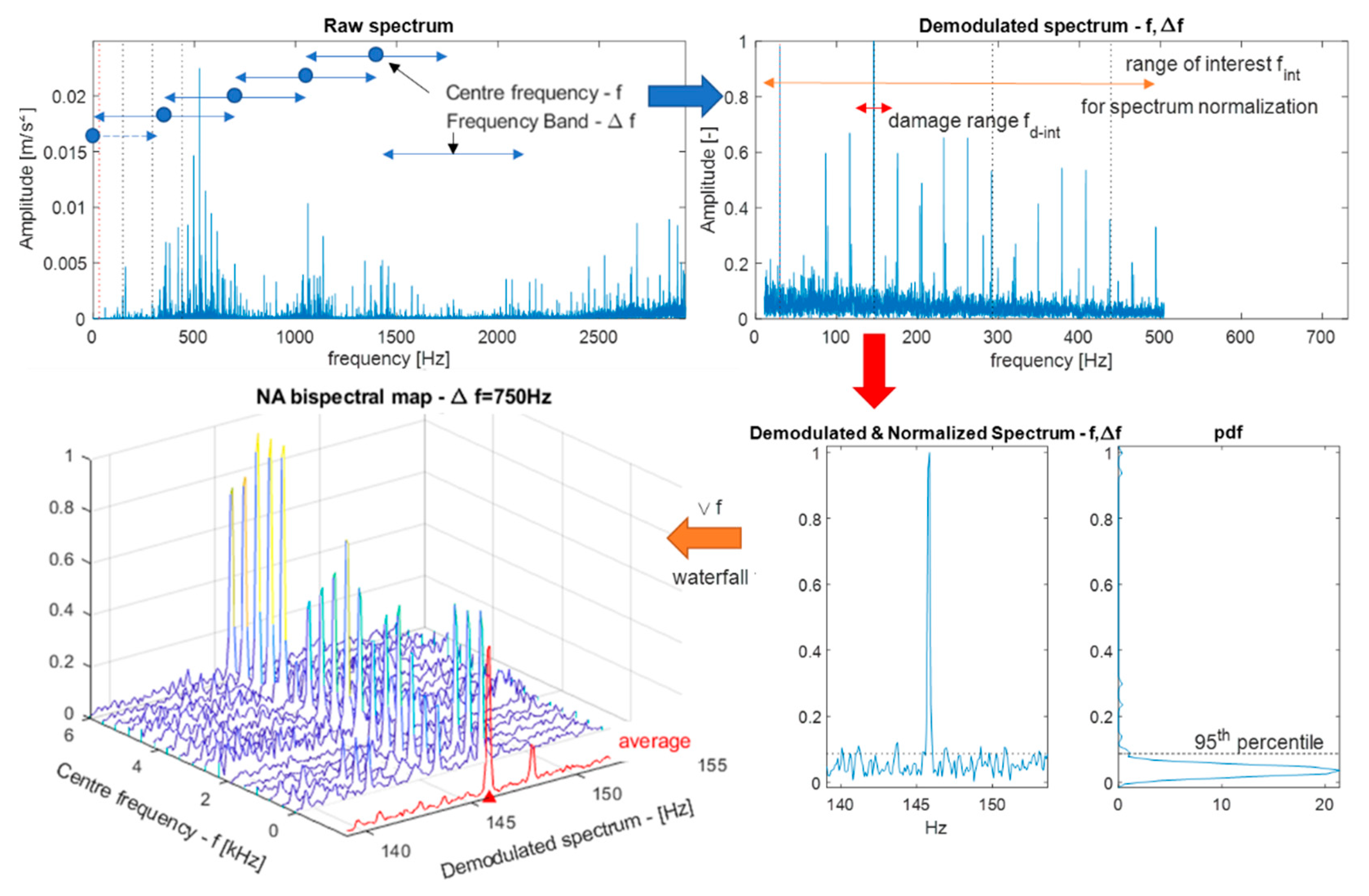
2. Methodology and Band Indicators

In this paper, the bearing diagnostics is regarded as an optimization problem based on the vibration signal x[n], assumed with a null mean value. The goal was to find the best combination of center frequency and band size (f,Δf) for filtering such a signal before envelope demodulation so that the damage-characteristic signature is maximized in the resulting SES.

According to the FK and most of the subsequent 2-D color maps found in the literature, the (f,Δf) plane is partitioned with a multirate filter bank, so that each part of the paving has a corresponding filtered signal x_{f,Δf}[n] whose envelope $E{x}_{\left\{\mathrm{f},\Delta \mathrm{f}\right\}}\left[n\right]=\left|x_{\left\{\mathrm{f},\Delta \mathrm{f}\right\}}\left[n\right]+i \mathscr{H}\left(x_{\left\{\mathrm{f},\Delta \mathrm{f}\right\}}\left[n\right]\right)\right|$ can be easily estimated. Note that i stands for the imaginary unit and $\mathscr{H}$ means Hilbert transform. In most of cases, the Squared Envelope $SE{x}_{\left\{\mathrm{f},\Delta \mathrm{f}\right\}}\left[n\right]={\left(E{x}_{\left\{{\mathrm{f}}^{*},{\Delta \mathrm{f}}^{*}\right\}}\left[n\right]\right)}^2$ is actually computed, as this can in principle reduce the demodulation aliasing due to the cusps in the $\left|\sin \vartheta \right|$ function (i.e., the Fourier basis) [29]. Nevertheless, the optimization is carried out by maximizing a band indicator (i.e., the kurtosis) over the entire paving so as to find the optimal {f,Δf} = {f*,Δf*}. Finally, the envelope demodulation is carried out by computing the spectrum of the signal filtered in the optimal {f*,Δf*} to obtain an envelope spectrum: $ES{x}_{\left\{{\mathrm{f}}^{*},{\Delta \mathrm{f}}^{*}\right\}}\left[\mathrm{k}\right]=\left|\mathrm{DFT}\left\{SE{x}_{\left\{{\mathrm{f}}^{*},{\Delta \mathrm{f}}^{*}\right\}}\left[n\right]\right\}\right|$ or a squared envelope spectrum: $SES{x}_{\left\{{\mathrm{f}}^{*},{\Delta \mathrm{f}}^{*}\right\}}\left[\mathrm{k}\right]={\left|\mathrm{DFT}\left\{SE{x}_{\left\{{\mathrm{f}}^{*},{\Delta \mathrm{f}}^{*}\right\}}\left[n\right]\right\}\right|}^2$, as in most of situations this improves the signal to noise ratio (SNR) [29].

According to the literature review in Section 1, the main blind band-selection indicators are reported:

• Spectral kurtosis (kurtogram [4,5,6]):

  $$\begin{gathered} K\left(f,\Delta f\right)=\frac{m_4\left\{E{x}_{\left\{\mathrm{f},\Delta \mathrm{f}\right\}}\left[n\right]\right\}}{{\left(m_2\left\{E{x}_{\left\{\mathrm{f},\Delta \mathrm{f}\right\}}\left[n\right]\right\}\right)}^2 } \\ {m}_r\left\{y\left[n\right]\right\}=\frac{1}{N}{{\displaystyle \sum }}_{n=1}^N{\left(y\left[n\right]\right)}^r \end{gathered}$$

  (1)

  where m_r{y[n]} represents the rth order moment of a generic discrete signal y[n].
• Protrusion (protrugram [10]):

  $$P\left(f,\Delta f\right)=\frac{m_4\left\{ES{x}_{\left\{\mathrm{f},\Delta \mathrm{f}\right\}}\left[n\right]\right\}}{{\left(m_2\left\{ES{x}_{\left\{\mathrm{f},\Delta \mathrm{f}\right\}}\left[n\right]\right\}\right)}^2 }$$

  (2)
• Spectral L2/L1 sparsity (sparsogram [12]):

  $$\begin{gathered} L_2/L_1\left(f,\Delta f\right)=\frac{L_2\left\{ES{x}_{\left\{\mathrm{f},\Delta \mathrm{f}\right\}}\left[\mathrm{k}\right]\right\}}{L_1\left\{ES{x}_{\left\{\mathrm{f},\Delta \mathrm{f}\right\}}\left[\mathrm{k}\right]\right\}}=\frac{\sqrt{{{\displaystyle \sum }}_{k=1}^{K=\frac{fs}{2}}{\left(ES{x}_{\left\{\mathrm{f},\Delta \mathrm{f}\right\}}\left[\mathrm{k}\right]\right)}^2}}{{{\displaystyle \sum }}_{k=1}^{K=\frac{fs}{2}}\left|ES{x}_{\left\{\mathrm{f},\Delta \mathrm{f}\right\}}\left[\mathrm{k}\right]\right|} \\ {L}_r\left\{y\left[n\right]\right\}={\left({{\displaystyle \sum }}_{n=1}^N{\left(\left|y\left[n\right]\right|\right)}^r\right)}^{1/r} \end{gathered}$$

  (3)

  where L_r{y[n]} is the mathematical definition of the r-norm of a signal y[n].
• Spectral Gini sparsity (Gini sparsogram [19]):

  $$SGI\left(f,\Delta f\right)=1-2{{\displaystyle \sum }}_{k=1}^{K=\frac{fs}{2}}\frac{\overrightarrow{ES}{x}_{\left\{\mathrm{f},\Delta \mathrm{f}\right\}}\left[\mathrm{k}\right]}{L_1\left\{ES{x}_{\left\{\mathrm{f},\Delta \mathrm{f}\right\}}\left[\mathrm{k}\right]\right\}}\left(\frac{K-k+1/2}{K}\right)$$

  (4)

  where $\overrightarrow{ES}{x}_{\left\{\mathrm{f},\Delta \mathrm{f}\right\}}\left[\mathrm{k}\right]$ is the envelope spectrum ordered from the smallest to the largest value.
• Average negentropy (mean of negentropy and spectral negentropy—infogram [20]):

  $$\begin{gathered} I\left(f,\Delta f\right)=\frac{1}{2}\left(N\left(f,\Delta f\right)+SN\left(f,\Delta f\right)\right)=\frac{1}{2}\left(ne\left\{SE{x}_{\left\{\mathrm{f},\Delta \mathrm{f}\right\}}\left[n\right]\right\}+ne\left\{SES{x}_{\left\{\mathrm{f},\Delta \mathrm{f}\right\}}\left[\mathrm{k}\right]\right\}\right) \\ ne\left\{y\left[n\right]\right\}=\frac{1}{N}{{\displaystyle \sum }}_{n=1}^N\left[\frac{y\left[n\right]}{m_1\left\{y\left[n\right]\right\}}\right]\ln \left[\frac{y\left[n\right]}{m_1\left\{y\left[n\right]\right\}}\right] \end{gathered}$$

  (5)

  where ne{y[n]} is the generic definition of negentropy of a signal y[n] if the (square of the) instantaneous energy flow in the signal is interpreted as a probability distribution.
• Kurtosis of the autocorrelation of the envelope (autogram [26,27]):

  $$\begin{gathered} AK\left(f,\Delta f\right)=\frac{m_4\left\{R\left(E{x}_{\left\{\mathrm{f},\Delta \mathrm{f}\right\}}\left[n\right]\right)\right\}}{{\left(m_2\left\{R\left(E{x}_{\left\{\mathrm{f},\Delta \mathrm{f}\right\}}\left[n\right]\right)\right\}\right)}^2 } \\ R\left(y\left[n\right]\right)\left[k\right]=\frac{1}{n-k}{{\displaystyle \sum }}_{t=1}^{n-k}\left(y\left[t\right]-m_1\left\{y\left[n\right]\right\}\right)\left(y\left[t+k\right]-m_1\left\{y\left[n\right]\right\}\right) \end{gathered}$$

  (6)

  where R(y[n])[k] is the definition of the autocorrelation for a signal y[n].
• Kurtosis of the autocorrelation of the envelope spectrum (modified protrugram [28]):

  $$MP\left(f,\Delta f\right)=\frac{m_4\left\{R\left(ES{x}_{\left\{\mathrm{f},\Delta \mathrm{f}\right\}}\left[\mathrm{k}\right]\right)\right\}}{{\left(m_2\left\{R\left(ES{x}_{\left\{\mathrm{f},\Delta \mathrm{f}\right\}}\left[\mathrm{k}\right]\right)\right\}\right)}^2 }$$

  (7)

In order to evaluate the performance of such indices, two targeted a posteriori band indicators are proposed. These require the knowledge of the theoretical bearing-characteristic frequencies ${\widehat{f}}_d$ reported in Equation (8) from [2,30], where BPFO/I indicates the outer or inner race defect frequency. BSF corresponds to the frequency of a defect on the rolling element, while FTF points to cage defects.

$$\begin{array}{cc}BPFO=\frac{n{f}_r}{2}\left\{1-\frac{d}{D}cos\varnothing \right\}& BPFI=\frac{n{f}_r}{2}\left\{1+\frac{d}{D}cos\varnothing \right\}\\ FTF=\frac{f_r}{2}\left\{1-\frac{d}{D}cos\varnothing \right\}& BSF=f_r\frac{D}{2d}\left\{1-{\left(\frac{d}{D}cos\varnothing \right)}^2\right\}\end{array}$$

(8)

where d is the rolling element diameter, D is the mean race diameter, f_r is the shaft speed (relative speed among inner and outer ring), n is the number of rolling elements, and ∅ is the angle of the load from the radial plane. Remembering that variations in the order of 1–2% from such theoretical values are common in actual bearings due to slips of the rolling elements, an interval of interest f_int for the bearing spectral signature can be found to range from 0.95 · FTF to 3.05 · BPFI, as it is always wise to account for the first three harmonics of the defect frequencies due to the intrinsic non-linearities in the bearing response [29]. If the exact characteristic frequency of interest f_d, identified within the interval $f_{d-int}=0.95·{\widehat{f}}_d÷1.05·{\widehat{f}}_d$ (N.B., ${\widehat{f}}_d$ is the ideal value), occurs at sample k_d, the proposed a posteriori (i.e., derived after the demodulation [31]) indicators become:

$$NA\left(f,\Delta f\right)=\frac{ES{x}_{\left\{\mathrm{f},\Delta \mathrm{f}\right\}}\left[{\mathrm{k}}_{\mathrm{d}}\right]}{\underset{k\in f_{int}{}_{}}{\max }ES{x}_{\left\{\mathrm{f},\Delta \mathrm{f}\right\}}\left[\mathrm{k}\right] }$$

(9)

$$SNR\left(f,\Delta f\right)=\frac{ES{x}_{\left\{\mathrm{f},\Delta \mathrm{f}\right\}}\left[{\mathrm{k}}_{\mathrm{d}}\right]}{\underset{k\in f_{d-int}{}_{}}{\mathrm{cdf}}{\left(ES{x}_{\left\{\mathrm{f},\Delta \mathrm{f}\right\}}\left[\mathrm{k}\right]\right)}_{95\%} }$$

(10)

where NA stands for normalized amplitude index, SNR means signal to noise ratio, and $\underset{k\in f_{d-int}{}_{}}{\mathrm{cdf}}{\left(ES{x}_{\left\{\mathrm{f},\Delta \mathrm{f}\right\}}\left[\mathrm{k}\right]\right)}_{95\%}$ represents the 95th percentile of the amplitudes of the envelope spectrum in the range f_d−int. The main issue that remains is related to the identification of the exact f_d in the range f_d−int. For this purpose, a sort of stabilization diagram is proposed in this work. Considering a given demodulation band Δf, a waterfall of $ES{x}_{\left\{\mathrm{f},\Delta \mathrm{f}\right\}}\left[\mathrm{k}\right] /\underset{k\in f_{int}{}_{}}{\max }ES{x}_{\left\{\mathrm{f},\Delta \mathrm{f}\right\}}\left[\mathrm{k}\right]$ for increasing center frequencies produces a bispectral map displaying the demodulated amplitude value against the center frequency of demodulation (f) and the spectral content (k). When this bispectral map NA^Δf(f, k) is integrated along the center frequencies axis (i.e., averaged along f), a peak in the f_d−int interval can be used to highlight the exact characteristic frequency of interest f_d, occurring at sample k_d. Finally, NA and SNR (Equations (9) and (10)) can be used to quantify the effectiveness of the demodulation process itself, as well as the effectiveness of each of the proposed indicators. In fact, when setting a fixed Δf, the mean value of NA^Δf(f, k_d) shows a relation with the performance of the demodulation: if the value is near to 1, the damage characteristic frequency is the main spectral peak in most of the demodulations. Hence it can be considered as a demodulation effectiveness:

$$dE=mean\left(N{A}^{\Delta f}\left(f,k_d\right)\right)$$

(11)

Clearly, the smaller the dE value, the weaker the damage signature in the demodulated spectra and the higher the importance of a good band indicator for the demodulation. Therefore, to evaluate the goodness of the reported band indicators, a different metric can be defined. In particular, the optimal demodulation band given a certain band indicator corresponds to the diad ${\left(f^{*},\Delta f^{*}\right)}_{ind}=\mathrm{argmax}\left(indicator\left(f,\Delta f\right)\right)$. Hence, a second metric called indicator effectiveness is proposed:

$$iE=\frac{1}{2}NA{\left(f^{*},\Delta f^{*}\right)}_{ind}+\frac{1}{2}SNR{\left(f^{*},\Delta f^{*}\right)}_{ind}/\max \left(SNR\left(f,\Delta f\right)\right)$$

(12)

Note that for the sake of simplicity, in this work a given value for the demodulation band Δf will be used, while the center frequency f is increased considering a 50% overlap for consecutive bands. In particular, Δf is selected considering that the resulting spectral content in $ES{x}_{\left\{\mathrm{f},\Delta \mathrm{f}\right\}}\left[\mathrm{k}\right]$ is limited by the demodulation band. Hence, this must be large enough to contain the upper bound of the interval f_int (i.e., 3.05 · BPFI). According to common knowledge [6,10,29], this choice seems to be advisable while not affecting much the demodulation performance. The main steps of the methodology are summarized in Figure 1.

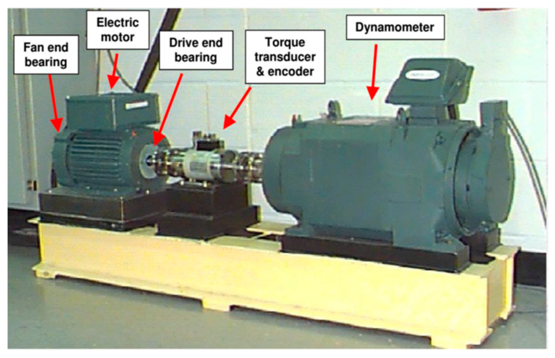
3. Brief Description of the CWRU Bearing Data Center Test Rig

The test rig used to acquire the Case Western Research University (CWRU) dataset consists of a 2 hp Reliance Electric motor driving a shaft, as shown in Figure 2. A torque transducer and encoder were mounted between the motor and the load (i.e., a dynamometer).

In order to study the response from damaged bearings, faults were seeded by electro-discharge machining (EDM) on the rolling elements and on the inner and outer races of the drive- and fan-end bearings (as described in

Table 1. Bearing fault frequencies details (BPFI/O: inner/outer race, FTF: cage, BSF: ball).

Location	Name	Fault Frequencies (Multiple of Shaft Speed)
		BPFI	BPFO	FTF	BSF
Drive End	6205-2RS JEM	5.415	3.585	0.3983	2.357
Fan End	6203-2RS JEM	4.947	3.053	0.3816	1.994

). These artificial damages ranged from 0.007 to 0.028 inches (0.18 to 0.71 mm) in diameter size. Three monoaxial accelerometers oriented along the vertical direction were placed on the housing of the drive-end bearing (DE), on the fan-end bearing housing (FE), and on the motor supporting base plate (BA). The acceleration signals were sampled at 12 kHz for some tests and at 48 kHz for others. The operational conditions were stationary in terms of speed, while two loads were applied: at 0 Hp the resulting motor speed was of 1797 rpm, while at 3 Hp it was reduced to 1720 rpm. The complete exploration of the whole database is out of the scope of this work; hence, a small selection of particularly relevant acquisitions [26] was selected, as summarized in

Table 2. Details of the selected acquisitions (DE: drive end, FE: fan end, IR: inner race, B: ball).

Name	Code	Acc. Location	Damage Location	Damage Size	Fs	Details
IR014_2	176	FE	DE-IR	0.014″	48 ksps	Good Acquisition
IR014_1	275	DE	FE-IR	0.014″	12 ksps	Impulsive noise
IR014_3	177	FE	DE-IR	0.014″	48 ksps	Electrical noise
B021_0	222	DE	DE-B	0.021″	12 ksps	Non-periodic impulses

. Their corresponding raw time series are reported in Figure 3. For further details refer to [32,33].

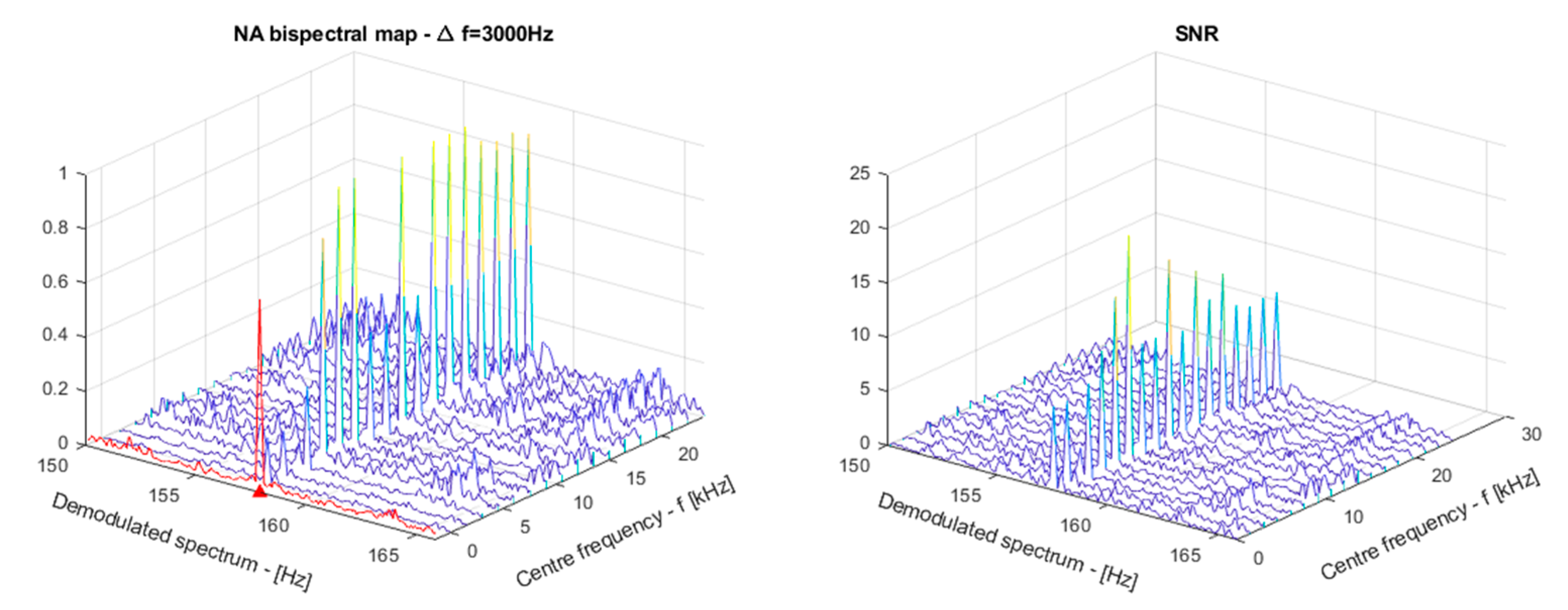
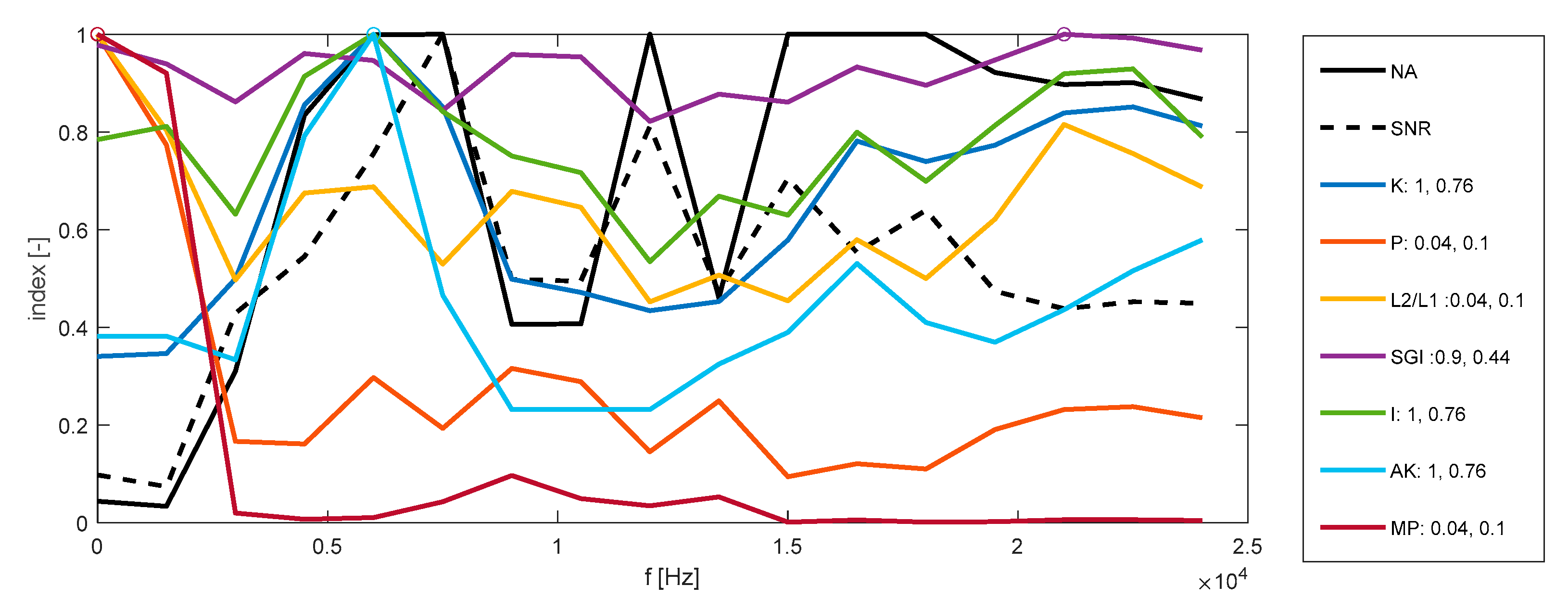
4. Results and Discussion

The methodology introduced in Section 2 was tested on the selected acquisitions reported in Table 2 so as to assess the effectiveness of the demodulation procedure (i.e., ease of detecting the defect frequency in the demodulated spectra) and the effectiveness of the different indicators in the selection of the optimal demodulation band according to the previously introduced dE and iE metrics. Note that according to [6], an order 16 FIR filter is used for the demodulation, while the Δf is set to 1/8 of the Nyquist frequency for all the acquisitions according to the consideration at the end of Section 2.

4.1. Acquisition IR014_2 (176FE)

Acquisition IR014_2 (176FE) was taken into account as it is a good and clean acquisition and can represent a case well in which it should be relatively easy to find a good demodulation band. In fact, the value of dE = 0.71 is quite high, as the demodulation is effective in most of the considered bands, as can be observed in Figure 4.

Once the exact characteristic frequency of the damage of interest f_d is established according to the procedure in Section 2, the section of the bispectral maps at f_d represent the NA and the SNR (i.e., the two proposed a posteriori indicators). It is now easy to compute the effectiveness of the different band indicators, whose frequency trend is shown in Figure 5. In the legend of the picture, the two ingredients of iE are in fact reported. Their average, which represents the indicator effectiveness according to Equation (11), are summarized in

Table 3. Summary of the results in terms of demodulation and indicator effectiveness.

Acquisition:		176FE	275DE	177FE	222DE	Avg
dE		0.71	0.59	0.58	0.18	-
iE	K	0.88	0.58	0.31	0.645	0.604
	P	0.07	0.79	0.615	0.235	0.428
	L2/L1	0.07	0.26	0.615	0.235	0.295
	SGI	0.67	0.26	0.06	0.645	0.409
	I	0.88	0.725	0.59	0.585	0.695
	AK	0.88	0.845	0.59	0.645	0.740
	MP	0.07	0.79	0.295	0.235	0.348

. For this particular case it is easy to notice that the spectral kurtosis (i.e., the indicator of the kurtogram, K), the average negentropy (I, the indicator of the infogram), and the indicator of the autogram (AK) show the best results, followed by the Spectral Gini Index (SGI). The protrugram indicator (P), the L2/L1 norm indicator (L2/L1), and the modified protrugram indicator (MP), on the contrary, had poor performance (even if in this simple case a weaker peak could be still found, as visible in Figure 4).

4.2. Acquisition IR014_1 (275DE)

Acquisition IR014_1 (275DE) was considered because it involves fan-end bearing damage (inner race fault), while the acquisition comes from the drive-end, so the demodulation should be more difficult. Furthermore, as can be observed in Figure 3, this signal involves transients leading to non-stationarities which should negatively affect the spectral kurtosis [26]. The higher difficulty in the demodulation is reflected by the dE = 0.59. Focusing on the resulting iE in Table 3, it is easy to see that in this case AK, P, MP. and I outmatch the spectral kurtosis K, which is better than L2/L1 and SGI. The corresponding indices as a function of frequency are reported in Figure 6a, where it can be noticed that not one of the indicators reach the optimal solution, but AK is the nearest.

4.3. Acquisition IR014_3 (177FE)

Acquisition IR014_3 (177FE) is corrupted by noise of an electrical nature around 0.5 s (refer to Figure 3). This anomaly seems to mainly affect SGI, MP, and K, while from Table 3 it is clear that I, AK, P, and L2/L1 can highlight the damage-characteristic frequency in quite an effective way. The spectral plot of the indices in Figure 6b highlights the presence of a single optimal band, but none of the indicators are able to precisely recognize it.

4.4. Acquisition B021_0 (222DE), Fan End Bearing Featuring Ball Fault, Non Periodic Impulses

Finally, Acquisition B021_0 (222DE) selected as the accelerometric signal is of a highly non-stationary nature, showing many large impulses. Regarding this, apart from MP, L1/L2, and P, all the other band indicators reported in Table 3 seem to be able to find a demodulation band which can produce good diagnostic results. From Figure 6c, it can be seen that in a large band (i.e., roughly 2000–4000 Hz) the envelope demodulation could lead to almost optimal results. Nevertheless, the best indicators (AK, K, and SGI) point to a suboptimal frequency range in the high-frequency portion of the spectrum. The result is suboptimal, but nonetheless acceptable from a diagnostic point of view.

5. Conclusions

Despite the number of analyzed acquisitions, this was not high enough to derive general rules. The proposed methodology seems to effectively allow the evaluation and comparison of the performance of the demodulation process itself, as well as the goodness of the band indicators traditionally used for bearing diagnostics. In fact, the paper proposes two novel a posteriori indicators, which were used for the computation of both a demodulation effectiveness metric and an indicator effectiveness metric.

From the results in Section 4, derived from a portion of the CWRU database, which, although reduced, considers many relevant signal peculiarities, it was possible to find a ranking of the considered band indicators. According to Table 3, by averaging the iEs in the four different cases, it was easy to notice how the autogram indicator AK proved to be very good for the selection of the optimal center frequency for the demodulation, as well as the averaged negentropy I, taken from the infogram. All of the other indicators, on the contrary, although only in some cases, appeared to behave better than the kurtogram indicator K, but not on average. This probably explains why the spectral kurtosis, the milestone for band selection, is still the reference algorithm for the bearing diagnostics.

Future improvements and applications may involve the definition of confidence intervals for the indicators [34], the application on different machineries and datasets such as in [35,36], the compensation of non-stationary rotational speeds [37,38,39], and the analysis of the effect of the sampling rate on the results.

The main limitation of this sort of “brute force” approach to the optimization is that it requires the computation of the SES in all the sub-bands, leading to longer computational times which prevent the use of such an algorithm in real time. Hence, further studies on the computational complexity and optimization of the algorithm could be conducted in the future.

References

1. Randall, R.B. Vibration-Based Condition Monitoring: Industrial, Aerospace and Automotive Applications, 3rd ed.; John Wiley & Sons: Hoboken, NJ, USA, 2011; ISBN 978-0-470-74785-8. [Google Scholar]
2. Randall, R.B.; Antoni, J. Rolling Element Bearing Diagnostics—A Tutorial. Mech. Syst. Signal. Process. 2011, 25, 485–520. [Google Scholar] [CrossRef]
3. McFadden, P.D.; Smith, J.D. Vibration monitoring of rolling element bearings by the high frequency resonance technique—A review. Tribol. Int 1984, 17, 3–10. [Google Scholar] [CrossRef]
4. Antoni, J. The spectral kurtosis: A useful tool for characterizing non-stationary signals. Mech. Syst. Signal. Process. 2006, 20, 282–307. [Google Scholar] [CrossRef]
5. Antoni, J.; Randall, R.B. The spectral kurtosis: Application to the vibratory surveillance and diagnostics of rotating machines. Mech. Syst. Signal. Process. 2006, 20, 308–331. [Google Scholar] [CrossRef]
6. Antoni, J. Fast computation of the kurtogram for the detection of transient faults. Mech. Syst. Signal. Process. 2007, 21, 108–124. [Google Scholar] [CrossRef]
7. Wodecki, J.; Michalak, A.; Zimroz, R. Optimal filter design with progressive genetic algorithm for local damage detection in rolling bearings. Mech. Syst. Signal. Process. 2018, 102, 102–116. [Google Scholar] [CrossRef]
8. Lei, Y.; Lin, J.; He, Z.; Zi, Y. Application of an improved kurtogram method for fault diag-nosis of rolling element bearings. Mech. Syst. Signal. Process. 2011, 25, 1738–1749. [Google Scholar] [CrossRef]
9. Barszcz, T.; JabŁoński, A. Analysis of Kurtogram performance in case of high level non-Gaussian noise. In Proceedings of the 16th International Congress on Sound and Vibration, Krakow, Poland, 5–9 July 2009. [Google Scholar]
10. Barszcz, T.; JabŁoński, A. A novel method for the optimal band selection for vibration signal demodulation and comparison with the Kurtogram. Mech. Syst. Signal. Process. 2011, 25, 431–451. [Google Scholar] [CrossRef]
11. Wang, D.; Peter, W.T.; Tsui, K.L. An enhanced Kurtogram method for fault diagnosis of rolling element bearings. Mech. Syst. Signal. Process. 2013, 35, 176–199. [Google Scholar] [CrossRef]
12. Peter, W.T.; Wang, D. The design of a new sparsogram for fast bearing fault diagnosis: Part 1 of “Two automatic vibration-based fault diagnostic methods using the novel sparsity measurement–Parts 1 and 2”. Mech. Syst. Signal. Process. 2013, 40, 499–519. [Google Scholar]
13. Wang, D. Spectral L2/L1 norm: A new perspective for spectral kurtosis for characterizing non-stationary signals. Mech. Syst. Signal. Process. 2018, 104, 290–293. [Google Scholar] [CrossRef]
14. Antoni, J. Cyclic spectral analysis of rolling-element bearing signals: Facts and fictions. J. Sound Vib. 2007, 304, 497–529. [Google Scholar] [CrossRef]
15. Antoni, J. Cyclic spectral analysis in practice. Mech. Syst. Signal. Process. 2007, 21, 597–630. [Google Scholar] [CrossRef]
16. Antoni, J.; Hanson, D. Detection of surface ships from interception of cyclostationary signature with the cyclic modulation coherence. IEEE J. Oceanic Eng. 2012, 37, 478–493. [Google Scholar] [CrossRef]
17. Antoni, J.; Xin, G.; Hamzaoui, N. Fast computation of the spectral correlation. Mech. Syst. Signal. Process. 2017, 92, 248–277. [Google Scholar] [CrossRef]
18. Wang, D. Some further thoughts about spectral kurtosis, spectral L2/L1 norm, spectral smoothness index and spectral Gini index for characterizing repetitive transients. Mech. Syst. Signal. Process. 2018, 108, 360–368. [Google Scholar] [CrossRef]
19. Miao, Y.; Zhao, M.; Lin, J. Improvement of kurtosis-guided-grams via Gini index for bearing fault feature identification. Meas. Sci. Technol. 2017, 28, 125001. [Google Scholar] [CrossRef]
20. Antoni, J. The infogram: Entropic evidence of the signature of repetitive transients. Mech. Syst. Signal. Process. 2016, 74, 73–94. [Google Scholar] [CrossRef]
21. Chen, X.; Zhang, B.; Feng, F.; Jiang, P. Optimal Resonant Band Demodulation Based on an Improved Correlated Kurtosis and Its Application in Bearing Fault Diagnosis. Sensors 2017, 17, 360. [Google Scholar] [CrossRef] [PubMed]
22. McDonald, G.L.; Zhao, Q.; Zuo, M.J. Maximum correlated Kurtosis deconvolution and application on gear tooth chip fault detection. Mech. Syst. Signal. Process. 2012, 33, 237–255. [Google Scholar] [CrossRef]
23. Borghesani, P. The envelope-based cyclic periodogram. Mech. Syst. Signal. Process. 2015, 58, 245–270. [Google Scholar] [CrossRef]
24. Smith, W.A.; Borghesani, P.; Ni, Q.; Wang, K.; Peng, Z. Optimal demodulation-band selection for envelope-based diagnostics: A comparative study of traditional and novel tools. Mech. Syst. Signal. Process. 2019, 134, 106303. [Google Scholar] [CrossRef]
25. Antoni, J.; Borghesani, P. A statistical methodology for the design of condition indicators. Mech. Syst. Signal. Process. 2019, 114, 290–327. [Google Scholar] [CrossRef]
26. Moshrefzadeh, A.; Fasana, A. The Autogram: An effective approach for selecting the opti-mal demodulation band in rolling element bearings diagnosis. Mech. Syst. Signal. Process. 2018, 105, 294–318. [Google Scholar] [CrossRef]
27. Daga, A.P.; Fasana, A.; Garibaldi, L.; Marchesiello, S. Fast Computation of the Autogram for the Detection of Transient Faults. In European Workshop on Structural Health Monitoring; Springer International Publishing: Cham, Switzerland, 2020; pp. 469–479. [Google Scholar] [CrossRef]
28. Kruczek, P.; Obuchowski, J. Modified Protrugram Method for Damage Detection in Bearing Operating Under Impulsive Load. In Cyclostationarity: Theory and Methods III; Springer International Publishing: Cham, Switzerland, 2017. [Google Scholar] [CrossRef]
29. Ho, D.; Randall, R.B. Optimisation of bearing diagnostic techniques using simulated and actual bearing fault signals. Mech. Syst. Signal. Process. 2000, 14, 763–788. [Google Scholar] [CrossRef]
30. Kim, S.; An, D.; Choi, J.-H. Diagnostics 101: A Tutorial for Fault Diagnostics of Rolling Element Bearing Using Envelope Analysis in MATLAB. Appl. Sci. 2020, 10, 7302. [Google Scholar] [CrossRef]
31. Borghesani, P.; Pennacchi, P.; Chatterton, S. The relationship between kurtosis- and envelope-based indexes for the diagnostic of rolling element bearings. Mech. Syst. Signal. Process. 2014, 43, 25–43. [Google Scholar] [CrossRef]