
Multi-Agent Reinforcement Learning: A Review of Challenges and Applications
by
 ,
,
Lorenzo Canese
†, 
Gian Carlo Cardarilli
, 
Luca Di Nunzio
†,
Rocco Fazzolari
†,
Daniele Giardino
†,
Marco Re
† and
Sergio Spanò
*,† Department of Electronic Engineering, University of Rome “Tor Vergata”, Via del Politecnico 1, 00133 Rome, Italy
*
Author to whom correspondence should be addressed.
†
These authors contributed equally to this work.
Appl. Sci. 2021, 11(11), 4948; https://doi.org/10.3390/app11114948
Submission received: 26 April 2021
/
Revised: 10 May 2021
/
Accepted: 24 May 2021
/
Published: 27 May 2021
(This article belongs to the Section Computing and Artificial Intelligence)
Abstract
:In this review, we present an analysis of the most used multi-agent reinforcement learning algorithms. Starting with the single-agent reinforcement learning algorithms, we focus on the most critical issues that must be taken into account in their extension to multi-agent scenarios. The analyzed algorithms were grouped according to their features. We present a detailed taxonomy of the main multi-agent approaches proposed in the literature, focusing on their related mathematical models. For each algorithm, we describe the possible application fields, while pointing out its pros and cons. The described multi-agent algorithms are compared in terms of the most important characteristics for multi-agent reinforcement learning applications—namely, nonstationarity, scalability, and observability. We also describe the most common benchmark environments used to evaluate the performances of the considered methods.
1. Introduction
In the field of machine learning (ML), reinforcement learning (RL) has attracted the attention of the scientific community owing to its ability to solve a wide range of tasks by using a simple architecture and without the need for prior knowledge of the dynamics of the problem to solve. RL has found uses in many applications, from finance [1] and robotics [2,3,4], to natural language processing [5] and telecommunications [6]. The core of a RL system is the agent that operates in an environment that models the task that it has to fulfill. In all of the above applications, the RL agents interact with the environment via a trial and error approach, within which they receive rewards (reinforcement) for their actions. This mechanism, similar to human learning, guides the agent to the improvement of its future decisions in order to maximize the upcoming rewards. Despite the success of this approach, a large number of real-world problems cannot be fully solved by a single active agent that interacts with the environment; the solution to that problem is the multi-agent system (MAS), in which several agents learn concurrently how to solve a task by interacting with the same environment [7]. In Figure 1, we show the representation of the RL structure for a single agent and for an MAS.
MASs can be used in several fields, for example, traffic control, network packet routing, energy distribution, systems of robots, economic modeling, and the analysis of social dilemmas. For these reasons, in the last few years, researchers have attempted to extend the existing single-agent RL algorithms to multi-agent approaches. Empirical evaluations, however, have shown that a direct implementation of single-agent RL to several agents cannot converge to optimal solutions, because the environment is no longer stationary from each agent’s perspective. In fact, an action performed by a certain agent can yield different rewards depending on the actions taken by the other agents. This challenge is called the non-stationarity of the environment and is the main problem to address in order to develop an efficient multi-agent RL (MARL) algorithm.
Even when convergence is obtained, typically, this kind of algorithm can maintain acceptable performance in terms of the quality of the policies derived and speed of convergence only if a restricted number of agents is involved. The scalability to a high number of agents is an essential feature that must be taken into account when developing algorithms that can be applied to real-world problems [8].
In this survey, we present an introduction to multi-agent reinforcement learning. We focus on the models used to the describe the framework environment and how to adapt the most relevant single-agent reinforcement learning techniques for multi-agent settings.
Below, we present an assortment of MARL algorithms that address the above-mentioned challenges of non-stationarity and scalability. We then address partially observable environments. For MAS, partial observability is far more common than in the single-agent setting; thus, it is crucial for the development of algorithms that can be applied to real-world problems. Finally, we introduce an overview of the most common benchmarking environments used to evaluate the performances of RL algorithms. This work is intended to be an introduction to multi-agent reinforcement learning, introducing the main challenges of the field and the main solutions adopted in the literature. Finally, we describe typical applications of MARL. While the research into MARL is still at an early stage and is often not supported by theoretical proof, it has shown promising progress in terms of its application. It could be considered a novel approach to achieve systems that are capable of helping humans perform complex tasks, such as working in hazardous environments, and exhibit general artificial intelligence.
2. Background
In the field of machine learning, reinforcement learning stands apart from the classic paradigm based on learning from examples. It adopts a trial and error procedure using a reward provided by an interpreter that observes the interaction of the agent with the environment. It takes inspiration from research into animal learning [9] combined with theoretical concepts of optimal control theory.
The interaction between the agent and the environment can be described by three fundamental elements: state, actions, and reward. The state represents a particular configuration of the environment, the actions are the options that the agents have to interact with to modify the environment, and the reward is a signal used to define the task of the agent and is what motivates the agent to pick one action with respect to the others.
The learning process is iterative. The agent senses the environment while collecting its current state. The agent performs an action, thereby reaching the next state, and it receives a reward based on the combination of the state and selected action. This process is then repeated. The agents adopt a policy to determine the best action to select, which is a mapping from all the possible states of the environment to the action that can be selected.
The reward, however, is not sufficient to determine the optimal policy because an instantaneous reward does not give information about the future rewards that a specific action can lead to—that is, the long-term profit. For this reason, it is useful to introduce a new kind of reward: the return value . If we write as the reward received by the agent at the time-step t, the return value over a finite length time horizon T is defined as
Sometimes, the return value is also considered for non-finite time horizons.
where is a discounted factor such that . To evaluate the quality of a particular state or state–action pair, it is possible to define two value functions. In particular, under a policy , the value function of the state is calculated as
and the value faction of the state–action pair is calculated as
A value function can be expressed as the relation of two consecutive states and defining the so called Bellman Equations (5) and (6).
and
A way to approximate the solutions to these equations is by using dynamic programming. However, this approach requires complete information about the dynamics of the problem. Model-free RL algorithms can be considered as an efficient alternative.
2.1. Multi-Agent Framework
Before introducing the algorithms used in RL, we present the most used frameworks for modeling the environment of such applications. We begin with the single-agent formulation and then extend the concept to multiple agents.
2.1.1. Markov Decision Process
In the single-agent RL, the environment is usually modeled as a Markov decision process (MDP).
Formally, a Markov decision process is defined by a tuple , where
- S is the state space;
- A is the action space;
- is the transition probability from state to given the action ;
- is the reward function, whose value is the reward received by the agent for a transition from the state–action pair to the state ;
- is the discount factor and is a parameter used to compensate for the effect of instantaneous and future rewards.
2.1.2. Markov Game
When more than one agent is involved, an MDP is no longer suitable for describing the environment, given that actions from other agents are strongly tied to the state dynamics. A generalization of MDP is given by Markov games (MGs), also called stochastic games. A Markov game is defined by the tuple , where
- is the set of agents;
- S is the space observed by all agents;
- is the action space of the i-th agent and is called the joint action space;
- is the transition probability to each state given a starting state and a joint action ;
- is the reward function of the i-th agent representing the instantaneous reward received, transitioning from to ;
- is the discount factor.
2.1.3. A Partially-Observable Markov Decision Process
A partially-observable Markov decision process (POMDP) is a generalization of an MDP that considers the uncertainty regarding the state of a Markov process, allowing a state information acquisition [10]. We can define a POMDP using two stochastic processes: the first is a non observable core process that represents the evolution of the state and is assumed to be a finite state Markov chain; the second is an observation process that represents the observations received by an agent. There is a probabilistic relationship between and that links the probability of observing a particular value of if the agent is in the state .
A POMDP is well suited to modeling a large variety of RL problems even though it is an intrinsically more complex method than using an MDP.
2.1.4. Dec-POMDP
A decentralized partial-observable Markov decision process (Dec-POMDP) is defined by the tuple , where
- I is the set of n agents;
- S is the state space;
- is the joint action space;
- is the observation space with .
The state S evolution is based on the transition probability . It indicates the probability that, given the joint action and the current state s, the next state will be . At every time step, all agents receive an observation given by the joint observation probability . For each agent i, we can define its local observation history at iteration t as , where . At every iteration, the team receives a joint reward conditioned by the joint action and the current state. This is used to maximize the expected return over the horizon T where is the discount factor [11]. As in the Markov games framework, the objective is to maximize the expected return by selecting an optimal joint policy. However, in this case, the policy performs a mapping from local observations to actions; thus, we can write the local policy of agent i as .
2.2. Single-Agent RL Algorithms
The field of RL is extremely broad, and over the last few years, a multitude of algorithms have been presented. To categorize them, the first division can be made between model-free and model-based algorithms. Model-based algorithms require users to have access to a model of the environment, including the transition probability and the associated reward, or to learn the model directly during training. They then use the model to plan the best action to take. An example of this approach is the DYNA algorithm [12]. This approach leads to an optimal solution; however, in most applications, a model of the environment cannot be obtained or would be too complex to implement. Moreover, the quality of the solutions is sensitive to error in the model estimation. Another downside is a loss of computational efficiency in cases in which the model is highly complex but the optimal policy is very simple. An example could be a complex robotic system that has to learn only how to move forward. In recent research, the efficiency of the learned model has been addressed, obtaining state-of-the-art performances with approaches such as MuZero and AlphaZero [13,14].
Model-free algorithms do not require any knowledge about the model, and they operate by directly optimizing the policy or other value parameters. This type of approach is goal-oriented and can perform in a variety of environments and adapt to their changes. In this work, we focus exclusively on model-free algorithms. Model-free algorithms can be further divided in two fields: value-based approaches and policy-based approaches.
The objective of value-based methods is to find good estimates of the state and/or state–action pair value functions and . The optimal policy is selected using a fixed rule to map from the value functions to the actions; for an example, take the policy, which selects the action associated with the higher Q-value with probability and a random action with probability . An example of this approach is the famous Q-learning algorithm [15]. Policy-based methods do not require the value function to be estimated but use a parameterized policy that represents a probability distribution of actions over states as a neural network. The policy is directly optimized by defining an objective function and using gradient ascent to reach an optimal point. If we consider, for example, the reward as the objective function, we can derive the expression
which is known as the policy gradient theorem. While the expected value of the reward cannot be differentiated, the policy can, making gradient ascent possible. A last category of RL algorithms that originates from the combination of policy-based and value-based methods is the actor–critic approach. As shown in Figure 2, in an actor–critic algorithm, two different learning agents are defined:
- The critic, which has the task of estimating the value function, typically using TD methods;
- The actor, which represents the parameterized policy and updates its action distribution in the direction "suggested" by the critic using a policy gradient.
The critic outputs a signal that changes the action selection preferences in order to chose actions related to higher value functions more frequently. This kind of algorithm presents a reduced variance in the gradient estimates due to the use of the value function information to guide the policy evolution. In addition, minimal computation is required to select an action as there is no need to compare different state–action values, and it is possible to learn an explicitly stochastic policy [16].
All of these methods, as summarized in Figure 3, have been used with success in the solution of RL problems, and their effectiveness is dependent on the type of problem.
2.2.1. Q-Learning
Q-learning [15] is a form of model-free, value-based reinforcement learning. It takes inspiration from dynamic programming and methods of temporal differences such as TD(0) [17]. The Q-learning agent faces the task of determining an optimal policy that maximizes the total discounted reward; this policy is such that
where is the average reward received by an agent in the state s if it selects the action a, and is the transition probability from the state s to , given the action a. The object is to estimate the state–action pair value function (Q-values); this is done by creating a matrix of dimensions containing the estimates of all the value functions at the time-step n. At each iteration n of the learning process, the Q-values are updated using the equation
where is the learning rate, is the instant reward received, and
It was shown in [18] that, under the assumption of bounded rewards and learning rates such that
the estimates will converge to the optimal Q-value with probability 1.
2.2.2. REINFORCE
REINFORCE is a class of episodic reinforcement learning algorithms that have the most simple implementations of the policy gradient methods; for this reason, the name vanilla policy gradient exists [19]. The policy is directly optimized without the need to estimate the value functions. The policy is parameterized with a set of weights such that , and it is the probability distribution of actions over the state. Regardless of the architecture of the parameterized policy, all REINFORCE algorithms use the same weight update procedure:
where is a non-negative learning parameter, is the discounted return value, and b is the baseline, which is used to reduce the variance of the gradient estimation. b is a function of the state (a constant without loss of generality). The steps to implement a REINFORCE algorithm are the following:
- Initialize the policy parameters at random;
- Use to generate a trajectory, which is a sequence of states, actions and rewards, ;
- For each time-step ,
- Estimate the return ;
- Update policy parameters using Equation (12);
- Iterate the process.
2.2.3. A3C
Recalling the policy update rule of REINFORCE , a frequently used baseline b is a learned estimate of the state value function . If this kind of baseline is selected, we can express the term as an advantage function because is an estimate of the state-action value function. This approach can be viewed as an actor–critic method in which the actor is the policy network and the critic is represented by the baseline. In [20], A3C (asynchronous advantage actor critic) and its synchronous variant A2C are presented; the algorithm maintains a policy function parameterized by and an estimate of the value function parameterized by . In the formulation, the weights are considered separately; in the implementation, the same deep convolutional neural network is used to approximate the policy and the state value, with the only difference being in the separated output layers (a soft-max layer for the policy and linear layer for the state value). The algorithm continues for a number of steps or until it reaches a terminal state; the return value is then calculated, and the updating of the parameters is performed following the gradient. In Algorithm 1 the psuedocode of the A3C algorithm can be found.
The algorithm was trained and tested in a variety of domains, such as the Atari 2600 platform, improving upon the results of state-of-the-art RL algorithms such as the Deep Q-network [21].
| Algorithm 1 A3C Pseudocode [20]. |
|
3. The Limits of Multi-Agent Reinforcement Learning
MARL algorithms can be coarsely divided into three groups depending on the kind of reward given by the environment: fully cooperative, fully competitive, and mixed cooperative–competitive. In the cooperative setting, all the agents collaborate to maximize a common long-term return. An example of this setting is a smart energy grid, in which multiple buildings (agents) with different energy production capabilities have to share energy in order to minimize the outside-grid energy demands. Another is an autonomous driving setting in which the vehicles have to collaborate in order to avoid collisions while trying to maximize traffic flow and possibly fuel efficiency. In competitive settings, the return of all the agents sums to zero. A variety of board and card games, including chess, Go, and poker, belong to this setting, and are of great interest in the reinforcement learning community as benchmarks for algorithms. Mixed settings combine the aforementioned characteristics and present a general-sum reward; a typical example of this is constituted by team games in which the agents have to cooperate with their own team-mates while competing with the opposing teams. The transition from single-agent to multi-agent settings introduces new challenges that require a different design approach for the algorithms.
3.1. Nonstationarity
The environment in a multi-agent setting can be modified by the actions of all agents; thus, from the single-agent perspective, the environment becomes non-stationary. The effectiveness of most reinforcement learning algorithms is tied to the Markov property, which does not hold in non-stationary environments [16]. Policies created in a non-stationary environment are deemed to have become outdated. Despite the loss of theoretical support, algorithms designed for the single-agent setting have been applied in multi-agent settings, such as independent learners (IL), occasionally achieving desirable results [22]. A naive approach to tackle the non-stationarity is the use of joint action learners (JAL). This uses a single-agent RL but with the joint action instead of the local action used to compute its value functions. This approach eliminates the problem of non-stationarity entirely; however, it is computationally ineffective, and the action space dimension becomes , where N is the number of agents, making it difficult to scale this type of approach to more than a few agents. In addition, to ensure that every agent knows the actions of others, some type of centralized controller or communication network is required [23]. In [24], a variation of Q-learning for swarm systems is presented, called Q-RTS. The key idea is to use a centralized aggregation center to combine all the Q-value tables of the agents to form a global swarm matrix containing the highest and lowest Q-values representing the most interesting iterations by the agents. The swarm matrix is then linearly combined into the local Q-value matrix of each agent using an independence factor , controlling the tradeoff of local and global knowledge. The Q-learning update then proceeds independently on for each agent.
An FPGA implementation was also proposed [25].
Varying Learning Speed
The effect of environmental non-stationarity is to make the reward information of state–action pairs related to past iterations obsolete, and this effect grows as time progresses. Several approaches tackle this challenge by adopting varying learning rates with the aim of guiding the training to the most efficient joint policy. In the context of cooperative games, hysteretic Q-learning [26] is an algorithm that improves the performance of standard independent learners approaches. The reward is shared between agents and conditioned by the joint action; thus, an agent can be punished even if it select the optimal option due to the bad actions of other teammates, who might be exploring. The algorithm applies a different learning rate if the update would cause a decrease of the Q-value using the update Equation (15) under the condition that .
This heuristic has the positive effect of implementing "optimistic" agents that are able to ignore the bad rewards caused by the actions of others, improving the performance compared to traditional IL approaches in cooperative MGs. In [27], the authors argue that in order to obtain robustness against incorrect future reward estimation, in the early iterations of the reinforcement learning algorithms, the agents need to show some sort of leniency towards others. In particular, the future reward for a performed action can be assessed as the maximum reward received over a number of different actions chosen by the other agents. The proposed algorithm is called lenient multi-agent reinforcement learning (LMRL) and implements varying leniency, lowering the amount that each agent exhibits in the later stages of learning. Agents decide the amount of leniency to apply by associating a temperature with each state–action pair. The level of leniency is inversely proportional to the temperature and decreases as those state–action pairs are selected.
3.2. Scalability
As the number of agents increases, there is a growth in the joint action space. For this reason, centralized approaches, in which an observer selects the actions after receiving the action–state information of every agent, require large amounts of computational resources and memory to work with more than a couple of agents. A possible solution to the curse of dimensionality in MARL is to use independent learners, but as we have seen, this approach is unable to obtain consistent results in a non-stationary environment. A third model of agent connection is the decentralized setting with networked agents. In this setting, every agent is able to interact with the environment and to exchange information with few other agents (typically, those in its vicinity), creating a time-varying communication network between all the agents. Algorithms developed for this setting are scalable to a massive number of agents and more real-world-oriented applications, as the absence of a central controller and uncertainty in communication links are typical requirements in a large number of applications. In [28], a distributed version of Q-learning, namely, QD-learning, is proposed under the assumption that each agent is only aware of its local action and reward and the inter-agent communication network is weakly connected. The optimal policy is achieved by agents sending their Q-values to their neighbors. The update of the Q-value is then computed locally for each agent using the following equation:
In can be seen from Equation (16) that the update is defined by two processes, consensus and innovation, where the former is the sum of the differences of the Q-value of the agent and the Q-values of its neighbors, controlled by the weight sequence , and the latter is the traditional Q-learning update rule weighted by the sequence . In [29], the same setting of decentralized reinforcement learning with networked agents is addressed using an actor–critic algorithm. The policy is parametrized by a set , and the gradient of the globally averaged return with respect to is given by
The local advantage function is defined as
where and is the action chosen by every agent except for agent i. The advantage function is not available considering only local information, so is estimated with the state–value TD-error, which is an unbiased estimator of the advantage function.
Deep Reinforcement Learning
Function approximation is a common technique for reducing the number of parameters in high-dimension state–action spaces. The use of a deep neural network to approximate the state–action value function, called deep reinforcement learning (DRL), was first presented in [21] in the single-agent setting and achieved promising results in the training of an agent capable of playing a large set of Atari 2600 games using the raw pixel data from the screen as the input for training. The success of the proposed approach is based on two features. The first is the introduction of an experience replay mechanism in which every experience tuple , composed of the state transition, action selected, and reward received, is stored in a dataset and then randomly batched to train the action–value approximation network. This method eliminates the correlation between consecutive iterations, which is inevitable for sequentially generated data points. The experience replay also has the additional effect of increasing the sample efficiency by reusing experience tuples. The second feature is the use of two networks to approximate Q, the Q-network, and the target network; the parameters of the latter are updated every C steps with the Q-network parameters and used as the target of the training loss function, defined as
in which is the discount factor; and are the parameters of the target network and of the Q-network at iteration i, respectively. Policy gradient methods have been extended to make use of deep neural networks, keeping the advantage of allowing for policies in the continuous action space. In [30], a deep Q-network was combined with an actor–critic approach. The parameterized actor that represented the policy and the critic that estimated the value using the state–action pair were represented by DQNs. The networks were trained using a deterministic policy gradient algorithm with a batch normalization technique [31]. The performances obtained have motivated the research community to adopt deep networks in the multi-agent environment. In [32], the lenient reinforcement learning algorithm was adapted to DRL, and the authors thus proposed the lenient deep Q-network (LDQN) algorithm. In [33], the authors proposed two techniques to stabilize the effect of the experience replay in the multi-agent setting: low-dimensional fingerprints, made by a Boolean vector, were added to the experience tuple to disambiguate training samples; and importance sampling, which consists of recording the other agent policies in the experience replay, forming an augmented transition tuple . The DQN parameters are trained by minimizing the importance-weighted loss function analogous to Equation (19).
where b is the size of the batch used in the learning and is the output of the target network.
3.3. Partial Observability
Most of the algorithms presented are based on the assumption of the full observability of the state by all agents. In most real-world applications, this condition is rarely present, as agents observe different instances of the state; for example, an agent may have vision of only its surroundings, making the observations correlated with its geographical position, or the agents might be provided with different sets of sensors. In the setting of DRL, the algorithms developed for the full state can only achieve desired performance if the observations are reflective of the hidden system state. In [34], an algorithm called the deep recurrent Q-network (DRQN) was proposed. The first layer of the DQN was replaced with recurrent long short-term memory (LSTM). This architecture was tested on flickering versions of Atari games in which the state (the pixels of the game screen) was sometimes presented to the agent and sometimes obscured. In this benchmark, DRQN achieved better performance than the traditional DQN. This idea was transferred to the multi-agent setting in [35], which integrated hysteretic learning [26] to deal with the non-stationarity of the environment and the capabilities of representing the hidden state space of deep recurrent Q-networks, proposing an algorithm called the decentralized hysteretic deep recurrent Q-network (Dec-HDRQN). In the work, a variation of the experience replay mechanism called concurrent experience replay trajectories (CERTs) was used. In CERT, each experience tuple containing the current observation, action, and reward, and the subsequent observation, is indexed by the agent number, the time-step of acquisition, and the episode. The samples given to the Q-network for training are then taken from this structure in a synchronized way.
3.3.1. Centralized Learning of Decentralized Policies
Scalability and partial observability are connected problems, especially when considering the applications of algorithms to real-world problems. In a setting with an extremely high number of agents, as in the case of the number of autonomous driving cars in a city, it is impossible for every car to have full information about the state, as cars cannot exchange information with each other without a prohibitive communication overhead. The full information about the state could therefore not be useful for executing an optimal policy, but it could be useful during the learning phase to correctly estimate the value-functions or the policy gradients. To exploit this dichotomy, the paradigm of centralized learning of decentralized policies was introduced. The idea behind this is that, during learning, it is often possible to have access to a simulator of the environment or a central controller, or have additional information about the state. We can imagine a setting in which the agents are, for example, a swarm of drones trained in a closed building, such as a hangar, with limited visibility, and the extra information about the state of the environment is given by a fixed camera looking down on all of the drones. In [36], a comparison between various training schemes—centralized, independent learning, and centralized training—for decentralized policies using parameter sharing is presented. A parameter sharing variant of the single agent algorithm trust region policy optimization (TRPO) [37], namely, PS-TRPO, is presented. The decentralized paradigm obtained the best performance of all the training schemes in the evaluation phase. In addition, the scalability of the PS-TRPO algorithm was addressed using curriculum learning [38], in which the agents had to solve a number of sub-tasks that increased in difficulty in order to coordinate with an increasing number of agents. To exploit the utility of having a centralized learning phase in [39], a novel actor–critic architecture, called the conterfactual multi-agent policy gradient (COMA), was presented. In the training, a single centralized critic is used, which estimates the Q-function using the joint action and the full information on the state, or in the absence of a well-defined state, the concatenation of all the local observations made by the agents, and several decentralized actors that deploy a policy which maps from local observations to an action. Additionally, COMA tackles the challenge of multi-agent credit assignment in a cooperative setting where there is a unique reward shared to all the agents. Training is more efficient if each agent is able to determine how an action reflects on the success of the task. This is done through the use of a counterfactual baseline; each agent receives a shaped reward, which is the difference between the reward obtained at the time-step t and the reward that would be obtained if the agent actions were to change to the default . It can be shown that any action by the agent a that improves also improves the true global reward. The main downsides of this approach are the necessity for a simulator of the environment to calculate and the choice of the default action , which is not always trivial. Both of these problems were addressed by the architecture of the critic which computed for each agent an advantage function as follows:
In particular, the actions are given as an input to a network that determines the state–action value for each action of the agent a in a single forward pass.
| Algorithm 2 COMA pseudocode [39]. |
|
This algorithm (full pseudocode can be found in Algorithm 2) was tested in Starcraft, a combat-based video-game environment. Several homogeneous and heterogeneous unit combinations, with each one represented by an agent, were considered. It was shown that, in that setting, COMA reached competitive performance in regard to fully centralized methods with better training speed. While the paradigm of the centralized learning of decentralized policies is easily implementable for actor–critic and policy gradient methods, it is not as straightforward when considering value-based methods. A possible approach was presented in [40] that consists of decomposing the team value function into agent-wise value functions. The assumption on which this approach is based is that the joint action–value function can be factorized according to each agent’s Q-function based only on each agent’s local observation:
Each agent taking a greedy action to maximize their returns is equivalent to a central controller maximizing the joint action–value functions. The value decomposition network (VDN) used DQN or DRQN, with the possibility of communication between agents at a low level (sharing observations) or high level (sharing network weights). It was tested in a two-dimensional grid environment, obtaining better performances than the centralized and independent learners methods. The limit of this approach is that not every multi-agent problem can be approximated and solved as a summation of Q-functions. In [41], the VDN method was extended with the QMIX algorithm. The authors argued that a full factorization of the value function is not required to extract effective policies. It is sufficient that the result of an on the joint action–value functions produces the same result to apply an to all the individual action–value functions. This is possible if a monotonicity constraint is enforced between the total Q-value and local agent Q-value .
Each agent value function is represented by a DRQN that takes, as its input, the local observation and the last action at each time step. Then, the singular value functions are combined using a mixing network, which is a feed-forward neural network. The weights of the mixing network are bounded to be non-negative to enforce the condition presented in Equation (23). These weights are determined by a separate hyper-network which takes the augmented state as its input. The networks are trained to minimize the loss function in a way analogous to DQN:
with transitions sampled by the replay buffer. In the evaluation carried out in the StarCraft II Learning Environment, QMIX obtained better results than VDQ at the cost of the added architectural complexity. VDQ combines the local Q-functions using a simple summation, whereas QMIX uses a neural network.
3.3.2. Communications between Agents
In the case of the partial visibility of the environment, the use of communication between agents is often a necessity, as collaborating agents can then better infer the underlying state of the environment. Communication protocols are often hand-designed and optimized for the execution of particular tasks. In contrast with this approach, in [42], a simple neural communication model called CommNet was proposed, which learned a task-specific communication protocol that aided the performance of the agents. Considering a setting with J fully cooperative agents, a model was proposed with , where is the concatenation of discrete actions for each agent j and is the concatenation of all agents observations. is built from modules consisting of a multi-layer neural network with , where K is the number of communication steps of the network. Each agent j sends two input vectors to the module—the agent’s hidden state and the communication , and outputs the next hidden state . The evolution of the hidden space and the communication message is regulated by the following equations:
The first hidden state is obtained through an encoder function , which takes the state observation of agent and outputs its hidden state. is made of a single layer neural network. After the last round of communication, a decoder function, made of a single layer neural network followed by a softmax, is used to convert the hidden state to a probability distribution over the space of action . The action is chosen by sampling this distribution. A variance of the broadcast transmission represented by Equation (26) is a local connectivity scheme:
where is the neighborhood of agent j.
This model was tested with various difficult tasks, including a traffic simulation with four connected crossroads, with the objective being to avoid collisions while trying to maximize the vehicle flow. Promising results were obtained even with a very limited—if not absent—observability of the state. Another similar work addressing the communication problem in a multi-agent partially-observable setting was presented in [43] using a deep distributed recurrent Q-network (DDRQN) architecture. This approach takes inspiration from the single-agent DRQN algorithm [34] and generalizes it to a MA setting by making three fundamental modifications: Last-action inputs—giving each agent access to its previous action as an input for the next time-step; inter-agent weight sharing—a single network is learned causing a quicker learning process. Weight sharing allows diverse behavior between agents, as the agents receive different observations and thus evolve in different hidden states; disabling experience replay—this modification is made as the non-stationarity of the environment renders old experiences obsolete or misleading. As a proof of concept, this architecture was used for the solution of two multi-agent reinforcement learning problems based on the well known riddles of the hat riddle and the switch riddle. In these problems, the optimal solution can only be achieved if the agents reach a consensus on a communication protocol to use to solve the task. In Table 1, a summary of all the presented algorithm can be found with a brief explanation of its principal features and their scientific spreading. The latter was evaluated according to the number of search results from the Google Scholar indexing service. In Figure 4, a summary of all the algorithms with regard to the challenges they address is presented.
4. Benchmark Environments for Multi-Agent Systems
Reinforcement learning, especially when compared to more traditional data-driven machine learning approaches, presents an implicit difficulty in terms of evaluating the performance of its algorithms. For small problems, it is possible to compare the obtained policies to optimal ones computed using, for example, game theory. The performance is evaluated as the number of steps and/or episodes required to converge at the optimal policy. When the state and actions space grow in size—for example, due to the introduction of multiple agents—the optimal solution gradually becomes intractable, and this type of approach cannot be used. Since reinforcement learning uses an online, experience-based approach to learn policies with data generated by a simulator or by in-field implementation, it is a natural fit to use the same infrastructure during the evaluation phase to determine the effective performance of the algorithm. There are two main types of environments used to evaluate the performances: continuous and episodic-based simulation. In a continuous simulation, the agents act in an environment that is capable of generating tasks for a theoretical infinite time horizon, and the performances can be represented as the sum of cumulative rewards over a fixed time-step window. This could apply to a traffic simulation in which the performances are determined by the number of total collisions in a fixed time slot. On the other hand, episodic-based simulations are characterized by a number of final states that represent the completion of a task and a maximal time-step at which the system reaches a terminal state, indicating that the task has failed. In this case, a possible benchmark could be to run a number of episodes and present the percentage of completed tasks over the number of simulated episodes.
MazeBaze [44] is a highly configurable, open source, 2D learning environment that is suitable for cooperative and competitive tasks. The environment is represented by a rectangular grid in which a set of items is placed; these items could be obstacles, goal grids, movable objects, doors, and switches, granting a flexible approach for task definitions.
MazeBaze was developed for single-agent environments but is easily adapted to multi-agent scenarios, as was performed in [42] to create a traffic junction, as shown in Figure 5. The environment can be sensed by the agents as a set of features or directly using the pixel representation of the environment as an input. Another useful framework to evaluate the decision making and coordination capabilities of a group of agents is the strategic video-game Starcraft—in particular, the Starcraft II Learning Environment (SC2LE) [45], which is a combat-based learning environment that allows the development of algorithms with heterogeneous agents with partial observability. The difficulty of the problem makes it a good benchmark for cooperative multi-agent algorithms. If the end-goal of the algorithm is to develop robotic movement control, the physics-based environment of MuJuCo [46] is ideal. This environment offers some robotics-related features, such as the avoidance of joint violation and the capability to operate in continuous action spaces.
5. Applications
MARL algorithms have been used in a variety of applications in different fields thanks to their ability to model competitive and cooperative scenarios. In [47], a team of UAVs equipped with a downward-facing camera was considered; the UAVs were assigned the task of optimal sensing coverage. The drone fleet had to cover an area of interest under its FOV while minimizing the overlap between camera captures. This task is required in several applications, such as wildlife monitoring or search and rescue, where the use of UAVs is growing due to their mobility and ease of deployment. UAVs are considered as independent agents, and the convergence to a singular joint action policy is obtained by the means of social conventions. The agents act in a prior-defined order so that the last agent can observe the preceding actions of its teammates and make a decision accordingly. This action selection order allows easy collision avoidance, as the agents are not able to choose an action that will cause a collision with its predecessors. To emphasize collaboration between agents, a single global reward is used during learning, and to reduce the dimensionality of the state space, several techniques of function approximation are implemented. In [48], the authors proposed a novel actor–critic multi-agent reinforcement learning algorithm to address the problem of multi-UAV target assignment and path planning (MUTAPP). A team of UAVs operates in an environment containing target locations to reach and locations to avoid and has to decide the most efficient way to maneuver while avoiding collisions. The critic and the actor are designed according to the multi-agent deep deterministic policy gradient (MADDPG) algorithm [49]. The critic of each agent shares its actions and observations during training while the actor network works exclusively based on local information. The reward signal is factorized into three components, with each one being responsible for a desired behavior: minimizing travel distance, avoiding collisions with other agents, or avoiding collisions with target areas. The evaluation was performed using the openAI platform and showed that the proposed algorithm can solve the problem of MUTAPP. In terms of convergence speed over the number of agents, the method showed some evident limitations in scaling.
Another UAV application used a UAV team to implement a network for line-of-sight (LoS) communications using MARL to optimize resource management, including the transmit power and subchannel selection [50]. The multi-agent setting is addressed via independent learner agents using Q-learning to maximize the future rewards, defined as the difference between the data throughput and the cost of power consumption. Agents select an action tuple where is the selected user, is the selected subchannel and is the power level. A simulation showed that, in this context, if a high exploration level is selected ( = 0.5), the algorithm can reach a tradeoff between system performance and information exchange that other methods in this setting require, such as the Gale–Shapley algorithm, which is based on the matching theory for user selection [51]. In [52], the authors study the problem of the limited spectrum in UAV networks considering a relay-based cooperative spectrum leasing scenario. The UAV fleet needs to transmit its data to a fusion center and does that by forwarding data packets for a ground user in exchange for spectrum access. The objective of the algorithm is to partition the UAVs into two groups: the relaying group, which handles the data transfer for the ground user, and the transmitting group, which forwards packets to the UAV fusion center. The learning algorithm is developed in a distributed way using independent learner agents using Q-learning without the need for communications, but only has access at the task partition, which serves as the state (we can consider this to be a fully observable setting). The algorithm was tested in scenarios with two UAVs and six UAVs and in both cases managed to achieve the optimal configuration.
In [53], a multi-agent approach based on a CommNet architecture [42] was proposed to coordinate the operation of the wireless recharging towers of a group of UAVs. The aim of the algorithm was to schedule the UAV to serve, determine how much energy should be delivered, and share the energy between charging towers. Each tower had access to a local photo-voltaic power generator, and the energy was shared to minimize the purchase of electricity from the energy market, resulting in lower operating costs. The proposed algorithm was tested in an urban simulation consisting of 30 UAVs and four charging towers. It performance improvements over the baseline policies of random sharing and scheduling.
Applications of MARL do not consider only the control of UAV fleets. In [54], the problem of a joint top-down active search of multiple objects was addressed. Each detector was an agent, and deep reinforcement learning was used to learn the optimal policy for object localization. Coordination between agents was obtained by the use of a differential message for each agent, which was a function of the action selected and the state of the environment with parameters , . The agent-wise Q-function was then defined as
The agent could control the effect of messages from other agents in its decision making process by the use of a learning gating mechanism. The algorithm was tested with a two-agent implementation on a series of datasets for joint image detection of man–bike, ball–racket, or person–handbag; the joint model achieved good performance using fewer iterations than the single-agent counterpart. Agents managed to "help" each other by sending clues about the correlations between object locations in the messages. In [55], a deep multi-agent reinforcement algorithm was developed to regulate the energy exchange between a community of buildings with heterogeneous energy production and storage capabilities. The objective was to reach nearly zero energy community (nZEC) status, which is defined as "A micro-grid that has distributed generation, storage, delivery, consumption and zero net annual energy balance." The buildings were modeled as DRL agents, and the authors proposed the presence of a community monitoring service (CMS) to aggregate data from all the agents and enable cooperation. Each agent used its local energy generation, consumption, and storing states as its states, and the energy balance of the entire community. This information was used to select an optimal action, maximizing the global reward signal given by the CMS, which was the negative of the community energy status
where is the energy consumed by the i-th house and is the energy generated by the i-th house. This approach was tested in a simulation of a summer and winter setting with up to 10 agents and confronted with some behavioral baselines, including never-share, always share and a random selection of actions. Baselines were outperformed especially in the summer setting. A limitation of this approach is that the learning was conducted using an episodic base approach and thus there is no guarantee that using an online learning approach would lead to the same convergence to an optimum.
In [56], a novel multi-agent reinforcement learning algorithm called Equilibrium selection MARL (ES-MARL) to control the energy scheduling of residential microgrid was presented. The microgrid consisted of renewable energy generators (RG) (wind turbines and photo-voltaic), households that demanded energy from the grid and a number of electric vehicles (EV) that could offer or request energy when connected to a recharging station with a Vehicle to Grid (V2G) connectivity. The algorithm uses several types of agents: an EV Aggregator agent that macromanages the exchanges of energy of all the EVs parked by demanding a certain charging power from the grid or by offering power to the grid while selecting the price; a User Aggregator agent, which receives the energy demand of the residential household and decides how much load to curtail (i.e., reducing air conditioning) and how much load to shift to another time-step (i.e., postponing the use of a washing machine). Two RG agents—one for each type of energy generation—were used to decide the price for selling their energy production. Cooperation between the heterogeneous agents is achieved throughout the action of an Equilibrium Selecting Agent with the objective of separately negotiating with all the agents to select the optimal equilibrium based on the average reward. Several scenarios of the microgrid were simulated, and the proposed approach showed an higher average reward compared to single-agent reinforcement learning approaches. When confronted with another MARL algorithm, such as Nash-Q [57], ES-MARL showed a faster convergence rate.
A similar application but for an industry production control setting was presented in [58]. An independent MARL algorithm based on Proximal Policy Optimization (PPO) was proposed to control the energy exchanges in a factory, composed of local power generators (renewable and fuel based), a battery system and a certain number of resources that could consume power to produce a variety of products. Each of these elements were represented in the algorithm as separated agents and a market agent that regulated the energy purchase from the energy market. The coordination between agents was encouraged by the use of a global reward combined with agent-specific local rewards. The reward function could be decomposed into energy and production costs that needed to be minimized. The proposed algorithm was compared to a reactive control strategy (RCS) and a predictive–reactive control strategy (PCS). MARL outperformed the RCS but did not match the performance of the PCS, indicating that it was able to reach only a local optimum. Comparing the time required to make a decision ( 1 s for MARL and 2.5 h for PCS), the MARL approach showed the capability to operate online and change its policy in real-time according to stochastic changes in the environment, such as changes of electricity cost or the failure of a production job.
The autonomous driving setting is a natural framework to develop MARL algorithms; however, controlling vehicles with passengers on-board requires strict safety guarantees that are not compatible with the learned nature of MARL. In [59], a safe reinforcement learning algorithm was presented. The policy function was decomposed into a learned policy for desires and trajectory planning. The desires policy was related to granting a comfortable driving experience (for example, the absence of sharp curves or sudden acceleration) and producing a cost function over driving trajectories and was learned through using policy gradient methods. The trajectory planning, on the other hand, was not learned and was tied to hard constraints. It took as its input the cost function and aimed to find a trajectory that minimized the cost while enforcing driving safety. For the trajectory planning, an approach based on the option framework was used [60]. The resulting algorithm was tested in the noticeably difficult setting of a double-merge intersection while avoiding collision.
A multi-agent reinforcement learning framework was used to address the fleet management problem for large-scale online ride-sharing platforms such as Uber and Lift [61]. The authors proposed two algorithms, namely, contextual DQN (cDQN) and contextual actor–critic (cA2C), which allocate each car (represented by an agent) to a particular zone of a city, divided into hexagonal grids. The computational efficiency was increased by the use of contexts: a geographical context was employed that reduced the action space of an agent in a grid by filtering the actions that would lead to an infeasible grid, as well as a collaborative context that avoided situations in which the agents moved in conflicting directions (for example, swapping grids at a given time). The efficiencies of those algorithms were tested in a simulator environment calibrated using the historical data provided by the Didi Chuxing ride-sharing app. It was compared to independent-DQN and the historical data, achieving good performances in terms of gross merchandise volume (GVM) and order response rate.
In [62], an independent deep Q-network (IDQN) architecture was used to address a heterogeneous multi-junction urban traffic controlled scenario. The state was considered as an image-like representation of the simulator environment, and the actions for each agent (which represents an intersection) were the possible configurations of a traffic light. The reward to be maximized was connected to the cumulative waiting time of all the vehicles in the road network. The algorithm was tested in an open-source traffic simulator SUMO [63], showing promising results, particularly in a low-traffic setting.
In [64], a framework for developing an RL algorithm for the smart charge–discharge of a lithium battery pack was proposed in order to achieve a longer lifespan of electric vehicles, cellular phones and embedded systems. A multi-agent actor–critic algorithm in which every battery of the pack was represented by an agent was compared to a weighted-k round robin heuristic [65] and managed to achieve a better overall lifespan, as well as maintaining the battery temperature under a safety threshold. Another capability of the MARL approach was to adapt to several lithium battery models while still using the same structure.
MARL was used in social sciences in common pool resource (CPR) appropriation [66] and the study of sequential social dilemmas (SSD) [67]. The behavior of a group of people was analyzed, representing each person as a self-interested agent that aimed to maximize their own rewards. Independent Q-learning was used in [68] to address the mobile network management problem. The control parameters of a group of base stations (BSs), such as transmission power (TXP) and tilt, were optimized using the quality-of-service of mobile terminals in the range of the base station as a local reinforcement signal. The algorithm proposed used the current TXP value and the connection quality of the terminals as a state-space. The environment state was computed independently for each BS and abstracted to reduce its dimensionality. The state space with the exclusion of the control parameters was used to compute the reward, which was a linear combination of all the quality of service vectors. The effectiveness of the proposed algorithm was tested in a simulator for a mobile network developed by Nokia, composed of 12 base stations and 2000 mobile users moving randomly around the simulation area. Simulations showed an increase in the reward received by the cells; however, there were fluctuations in performance. All of the presented application can be found summarized in Table 2 and divided by field of application.
6. Conclusions
Multi-agent reinforcement learning is a new, promising branch of machine learning theory. The technological trend is moving towards distributed systems composed of multitudes of computational units, which is also due to the development of the IoT and the edge computing sector. MARL could be the answer to the realization of intelligent systems that are capable of learning how to cooperate to maximize their efficiency. The development of such algorithms can eliminate the need to interface with a centralized controller for multi-agent systems, such as cloud servers, minimizing the time required to select an action, and—from a reliability perspective—not having a singular point of failure. In this work, the main challenges in the development of MARL algorithms were presented, addressing the nonstationarity of the environment, the scaling, and the need to move to partially observable settings as key components of a fast-converging, efficient algorithm. The research community has proposed an assortment of solutions to these challenges in recent years. It was shown that MARL algorithms have been used to address a large variety of applications, such as traffic light control, autonomous driving, and smart energy grids; however, the vast majority of approaches have adopted an independent learning paradigm. It would be interesting to observe the performance of more MARL algorithm typologies in real-world applications.
Author Contributions
Supervision, G.C.C.; investigation, L.C., L.D.N., R.F., D.G., M.R., S.S.; resources, L.C., L.D.N., R.F., D.G., M.R., S.S.; visualization, L.C., L.D.N., R.F., D.G., M.R., S.S.; writing—original draft, L.C., L.D.N., R.F., D.G., M.R., S.S.; writing—review & editing, L.C., L.D.N., R.F., D.G., M.R., S.S. All authors have read and agreed to the published version of the manuscript.
Funding
This research received no external funding.
Informed Consent Statement
Not applicable.
Data Availability Statement
Data sharing not applicable.
Conflicts of Interest
The authors declare no conflict of interest.
Abbreviations
The following abbreviations are used in this manuscript:
| ML | Machine Learning |
| RL | Reinforcement Learning |
| MAS | Multi Agent System |
| MARL | Multi Agent Reinforcement Learning |
| MDP | Markov Decision Process |
| MG | Markov Game |
| POMDP | Partially-Observable Markov Decision Process |
| Dec-POMDP | Decentralized Partially Observable Markov Decision Process |
| TD | Temporal Difference |
| DQN | Deep Q-Network |
| IL | Independent Learner |
| JAL | Joint Action Learner |
| Q-RTS | Q Learning Real Time Swarm |
| LMRL | Lenient Multi-agent Reinforcement Learning |
| DRL | Deep Reinforcement Learning |
| DQN | Deep Q-Network |
| cDQN | Contextual DQN |
| LDQN | Lenient Deep Q-Network |
| DRQN | Deep Recurrent Q-Network |
| LSTM | Long Short Term Memory |
| Dec-HDRQN | Decentralized Hysteretic Deep Recurrent Q-Network |
| CERT | Concurrent Experience Replay Trajectories |
| TRPO | Trust Region Policy Optimization |
| PS-TRPO | Parameter Sharing Trust Region Policy Optimization |
| COMA | Counterfactual Multi-Agent |
| A3C | Asynchronous Advantage Actor-Critic |
| cA2C | Contextual Asynchronous Advantage Actor-Critic |
| VDN | Value Decomposition Network |
| DDRQN | Distributed Deep Recurrent Q-Network |
| MA | Multi-Agent |
| MADQN | Multi-Agent Deep Q-Network |
| SC2LE | Starcraft 2 Learning Environment |
| UAV | Unmanned Aerial vehicle |
| FOV | Field of View |
| MUTAPP | Multi-UAV Target Assignment and Path Planning |
| MADDPG | Multi Agent Deep Deterministic Policy Gradient |
| LoS | Line of Sight |
| nZEC | Nearly Zero Energy Community |
| CMS | Community Monitoring Service |
| ES-MARL | Equilibrium Selection Multi Agent Reinforcement Learning |
| RG | Renewable Generator |
| EV | Electric Vehicle |
| V2G | Vehicle to Grid |
| PPO | Proximal Policy Optimization |
| RCS | Reactive Control Strategy |
| PCS | Predictive Control Strategy |
| GVM | Gross Volume of Merchandise |
| IDQN | Independent Deep Q-Network |
| CPR | Common Pool Resources |
| SSD | Sequential Social Dilemma |
| BS | Base Station |
References
- Yang, H.; Liu, X.Y.; Zhong, S.; Walid, A. Deep Reinforcement Learning for Automated Stock Trading: An Ensemble Strategy. SSNR 2020. [Google Scholar] [CrossRef]
- Abbeel, P.; Darrell, T.; Finn, C.; Levine, S. End-to-End Training of Deep Visuomotor Policies. J. Mach. Learn. Res. 2016, 17, 1334–1373. [Google Scholar]
- Konar, A.; Chakraborty, I.G.; Singh, S.J.; Jain, L.C.; Nagar, A.K. A deterministic improved q-learning for path planning of a mobile robot. IEEE Trans. Syst. Man Cybern. Part A Syst. Hum. 2013, 43. [Google Scholar] [CrossRef] [Green Version]
- Lin, J.L.; Hwang, K.S.; Jiang, W.C.; Chen, Y.J. Gait Balance and Acceleration of a Biped Robot Based on Q-Learning. IEEE Access 2016, 4. [Google Scholar] [CrossRef]
- Panagiaris, N.; Hart, E.; Gkatzia, D. Generating unambiguous and diverse referring expressions. Comput. Speech Lang. 2021, 68. [Google Scholar] [CrossRef]
- Matta, M.; Cardarilli, G.; Di Nunzio, L.; Fazzolari, R.; Giardino, D.; Nannarelli, A.; Re, M.; Spanò, S. A reinforcement learning-based QAM/PSK symbol synchronizer. IEEE Access 2019, 7. [Google Scholar] [CrossRef]
- Stone, P.; Veloso, M. Multiagent systems: A survey from a machine learning perspective. Auton. Robots 2000, 8, 345–383. [Google Scholar] [CrossRef]
- Zhuang, Y.; Hu, Y.; Wang, H. Scalability of Multiagent Reinforcement Learning. In Interactions in Multiagent Systems; Chapter 1; World Scientific: Singapore, 2000; pp. 1–17. [Google Scholar] [CrossRef]
- Thorndike, E.L. Animal Intelligence: An experimental study of the associate processes in animals. Am. Psychol. 1998, 58, 1125–1127. [Google Scholar] [CrossRef]
- Monahan, G.E. A Survey of Partially Observable Markov Decision Processes: Theory, Models, and Algorithms. Manag. Sci. 1982, 28, 1–16. [Google Scholar] [CrossRef] [Green Version]
- Bernstein, D.S.; Givan, R.; Immerman, N.; Zilberstein, S. The Complexity of Decentralized Control of Markov Decision Processes. Math. Oper. Res. 2002, 27, 819–840. [Google Scholar] [CrossRef]
- Sutton, R.S. Integrated Architectures for Learning, Planning, and Reacting Based on Approximating Dynamic Programming. In Machine Learning Proceedings; Morgan Kaufmann: Burlington, MA, USA, 1990; pp. 216–224. [Google Scholar] [CrossRef] [Green Version]
- Schrittwieser, J.; Antonoglou, I.; Hubert, T.; Simonyan, K.; Sifre, L.; Schmitt, S.; Guez, A.; Lockhart, E.; Hassabis, D.; Graepel, T.; et al. Mastering Atari, Go, chess and shogi by planning with a learned model. Nature 2020, 588, 604–609. [Google Scholar] [CrossRef]
- Silver, D.; Hubert, T.; Schrittwieser, J.; Antonoglou, I.; Lai, M.; Guez, A.; Lanctot, M.; Sifre, L.; Kumaran, D.; Graepel, T.; et al. A general reinforcement learning algorithm that masters chess, shogi, and Go through self-play. Science 2018, 362, 1140–1144. [Google Scholar] [CrossRef] [Green Version]
- Watkins, C. Learning from Delayed Rewards. Ph.D. Thesis, University of Cambridge, Cambridge, UK, 1989. [Google Scholar]
- Sutton, R.S.; Barto, A.G. Reinforcement Learning I: Introduction; MIT Press: Cambridge, MA, USA, 1998. [Google Scholar]
- Sutton, R. Learning to Predict by the Method of Temporal Differences. Mach. Learn. 1988, 3, 9–44. [Google Scholar] [CrossRef]
- Watkins, C.J.C.H. Q-learning. Mach. Learn. 1992, 8, 279–292. [Google Scholar] [CrossRef]
- Williams, R.J. Simple statistical gradient-following algorithms for connectionist reinforcement learning. Mach. Learn. 2004, 8, 229–256. [Google Scholar] [CrossRef] [Green Version]
- Mnih, V.; Badia, A.P.; Mirza, M.; Graves, A.; Harley, T.; Lillicrap, T.P.; Silver, D.; Kavukcuoglu, K. Asynchronous Methods for Deep Reinforcement Learning. In Proceedings of the 33rd International Conference on International Conference on Machine Learning, New York, NY, USA, 9–24 June 2016; Volume 48, pp. 1928–1937. [Google Scholar] [CrossRef]
- Mnih, V.; Kavukcuoglu, K.; Silver, D.; Rusu, A.A.; Veness, J.; Bellemare, M.G.; Graves, A.; Riedmiller, M.A.; Fidjeland, A.K.; Ostrovski, G.; et al. Human-level control through deep reinforcement learning. Nature 2015, 518, 529–533. [Google Scholar] [CrossRef]
- Tan, M. Multi-Agent Reinforcement Learning: Independent vs. Cooperative Agents. In Proceedings of the Tenth International Conference on Machine Learning, Amherst, MA, USA, 27–29 June 1993; pp. 330–337. [Google Scholar]
- Claus, C.; Boutilier, C. The Dynamics of Reinforcement Learning in Cooperative Multiagent Systems. In Proceedings of the Fifteenth National Conference on Artificial Intelligence, Madison, WI, USA, 26–30 July 1998; pp. 746–752. [Google Scholar]
- Matta, M.; Cardarilli, G.; Di Nunzio, L.; Fazzolari, R.; Giardino, D.; Re, M.; Silvestri, F.; Spanò, S. Q-RTS: A real-time swarm intelligence based on multi-agent Q-learning. Electron. Lett. 2019, 55, 589–591. [Google Scholar] [CrossRef]
- Cardarilli, G.C.; Di Nunzio, L.; Fazzolari, R.; Giardino, D.; Matta, M.; Nannarelli, A.; Re, M.; Spanò, S. FPGA Implementation of Q-RTS for Real-Time Swarm Intelligence systems. In Proceedings of the 2020 Asilomar Conference on Signals, Systems, and Computers, Pacific Grove, CA, USA, 1–4 November 2020. [Google Scholar]
- Matignon, L.; Laurent, G.J.; Le Fort-Piat, N. Hysteretic Q-learning: An algorithm for Decentralized Reinforcement Learning in Cooperative Multi-Agent Teams. In Proceedings of the 2007 IEEE/RSJ International Conference on Intelligent Robots and Systems, San Diego, CA, USA, 29 October–2 November 2007; pp. 64–69. [Google Scholar] [CrossRef] [Green Version]
- Bloembergen, D.; Kaisers, M.; Tuyls, K. Lenient Frequency Adjusted Q-Learning; University of Luxemburg: Luxembourg, 2010; pp. 19–26. [Google Scholar]
- Kar, S.; Moura, J.M.F.; Poor, H.V. QD-Learning: A Collaborative Distributed Strategy for Multi-Agent Reinforcement Learning Through Consensus + Innovations. IEEE Trans. Signal Process. 2013, 61, 1848–1862. [Google Scholar] [CrossRef] [Green Version]
- Zhang, K.; Yang, Z.; Liu, H.; Zhang, T.; Başar, T. Fully Decentralized Multi-Agent Reinforcement Learning with Networked Agents; ML Research Press: Maastricht, NL, USA, 2018. [Google Scholar]
- Lillicrap, T.; Hunt, J.; Pritzel, A.; Heess, N.; Erez, T.; Tassa, Y.; Silver, D.; Wierstra, D. Continuous control with deep reinforcement learning. arXiv 2016, arXiv:1509.02971. [Google Scholar]
- Ioffe, S.; Szegedy, C. Batch Normalization: Accelerating Deep Network Training by Reducing Internal Covariate Shift. In Proceedings of the 32nd International Conference on International Conference on Machine Learning, ICML’15, Lille, France, 6–11 July 2015; Volume 37, pp. 448–456. [Google Scholar] [CrossRef]
- Palmer, G.; Tuyls, K.; Bloembergen, D.; Savani, R. Lenient Multi-Agent Deep Reinforcement Learning. In Proceedings of the 17th International Conference on Autonomous Agents and Multi Agent Systems, Stockholm, Sweden, 10–15 July 2018; pp. 443–451. [Google Scholar]
- Foerster, J.; Nardelli, N.; Farquhar, G.; Torr, P.; Kohli, P.; Whiteson, S. Stabilising Experience Replay for Deep Multi-Agent Reinforcement Learning. In Proceedings of the 34th International Conference on Machine Learning, Sydney, Australia, 6–11 August 2017. [Google Scholar]
- Hausknecht, M.; Stone, P. Deep Recurrent Q-Learning for Partially Observable MDPs. In Proceedings of the AAAI Fall Symposium on Sequential Decision Making for Intelligent Agents (AAAI-SDMIA15), Arlington, VA, USA, 12–14 November 2015. [Google Scholar]
- Omidshafiei, S.; Pazis, J.; Amato, C.; How, J.P.; Vian, J. Deep Decentralized Multi-task Multi-Agent Reinforcement Learning under Partial Observability. In Proceedings of the 34th International Conference on Machine Learning, Sydney, Australia, 6–11 August 2017; Precup, D., Teh, Y.W., Eds.; PMLR, International Convention Centre: Sydney, Australia, 2017; Volume 70, pp. 2681–2690. [Google Scholar]
- Gupta, J.K.; Egorov, M.; Kochenderfer, M. Cooperative Multi-agent Control Using Deep Reinforcement Learning. In Proceedings of the International Conference on Autonomous Agents and Multiagent Systems, São Paulo, Brazil, 8–12 May 2017; Volume 10642. [Google Scholar] [CrossRef]
- Schulman, J.; Levine, S.; Abbeel, P.; Jordan, M.; Moritz, P. Trust Region Policy Optimization. In Proceedings of the 32nd International Conference on Machine Learning, Lille, France, 6–11 July 2015; Volume 37, pp. 1889–1897. [Google Scholar]
- Bengio, Y.; Louradour, J.; Collobert, R.; Weston, J. Curriculum Learning. In Proceedings of the 26th Annual International Conference on Machine Learning, ICML’09, Montreal, QC, Canada, 14–18 June 2009; Association for Computing Machinery: New York, NY, USA, 2009; pp. 41–48. [Google Scholar] [CrossRef]
- Foerster, J.; Farquhar, G.; Afouras, T.; Nardelli, N.; Whiteson, S. Counterfactual Multi-Agent Policy Gradients. In Proceedings of the AAAI 2018, Thirty-Second AAAI Conference on Artificial Intelligence, New Orleans, LA, USA, 2–7 February 2018. [Google Scholar]
- Sunehag, P.; Lever, G.; Gruslys, A.; Czarnecki, W.M.; Zambaldi, V.; Jaderberg, M.; Lanctot, M.; Sonnerat, N.; Leibo, J.Z.; Tuyls, K.; et al. Value-Decomposition Networks For Cooperative Multi-Agent Learning Based on Team Reward. In Proceedings of the 17th International Conference on Autonomous Agents and MultiAgent Systems, International Foundation for Autonomous Agents and Multiagent Systems, AAMAS’18, Stockholm, Sweden, 10–15 July 2018; pp. 2085–2087. [Google Scholar] [CrossRef]
- Rashid, T.; Samvelyan, M.; Schroeder, C.; Farquhar, G.; Foerster, J.; Whiteson, S. QMIX: Monotonic Value Function Factorisation for Deep Multi-Agent Reinforcement Learning. In Proceedings of the 35th International Conference on Machine Learning, PMLR, Stockholm, Sweden, 10–15 July 2018; Volume 80, pp. 4295–4304. [Google Scholar]
- Sukhbaatar, S.; Szlam, A.; Fergus, R. Learning multiagent communication with backpropagation. In Advances in Neural Information Processing Systems, Proceedings of the 30th Annual Conference on Neural Information Processing Systems, NIPS 2016, Barcelona, Spain, 5–10 December 2016; Curran Associates Inc.: Red Hook, NY, USA, 2016; pp. 2252–2260. [Google Scholar]
- Foerster, J.N.; Assael, Y.M.; de Freitas, N.; Whiteson, S. Learning to Communicate to Solve Riddles with Deep Distributed Recurrent Q-Networks. arXiv 2016, arXiv:1602.02672. [Google Scholar]
- Sukhbaatar, S.; Szlam, A.; Synnaeve, G.; Chintala, S.; Fergus, R. MazeBase: A Sandbox for Learning from Games; Cornell University Library: Ithaca, NY, USA, 2016. [Google Scholar]
- Vinyals, O.; Ewalds, T.; Bartunov, S.; Georgiev, P.; Sasha Vezhnevets, A.; Yeo, M.; Makhzani, A.; Küttler, H.; Agapiou, J.; Schrittwieser, J.; et al. StarCraft II: A New Challenge for Reinforcement Learning. arXiv 2017, arXiv:1708.04782. [Google Scholar]
- MuJoCo: Advanced Physics Simulation. Available online: http://www.mujoco.org (accessed on 10 April 2021).
- Pham, H.X.; La, H.M.; Feil-Seifer, D.; Nefian, A. Cooperative and Distributed Reinforcement Learning of Drones for Field Coverage. arXiv 2018, arXiv:1803.07250. [Google Scholar]
- Qie, H.; Shi, D.; Shen, T.; Xu, X.; Li, Y.; Wang, L. Joint Optimization of Multi-UAV Target Assignment and Path Planning Based on Multi-Agent Reinforcement Learning. IEEE Access 2019, 7, 146264–146272. [Google Scholar] [CrossRef]
- Lowe, R.; Wu, Y.; Tamar, A.; Harb, J.; Abbeel, P.; Mordatch, I. Multi-Agent Actor-Critic for Mixed Cooperative-Competitive Environments. In Proceedings of the 31st International Conference on Neural Information Processing Systems, NIPS’17, Long Beach, CA, USA, 4–9 December 2017; Curran Associates Inc.: Red Hook, NY, USA, 2017; pp. 6382–6393. [Google Scholar]
- Cui, J.; Liu, Y.; Nallanathan, A. Multi-Agent Reinforcement Learning-Based Resource Allocation for UAV Networks. IEEE Trans. Wirel. Commun. 2020, 19, 729–743. [Google Scholar] [CrossRef] [Green Version]
- Gale, D.; Shapley, L.S. College Admissions and the Stability of Marriage. Am. Math. Mon. 1962, 69, 9–15. [Google Scholar] [CrossRef]
- Shamsoshoara, A.; Khaledi, M.; Afghah, F.; Razi, A.; Ashdown, J. Distributed Cooperative Spectrum Sharing in UAV Networks Using Multi-Agent Reinforcement Learning. In Proceedings of the 2019 16th IEEE Annual Consumer Communications Networking Conference (CCNC), Las Vegas, NV, USA, 11–14 January 2019; pp. 1–6. [Google Scholar] [CrossRef] [Green Version]
- Jung, S.; Yun, W.J.; Kim, J.; Kim, J.H. Coordinated Multi-Agent Deep Reinforcement Learning for Energy-Aware UAV-Based Big-Data Platforms. Electronics 2021, 10, 543. [Google Scholar] [CrossRef]
- Kong, X.; Xin, B.; Wang, Y.; Hua, G. Collaborative Deep Reinforcement Learning for Joint Object Search. In Proceedings of the IEEE Conference on Computer Vision and Pattern Recognition (CVPR), Honolulu, HI, USA, 21–26 July 2017. [Google Scholar]
- Prasad, A.; Dusparic, I. Multi-agent Deep Reinforcement Learning for Zero Energy Communities. In Proceedings of the 2019 IEEE PES Innovative Smart Grid Technologies Europe (ISGT-Europe), Bucharest, Romania, 29 September–2 October 2019; pp. 1–5. [Google Scholar] [CrossRef] [Green Version]
- Fang, X.; Wang, J.; Song, G.; Han, Y.; Zhao, Q.; Cao, Z. Multi-Agent Reinforcement Learning Approach for Residential Microgrid Energy Scheduling. Energies 2020, 13, 123. [Google Scholar] [CrossRef] [Green Version]
- Hu, J.; Wellman, M.P. Nash Q-Learning for General-Sum Stochastic Games. J. Mach. Learn. Res. 2003, 4, 1039–1069. [Google Scholar]
- Roesch, M.; Linder, C.; Zimmermann, R.; Rudolf, A.; Hohmann, A.; Reinhart, G. Smart Grid for Industry Using Multi-Agent Reinforcement Learning. Appl. Sci. 2020, 10, 6900. [Google Scholar] [CrossRef]
- Shalev-Shwartz, S.; Shammah, S.; Shashua, A. Safe, Multi-Agent, Reinforcement Learning for Autonomous Driving. arXiv 2016, arXiv:1610.03295. [Google Scholar]
- Sutton, R.S.; Precup, D.; Singh, S. Between MDPs and semi-MDPs: A framework for temporal abstraction in reinforcement learning. Artif. Intell. 1999, 112, 181–211. [Google Scholar] [CrossRef] [Green Version]
- Lin, K.; Zhao, R.; Xu, Z.; Zhou, J. Efficient Large-Scale Fleet Management via Multi-Agent Deep Reinforcement Learning. In Proceedings of the 24th ACM SIGKDD International Conference on Knowledge Discovery & Data Mining, London, UK, 19–23 August 2018; Association for Computing Machinery: New York, NY, USA, 2018; pp. 1774–1783. [Google Scholar]
- Calvo, A.; Dusparic, I. Heterogeneous Multi-Agent Deep Reinforcement Learning for Traffic Lights Control. In Proceedings of the 26th Irish Conference on Artificial Intelligence and Cognitive Science, Dublin, Ireland, 6–7 December 2018. [Google Scholar]
- Krajzewicz, D.; Erdmann, J.; Behrisch, M.; Bieker, L. Recent Development and Applications of SUMO –Simulation of Urban Mobility. Int. J. Adv. Syst. Meas. 2012, 5, 128–138. [Google Scholar]
- Sui, Y.; Song, S. A Multi-Agent Reinforcement Learning Framework for Lithium-ion Battery Scheduling Problems. Energies 2020, 13, 1982. [Google Scholar] [CrossRef] [Green Version]
- Kim, H.; Shin, K.G. Scheduling of Battery Charge, Discharge, and Rest. In Proceedings of the 2009 30th IEEE Real-Time Systems Symposium, Washington, DC, USA, 1–4 December 2009; pp. 13–22. [Google Scholar] [CrossRef] [Green Version]
- Perolat, J.; Leibo, J.Z.; Zambaldi, V.; Beattie, C.; Tuyls, K.; Graepel, T. A multi-agent reinforcement learning model of common-pool resource appropriation. arXiv 2017, arXiv:1707.06600. [Google Scholar]
- Leibo, J.Z.; Zambaldi, V.; Lanctot, M.; Marecki, J.; Graepel, T. Multi-Agent Reinforcement Learning in Sequential Social Dilemmas. In Proceedings of the 16th Conference on Autonomous Agents and MultiAgent Systems, AAMAS’17, São Paulo, Brazil, 8–12 May 2017; International Foundation for Autonomous Agents and Multiagent Systems: Richland, SC, USA, 2017; pp. 464–473. [Google Scholar]
- Pandey, B. Adaptive Learning for Mobile Network Management. G2 pro Gradu, Diplomityö. Master’s Thesis, University of Aalto, Espoo, Finland, 12 December 2016. [Google Scholar]
Figure 1.
(a) In the single-agent RL paradigm, an agent interacts with an environment by performing an action for which it receives a reward. (b) In the MARL paradigm, from the agent’s point of view, the other agents may be considered to be part of the environment, which of course changes due to the actions of all the agents.

Figure 2.
The structure of an actor–critic algorithm.

Figure 3.
The taxonomy of reinforcement learning algorithms.

Figure 4.
Challenges encountered by each algorithm.

Figure 5.
Traffic junction environment.


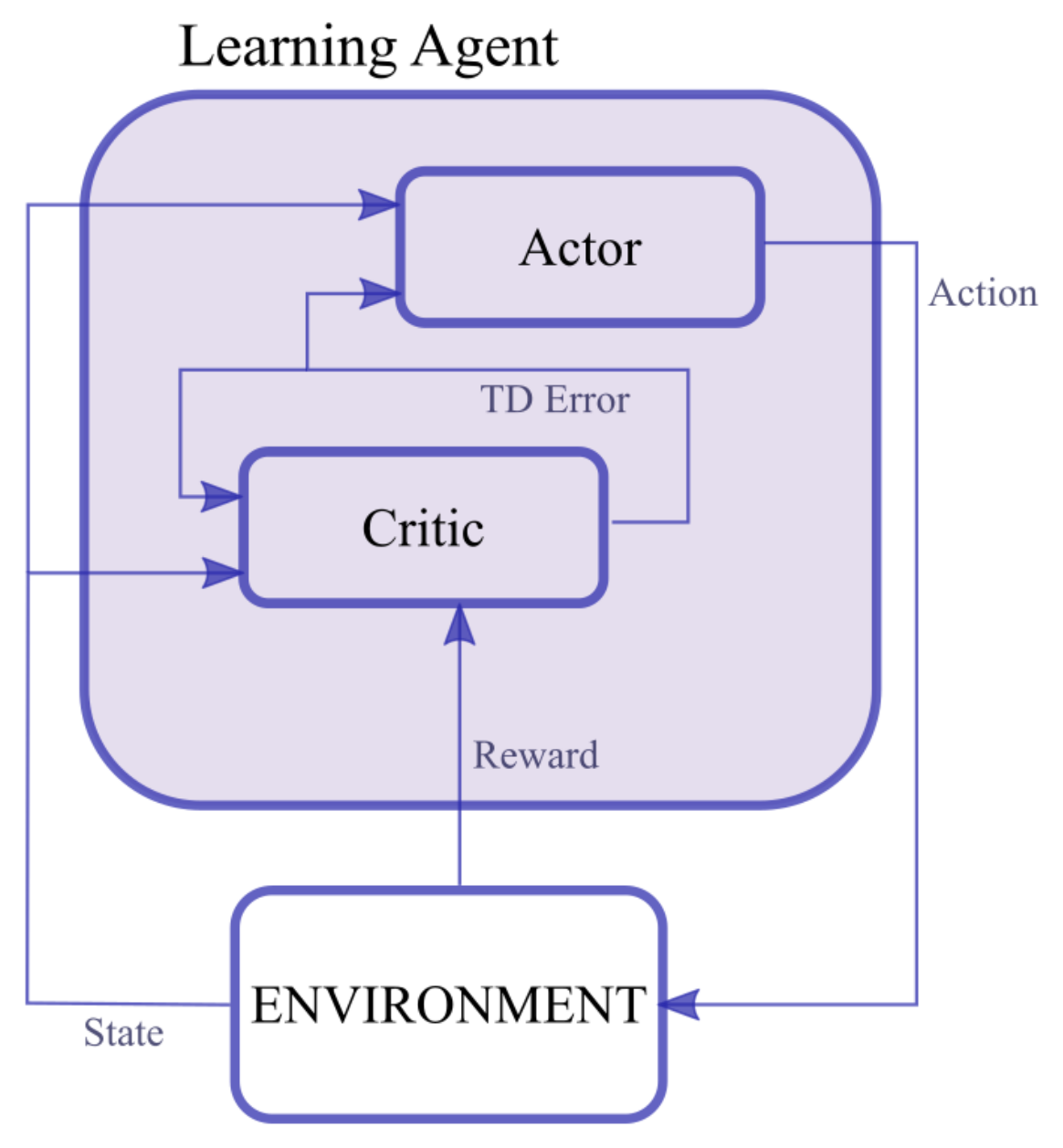
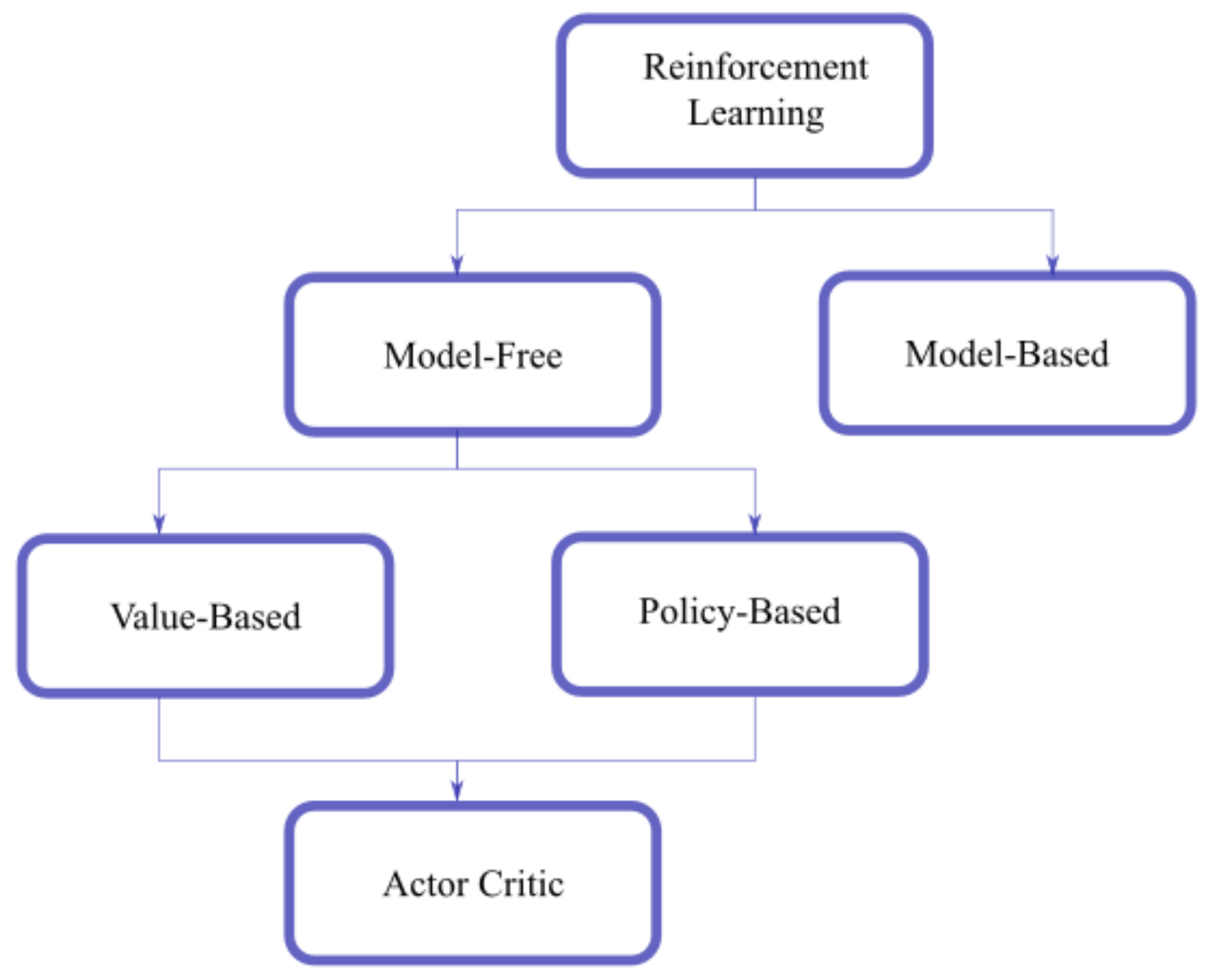
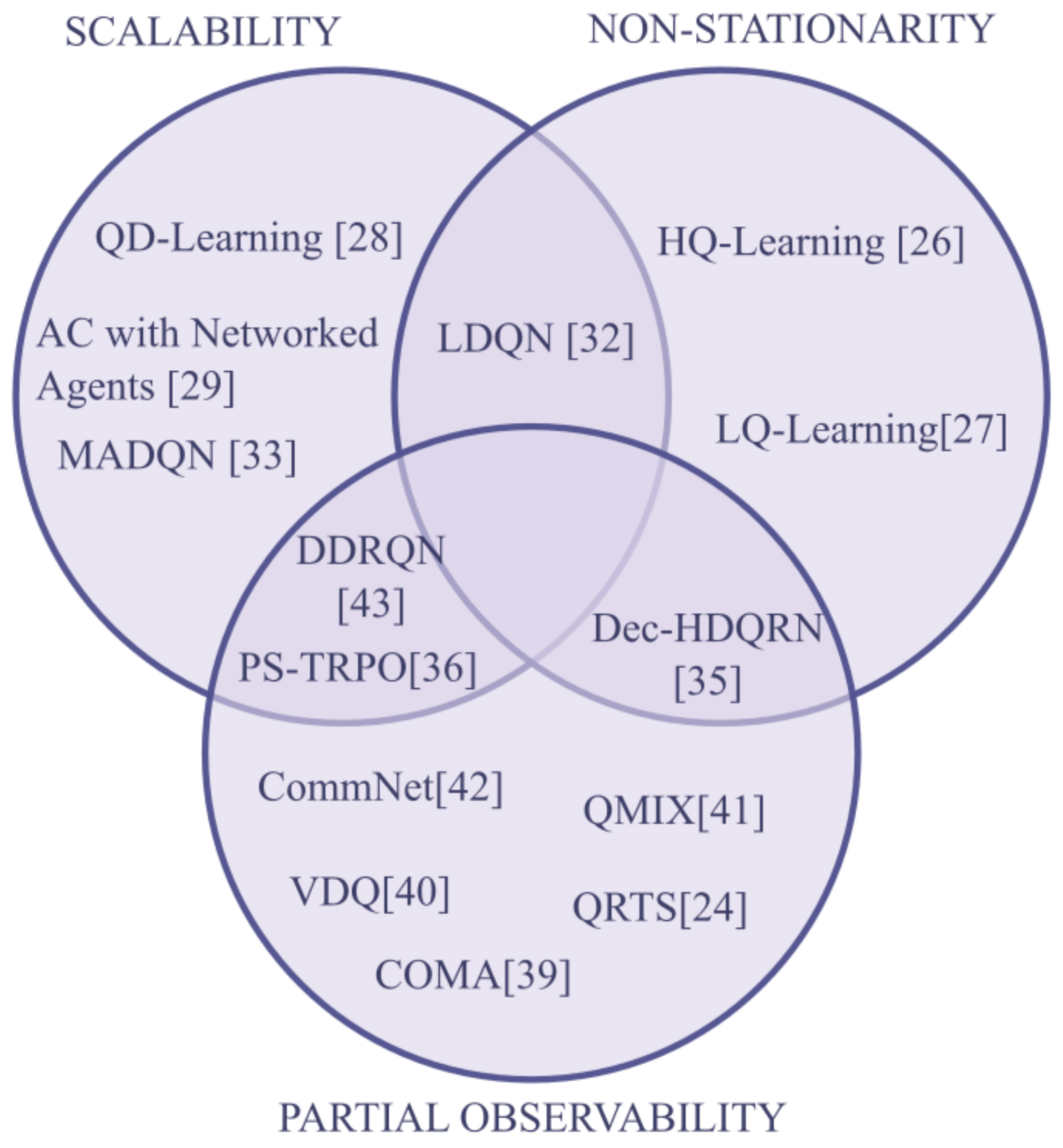
Table 1.
Summary of MARL algorithms.
| Algorithm | Type of Agent | Learning Structure | Features | Scientific Spreading |
|---|---|---|---|---|
| Hysteretic Q-Learning [26] | Value based | Independent learners | Uses a different learning rate for increasing and decreasing Q-values. No need for communication between agents | 1100 |
| Lenient Q-Learning [27] | Value based | Independent learners | Accumulates rewards for a state–action-pair and then update it using the maximum reward | 333 |
| QD-learning [28] | Value based | Networked agents | Receives the Q-values from agents in the proximity with the objective of minimizing the difference and reaching consensus | 104 |
| Actor–Critic with Networked Agents [29] | Actor–critic | Networked agents | Both the policy of the actor and the Q-estimates of the critic are parameterized. The agents share the parameters of their critic to reach consensus | 3050 |
| Lenient deep Q-network [32] | Value based | Independent agents | Stores a temperature variable in the experience replay to decide the amount of leniency to apply to the updates | 97 |
| Multi-Agent Deep Q-Network [33] | Value based | Independent agents | Use of importance sampling and low-dimensional fingerprints to disambiguate samples in the experience replay | 3380 |
| Dec-HDQRN [35] | Value based | Independent agents | Integrates the recursive neural network to estimate the non observed state and hysteretic Q-learning to address non stationarity. Possibility to use transfer learning to adapt to multi task applications | 49 |
| PS-TRPO [36] | Policy optimization | Centralized training | Shares parameters between agents during training. The policy parameters are bounded to change in a trust region. Can scale progressively to more agents using curriculum learning | 23 |
| COMA [39] | Actor–critic | Centralized training | A centralized critic is used only during the training phase. Can differentiate rewards between agents using a conterfactual baseline | 4750 |
| VDN [40] and QMIX [41] | Value based | Networked agents | The Q-table of the joint action can be factorized as a sum or a combination of independent Q-Tables | 847 |
| CommNet [42] | Policy optimization | Networked agents | The agents communicate for a number of rounds before selecting their action. The communication protocol is learned concurrently with the optimal policy | 319 |
| DDRQN [43] | Value based | Networked agents | Uses a deep recursive network architecture in a partial observable setting with the use of parameter sharing to speed-up the learning process | 3510 |
| Q-RTS [24] | Value based | Centralized training | Agents create a global knowledge Q-matrix combining their most valuable experiences and make updates on a linear combination of the matrix and their local Q-table. | 108 |
Table 2.
Applications of MARL algorithms divided by field of use.
| Sector | Applications |
|---|---|
| UAVs | Drone field coverage [47] Target assignment and path planning [48] LoS Networks [50] Packet routing relaying [52] Recharging towers [53] |
| Image processing | Joint active objective search [54] |
| Energy sharing and scheduling | Zero-energy community [55] Residential microgrid with V2G exchange [56] Industry production control [58] Lithium battery lifetime optimization [64] |
| Automotive | Safe driving [59] Fleet control for ride sharing platform [61] Intersection traffic light control [62] |
| Social Science | Common Pool Resource Approximation [66] Sequential Social Dilemmas [67] |
| Networking | Base-station parameter approximation [68] |
Publisher’s Note: MDPI stays neutral with regard to jurisdictional claims in published maps and institutional affiliations. |
© 2021 by the authors. Licensee MDPI, Basel, Switzerland. This article is an open access article distributed under the terms and conditions of the Creative Commons Attribution (CC BY) license (https://creativecommons.org/licenses/by/4.0/).
Share and Cite
MDPI and ACS Style
Canese, L.; Cardarilli, G.C.; Di Nunzio, L.; Fazzolari, R.; Giardino, D.; Re, M.; Spanò, S. Multi-Agent Reinforcement Learning: A Review of Challenges and Applications. Appl. Sci. 2021, 11, 4948. https://doi.org/10.3390/app11114948
AMA Style
Canese L, Cardarilli GC, Di Nunzio L, Fazzolari R, Giardino D, Re M, Spanò S. Multi-Agent Reinforcement Learning: A Review of Challenges and Applications. Applied Sciences. 2021; 11(11):4948. https://doi.org/10.3390/app11114948
Chicago/Turabian StyleCanese, Lorenzo, Gian Carlo Cardarilli, Luca Di Nunzio, Rocco Fazzolari, Daniele Giardino, Marco Re, and Sergio Spanò. 2021. "Multi-Agent Reinforcement Learning: A Review of Challenges and Applications" Applied Sciences 11, no. 11: 4948. https://doi.org/10.3390/app11114948
Note that from the first issue of 2016, this journal uses article numbers instead of page numbers. See further details here.