Article

Analysis of Fluid Velocity inside an Agricultural Sprayer Using Generalized Linear Mixed Models

by
Ángel Javier Aguirre
1,*,
Guillermo E. Guevara-Viera
2,
Carlos S. Torres-Inga
3,
Raúl V. Guevara-Viera
2,
Antonio Boné
4,
Mariano Vidal
4 and
Francisco Javier García-Ramos
4
1
CPIFP Montearagón, 22071 Huesca, Spain
2
Faculty of Agricultural and Livestock Sciences, University of Cuenca, 010205 Cuenca, Ecuador
3
Department of Mathematics and Statistics, University of New Mexico, Albuquerque, NM 87106, USA
4
Higher Polytechnic School, University of Zaragoza, 22071 Huesca, Spain
*
Author to whom correspondence should be addressed.
Appl. Sci. 2020, 10(15), 5029; https://doi.org/10.3390/app10155029
Submission received: 9 July 2020 / Revised: 15 July 2020 / Accepted: 20 July 2020 / Published: 22 July 2020
(This article belongs to the Section Mechanical Engineering)

Abstract

:
The fluid velocity inside the tank of agricultural sprayers is an indicator of the quality of the mixture. This study aims to formulate the best generalized linear mixed model to infer the fluid velocity inside a tank under specific operational parameters of the agitation system, such as liquid level, circuit pressures, and number of active nozzles. A complex model was developed that included operational parameters as fixed effects (FE) and the section of the tank as the random effect. The goodness of fit of the model was evaluated by considering the lowest values of Akaike’s information criteria and Bayesian information criterion, and by estimating the residual variance. The gamma distribution and log-link function enhanced the goodness of fit of the best model. The Toeplitz structure was chosen as the structure of the covariance matrix. SPSS and SAS software were used to compute the model. The analysis showed that the greatest influence on the fluid velocity was exerted by the liquid level in the tank, followed by the circuit pressure and, finally, the number of active nozzles. The development presented here could serve as a guide for formulating models to evaluate the efficiency of the agitation system of agricultural sprayers.

1. Introduction

The velocity of the fluid inside an agricultural sprayer, necessary for the homogeneous mixing of the active matter, is determined by the internal agitation system, which is hydraulic in most cases. It differs according to (a) certain working parameters such as circuit pressure, number of active nozzles, and liquid level in the tank; and (b) the geometry of the tank height, width, section type, presence of barriers and irregularities inside the tank, and the location of the nozzles.
The combination of these two sets of parameters makes it difficult for the observed fluid velocity data to fit a normal distribution. This requires the use of non-parametric methods when evaluating possible velocity variations based on working and geometry parameters [1]. This analytical approach helps reveal the effect of the parameters separately, masking the possible interactions between them, as well as the weight that each one exerts on the velocity variations.
Fluid velocities inside spray tanks can be correlated with the efficacy of the agitation. Xiongkui et al. [2] concluded that the efficacy of agitation was improved by increases in both flow rate and working pressure; similar conclusions were obtained by [3]. In turn, it can be concluded that an increase in fluid velocity will produce an improvement in the efficacy of the agitation system [4]. Different studies have investigated fluid velocities inside spray tanks using Computational Fluid Dynamics (CFD) [5]. The use of this type of model is very useful, but it has the drawback of requiring long calculation times and the need for very precise data on the geometry of the interior of the tank and the location and characteristics of the components of the agitation system [6]. In this sense, Generalized Linear Mixed Models (GLMM) are an alternative to the CFD.
GLMM extend the set of generalized linear models by adding random effects to the linear estimator [7], allowing the modelling of correlated observations. In addition to generalized linear models [8], the GLMM can be formulated using a three-part sequence [9], on the basis of its general formulation [10,11] (Equation (1)).
y = X β + Z u + ε
where y = n × 1 observed data in a column vector; X = n × p matrix of the p predictor variables (all levels of fixed effects); β = p × 1 column vector of the fixed-effects regression coefficients; Z = n × q design matrix for the q random effects; u = q × 1 vector of the random effects; ε = n × 1 unobserved error vector.

1.1. Theoretical Sequencing of the Model

The conditional distribution of each yij, given a vector q × 1 of random effects ui, belongs to the exponential family of distributions (positive or negative binomial, Poisson, normal, and gamma, among others). The variance is given by (yij|ui) = ϕυ(E(yij|ui)), where, υ(·) is a known function for the variance, a function of the conditional mean E(yij|ui), and ϕ is a scalar parameter that may be known or needs to be estimated. It should be noted that, given the random effects ui, it is assumed that values of yij are independent of each other, which assumes conditional independence [12].
The conditional mean of yij, which is dependent on the fixed effects (FE) β and random effects (RE) ui, is linked to the linear predictor ηij, through the application of a known linkage function, g(·), which is monotonous and differentiable [13], as follows (Equation (2)):
g{E(yij|ui; xij; zij)} = ηij = xijTβ + zijTui,
where, xij and zij are two vectors of covariates p × 1 and 1 × q dimensional, respectively.
Although any function can be chosen for g(·), each distribution belonging to the exponential family has a special linking function called the canonical linking function. The known linkage function g(·) is given by (Equation (3)):
g{E(yij)} = θi,
where, θi is the canonical location parameter.
Generally, any multivariate distribution can be supported for ui. In practice, it is common to assume that the ui has a multivariate normal distribution [14], with zero mean and variance-covariance matrix G, sized q × q [15], where G is some function of θ. Additionally, the RE ui are assumed to be independent of covariates xi, if any.
The adjustment of the model requires the maximization of the marginal likelihood, which is obtained by integrating the RE. The form of distribution of RE has a notable influence on the unbiased inference of the maximum likelihood estimators (MLE) of FE [14]. Software packages offer several answers to solve this [16].
SPSS and SAS, by default, use iterative linear methods that maximize the penalized quasi-likelihood residual (PQL [17,18,19]; RSPL method in SAS), whose main criticism is that the inference of the plausibility that it may be inappropriate, as it generates a bias for large variances or small means. Existing methods to approximate the likelihood to estimate GLMM parameters include, marginal quasi-likelihood methods (MQL) [20], Laplace approximations [21], Gauss-Hermite quadrature (GHQ) [22], and Markov chain Monte Carlo (MCMC) algorithms [23]. Adaptive quadrature (GHQ) or Laplace approximations are the preferred methods for categorical response variables [15,22,24]. Residual methods account for the FE in the construction of the objective function, which reduces the bias in covariance parameter estimates. Estimation methods involving the Taylor series create pseudo-data for each optimization, which are transformed to have a zero mean in a residual method. While the covariance parameter estimates in a residual method are the maximum likelihood estimates for the transformed problem, the fixed-effects estimates are (estimated) the generalized least squares estimates. In a likelihood method that is not residual based, both the covariance parameters and the fixed-effects estimates are maximum likelihood estimates, but the former are known to have greater bias. In certain problems, residual likelihood estimates of covariance parameters are unbiased.
The degrees of freedom (df) for RE, required for Wald tests or F tests or Akaike’s information criteria (AICc), must be between 1 and N-1 (where N is the number of RE levels). Software packages vary enormously in their approach to computing df. The simplest approach uses the minimum number of df contributed by RE that affect the term being tested (residual method) [25]. The Satterthwaite and Kenward-Roger (KR) approximations [25,26] use more complicated rules to approximate the df and adjust standard errors.
The overview of the model implies that the variance matrix of the target variable has the following form: V = ZGZ’ + R. Knowing that ε is the vector of unobserved errors, the variance takes the form of (Equation (4)):
V a r [ u ε ] = [ G 0 0 R ]
The R matrix is by default the scaled identity matrix, R = σ2I, where I is the n × n identity matrix, and G is a diagonal matrix containing variance components [27]. The usual estimate of the variance-covariance matrix of the mean model parameters depends on the specified variance-covariance model for the data. The consideration of a wide class of variance-covariance models helps ensure that this specification is logical [28].

1.2. Objective

This study aims to explore, describe, and adjust a generalized linear mixed model, appropriate for the analysis of the influence that each variable (geometric and agitation system regulation) exerts on the internal velocity of the fluid. Considering that these models allow the dependent variable to not have a normal distribution [29], there are correlated observations and a linear relationship with the independent variables and covariates through a given linkage function.

2. Material and Methods

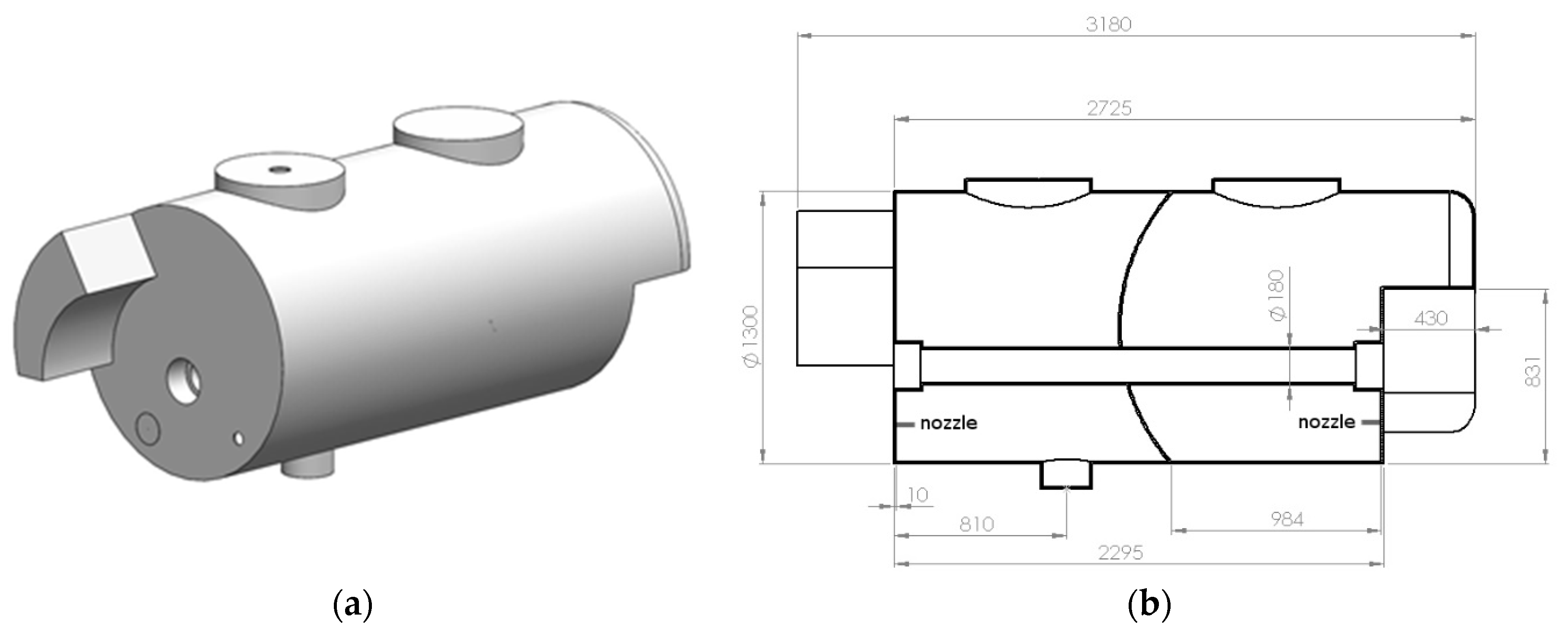
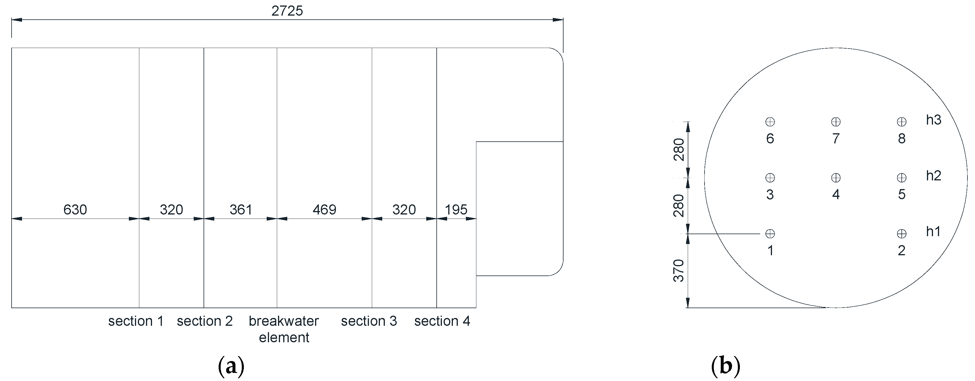
2.1. Source of the Data

For this study, the data from the trial conducted by [4] with a hydropneumatic sprayer tank (Figure 1) was used, in which the fluid velocity (cm/s; FV) was measured using a 3-D microacoustic Doppler velocimeter, at 32 points, distributed in several positions inside the tank (Figure 2; height-H; side-S; and section-SC), and at varying pressure of the agitation system (8, 10, 12 bar; P), number of active nozzles (2, 4; NN), and liquid level in the tank (1000, 2000, 3000 L; LT). General terminology notation is specified in Table 1.

2.2. Software Used

The SPSS package (IBM Corp. Released 2017. IBM SPSS Statistics for Windows, Version 25.0. Armonk, NY: IBM Corp.) and PROC GLIMMIX of SAS/STAT, version 9.4 of the SAS System for Windows (SAS Institute Inc. 2018), whose scripts are shown in Appendix A, were used.

2.3. Useful Sequencing of the Best Model

In this study, for the formulation and selection of the best model in terms of the number and nature of the fixed and random effects (Table 2, Table 3 and Table 4), a canonical link function was assumed under the premise of a normal distribution of the errors of the model and the target variable, fluid velocity (FV). The Kolmogorov–Smirnov (K–S) test was used to evaluated conformance with the normal distribution (theoretical curve shown in Figure 3). Once the best model was selected and the FV showed positive scale values that deviated towards larger positive values, it was tested until the combination “distribution form-linking function”, providing a better fit, was obtained.
With respect to the variance-covariance matrix, the basic rationale was that “parsimony means power”, that is, to obtain the most efficient inferences about the mean model, one selects the most parsimonious covariance structure possible, that continues to reasonably fit the data. It is, thus, recommended, in each case, to test both the formats with the least number of parameters and heterogeneous structures [30].
Table 5 shows estimates of mean and variance of the Pearson’s residues according to the different covariance matrix structures tested. A linear regression was performed between the predicted and observed values (Table 6), assessing their significance through an analysis of variance of the regression model, the constant, and the slope. The results obtained with the best model, through SPSS and SAS, through three iterations, using the information criteria and the estimates of the residual variances (Table 7); using estimated averages for the different levels of FE and theirs p-values (Table 8 and Figure 4); and through the adjustment coefficients of a regression between observed and predicted values, were compared (Table 9).
The relationship between the observed and predicted values estimated using the best model is represented in Figure 5, through the linear regression that relates them. Starting from this, 95% predictor intervals are shown, whose calculation responds to what is explained in (Equation (5)) [31]. The points excluded from the prediction interval, the section they belonged to, and the dispersion statistic that characterized them were identified.
y i y ^ i ± t α / 2 , n 2 σ ^ 2 [ 1 + 1 n + ( x i x ¯ ) 2 S x x ]

3. Results and Discussion

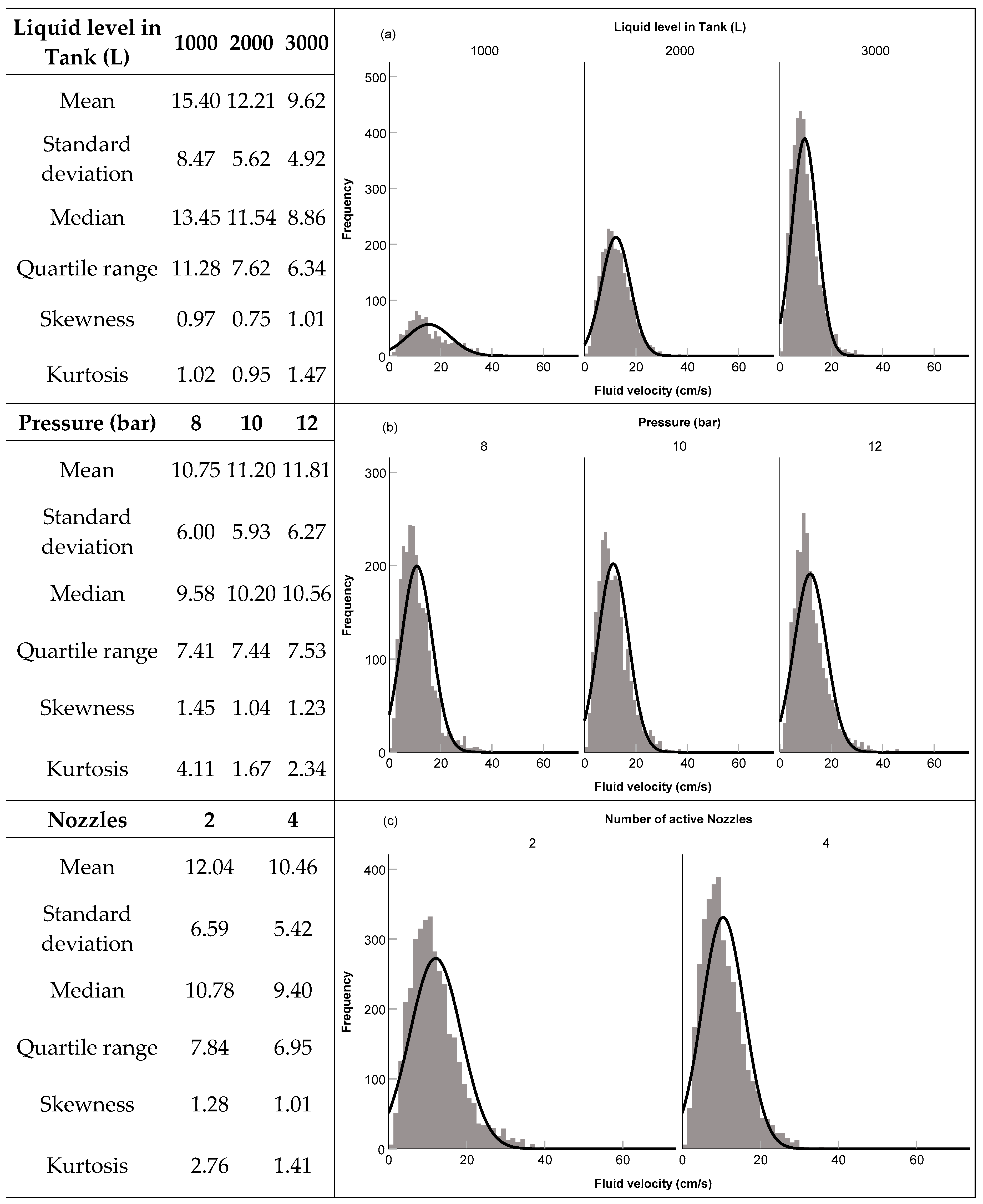
3.1. Distribution Analysis of the Targeted Variable: Fluid Velocity

The analysis of the fluid velocity (cm/s) variable as a whole (n = 7200) revealed an average value of 11.25 ± 6.08 cm/s, within a range of values from 0.69 cm/s to 61.73 cm/s, highlighting a mismatch with the normal distribution (K−S = 0.08; p < 0.001). The representation of the data based on the operational parameters of interest: LT, NN, and P, showed various extremes and outliers in the right tail of the distribution, with Skewness = 1.24, and Kurtosis = 2.68 (Figure 3). It is known that, to develop models that describe what is observed in reality, the variable should not be transformed, nor should extremes and outliers be treated and/or eliminated [32].

3.2. Model Comparison

Models without interactions between FE and with an increasing level of complexity were developed, whose fit was compared with (a) the AICc corrected [33,34], despite a high number of observations in relation to the number of parameters in the model (K), such that n/K > 40, and (b) the Schwarz’s Bayesian criterion (BIC) [34,35], which modifies the model parameter scores with respect to the AICc (Table 2). This obviates the need to establish a level of significance in accepting or rejecting effects, similar to the stepwise method [36].
As can be seen in Table 2, the best model showed a lower value of the AICc and BIC information criteria coefficients, and also the highest relative Akaike weight (wi; Table 3). The model that best represented the reality measured by the data, was number 11, which included the operational parameters of liquid level in the tank, number of active nozzles, and pressure, with FE and the section of the geometric shape of the tank as a RE. Models 12 and 13, respectively, followed this with a decreasing plausibility in terms of adjustment to the observed data.
Model 11, together with the Models 12 and 13, were those that estimated the lowest residual variance among the other models (Table 4).
Models which excluded SC, in the fixed and the random effects (Models 1 to 10 and 14), showed the lowest relative weights (wi) in the aggregate, and the highest estimates of residual variance. The smallest values of residual variance, corresponding to the models that best fit the description of the observations [37] highlight the importance of SC, as a descriptor of the sprayer tank geometry, when assessing the velocity of the fluid inside, and the need for their inclusion as RE and not as FE.
The practical use of such sprayers causes them to gain importance in the interactions between the factors [38]. Nevertheless, the introduction of double interactions: LT×P, LT×NN, and P×NN, and the three-way interaction: LT×P×NN, among the FE, barely improves the fit by 0.41% (∆AICc = −179.75). It must be highlighted here that, the interaction double, LT×P, displayed greatest influence (absorbed more variability) on the fluid velocity inside the tank. Since the formulation of an efficient model was tested here, the inclusion of the double and triple interactions were dismissed, even as RE [29] (the G matrix did not converge), to simplify the interpretation of the results.
In this type of GLMM models, the normal parametric distribution for RE has been assumed [39]. This is mainly for conventional reasons [40], understanding that, despite having chosen four cross-sections for the location of the control points within the sprayer’s tank, the cut-off point for the choice of the section could take any value from one end to the other. It should be remembered that it is not highly recommended that random effects have many levels so that the Z matrix can converge [27].
No further information was provided on the form of the joint distribution of the RE (SC, H, S), and, thus, the normal distribution assumption, for these RE as a whole, was not evaluated directly in the Models 12, 13, and 14 [41]. The choice of a RE only partly outweighs the natural concern about the incorrect specification of RE in GLMM models [42], and its possible impact on the FE inferences [43].
No evidence was found of the use of GLMM in the analysis of the operation of the agitation system of agricultural sprayers. Until now, studies carried out in this regard have focused on the use of linear models such as ANOVA [4] or numerical modeling using CFD [1,6]. Therefore, the GLMM application methodology proposed in this research can be extended to different tank geometries (cylindrical, asymmetric, cubic, etc.) and to different designs of the agitation system (number of nozzles, location of nozzles, etc.).

3.3. Best Model Description

The data was structured from control points, as observation units that were independent of each other. The measurements were carried out according to different levels of the FE, such as liquid level in the tank, pressure, and the number of active nozzles, in four sections and at three heights and distances from the perimeter (sides).
The target variable (dependent) is the fluid velocity inside the tank. As previously warned, considering the form of the distribution of the target variable and the outcome of the various tests carried out, the combination that best matched what was observed was a Gamma-type distribution [31] with a logarithmic link function (f(x) = log(x)).
The values of the information criteria after the assessment of the different forms of the variance-covariance matrix (Table 5) show that, in the case of the AICc, the structures that best fit the model are the First-order autoregressive moving-average, followed by the Toeplitz, while with the BIC, the best fit model was the identity model followed by the first-order autoregressive, and then the first-order autoregressive moving-average model, which corresponded to their respective relative weights (wi AICc or BIC). Among these, the model that recorded a minor statistical significance for σ ^ 2 SC was the Compound-symmetry covariance structure, being the one that most closely related the observations to the assumption of independence [19,44].
Despite having a large number of observations, and only one RE, it was difficult to choose the most appropriate covariance structure based only on the information criteria shown in Table 5 [45]. The degree of adjustment of the model’s predictions to the observed data was, thus, analyzed according to the different covariance structures (Table 6) [27,28].
The accordance between the observed and predicted values of the model with regard to the determination coefficient, based on the structure of the covariance matrix (Table 6), revealed that the best fit corresponded to Unstructured and Toeplitz. The smallest standard error in the estimation was provided by First-order autoregressive moving-average, followed by the Identity. As for the estimation of the variance of Pearson’s residues, the values closest to unity came from Unstructured, followed by the Toeplitz. Pearson’s average residue estimate was very close to zero for all structures.
Through the AICc and BIC information criteria (Table 5), and with the coefficients of fit between what was observed and what was predicted by the model (Table 6), it seems that the Toeplitz covariance structure could be the most appropriate for the case under consideration (Equation (6)), obtaining the following p-values: p( σ 2 ) = 0.001; p( σ 1 ) = 0.308; p( σ 2 ) = 0.367; and p( σ 3 ) = 0.001. This shows that the variability of the fluid velocity within each level of SC was significant, as was the difference in the observed variability between the first and last sections of the tank.
T o e p l i t z   c o v a r i a n c e   s t r u c t u r e = [ σ 2 σ 1 σ 2 σ 3 σ 2 σ 1 σ 2 σ 2 σ 1 σ 2 ] = [ 0.060 0.011 0.015 0.036 0.060 0.011 0.015 0.060 0.011 0.060 ]
The number of samples in this test was high, and only one RE was included, which made it difficult to bias the iterative linear methods that maximize the PQL. The Laplace and Gauss-Hermite quadrature approaches were tested, resulting in higher (worse) values in the AICc and BIC information criteria (41,652.69). The MQL method was also tested, obtaining lower (better) values in the information criteria with respect to the PQL. A lower adjustment, however, between what was inferred and what was observed, as well as a clear bias due to excess in the estimation of the FE was observed.
The KR [46] and Satterthwaite [47] approaches for the calculation of degrees of freedom did not improve the reporting criteria and the estimation of residual variance, compared to the Between-Within, Containment, and Residual methods. Thus, without complicated covariance structures, when the sample size is moderate to large, and the design is reasonably balanced, similar to the case considered here, the Between-Within method offered greater accuracy and compatibility with robust fixed-effects estimators [48]. As the approximate variance matrix of the fixed-effects estimates depends on the estimation method, assuming the least square mean is estimable, PROC GLIMMIX constructs an approximate t-test to test the null hypothesis that the associated population size equals zero. By default, the denominator for degrees of freedom for this test was the same as that of the effect in the type III tests of FE, although the Between-Within method divided the residual degrees of freedom into between-subject and within-subject portions so that PROC GLIMMIX determined changes in a FE within any subject. If so, it assigned the within-subject degrees of freedom to the effect, and assigned the between-subject degrees of freedom to the effect, if otherwise [49]. As multiple effects within the subject (measurement point) were related to the classification variables (LT, P, and NN), the degrees of freedom within the subject were divided into components that correspond to the subject of the interactions by the effect. Therefore, Tukey’s test was conducted with the row adjustment, and multiple comparisons of the probability and confidence intervals were obtained for the differences between the least quadratic means of the FE levels [50].
The tests of effects and fixed coefficients were carried out with SPSS, and robust estimation was applied, in view of the extreme and atypical data whose effect could violate the homoscedasticity premise of the model [7,12]. In SAS, various estimators (known as sandwich or empirical) reduce to the heteroscedasticity consistent covariance matrix estimators (HCMM) [51]. Based on simulations in regression models, some authors strongly recommend the one known as HC3 estimator to accommodate non-normal data and correlated observations [52,53]. This approximation was motivated as a jack-knife estimator, based on the “leave-one-out” estimates of β ^ [54].

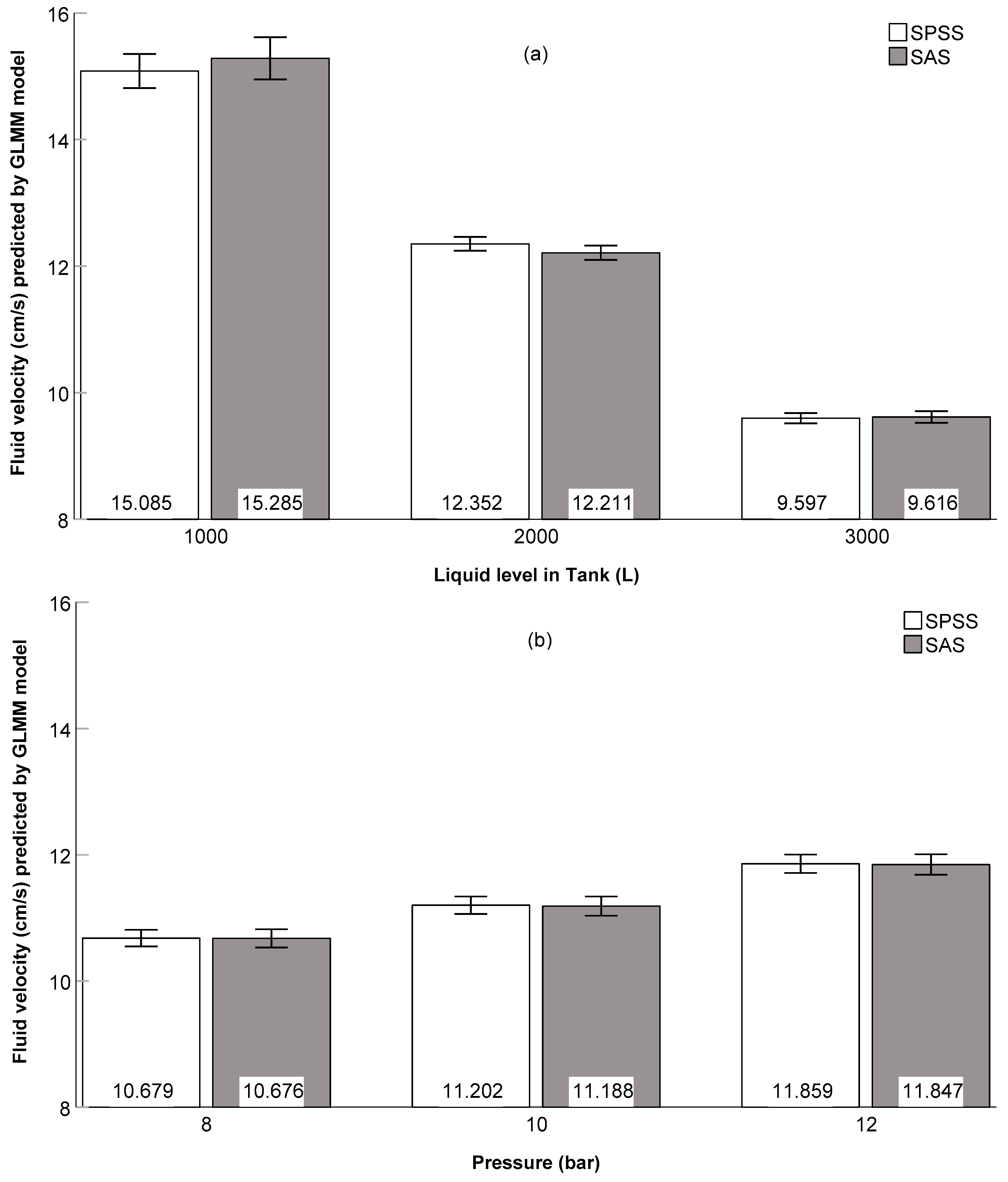
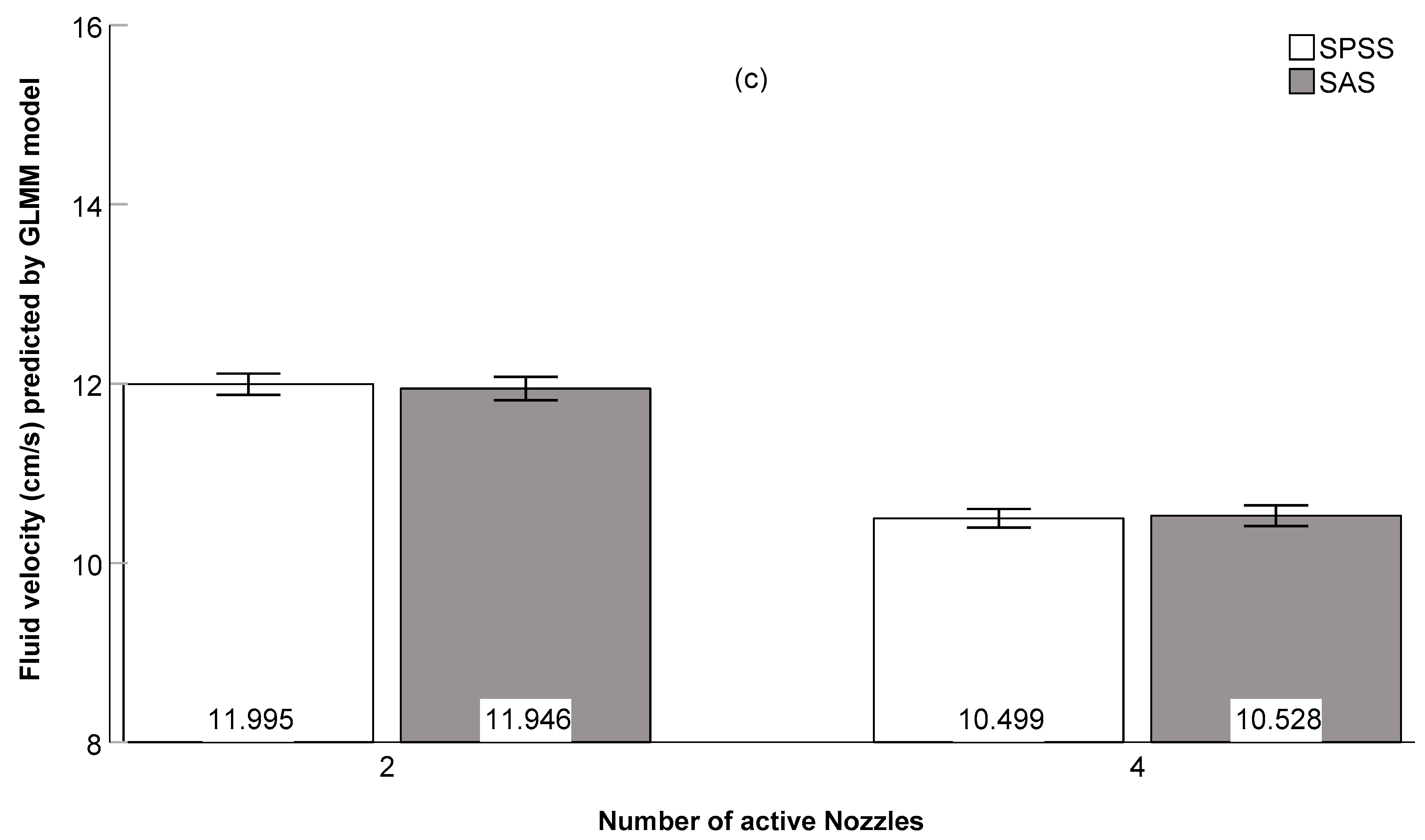
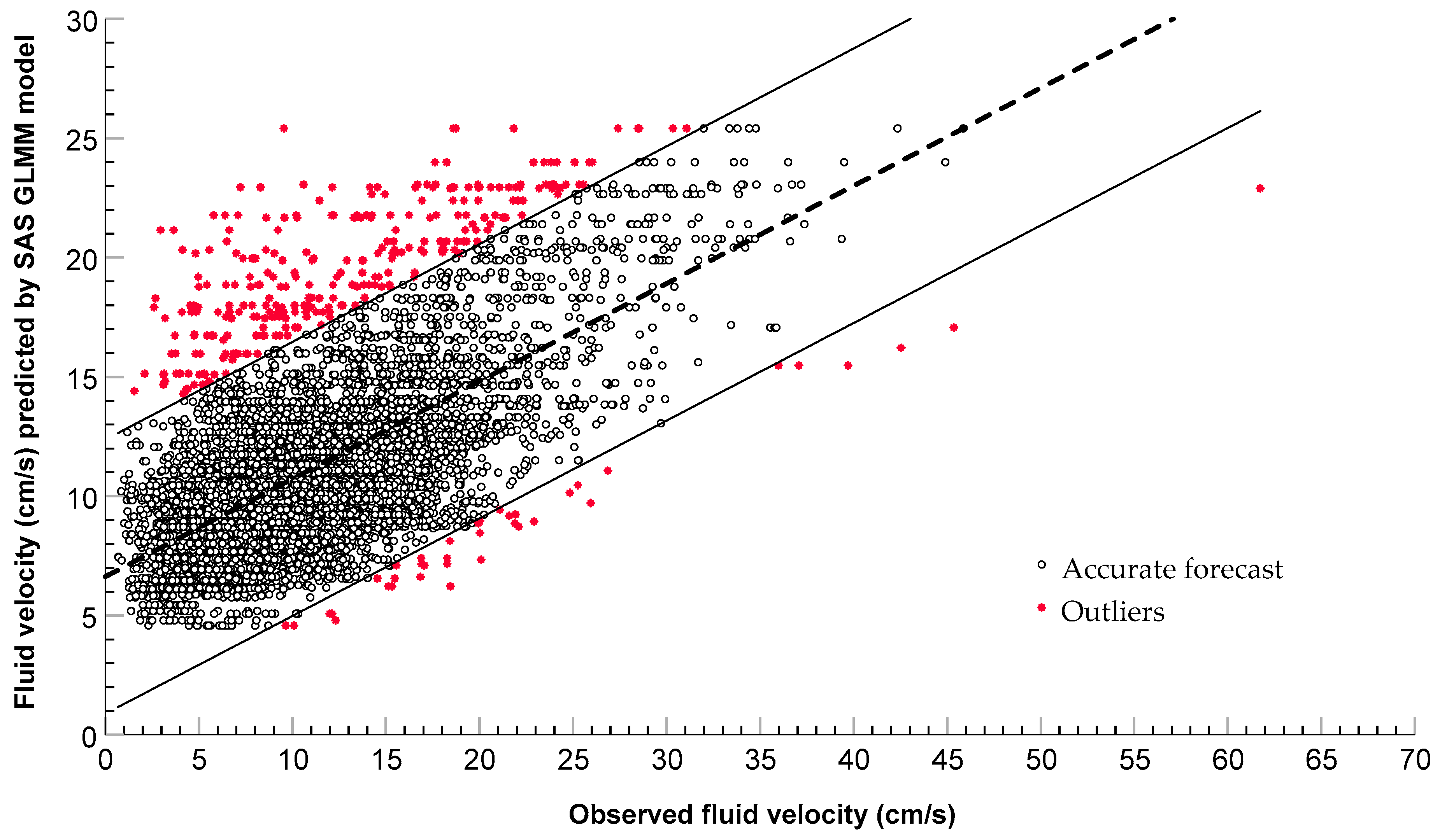
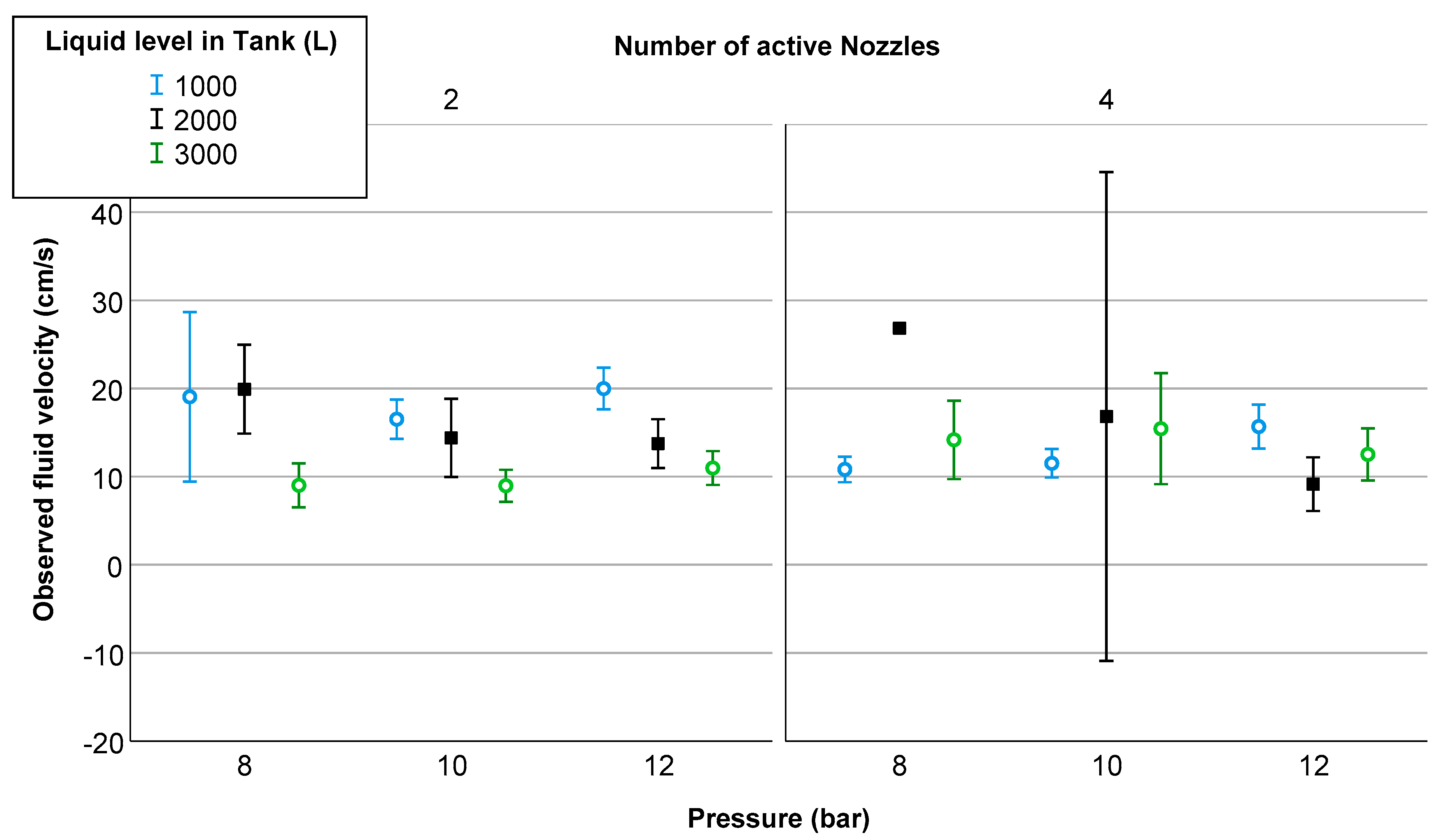
3.4. Comparison of IBM SPSS and SAS Model Results

The estimate of the residual variance and the estimated variance of Pearson’s residues, predicted by the model computed through SAS, offered better values than the one computed through SPSS (Table 7). Additionally, SAS showed the ratio of the generalized chi-square with its degrees of freedom, which is a measure of the variability of the observation on the mean model.
The distribution of Pearson’s residues on the predicted values did not fit a normal distribution in either case. However, the probability of the result of the model computed with SAS showed a lower significance (K–S = 0.029; p = 2.79 × 10⁻¹⁵) than the one computed with SPSS (K–S = 0.034; p = 4.61 × 10⁻²¹).
As shown in Table 8, with the exception of the number of active nozzles in the SPSS model, all three FE had a significant effect on the internal fluid velocity. Both software showed that the level of liquid in the tank (TL) had the greatest influence on the fluid velocity, followed by the agitation system pressure (P), and finally, the number of open nozzles (NN). Considering the SPSS model, the most different FE was the number of open nozzles, as it seemed to have the least influence, with respect to the other two (<F). Considering the SAS model, the agitation system pressure and the number of open nozzles had a significant effect, and which was more similar to each other and much less than that of the liquid level in the tank.
Results obtained with both software agreed that fluid velocity was significantly lower as the liquid level inside the tank increased. While no differences were observed at 8 or 10 bar, the fluid velocity increased significantly when the pressure reached 12 bar. However, the results differed in the effect of the number of active nozzles. While the SPSS model did not observe differences between the presence of 2 and 4 open nozzles, the SAS model observed and separated them, highlighting that the velocity was significantly lower with four open nozzles, potentially due to their geometric location in the tank as they were facing each other (Figure 1).
Thus, when the four nozzles operated, the liquid flowed facing 2 to 2 and produced a braking effect. In this case, the four nozzles were arranged on the same work plane and aligned with two sets of nozzles facing each other, with each pair located at the ends of the tank. In contrast, when two nozzles were used, they were located in the same plane but misaligned with each other, and thus did not directly face the fluid flows. There was, however, a gap in the flow lines of approximately 700 mm. This is consistent with the significance of the σ3 covariance, between the first and last section, observed in the Toeplitz variance-covariance matrix (Equation (6)). Generally, the least square means obtained with SAS were slightly higher than those obtained with SPSS, with the exception of the cases of 2000 L and 3000 L of liquid in the tank.
The predictions on the fluid velocity of the best model revealed significant differences between all the levels of FE (Figure 4). It is noteworthy that these were slightly lower than those observed during the test (Table 8), with the differences between what was predicted by the SPSS and SAS models, and the differences in the analysis of the observations made by both software being in a certain proportion.
Without the pretension of establishing a correct linear regression, as several of its premises are not fulfilled, if this method was used to find the output that adjusts its predictions with the measurements in the laboratory better, it was observed that the best model, computed with SAS, revealed a better adjustment in the coefficient of determination (R2; almost 8%), a higher correlation and, the residues, having less skewness and kurtosis, than that computed using SPSS (Table 9).
Therefore, the best model was the one computed with SAS, considering the parameters that have been discussed throughout the study. However, the predicted values reproduce the highest values in the positive direction of the target variable, fluid velocity (FV), overestimating some predictions from 2 cm/s to 32 cm/s, but reducing the maximum predicted velocity by at least 15 to 17 cm/s (Figure 5). The best fit occurred when the liquid level in the tank was 1000 L (R2ad = 0.467), at a pressure of 8 bar, with two active nozzles (R2ad = 0.661). The model setting for the variable pressure was better for a pressure of 8 (R2ad = 0.453) and 12 bars (R2ad = 0.410), as opposed to 10 bars (R2ad = 0.392). Finally, the model was always better adjusted with two active nozzles (R2ad = 0.456) than with four (R2ad = 0.352). The model’s worst adjusted combination of variables occurred with LT = 2000 L, P = 12 bar, and NN = 2 (R2ad = 0.146).
The values excluded from the prediction limits in Figure 5 are those whose residue exceeding twice the width of the 95% prediction interval (e ≥ 5.85; Equation (5)). Sixty-nine percent of these were measured in Section 2, with σ2FV,SC2 all data = 49.27 (n = 1800) versus σ2FV,SC2 excluded data = 52.74 (n = 255), which was the closest to the breakwater element; while 21% were measured in Section 1, with σ2FV,SC1 all data = 39.10 (n = 1800) versus σ2FV,SC1 excluded data = 42.31 (n = 80). This shows that the excluded values in each section not only contain the variability of the whole section but also exceed it. In this regard, the following combination of FE levels are highlighted: LT = 2000 L, P = 10 bar, and NN = 4, with σ2FV excluded data = 124.67 (Figure A1 in Appendix B).

4. Conclusions

The best model tested included the liquid level in the tank, circuit pressure, and number of active nozzles as FE, and only the section of the tank as RE; height, and side of the control points, being irrelevant. The inclusion of double and triple interactions among the FE hardly improved the fit of the best model and did not favor the interpretation of the results.
After the obligatory singular evaluation in the choice of the covariance structure, particularly for the fixed and random effects of this study, the Toeplitz covariance matrix structure showed the best values in terms of information criteria and adjustment between predicted and observed data as a whole. However, agreeing with prior studies, this structure did not show a conclusive advantage over other structures, so its choice could be discussed.
Using SPSS, the Satterthwaite approximation could be performed for the calculation of the degrees of freedom while using robust estimation methods for the tests of FE and coefficients. With SAS, however, the Between-Within method and the HC3 estimator were used. The best model in terms of reporting criteria was obtained using SAS.
Through this generalized linear mixed model, it has been possible to evaluate fixed and random effects together so that the FE that most influenced the fluid velocity could be identified as the liquid level in the tank, followed by circuit pressure, and finally, the number of active nozzles. The results obtained for the variable liquid levels in the tank and circuit pressure showed similar significant differences considering the best model calculated with both software. However, they differed with regard to the significance of the effect of the active nozzle. While the SAS calculation observed a significant effect, the SPSS did not.
The best model smoothed and moderated the extreme and outliers observed in the test but did not entirely eliminate its influence. Thus, it overestimated the predictions (from 2 cm/s to 32 cm/s) but limited the highest values (at least 15–17 cm/s). Almost 70% of the outliers were found in a single section, which was the one closest to the breakwater element.
The main limitation of this type of model (GLMM) is its singularity; it will always be necessary to formulate and validate the most appropriate one for each combination of variables. However, the use of GLMM will allow evaluating the influence of FE and RE simultaneously, and even by adding covariates. This opens up the possibility of evaluating the efficiency of different agricultural sprayers with variable geometries and specific operational parameters.

Author Contributions

Á.J.A., conceptualization, methodology, software, resources, formal analysis, writing—original draft, writing—review and editing, visualization; G.E.G.-V.: validation, formal analysis, C.S.T.-I. and R.V.G.-V., formal analysis; A.B. and M.V., investigation, data curation; F.J.G.-R., investigation, writing—review and editing, supervision. All authors have read and agreed to the published version of the manuscript.

Funding

This research has been funded by the LAMAGRI research group (http://lamagri.unizar.es/).

Acknowledgments

We thank Pilar Barreiro PhD-UPM for her comments that greatly improved the manuscript.

Conflicts of Interest

The authors declare no conflict of interest.

Appendix A

Appendix A.1. SPSS Scripts to Compute the Best Model

GENLINMIXED
/DATA_STRUCTURE SUBJECTS=point
/FIELDS TARGET=Fluid velocity TRIALS=NONE OFFSET=NONE
/TARGET_OPTIONS DISTRIBUTION=GAMMA LINK=LOG
/FIXED EFFECTS=LT P NN USE_INTERCEPT=TRUE
/RANDOM EFFECTS = SC USE_INTERCEPT = FALSE SUBJECTS = Point COVARIANCE_TYPE = TOEPLITZ SOLUTION = FALSE
/BUILD_OPTIONS TARGET_CATEGORY_ORDER = ASCENDING INPUTS_CATEGORY_ORDER = ASCENDING LCONVERGE =0.000001(ABSOLUTE) MAX_ITERATIONS = 100 CONFIDENCE_LEVEL = 95 DF_METHOD = SATTERTHWAITE COVB = ROBUST SCORING = 0 SINGULAR = 0.000000000001
/EMMEANS TABLES= LT COMPARE= LT CONTRAST=PAIRWISE
/EMMEANS TABLES=P COMPARE=P CONTRAST=PAIRWISE
/EMMEANS TABLES=NN COMPARE=NN CONTRAST=PAIRWISE
/EMMEANS_OPTIONS SCALE=ORIGINAL PADJUST=TUKEY.
The code for this subsection was generated using IBM Corp. Released 2017. IBM SPSS Statistics for Windows, Version 25.0. Armonk, NY: IBM Corp.

Appendix A.2. SAS Scripts to Compute the Best Model

/* GLMM sprayer*/
proc glimmix data=sprayer empirical=hc3 plots=residualpanel(ilink) method=RSPL IC=PQ;
class LT P NN;
model FV = LT P NN / dist=gam link=log ddfm=bw;
random SC / type=TOEP subject=point;
lsmeans LT P NN / adjust=tukey adjdfe=row pdiff cl ilink lines;
output out=pulout1 pred(ilink)=pred pearson=pears;
run;
The code for this subsection was generated using SAS software. Copyright © 2018 SAS Institute Inc. SAS and all other SAS Institute Inc. product or service names are registered trademarks or trademarks of SAS Institute Inc., Cary, NC, USA.

Appendix B

Figure A1. A 95% confidence interval of observed fluid velocity, whose residues exceed twice the prediction interval of the adjustment made by the GLMM model (Figure 5), according to the liquid level in tank, circuit pressure, and number of active nozzles.
Applsci 10 05029 g0a1

References

  1. Armenante, P.M.; Luo, C.; Chou, C.-C.; Fort, I.; Medek, J. Velocity profiles in a closed, unbaffled vessel: Comparison between experimental LDV data and numerical CFD predictions. Chem. Eng. Sci. 1997, 52, 3483–3492. [Google Scholar] [CrossRef]
  2. Xiongkui, H.; Kleisinger, S.; Luoluo, W.; Bingli, L. Influences of dynamic factors and filling level of spray in the tank on the efficacy of hydraulic agitation of the sprayer. Trans. CSAE 1999, 15, 131–134. [Google Scholar]
  3. Tamagnone, M.; Balsari, P.; Bozzer, C.; Marucco, P. Assessment of parameters needed to design agitation systems for sprayer tanks. Asp. Appl. Biol. 2011, 114, 167–174. [Google Scholar]
  4. García-Ramos, F.J.; Badules, J.; Boné, A.; Gil, E.; Aguirre, A.J.; Vidal, M. Application of an Acoustic Doppler Velocimeter to Analyse the Performance of the Hydraulic Agitation System of an Agricultural Sprayer. Sensors 2018, 18, 3715. [Google Scholar] [CrossRef] [PubMed] [Green Version]
  5. Chen, N.; Liao, B.; Pan, J.; Li, Q.; Gao, C. Improvement of the flow rate distribution in quench tank by measurement and computer simulation. Mater. Lett. 2006, 60, 1659–1664. [Google Scholar] [CrossRef]
  6. Badules, J.; Vidal, M.; Boné, A.; Gil, E.; García-Ramos, F.J. CFD Models as a Tool to Analyze the Performance of the Hydraulic Agitation System of an Air-Assisted Sprayer. Agronomy 2019, 9, 769. [Google Scholar] [CrossRef] [Green Version]
  7. McCulloch, C.E.; Searle, S.R. Generalized, Linear, and Mixed Models; John Wiley & Sons, Inc.: New York, NY, USA, 2001; p. 358. [Google Scholar]
  8. McCullagh, P.; Nelder, J.A. Generalized Linear Models, 2nd ed.; Chapman & Hall/CRC: New York, NY, USA, 1989; p. 532. [Google Scholar]
  9. Fitzmaurice, G.M.; Laird, N.M.; Ware, J.H. Applied Longitudinal Analysis, 2nd ed.; John Wiley and Sons: Boston, MA, USA, 2011; p. 752. [Google Scholar]
  10. Harville, D.A. Maximum Likelihood Approaches to Variance Component Estimation and to Related Problems. J. Am. Stat. Assoc. 1977, 72, 320–338. [Google Scholar] [CrossRef]
  11. Laird, N.M.; Ware, J.H. Random-Effects Models for Longitudinal Data. Biometrics 1982, 38, 963–974. [Google Scholar] [CrossRef]
  12. McCulloch, C.E.; Neuhaus, J.M. Generalized Linear Mixed Models. In Encyclopedia of Biostatistics; Armitage, P., Colton, T., Eds.; John Wiley & Sons, Ltd.: Hoboken, NJ, USA, 2005; pp. 1–5. [Google Scholar] [CrossRef] [Green Version]
  13. Gad, A.M.; El Kholy, R.B. Generalized Linear Mixed Models for Longitudinal Data. Int. J. Probab. Stat. 2012, 1, 41–47. [Google Scholar] [CrossRef] [Green Version]
  14. Verbeke, G.; Molenberghs, G. The gradient function as an exploratory goodness-of-fit assessment of the random-effects distribution in mixed models. Biostatistics 2013, 14, 477–490. [Google Scholar] [CrossRef] [Green Version]
  15. Gbur, E.E.; Stroup, W.W.; McCarter, K.S.; Durham, S.; Young, L.J.; Christman, M.; West, M.; Kramer, M. Analysis of Generalized Linear Mixed Models in the Agricultural and Natural Resources Sciences; American Society of Agronomy; Crop Science Society of America; Soil Science Society of America: Madison, WI, USA, 2012; p. 277. [Google Scholar] [CrossRef]
  16. Bolker, B.M.; Brooks, M.E.; Clark, C.J.; Geange, S.W.; Poulsen, J.R.; Stevens, M.H.H.; White, J.-S.S. Generalized linear mixed models: A practical guide for ecology and evolution. Trends Ecol. Evol. 2009, 24, 127–135. [Google Scholar] [CrossRef] [PubMed]
  17. Schall, R. Estimation in Generalized Linear Models with Random Effects. Biometrika 1991, 78, 719–727. [Google Scholar] [CrossRef]
  18. Wolfinger, R.D.; O’Connell, M. Generalized linear mixed models a pseudo-likelihood approach. J. Stat. Comput. Simul. 1993, 48, 233–243. [Google Scholar] [CrossRef]
  19. Breslow, N.E.; Clayton, D.G. Approximate Inference in Generalized Linear Mixed Models. J. Am. Stat. Assoc. 1993, 88, 9–25. [Google Scholar] [CrossRef]
  20. Goldstein, H. Nonlinear multilevel models, with an application to discrete response data. Biometrika 1991, 78, 45–51. [Google Scholar] [CrossRef]
  21. Raudenbush, S.W.; Yang, M.-L.; Yosef, M. Maximum likelihood for generalized linear models with nested random effects via high-order, multivariate Laplace approximation. J. Comput. Graph. Stat. 2000, 9, 141–157. [Google Scholar] [CrossRef]
  22. Pinheiro, J.C.; Chao, E.C. Efficient Laplacian and adaptive Gaussian quadrature algorithms for multilevel generalized linear mixed models. J. Comput. Graph. Stat. 2006, 15, 58–81. [Google Scholar] [CrossRef]
  23. Gilks, W.R.; Richardson, S.; Spiegelhalter, D.J. Introducing Markov chain Monte Carlo. In Markov chain Monte Carlo in practice; Gilks, W.R., Richardson, S., Spiegelhalter, D.J., Eds.; Chapman and Hall/CRC: Boca Raton, FL, USA, 1996; pp. 1–19. [Google Scholar]
  24. Pinheiro, J.C.; Bates, D.M. Approximations to the Log-Likelihood Function in the Nonlinear Mixed-Effects Model. J. Comput. Graph. Stat. 1995, 4, 12–35. [Google Scholar] [CrossRef]
  25. Littell, R.C.; Milliken, G.A.; Stroup, W.W.; Wolfinger, R.D.; Schabenberger, O. SAS® for Mixed Models, 2nd ed.; SAS Institute Inc.: Cary, NC, USA, 2006; p. 834. [Google Scholar]
  26. Schaalje, G.B.; McBride, J.B.; Fellingham, G.W. Approximations to distributions of test statistics in complex mixed linear models using SAS proc mixed. In Proceedings of the twenty-sixth annual SAS ® Users Group International Conference; SAS Institute Inc.: Long Beach, CA, USA, 2001; Volume 26, p. 6. [Google Scholar]
  27. Wolfinger, R.D. Covariance structure selection in general mixed models. Commun. Stat. Simul. Comput. 1993, 22, 1079–1106. [Google Scholar] [CrossRef]
  28. Wolfinger, R.D. Heterogeneous variance: Covariance structures for repeated measures. J. Agric. Biol. Environ. Stat. 1996, 1, 205–230. [Google Scholar] [CrossRef]
  29. Moore, K.J.; Dixon, P.M. Analysis of Combined Experiments Revisited. Agron. J. 2015, 107, 763–771. [Google Scholar] [CrossRef]
  30. Kincaid, C. Guidelines for Selecting the Covariance Structure in Mixed Model Analysis. In Proceedings of the Thirtieth Annual SAS® Users Group International Conference; SAS Institute Inc.: Cary, NC, USA, 2005; Volume 30, p. 8. [Google Scholar]
  31. Montgomery, D.C.; Runger, G.C. Applied Statistics and Probability for Engineers, 3rd ed.; John Wiley & Sons, Inc.: New York, NY, USA, 2003; p. 976. [Google Scholar]
  32. Krishnaiah, P.R. Handbook of Statistics 1: Analysis of Variance; North-Holland Publishing Company: Amsterdam, The Netherlands, 1980; p. 991. [Google Scholar]
  33. Akaike, H. A new look at the statistical model identification. IEEE Trans. Autom. Control 1974, 19, 716–723. [Google Scholar] [CrossRef]
  34. Burnham, K.P.; Anderson, D.R. Practical Use of the Information-Theoretic Approach. In Model Selection and Inference; Burnham, K.P., Anderson, D.R., Eds.; Springer: New York, NY, USA, 1998; pp. 75–117. [Google Scholar] [CrossRef]
  35. Schwarz, G. Estimating the Dimension of a Model. Ann. Stat. 1978, 6, 461–464. [Google Scholar] [CrossRef]
  36. Bozdogan, H. Model selection and Akaike’s information criterion (AIC): The general theory and its analytical extensions. Psychometrika 1987, 52, 345–370. [Google Scholar] [CrossRef]
  37. Litière, S.; Alonso, A.; Molenberghs, G. The impact of a misspecified random-effects distribution on the estimation and the performance of inferential procedures in generalized linear mixed models. Stat. Med. 2008, 27, 3125–3144. [Google Scholar] [CrossRef]
  38. Ucar, T.; Fox, R.D.; Ozkan, H.E.; Brazee, R.D. Simulation of jet agitation in sprayer tanks: Comparison of predicted and measured water velocities. Trans. ASAE 2001, 44, 223–230. [Google Scholar] [CrossRef]
  39. Abad, A.A.; Litière, S.; Molenberghs, G. Testing for misspecification in generalized linear mixed models. Biostatistics 2010, 11, 771–786. [Google Scholar] [CrossRef] [Green Version]
  40. Tsonaka, R.; Rizopoulos, D.; Verbeke, G.; Lesaffre, E. Nonignorable models for intermittently missing categorical longitudinal responses. Biometrics 2010, 66, 834–844. [Google Scholar] [CrossRef]
  41. Xiang, L.; Yau, K.K.W.; Lee, A.H. The robust estimation method for a finite mixture of Poisson mixed-effect models. Comput. Stat. Data Anal. 2012, 56, 1994–2005. [Google Scholar] [CrossRef]
  42. Huang, X. Diagnosis of Random-Effect Model Misspecification in Generalized Linear Mixed Models for Binary Response. Biometrics 2009, 65, 361–368. [Google Scholar] [CrossRef]
  43. Komárek, A.; Lesaffre, E. Generalized linear mixed model with a penalized Gaussian mixture as a random effects distribution. Comput. Stat. Data Anal. 2008, 52, 3441–3458. [Google Scholar] [CrossRef]
  44. Goldstein, H. Multilevel mixed linear model analysis using iterative generalized least squares. Biometrika 1986, 73, 43–56. [Google Scholar] [CrossRef]
  45. Keselman, H.J.; Algina, J.; Kowalchuk, R.K.; Wolfinger, R.D. A comparison of two approaches for selecting covariance structures in the analysis of repeated measurements. Commun. Stat.-Simul. Comput. 1998, 27, 591–604. [Google Scholar] [CrossRef]
  46. Kenward, M.G.; Roger, J.H. An improved approximation to the precision of fixed effects from restricted maximum likelihood. Comput. Stat. Data Anal. 2009, 53, 2583–2595. [Google Scholar] [CrossRef]
  47. Satterthwaite, F.E. An Approximate Distribution of Estimates of Variance Components. Biom. Bull. 1946, 2, 110–114. [Google Scholar] [CrossRef]
  48. Schaalje, G.B.; McBride, J.B.; Fellingham, G.W. Adequacy of Approximations to Distributions of Test Statistics in Complex Mixed Linear Models. J. Agric. Biol. Environ. Stat. 2002, 7, 512–524. [Google Scholar] [CrossRef]
  49. Schluchter, M.D.; Elashoff, J.T. Small-sample adjustments to tests with unbalanced repeated measures assuming several covariance structures. J. Stat. Comput. Simul. 1990, 37, 69–87. [Google Scholar] [CrossRef]
  50. Kramer, C.Y. Extension of multiple range tests to group means with unequal numbers of replications. Biometrics 1956, 12, 307–310. [Google Scholar] [CrossRef]
  51. White, H. A Heteroskedasticity-Consistent covariance matrix estimator and a direct test for heteroskedasticity. Econometrica 1980, 48, 817–838. [Google Scholar] [CrossRef]
  52. Long, J.S.; Ervin, L.H. Using heteroscedasticity consistent standard errors in the linear regression model. Am. Stat. 2000, 54, 217–224. [Google Scholar] [CrossRef]
  53. MacKinnon, J.G.; White, H. Some heteroskedasticity-consistent covariance matrix estimators with improved finite sample properties. J. Econom. 1985, 29, 305–325. [Google Scholar] [CrossRef] [Green Version]
  54. Mancl, L.A.; DeRouen, T.A. A covariance estimator for GEE with improved small-sample properties. Biometrics 2001, 57, 126–134. [Google Scholar] [CrossRef] [PubMed]
Figure 1. Geometry of the sprayer tank with 3000 L of capacity. (a) Exterior 3D view; *(b) longitudinal interior 2D view. Dimensions in mm.
Applsci 10 05029 g001
Figure 2. (a) Cross sections of where velocity measurements were made inside the tank (dimensions in mm); (b) Velocity measurement points within each of the four sections.
Applsci 10 05029 g002
Figure 3. Descriptive statistics of the distribution of fluid velocity according to the variable levels. Histogram of fluid velocity (cm/s) observed inside the sprayer tank according to the liquid level in the tank, pressure, and the number of active nozzles (ac). The curve is theoretical normal.
Applsci 10 05029 g003
Figure 4. Model predicted averages for fluid velocity (cm/s) with 95% confidence intervals according to liquid level in the tank (a), internal pressure (b), and the number of active nozzles (c), in SPSS and SAS.
Applsci 10 05029 g004aApplsci 10 05029 g004b
Figure 5. Linear regression between the fluid velocity (cm/s) predicted by the SAS model and that observed during the trial (regressor), with a 95% prediction limits.
Applsci 10 05029 g005
Table 1. General terminology notation.
NotationMeaning
yijObservation of the jth individual (j = 1; 2; …; ni) within the ith set (i = 1; 2; …; p)
Ŝ2rEstimated residual variance
IIdentity covariance matrix structure
AR(1)First-order autoregressive covariance matrix structure
ARH(1)Heterogeneous first-order autoregressive covariance matrix structure
ARMA(1,1)First-order autoregressive moving-average covariance matrix structure
CSCompound-symmetry covariance matrix structure
CSHHeterogeneous compound-symmetry covariance matrix structure
DDiagonal covariance matrix structure
ToepToeplitz covariance matrix structure
UNUnstructured covariance matrix structure
β ^ 0 and β ^ 1 Estimated linear regression intercept and slope (computed from y ^ i = β ^ 0 + β ^ 1 x i )
e i = y i y ^ i Error in prediction of linear regression
Table 2. Corrected Akaike (AICc) and Bayesian (BIC) information criteria for proposed and numbered models (N). FE: fixed effects. RE: random effects. LT: liquid level in the tank. NN: number of active nozzles. P: circuit pressure. SC: section of the measured points. S: side. H: height. The first model is null.
NModelAICcBIC
1FV = f(none variable)46,439.0946,445.98
2FV = f(FE(LT))45,613.4445,620.32
3FV = f(FE(NN))46,318.6646,325.54
4FV = f(FE(P))46,406.3646,413.24
5FV = f(FE(LT, NN))45,478.0745,484.95
6FV = f(FE(LT, P))45,576.5045,583.38
7FV = f(FE(NN, P))46,285.3446,292.22
8FV = f(FE(LT, NN, P))45,440.3845,447.26
9FV = f(FE(LT, NN, P, SC))44,656.5544,663.43
10FV = f(FE(LT, NN, P, SC) + RE(H, S))44,314.3644,328.12
11FV = f(FE(LT, NN, P) + RE(SC))43,681.5143,695.27
12FV = f(FE(LT, NN, P) + RE(SC, H))43,684.5143,698.27
13FV = f(FE(LT, NN, P) + RE(SC, H, S))43,687.5243,701.28
14FV = f(FE(LT, NN, P) + RE(H, S))45,137.7945,151.55
Table 3. Increments of the Akaike information criterion corrected for each model with respect to the best model (minimum), and the relative likelihood of each model expressed through its relative Akaike weight (wi).
ModelΔi = AICi − AICminwi = exp(−0.5·Δi)/Σ(exp(−0.5·Δi))
12757.59 0.00 × 100
21931.940.00 × 100
32637.150.00 × 100
42724.860.00 × 100
51796.560.00 × 100
61895.000.00 × 100
72603.830.00 × 100
81758.880.00 × 100
9975.041.47 × 10−212
10632.852.97 × 10−138
110.007.86 × 10−1
123.001.75 × 10−1
136.023.88 × 10−2
141456.290.00 × 100
Table 4. Values of the estimated residual variance (Ŝ2r) of each model, its standard error, the value of the statistic (z), and the values of the lower and upper limits of the 95% confidence interval of the estimated residual variance. The p-value of the significance test was < 0.001 in all models.
ModelŜ2rStandard ErrorzLower LimitUpper Limit
137.020.6259.99635.8338.24
233.000.5559.98731.9434.09
336.390.6159.99235.2337.61
436.840.6159.98735.6638.06
532.380.5459.98331.3433.45
632.820.5559.97931.7733.91
736.220.6059.98335.0637.42
832.200.5459.97531.1733.27
928.870.4959.96227.9429.83
1027.400.4659.93326.5228.31
11, 12, 1324.760.4159.84523.9625.58
1430.740.5159.94529.7531.76
Table 5. Adjustment AICc and BIC coefficients and relative weight of each (wi). Estimated residual variance (Ŝ2r) was 0.183 in all items, covariance estimation of the random effect –or levels– ( σ ^ 2 SC) and p-value as a single value or main diagonal value (random effect levels), according to the covariance matrix structure.
StructureAICcwi (AICc)BICwi (BIC) σ ^ 2 SCp
I8371.420.0848385.180.3530.056<0.001
AR(1)8371.590.0778392.230.0100.057<0.001
ARH(1)8373.660.0278414.940.0000.214
0.355
0.209
0.159
<0.001
<0.001
<0.001
0.001
ARMA(1,1)8368.550.3538396.070.0010.057<0.001
CS8373.330.0328393.970.0040.0510.001
CSH8376.040.0088417.310.0000.051
0.138
0.037
0.024
<0.001


D8374.090.0228408.480.0000.050
0.129
0.037
0.023
0.061
0.065
0.059
0.087
Toep8368.940.2918403.340.0000.0600.001
UN8374.290.0208449.950.0000.046
0.071
0.064
0.054
0.073
0.154
0.187
0.256
Table 6. Adjustment regression between the values observed and those predicted by the model; intercept and slope of the equation. R2ad: adjusted determination coefficient; SEE: Standard Error of our Estimate; Ŝ2pr: estimated Pearson residual variance; μ ^ p r : estimated Pearson residual mean. P-value was < 0.001 in all items, according to the structure of the covariance matrix.
StructureR2adIntercept “ β ^ 0 Slope “ β ^ 1 SEEŜ2pr μ ^ p r
I0.340447.4590.3362.84930.99753−6.68 × 10⁻¹⁰
AR(1)0.340457.4590.3362.84940.99753−6.10 × 10⁻¹⁰
ARH(1)0.340387.4520.3372.85580.99755−2.34 × 10⁻¹¹
ARMA(1,1)0.340577.4580.3372.84910.99755−1.00 × 10⁻¹¹
CS0.340427.4590.3362.84930.99753−9.31 × 10⁻¹⁰
CSH0.340357.4520.3372.85540.99755−3.14 × 10⁻¹¹
D0.340387.4530.3372.85480.99755−2.39 × 10⁻¹¹
Toep0.340607.4550.3372.85130.99757−9.60 × 10⁻¹⁰
UN0.340757.4500.3372.85490.99770−2.77 × 10⁻¹⁰
Table 7. Best model information criterion AICc and BIC, Ŝ2r: estimation of the residual variance, Chi-square value/degrees of freedom, Ŝ2pr: estimation of the Pearson residual variance.
SoftwareAICcBICŜ2rChi-Square/dfŜ2pr
SPSS8368.948403.340.1828-0.995
SAS7703.147758.170.16370.160.991
Table 8. Contrast statistic (F) and p-value for each fixed effect (FE): Liquid level in the Tank-L, Pressure-bar, and Number of active Nozzles. Estimated averages of fluid velocity for the different levels of the FE. df: degrees of freedom. Different letters show significant differences after Tukey’s test (p < 0.05).
Fixed-Effect AdjustmentsLeast Square Means of Fluid Velocity (cm/s)
Fixed Effects Levels
SPSS (df: Satterthwaite)
FEFp1000 L8 bars22000 L10 bars43000 L12 bars
LT38.640.001515.17c 12.80b 9.37a
P27.94<0.0001 11.60a 12.17a 12.88b
NN6.430.0501 13.05 11.42
SAS (df: Between-Within)
LT17.01<0.000117.79c 12.23b 9.31a
P9.99<0.0001 12.03a 12.61a 13.35b
NN8.420.0052 13.48b 11.88a
Table 9. Adjustment regression between the values of fluid velocity observed (regressor) and those predicted by the best model with SPSS and SAS software; intercept and slope of the equation. R2ad: adjusted determination coefficient. Rho: Spearman’s rank correlation coefficient. p-value its < 0.001 in all items.
SoftwareR2adIntercept “ β ^ 0 Slope “ β ^ 1 Residual SkewnessResidual KurtosisRho
SPSS0.3417.4550.3370.5440.4100.515
SAS0.4196.6290.4090.4650.3430.584

