
Water Quality Observations from Space: A Review of Critical Issues and Challenges
by
 ,
,
Cameron Murray
1,2,
Albert Larson
1,
Joseph Goodwill
1,
Yeqiao Wang
3,
Dawn Cardace
4 and
Ali S. Akanda
1,* 1
Department of Civil and Environmental Engineering, University of Rhode Island (URI), Kingston, RI 02881, USA
2
Rhode Island Department of Environmental Management, Providence, RI 02908, USA
3
Department of Natural Resource Science, University of Rhode Island (URI), Kingston, RI 02881, USA
4
Department of Geosciences, University of Rhode Island (URI), Kingston, RI 02881, USA
*
Author to whom correspondence should be addressed.
Environments 2022, 9(10), 125; https://doi.org/10.3390/environments9100125
Submission received: 18 August 2022
/
Revised: 26 September 2022
/
Accepted: 30 September 2022
/
Published: 4 October 2022
(This article belongs to the Topic Remote Sensing in Water Resources Management Models)
Abstract
:Water is the basis of all life on this planet. Yet, approximately one in seven people in the world do not have access to safe water. Water can become unsafe due to contamination by various organic and inorganic compounds due to various natural and anthropogenic processes. Identifying and monitoring water quality changes in space and time remains a challenge, especially when contamination events occur over large geographic areas. This study investigates recent advances in remote sensing that allow us to detect and monitor the unique spectral characteristics of water quality events over large areas. Based on an extensive literature review, we focus on three critical water quality problems as part of this study: algal blooms, acid mine drainage, and suspended solids. We review the advances made in applications of remote sensing in each of these issues, identify the knowledge gaps and limitations of current studies, analyze the existing approaches in the context of global environmental changes, and discuss potential ways to combine multi-sensor methods and different wavelengths to develop improved approaches. Synthesizing the findings of these studies in the context of the three specific tracks will help stakeholders to utilize, share, and embed satellite-derived earth observations for monitoring and tracking the ever-evolving water quality in the earth’s limited freshwater reserves.
1. Introduction
Water is a valuable natural resource that is essential to human and environmental health. Earth’s drinking water sources are finite. Less than one percent of Earth’s freshwater is accessible to the human population. By 2050, the global demand for freshwater is expected to be one third higher than it is now [1]. Any changes to water quality could be detrimental, affecting aquatic habitats, recreation, drinking water, and agriculture. Climate change poses a significant risk to water quality as increasing temperatures and more intense precipitation and storm events promote eutrophication with increased sediment and nutrient inputs that throw off the balance of existing water systems [2]. Effective water monitoring programs are essential to address the consequences of present and future threats of contamination to water resources [3]. Although satellite remote sensing has been around and applied thoroughly in water quality research since the 1970s, utilizing them for regular water quality occurrences is still not a common practice.
Traditionally, water quality parameters have been measured using ground truth or in situ instrumentation. Although they provide high accuracy, these devices can be expensive and labor intensive to maintain. In situ data collection is also limited in its spatial coverage, only analyzing small areas of the targeted water body at any given time. It does not allow for easy monitoring and forecasting of a large geographic area, and accuracy and precision can be questionable as these devices are prone to frequent sampling and lab errors [4]. Early detection and comprehensive monitoring of water quality is fundamental to effectively manage and mitigate these potentially detrimental impacts.
Remote sensing makes it possible to monitor and identify large land and water bodies that suffer from quality problems more effectively and efficiently. The National Oceanic and Atmospheric Administration (NOAA) describes remote sensing as the act of collecting data by detecting the energy that is reflected from the Earth. Sensors can be aboard satellites or mounted on an aircraft. First used in the 1970s to observe the Great Lakes, data obtained from the Landsat mission explored and identified particulate contaminants, whiting events, and chlorophyll-a, or the greenness of waterbodies [5]. Since then, research on the application of remote sensing techniques for water quality monitoring has greatly expanded. The benefits of remote sensing are numerous. These sensors can deliver synoptic water quality observations over large areas, with frequent and consistent revisit times, and event-based monitoring. Combined with strong archival data systems, remotely sensed datasets enable both short-term time series analyses and long-term retrospective analyses dating back decades [5].
Optically complex waters can pose a challenge to the use of remote sensing data. Different sensors can capture radiation at various wavelengths reflected from the water’s surface, measuring a variety of water quality indicators, such as total suspended solids, chlorophyll-a concentration, salinity, temperature, etc. [4]. It becomes critically important to select the correct sensor and retrieval algorithm for water quality analysis to obtain the best results. Binding et al. [5] described the struggle of analyzing optically complex water when using Landsat data. Gilerson et al. [6] documented the use of inverse modeling to link red and near infrared observations of the electromagnetic spectrum to chlorophyll-a as a promising technique to evaluate optically complex waters. Ref. [3] analyzed six water quality parameters to find the best techniques for retrieving water quality data using remote sensing. For example, the authors found wavelengths between 700 and 800 nanometers to be most useful for suspended matter detection.
A clear indicator of changes in water quality are changes in its color. Events of interest can be correlated to specific color changes in the water. For example, algal blooms typically present a green-blue color [5], acid mine drainage a red-orange color [7], and suspended sediment a brown-tan color [8]. With the use of remote sensing, these color changes can be documented and applied to monitoring and detection. Previous use of remote sensing has concentrated on documenting algal blooms; however, monitoring acid mine drainage and suspended sediment remain significant environmental challenges. They pose an equal threat to human and environmental health and possess distinct optical signatures. However, current practices to identify and monitor acid mine drainage and suspended sediments are based on very local in situ measurements and require significant time and resources to replicate over large geographic areas.
Many municipalities in the United States currently practice reactive harmful algal bloom (HAB) management strategies, sending teams out after events are reported [2]. While effective, human health is put at risk in the latency between algal bloom occurrence, the release of toxins, testing, and reporting. Remote sensing provides the opportunity to forecast harmful algal blooms and subsequently inform earlier decision making in the instance of a positive HAB event prediction. Additionally, remote sensing allows the accurate identification of the extent of such blooms across large water bodies or along shorelines. This not only offers better protection of human health but also saves communities funds. Ref. [2] conducted a study at Utah Lake and predicted that the difference between integrating remote sensing into their monitoring strategy versus just using in situ testing would have saved a local municipality nearly $370,000 in medical expenditures due to illness contracted from HABs in the lake.
Acid mine drainage and suspended sediment, while not as common as algal blooms, have been documented and monitored using remote sensing techniques in some limited settings. Acid mine drainage is the contamination of water with heavy metals from abandoned mining operations, and the formation and movement of highly acidic water in natural water systems. Debris and heavy metals leach from these mines polluting waterways with harmful discharge, which may be visible with a notoriously bright, red-orange color when iron is the dominant metal. Ref. [7] created a time series of physical and chemical changes in acid mine lakes in Turkey using Landsat, Quickbird, and Worldview satellite images. Optical signatures of acid mine drainage can vary based on the chemical makeup of the leachate. On the other hand, suspended sediment is a result of buildup from runoff or erosion of mud and clay. Overall, these conditions prevent penetration of sunlight into the water and create unsuitable, toxic conditions for aquatic life. Suspended sediments scatter light rather than absorbing and transmitting it in straight lines, making it feasible to detect using satellite remote sensing [8].
As mentioned above, numerous studies have attempted to use satellite remote sensing for analyzing water quality from space, especially the growth of algal blooms and eutrophication events over large regions. However, limitations and knowledge gaps remain in the adaptation of remote sensing applications in water quality monitoring, especially in specific contexts such as acid mine drainage or turbidity problems. With rapid global environmental change due to both climatic and anthropogenic stressors, the need for robust and continuous monitoring of water quality across the water cycle remains a challenge for the scientific community.
Therefore, in this review study, we analyze and synthesize the recent advances made in applications of remote sensing for three specific water quality problems: algal blooms, acid mine drainage, and suspended solids. For each of these issues, we identify the knowledge gaps and limitations of current studies, analyze the extent and scope of the approaches in the context of rapid environmental changes, and identify different wavelengths and potential ways to develop multi-sensor methods and to develop improved approaches. We look at pertinent documentation from the body of scholarly literature and contextualize our findings by: (1) summarizing information known about current remote sensing platforms and commonly used sensors, (2) providing an overview of the three core water quality events of interest, and (3) discussing next steps the field can take to improve color-changing water quality event planning and response.
2. Satellite Technology
In remote sensing there are two categories of mechanical platforms that sensors are placed on. Airborne sensors are those mounted on platforms that remain within the Earth’s atmosphere, such as airplanes or drones. Spaceborne sensors are carried on satellites that orbit the Earth capturing images from outside the atmosphere [4]. Multi- and hyperspectral airborne data provides a highly flexible approach to remote sensing. They have higher spectral and spatial resolution than spaceborne sensing and can be configured according to the survey site [9]. Airborne data is good for water quality research because in situ testing can be easily coordinated with flyovers. However, airborne remote sensing can be complex and costly compared to spaceborne surveys. They require a great deal of planning in accordance with other air traffic, solar and weather conditions, and flight orientation [4]. They also cover smaller geographic areas at lower altitudes and data from these missions are not as publicly available as data from satellite remote sensors. Furthermore, they lack longevity in observation time, only collecting data for a short continuous period relative to spaceborne sensors. Spaceborne sensors are useful for studies requiring a longer continuous time series of data, such as climate studies and macroscopic weather forecasting. Image processing tends to be less complex and more automated than that of airborne sensors. Public policy has dictated that data from these sensors are more frequently offered free and available to all [10]. Compared to modern airborne sensors such as drone-based methods, spaceborne sensors have coarser spatial resolution, cloud cover can be limiting, and analyzing images may be more difficult due to file size resulting in over or underestimations of water quality parameters [11].
Landsat is by far the most well-known satellite utilized for water quality monitoring. Landsat offers the longest continuous global record of the Earth’s surface since the 1970s [5]. This National Aeronautics and Space Administration (NASA)/United States Geological Survey (USGS) joint venture mission is also the most refined (nine satellites and counting) and arguably the most reliable Earth observation satellite mission. Landsat’s main disadvantage is a long revisit time of sixteen days relative to the Sentinel mission’s five-day revisit time and the MODIS instruments aboard the Aqua and Terra satellites at two to three days.
The Landsat-8 satellite launched on February 11, 2013, and consists of two instruments, the Operational Land Imager (OLI) and the Thermal Infrared Sensor (TIRS). These sensors provide seasonal coverage of the globe in the visible, near infrared (NIR), short wave infrared (SWIR), and thermal infrared (TIR) spectrum [12]. Table 1 below describes the bands incorporated into the Landsat 8 satellite in terms of wavelength, spatial resolution, and applicability.
Landsat 9 successfully launched in September 2021. It, too, has a 16-day revisit time. However, Landsat 8 and 9 are positioned in orbit to complement each other, effectively cutting revisit time in half. Imagery from these missions is intended to help make science-based decisions on key environmental issues such as freshwater use, wildfire impacts, coral reef degradation, glacier and ice-shelf retreat, and tropical deforestation [13].
Sentinel-2 is the European equivalent of Landsat as part of the European Union’s Earth observation program, Copernicus. The Sentinel-2 key mission objectives are: (1) to provide systematic global acquisitions of high-resolution multispectral imagery with high revisit frequency, (2) to provide enhanced continuity of multispectral imagery provided by the Satellite Pour l’Observation de la Terre (SPOT) series of satellites, and (3) to generate operational products such as land cover maps, land change detection maps, and geophysical variables [14]. Sentinel-2 features a 13-band multispectral imager (MSI) for visible and infrared ranges of the electromagnetic spectrum depicted in Table 2. Spatial resolution varies from 10 to 60 m depending on the spectral band, and the instrument has a 290 km swath width. This unique combination of high spatial resolution, wide field of view, and large spectral coverage was a major step forward compared to multi-spectral missions at the time [14]. Sentinel-2 is made up of two identical satellites, Sentinel-2A, launched on 23 June 2015, and Sentinel-2B, launched 7 March 2017, operating in the same sun synchronous orbit, 180° from one another providing a revisit time of five days at the equator and two to three days at mid latitudes [15].
NASA launched the Terra satellite on 18 December 1999, and Aqua on 4 May 2002 [16]. Both satellites carry a Moderate Resolution Imaging Spectrometer (MODIS), a cross-track scanning radiometer with thirty-six channels measuring visible and infrared spectral bands in the wavelength range of 400–14,500 nanometers. Terra and Aqua are sister satellites, programmed to work together to observe and process the entire Earth’s surface every 1–2 days. These satellites are aimed at monitoring the health of the planet, with Terra emphasizing land and Aqua emphasizing water [16]. The satellites have been preferred in the past for monitoring algal blooms. However, with a coarser spatial resolution of 250, 500, and 1000 m, monitoring becomes difficult in small and medium inland lakes [17]. MODIS is thus better suited for larger water bodies; the wide availability of bands and low revisit rates are valuable and have been used successfully in many studies observing primary productivity, chlorophyll fluorescence, suspended solids, sea surface temperature, and others. Table 3 describes the attributes of each of the thirty-six bands.
3. Algal Blooms
Harmful algal blooms (HABs) have emerged as one of the most prevalent and severe environmental problems of inland water bodies in recent decades [18]. They are caused by microscopic, photosynthetic organisms that, like all other organisms, require sunlight and nutrients to grow. They are the foundation of food chains and webs in aquatic environments. When nutrient loading occurs from agricultural and urban runoff, the abundance of nutrients causes the concentrations of these microorganisms to grow uncontrollably, resulting in HABs [19]. Blooms typically occur in the spring when longer days provide stronger sunlight. Water warms and becomes less dense, allowing stratification. The upper stratified layer retains the bacteria where the sun is bright, and nutrients are plentiful [19].
Eutrophication is the process of excessive loading of nutrients. It can disrupt the natural cycling and retention of essential nutrients in a water system. This imbalance promotes the formation of HABs, further degrading the aquatic system [20]. As the organisms grow, a thick layer of algae begins to form on the surface of the water as depicted in Figure 1. Sunlight is blocked from reaching lower levels of the waterbody inhibiting growth of benthic, photosynthetic organisms. In addition, when algae and bacteria from HABs die, the decomposition process uses up most of the surrounding oxygen. This results in “dead zones” where there is so little oxygen that aquatic life cannot survive [21]. Cyanobacteria is the most common type of freshwater HAB. About 60% of cyanobacteria samples contain toxins. Toxins released from HABs move quickly through the food chain. One of the primary threats HABs pose to human health is contaminated drinking water and aquaculture [2]. Not only do HABs pose a risk to human health, but they can also be costly and detrimental to the economy by decreasing tourism, recreation, and property values while increasing need for monitoring, testing, and water treatment. It is estimated that freshwater algal blooms cost the nation nearly $4.8 billion annually [21].
Magnitude and frequency of HABs are increasing globally [19]. Early detection and comprehensive monitoring of HABs is needed to effectively manage and mitigate detrimental impacts [11]. In Ref. [22], research showed that air quality has improved drastically in the past thirty years. Acid rain occurrence has decreased across the Northern Hemisphere, decreasing sulfate deposition into surface waters. Previously, sulfate deposition contributed to changes in algal community abundance, spatial distribution, and taxonomic composition. However, studies conducted by Ref. [23] noted cyanobacteria were significantly reduced below pH 5.1 and increased during recovery at pH 5.5 and 5.8. As surface waters continue to recover from past sulfate deposition, algal communities may recover as well, a phenomenon to consider in future studies. Additionally, droughts, rising sea levels, increased withdrawal of freshwater or agricultural use, and application of road salt are all contributing to ideal conditions for cyanobacteria to thrive [24].
Before effective mitigation techniques can be taken, spatial and temporal distribution of HABs must be understood. While some algae move throughout the water column unnoticed, algae formed in calm weather on the surface can be detected [25]. Chlorophyll-a (Chl-a) pigments act as an optical signature of algal blooms. Chl-a mainly reflects green wavelengths, absorbing energy from violet-blue and orange-red wavelengths [8]. Satellite measurements of reflectance can pick up on the green wavelengths, presenting an efficient way for monitoring HABs [19]. Previously, in situ measurements of HABs were limited both spatially and temporally due to the time and cost involved. However, by utilizing satellite technology and its ability to pick up on optical signatures of water quality parameters, like the chlorophyll in HABs, alternative means of assessing HABs can be explored using remote sensing. It can be used to identify blooms and quantify abundance [26].
HABs are a pressing issue across the world in all types of waterbodies, and thus an extensive amount of research has been conducted by the scientific community on this topic. Satellite remote sensing was first used for HAB detection in the Great Lakes area in the 1970s. Landsat data were used to explore identification of particulate contaminants, whiting events, and Chl-a concentrations [5]. Since then, various satellites and algorithms have been put into practice with various levels of strengths and weaknesses in detecting water quality related to HABs over coastal and inland waters [17,27]. Most HAB retrieval algorithms are based on blue/green band ratios as blue-green algae are the most common species to be found. However, detection in optically complex waters can be challenging [28]. There are many algae that come in other colors, ranging from red to purple, and have different photosynthetic pigments that they are able to utilize for photosynthesis by absorbing the light of different wavelengths. In addition, detection of algal blooms of different pigments such as Red Tides (red pigments) and many higher latitude seaweeds (brown pigments) require detection approaches with modified algorithms [25]. Limitations of remote sensing (cloud cover, image frequency) are mitigated by the integration of hydrodynamic and ecological monitoring [5]. Ref. [25] used a color-based algorithm. Ref. [4] and Ref. [19] also obtained promising results in algal bloom detection using Landsat data.
Ref. [8] stressed the importance of using more than one band to discern optical properties of chl-a with wavelengths residing near 675 nm and 700 nm. Ref. [19] used a threshold point, meaning that any readings above the threshold represented cyanobacteria in the water and anything lower than the threshold represented clear waters. This method, while effective, is highly debated in other papers as it is unclear amongst researchers what that threshold number should be. Ref. [20] utilized data from the MERIS instrument to focus on peak radiance near 700 nm as an index of HAB risk. A HAB flag was raised on a pixel-by-pixel basis when chlorophyll-a measurements exceeded a particular mean chlorophyll concentration of ten micrograms per liter. The authors found that results of satellite data were skewed heavily by weather, specifically wind. The wind causes agitation and algae will mix into lower parts of the water column where it is not detectable via satellite, resulting in lower readings. This insight is not related to a particular sensor, but may impact readings from similar sensors as well.
Many recent studies have begun testing a multi-sensor approach to detect HABs. Ref. [26] used MERIS and Sentinel-3A with a spectral shape algorithm. Their approach is similar to that of Ref. [19] and derived from Ref. [29]: if the spectral shape of the 681 nm frequency band falls below an intensity threshold, this indicates that cyanobacteria is present in the water body. Ref. [17] used a combination of MODIS, Landsat 8 OLI, and Sentinel-2A/B MSI. Two indices, normalized difference vegetative index (NDVI) and chlorophyll reflection peak intensity index, are used in this study to avoid misidentification of water and algal mixed pixels. A combination of these sensors provides monitoring up to three times per day, providing more efficient and accurate data. Ref. [30] used a similar approach using Landsat 8 OLI and Sentinel-2A.
Given the vast expanse of knowledge and methods utilized across different studies, there is no clear best practice. However, there are key questions that stand out across the reviewed literature: which sensors have performed the best, and which combination of wavelength measurements provide the best indication of HABs? Furthermore, the authors of this study have found a limited number of studies on detecting algal blooms of pigments other than blue green using non-chlorophyll-based detection approaches. Regardless of sensors used, more than one reference band should be utilized, and these wavelengths should range between 550 and 700 nm peak reflectance. More specifically, one band around 665 nm and another around 709 nm are most frequently utilized to retrieve chlorophyll reflectance data. Atmospheric correction is also important for mitigating error in readings, and it is important to find the right algorithms to apply. The floating algae index (FLI) created for MODIS is sensor independent, meaning it can be applied across a wide range of different satellites and can be used to calibrate other algorithms [31]. The multi-sensor approach provides higher observation frequency and more detailed spatial information on algal blooms [17]. This practice shows tremendous promise; however, it will require more research to find algorithms that can be applied across various sensors. In situ testing is important for validating results and moving forward with remote sensing techniques.
4. Acid Mine Drainage
According to the US Environmental Protection Agency, environmental risks due to acid mine drainage (AMD) are “second only to global warming and ozone depletion” [32]. Mining activities across the world cause environmental damage and changes to the earth’s surface and underground. According to recent studies, approximately 19,300 km of streams and rivers and about 720 km2 of lakes and reservoirs worldwide are affected by mine effluents [33]. In the US alone, thousands of abandoned coal mines have been polluting rivers and streams for decades, and only about a quarter of the damaged areas have been cleaned up in the past forty years [34]. Thus, AMD remains a critical water quality issue in need of improved remediation efforts.
When water comes in contact with rocks that contain sulfate compounds, a chemical reaction causes waters to become highly acidic and encourages the dissolution of other heavy metals present in the mining area. The chemical equation for these reactions is:
4FeS2 + 15O2 + 14H2O → 4Fe(OH)3 (am/s) + 4SO42− +16H+
The reactants of this equation are represented by pyrite, from mining activity (FeS2) coming in contact with oxygen from the air (O2) and water (H2O). The reaction between these three elements produces ferric hydroxide Fe(OH)3, sulfate (SO4−2), and hydrogen (H+). Ferric hydroxide is the precipitate that contributes to the bright orange color of AMD depicted in Figure 2. The increase in hydrogen ions is what contributes to the significant decrease in pH resulting in acidic waters [35]. The acidic water enhances dissolution of minerals from surrounding rocks and soils, leading to high levels of total dissolved solids (TDS) and metal contamination in mine discharge. The geochemical processes ultimately render stream water and sediments toxic, making the water unfit for drinking and recreation. It also adversely affects aquatic ecosystems and mining equipment [34].
Treatment of acid mine drainage is often complex, costly, and challenging and may vary with site conditions, composition of acid mine water, and treatment methods [35]. In 2021, the United States Senate passed an infrastructure bill providing $11.3 billion for cleanup of defunct coal mines to be distributed over fifteen years. The federal program funds cleanups in order of priority. Those that pose safety hazards to human health and pose risk to drinking water sources are at the top of the list. US officials estimate $10.6 billion in construction costs will be needed to fix more than 20,000 problems nationwide. However, there is controversy about whether such resources will be enough [35]. This presents an urgency to develop an efficient way of detecting priority waterbodies so action can be taken, and funding allocated appropriately. Remote sensing may prove to be a useful resource in this sense thanks to its accessibility, affordability, and wide spatial range.
Traditional remote sensing techniques use optical properties of watercolor to detect the presence of spectral variation in contaminated waters [36]. The spectral characteristics of AMD are unique as the oxidized iron creates a bright orange or red color in the water, which should be distinguishable using remote sensing techniques. Earth remote sensing data can substantially improve environmental monitoring of mining areas. Image spectroscopy can be considered as a substantial addition or alternative to conventional methods and an efficient way to estimate AMD-related contamination [37].
In Ref. [38], researchers performed lab scale simulation of AMD to study the unique spectral response of AMD from a lab setting to better interpret affected water bodies using remote sensing imagery. Researchers explored the potential use of visible to short wave infrared wavelengths to analyze water quality in pit lakes. They prepared solutions with increasing Fe3+ and Fe2+ concentrations to mimic the chemical properties of local AMD. The spectral response of synthetic and local AMD was measured using a field spectrometer, and synthetic solutions were compared to local AMD for quantitative assessment. The results showed that the spectral signatures of Fe3+ dominated, possessing distinct characteristics worthy for use in diagnostic identification experiments. There was virtually no reflectance below 400 nm. Peak reflectance occurred at 660 nm followed by a broad absorption feature centered at 975 nm, with near 100% absorption beyond 1150 nm. Generally, reflectance was seen to decrease as ferric sulfate concentrations increased. The Continuum Removed (CR) spectra showed a correlation between Fe+3 concentration in solution and Visible-to-Short-InfraRed (VSWIR) diagnostic features. The depth and extent of absorptive features in the 350 to 625 nm range may provide a reliable approximation of Fe3+ in aqueous solutions.
Methodology for studies that utilized remote sensing technology to detect AMD varied vastly. Some studies used Landsat and Sentinel datasets while others utilized unmanned aerial systems. In many of these studies, relationships between spectral characteristics of contaminated water, measured pH, and total Fe concentrations have been found. AMD as well as technogenic sediment formed during acidification had higher spectral reflectance in wavelength ranges of 650–750 nm than neutral waters [37]. These characteristics can be utilized by satellite imaging like Landsat and Sentinel. The relatively high temporal resolution of Sentinel (3–4 images per week in cloud free conditions), and the availability of ten spectral bands in the visible near infrared region provide great potential for identifying AMD related water contamination [39].
Ref. [40] utilized Landsat-7 ETM+ to create hybrid false color composites using different combinations of band ratios and stacking with red, green, and blue filters. They found that the best image that highlighted iron precipitates on dry stream beds had a specific combination (B3/B1, B5/B4, B5/B7 = red, green, blue, respectively). The ratio B3/B1 is suitable for detecting iron oxides, B5/B4 for ferrous minerals, and B5/B7 for clay minerals. These findings were based on high resolution imagery from an ensemble of satellites. Band ratios showed vegetation appearing blue and barren land appearing yellow and green. The riverbed appeared in shades of red-orange-yellow in the presence of iron in water/suspended sediments. In Ref. [39] they introduce a new index based upon Sentinel-2 data. This index creates the ability to differentiate between AMD and secondary minerals such as jarosite and other oxyhydroxides. The largest spectral differences between the two groups of minerals were seen between 560 and 782 nm. The threshold value to differentiate between the two mineral groups was set using the standard deviation method. Values higher than mean plus one standard deviation were classified as oxyhydroxide-dominant pixels, and values higher than mean plus two standard deviations were classified as jarosite-dominant pixels.
Ref. [41] used Sentinel-2A and field data to identify and map iron bearing minerals to determine AMD production. The spectral angle parameter method was applied to Sentinel-2A images to identify AMD minerals and classify the study area. The map produced was then verified with field surveys. Like Ref. [39], researchers in this study also looked to identify spectral differences in secondary AMD minerals such as jarosite, goethite, and hematite. Sentinel-2A spectra presented absorption features in the 430–480 nm range for all classes (band 1 for jarosite bearing classes and band 2 for all others), in the 500–670 nm range for hematite, goethite-hematite, goethite and jarosite-goethite classes (band 4 for hematite and goethite bearing classes), and in the 850–940 nm range for goethite-hematite and goethite classes (band 8 for goethite bearing classes).
Development of hyperspectral imaging has proved useful at expanding opportunities for remote sensing of AMD in both airborne and satellite-borne missions. Airborne hyperspectral data provides higher spatial and spectral resolution, crucial for identifying AMD [39]. Sensors can also detect AMD minerals within the water. These measurements can serve as proxies for low pH, acid mine waters, and mine waste byproducts. Ref. [9] used high resolution point clouds and digital elevation models built from drone data. The hyperspectral data was able to detect secondary AMD minerals. Specific iron absorption bands in the drone data were identified and features were confirmed by in situ spectroscopy and in situ pH results.
When using hyperspectral data, reference libraries can be utilized as in Ref. [42] to ensure the output of a reasonable map when diagnosing spectra. Referencing spectral libraries is a useful technique to assess oxidation or hydration stage of a mineral mixture. They also help establish statistical evaluations of scores produced by mineralogical diagnoses. Researchers of this study restricted the map area so that contaminated areas can easily be detected, and patterns could be assessed to interpret climate change trends, metal contamination, and make AMD predictions. This study has established the potential of using hyperspectral satellite imagery for AMD detection.
Current research of remote sensing data in detecting and monitoring mine-related water pollution impacts is limited. There is a need for more research in the effective use of remote sensing techniques for understanding AMD relative to ground truth soil and water samples, as well as better integration of hyperspectral images with field data. Which bands are ideal for the detection of AMD? How and when might remote sensing measurements of AMD be skewed? Can remote sensing be used to determine the true spatial extent of AMD pollution events? There is a need for regular monitoring of AMD and water quality from refuse piles, mine tailings, and diffuse seeps to determine emerging problems, seek proper treatment designs, and reclaim mine sites for future use [35].
From available research literature, some recommendations can be utilized across all platforms. Similar to measuring harmful algal blooms, influences such as vegetative material or the atmosphere must be accounted for and avoided as much as possible for reliable results. Reflectance peaks between 570 and 700 nm are found to be common across almost all studies. The red and red edge spectral bands are crucial in detecting AMD-related contamination in separating polluted water from pure water. It is also important to note that across many studies, a seasonal signature was found in relation to the hydrology of the basins; in the dry season, metal contaminants seemed to increase, and they conversely diluted in the wet season.
5. Suspended Sediment
Light transmittance through water bodies is an important indicator of water quality and ecosystem health [43]. Suspended sediments, depicted in Figure 3, are a dominant water constituent in inland and coastal waters, making total suspended solids a key parameter to describe water transparency and quality [31]. Suspended Solid Concentrations (SSC) includes a wide range of particulate matter for the water column. The water column can contain organic matter, inorganic matter, and microorganisms that are insoluble in water. Each of these constituents pose a significant impact on spatial and temporal aspects of the optical properties of a water body [44]. As the world continues to urbanize, populations in coastal areas are growing rapidly [45]. This creates a growing need to monitor water quality in adjacent watersheds consisting of aquatic ecosystems like lakes, lagoons, and estuaries [46]. Human induced stresses are negatively affecting biological and physical processes in water bodies. Pollution, sediment accumulation and introduction of exotic biology break the ecological balance of these ecosystems. Suspended sediments reduce storage capacity of reservoirs, minimizing flood control and reduced light penetration to benthic aquatic communities [11]. Assessment of sediment influx is crucial to understanding processes that sustain water quality and geomorphic balance [46]. Degradation of lakes happens gradually, but once degraded, it can be nearly impossible to reverse the conditions [11]. Regular monitoring of suspended solid fluctuations is thus essential for understanding how they impact different ecosystems, effects on aquatic communities, and how the problems can be mitigated.
Secchi disks have been relied on for measurements of water transparency in field settings. However, this method can be both labor and cost intensive for large water bodies and typically has low sampling efficiency [47]. It is technically challenging to monitor SSC and distribution in large water bodies let alone numerous systems across large scale regions [48]. However, Secchi disk transparency has a strong correlation with satellite spectral-radiometric observation in lakes. Clearer water absorbs relatively little energy having wavelengths less than 600 nm, in the blue-green portion of the spectrum. As turbidity changes, transmittance, and reflectance change, resulting in much higher visible light reflectance. Lakes loaded with sediment reflect less blue and more red light. Overall, when the amount of blue light reflectance is high and red-light reflectance is low, this indicates good water quality [11]. Studies have found that the red to near infrared spectra is the most appropriate when monitoring suspended sediment concentrations. Red bands provide detailed information on horizontal distribution due to the effects of size, shape, and the texture of particles [46].
Satellite remote sensing can provide synoptic observations from visible to near infrared spectral regions, which can be used to derive suspended sediment concentrations in water [31]. The assessment of water’s optically active parameters relies on knowledge of the behavior of light in water. Molecular scattering of pure water follows a parabolic trend with higher values at short wavelengths, while absorption is highest in the red to infrared spectrum. Light scattering by suspended sediment strongly depends on the particle size, shape, and composition. The inorganic fraction of suspended sediments scatters light significantly while absorption is negligible [49]. Absorption and backscattering of light by suspended components influence the shape and magnitude of the water leaving reflectance, which is information that can be retrieved by remote sensing sensors [49].
In terms of recent satellite data, the most common sources for total suspended sediment concentration retrieval have been Landsat’s thematic mapper and optical land imager (OLI), and the Sentinel-2′s multispectral imager. Beyond satellites, many highly suitable models have been developed in a variety of studies to accurately predict suspended sediment concentrations. Previous studies have shown the feasibility of using red spectra-based models to estimate water transparency and related parameters with good accuracy in moderately turbid lakes. In Ref. [48], researchers developed a new algorithm for remotely estimating suspended solid concentrations based on samples from lakes and reservoirs across Eastern China. Ref. [46] used Landsat 8 OLI and in situ measurements to develop a site-specific algorithm for retrieval of suspended sediment concentration data. In this study algorithms were tested to establish a relationship between remote sensing reflectance of OLI2, OLI3, OLI4 and in situ observed suspended sediment concentrations. The model results show that the spatial distribution of satellite estimated SSC and in situ observed SSC follow a similar pattern. Landsat 8 OLI was also able to capture seasonal variability across the lake.
Out of all the algorithms, the multi-band linear regression models with site-specific coefficients were found to be the most suitable for the estimation of SSC as compared to the single band linear regression models. Ref. [31] used Sentinel-2′s MSI device to identify the appropriate spectral bands for retrieval of suspended sediment concentration. Researchers found that models based on B7 located at 783 nm were the most accurate retrieval methods. Suspended sediment concentrations were generally consistent in spatial distribution and magnitude to those derived from MODIS. Specifically, the Sentinel-2 MSI B4, at 665 nm, was recommended for low loadings and B7, at 783 nm, was recommended for high loadings. The high-quality SWIR bands of Sentinel-2 MSI were important for the success of suspended solid concentration retrieval because they facilitated atmospheric correction over Case II waters.
Overall, regular monitoring of suspended sediment concentration using Landsat 8 OLI can be helpful for monitoring different environmental problems in lakes such as accumulation of sediment, effectiveness of dredging activities, areas with high probability of algal blooms, impact of sediment on seagrass habitats, overall water transparency, and productivity of the lake. Satellite data may also reduce the necessity of expensive and extensive fieldwork for collecting ground data. Use of remote sensing data will enhance understanding of ecosystem responses against environmental changes in lake ecosystems [46]. However, further research will be needed in this field to develop algorithms so remote sensing data can be more heavily relied on. Furthermore, using a multi-sensor approach would mitigate the problem of revisit frequency in Landsat data, combining data retrieved from Sentinel-2 and Landsat 8 would provide a revisit time of 2.9 days, improving the availability to retrieve water quality parameters.
Some important questions to consider include: Which sensors are ideal for monitoring suspended sediment concentrations? How can images of suspended sediment from satellites be reliable? Future research should focus on datasets from Landsat 8 & 9′s OLI and the Sentinel-2 MSI. Images selected for assessment should be high quality and cloud free. Atmospheric correction is necessary as well as masking vegetative patches and areas where subsurface vegetation may skew results. The red to near infrared range is most suitable for detecting suspended solid concentrations, thus, bands that fall in the 700 to 800 nm range. To establish a significant statistical relationship, a large number of ground-based measurements over large geographic areas and different water bodies will be needed to validate the application of remote sensing data.
6. Discussion
Watercolor is influenced greatly by suspended and dissolved particles and contaminants. Algal blooms appear green because of the chlorophyll content of the algae in water. Acid mine drainage appears red or orange due to the high concentration of heavy metal compounds, especially iron and sometimes oxidation of sulfur compounds from the soil. Suspended sediments appear brown or tan from the natural dissolved organic matter. Generally, colored water is an indicator of poor water quality that can impart adverse effects on human health and aquatic environments. Typically, in situ measurements have been relied upon as an indicator of water quality; however, this approach is limiting. Ground truth measurements are subject to human and sampling errors and are sometimes not reflective of conditions for the entire water body. Such measurements are expensive to perform and replicate over large areas. Satellite remote sensing provides the opportunity for water quality to be monitored and quantified across entire waterbodies simultaneously. Historical remote sensing data over large areas can also be used to map spatiotemporal trends and forecast future water quality events.
Amongst the water quality events analyzed in this study, there are commonalities in practices and techniques. Overall, when the amount of blue light reflectance is low and red-light reflectance is high, this is indicative of poor water quality. To retrieve reliable data, atmospheric correction is a vital aspect of data processing. In addition, vegetation can cause skewed results, especially when measuring algal blooms given the importance of green reflectance. It is important to mask off heavily vegetative areas and utilize algorithms that remove vegetative influences in images such as the Normalized Difference Vegetative Index (NDVI). Landsat and Sentinel appear to be the most reliable and frequently used datasets in water quality applications. The main limitation of Landsat is its infrequent revisit time of sixteen days, especially if a revisit coincides with cloudy conditions that result in unusable data. The launch of Landsat 9 should aid in resolving this problem, cutting revisit time down to eight days. However, multi-sensor approaches also prove useful for mitigating this problem. In a recent study, [21] utilized this approach by integrating MODIS, Landsat 8 OLI, and Sentinel-2 A/B MSI to attain high temporal and spatial resolution observations of algal blooms in Chaohu Lake. In situ measurements are vital for verifying results gathered from remote sensing. The recently developed AquaSat platform provides a useful example, correlating in situ data with data received from Landsat [50].
Beyond general best practices, specific bands and wavelengths also work better for detecting different water quality events. Table 4 summarizes the key water quality problems along with the relevant satellite capabilities, wavelength, usage information. For remote sensing of algal blooms using more than one band is ideal with reflectance peaks targeted around 665 and 709 nm for retrieving chlorophyll reflectance data. For acid mine drainage related contamination, crucial red and red edge spectral bands range between 570 and 700 nm. With AMD, it is important to note that metal contamination tends to increase in the dry season, when heavy metal contaminants are less diluted. Thus, the dry season may provide the most reliable results when determining water bodies of highest priority. Finally, for suspended sediments, the red to near infrared spectra is the best fit with wavelengths ranging between 700 and 800 nm, 650 nm for less severe cases.
Studies have revealed a correlation between increasing water temperatures, changing land use, and degrading water quality [5]. By building a better understanding of contributing factors to degrading water quality, scientists will be able to better forecast and predict when and where water quality events are going to occur [20]. Such an understanding will also allow lead time to inform the public about water resources that pose a potential health risk and allows for proper management and testing practices to ensue. Building an understanding of how water quality events develop will provide information for mitigation strategies to develop as well.
Water temperature is an important parameter for understanding the physical and biochemical processes occurring within a waterbody. It influences solubility, and thus availability of chemical constituents in water [8]. This is important when considering concentration of heavy metals from acid mine drainage or suspended sediment concentrations. More importantly, water temperature has an indirect relationship with dissolved oxygen. Oxygen solubility decreases with increasing temperatures. Coupled with algal blooms which thrive in warmer waters, as noted in Ref. [24], this poses a detrimental effect on aquatic ecosystems. As algae grows thicker, the darker surface of the algae absorbs more sunlight resulting in even warmer waters and more dissolved oxygen depletion [21]. Water temperature can be recorded with thermal infrared bands, located on most recent satellites. Readings are derived from radiometric observations at wavelengths near 10,000 nm [49].
Ref. [51] compared Landsat 7 ETM+ and MODIS imagery to determine the reliability of sea surface temperature data from both satellite platforms. Results showed that MODIS band 11 and Landsat-7 obtained similar accuracy with in-situ data with a root mean square deviation of 1.05 °C and 1.07 °C, respectively; the latter was recommended for smaller lakes because of its more precise spatial resolution. Similarly, land and water surface temperature data collected via Landsat-8 were verified with in situ measurements with root mean squared differences of 0.7 K and 1 K for bands 10 and 11, respectively [52]. Remote sensing of water temperature in rivers can be specifically challenging because of the smaller dimensions and rapid movement of water, as remote measurement of water temperature occurs in the upper first millimeter of the water surface. Despite these challenges, remote sensing can still provide an improved understanding of spatial and temporal trends of water quality events. Future research may consider looking into ways to collect more reliable coastal and inland water temperature data using remote sensing.
Land use and land cover also play a complex multi-faceted role in the hydrological cycle. Surface runoff is a major source of non-point source pollution and is responsible for the relationship between land use/cover and water quality. River discharge from watersheds with natural vegetation are being gradually replaced with agriculture and pastureland, promoting surface runoff and sediment transport. Natural vegetation intercepts and reevaporates precipitation influencing other hydrological parameters such as percolation and surface runoff. When land is converted to impermeable surface or even just agricultural land, it promotes overland flow and erosion, and prevents the replenishment of the water table. All these effects in turn influence water quality of nearby streams and rivers, and eventually in the estuarine areas as the discharge enters the ocean [53]. Fertilizers can influence levels of phosphorus and nitrate and grazing may increase the presence of fecal bacteria resulting in contamination and algal blooms. Landscape patterns are ever-changing and climate change poses a serious threat to current landscapes. Quantifying these spatial patterns is not the end, but really the beginning to understanding ecological processes. If better understood and practiced, landscape patterns can play a useful role in understanding water quality causes and mitigation strategy [54].
6.1. Machine Learning & Water Quality
Statistical methods of analyzing water quality are rooted in general circulation representations utilized to observe the evolution of the ocean’s quality parameters (salinity, temperature, wind speed, sea ice). These techniques are also applied to surface waters and precipitation through hydrological modeling. More recently, the machine learning approach has gained popularity due to the evolution of computational ability and connectedness. One of the earliest documented research efforts of integrating machine learning (ML) and water quality is the use of artificial neural networks to forecast salinity in the Murray-Darling River System [55]. This approach uses a limited number of values as the input and output for training. Now, multispectral images of large pixel size with at times more than 100,000 values per input and/or output can be performed with equipment available to the public [56]. Ref. [57] used a convolutional neural network (CNN) to classify regions of two lakes in China by linking Landsat 8 data to ground truth observations of the respective lake’s water quality.
AquaSat has recently emerged as a useful tool in this sector as described in Ref. [50]. This program uses ML to make accurate predictions of water quality at a global scale. Images taken by Landsat, 5, 7, and 8 over a 30-year period were correlated with ground truth samples obtained from the United States Water Quality Portal. The 600,000 matchups of remote sensing and sample data used for training allow for more reliable predictions of water quality based on Landsat images alone. AquaSat focused on chlorophyll-a as a measure of algae that turns water green, dissolved carbon that darkens the water and indicates carbon leached from the landscape, and Secchi disk depth as a measure of total water clarity, with sediments yielding a tan color.
Remote sensing spectroscopy combined with the analysis and monitoring power of cloud data systems may prove useful in monitoring water quality associated with AMD across vast mining districts. The spectral signature of Fe3+ possesses distinct characteristics that may prove useful for diagnostic identification using Earth observations. The region between 350 and 625 nm is especially helpful for quantifying Fe+3 concentrations. An observed decrease in reflectance is also indicative of increased ferric sulfate concentrations. An integrated tool for automated water quality monitoring can potentially leverage this knowledge and Landsat data, taking as input reflectance measurements over water bodies for monitoring sites affected by AMD.
Researchers can also train ML networks to look at historical time series observations to identify significant pollution events and compare them to current conditions to understand how AMD sites have changed annually and seasonally. Ref. [47] used a multi sensor approach from both Landsat 8 OLI and Sentinel-2 MSI to provide a higher recurrence of fused data. Combined with a convolutional neural network, water transparency data was retrieved to determine the most reliable methods. Reflectance obtained from MSI and OLI sensors were used as inputs for the model. This model used five consistent band reflectance and twenty band ratio combinations in Landsat OLI and Sentinel-2 MSI images as the input variables.
6.2. Remote Sensing in Water Quality Applications
Although satellite remote sensing has been around and used thoroughly in water quality research since the 1970s, utilizing satellite earth observations and imagery in order to mitigate water quality events is still not a common practice. In Ref. [10], researchers interviewed various stakeholders and environmental managers to determine why this was the case. The results mainly came down to cost, accuracy of data products in particular waterbodies, satellite mission continuity, and obtaining management approval for including satellite data in their work. Interestingly, it is not widely known that data from many reliable satellites such as Landsat, Sentinel, and MODIS can be accessed free of charge. Typical up-front costs may include hardware and required expertise to get started. Furthermore, many stakeholders are not able to rely on the accuracy of remote sensing data. There is widespread perception that traditional in situ samples represent ‘truth’, and there is less concern that in situ measurements do not represent entire waterbodies.
It should be noted that the value of remote sensing is not always about absolute accuracy, but the synoptic and frequent coverage of numerous waterbodies over large geographic areas and about detecting relative changes and anomalous events in the observations. Some stakeholders have expressed concern about relying on a satellite that may end up going offline in a few years, which is a valid concern. However, satellite missions are typically designed for long lifecycles of decades and are followed up by similar but improved sensors. Such missions are also necessary to provide continuity in derived products in changing climate settings, which will be of the utmost importance.
Why are not environmental managers utilizing remote sensing data and what would they need to start? Understanding and addressing this problem will facilitate growth in the field, creating an environment where more research and data is collected making remote sensing a more reliable data collection tool for future use. To further bridge the knowledge gap and facilitate growth in the field, future research of remote sensing of water quality parameters should focus on the creation of tools to aid in monitoring and data collection techniques. Creating easy to use tools for modeling, management, and risk communication such as in Ref. [58] opens this field to researchers who may not otherwise have the skill or knowledge to do work with remote sensing data. For example, ref. [58] developed an easy-to-use open-source neural network framework for modeling high resolution water quality and quantity changes based on radiometer observations of water flux forcings.
In summary, NASA has made significant progress in standardizing methods for successful missions [12]. Satellite remote sensing is too useful and readily available as a tool to be ignored. There needs to be a push to inform the environmental community about how they can integrate remote sensing into their work. Especially, emerging contaminants and critical water quality problems such as mine drainage pollution and water quality degradation in coastal areas due to upstream land-use practices need large scale solutions that are robust, accurate and continuously monitoring. In addition, the scientific and technological progress in earth observations, geosciences and engineering has allowed continuous evolution and improvement of methodologies to be adapted. Providing workshops and engaging with environmental managers about the benefits of water quality remote sensing will prove useful in accomplishing this task. The water quality community needs to use remote sensing techniques and earth observation datasets in their own work to facilitate growth in the field, creating an environment for more research, and so that remote sensing of water quality becomes a reliable resource.
Author Contributions
Writing—original draft preparation, C.M.; writing—review and editing, C.M., A.L. and A.S.A.; writing—review; J.G.; review; Y.W. and D.C.; supervision, A.S.A.; funding acquisition, C.M. and A.S.A. All authors have read and agreed to the published version of the manuscript.
Funding
This research is supported in part by a Fellowship from the National Space Grant College and Fellowship Program—Opportunities in NASA STEM-NNH19ZHA001C.
Data Availability Statement
Not applicable.
Acknowledgments
The authors gratefully acknowledge the National Space Grant College and the NASA Rhode Island Space Grant Consortium for graduate fellowship funding during the Academic Year 2021-22.
Conflicts of Interest
The authors declare no conflict of interest.
References
- Denchak, M. Water Pollution: Everything You Need to Know. Available online: https://www.nrdc.org/stories/water-pollution-everything-you-need-know (accessed on 27 March 2022).
- Stroming, S.; Robertson, M.; Mabee, B.; Kuwayama, Y.; Schaeffer, B. Quantifying the human health benefits of using satellite information to detect cyanobacterial harmful algal blooms in US lakes. GeoHealth 2020, 4, e2020GH000254. [Google Scholar] [CrossRef] [PubMed]
- Usali, N.; Ismail, M.H. Use of Remote Sensing and GIS in Monitoring Water Quality. J. Sustain. Dev. 2010, 3, 228. [Google Scholar] [CrossRef]
- Gholizadeh, M.H.; Assefa, M.M.; Lakshmi, R. Spaceborne and airborne in water quality assessment. Intl. J. Remote Sensing 2016, 37, 3143–3180. [Google Scholar] [CrossRef]
- Binding, C.E.; Stumpf, R.P.; Shuchman, R.A.; Sayers, M.J. Advances in remote sensing of great lakes algal blooms. In Handbook of Environmental Chemistry; Springer: Berlin/Heidelberg, Germany, 2020; Volume 101. [Google Scholar]
- Gilerson, A.A.; Gitelson, A.A.; Zhou, J.; Gurlin, D.; Moses, W.; Ioannou, I.; Ahmed, S.A. Algorithms for remote estimation of chlorophyll-a in coastal and inland waters using red and near infrared bands. Opt. Express 2010, 18, 24109–24125. [Google Scholar] [CrossRef] [PubMed] [Green Version]
- Yucel, D.S.; Yucel, M.A.; Baba, A. Change detection and visualization of acid mine lakes using time series satellite image data in GIS: Canakkale County, NW Turkey. Environ. Earth Sci. 2014, 72, 4311–4323. [Google Scholar] [CrossRef] [Green Version]
- Gholizadeh, M.H.; Assefa, M.M.; Lakshmi, R. A Comprehensive Review on Water Quality Parameters Estimation Using Remote Sensing Techniques. Sensors 2016, 16, 1298. [Google Scholar] [CrossRef] [Green Version]
- Jackisch, R.; Lorenz, S.; Zimmermann, R.; Möckel, R.; Gloaguen, R. Drone-Borne Hyperspectral Monitoring of Acid Mine Drainage: An Example from the Sokolov Lignite District. Remote Sens. 2018, 10, 385. [Google Scholar] [CrossRef] [Green Version]
- Schaeffer, B.A.; Schaeffer, K.G.; Keith, D.; Lunetta, R.S.; Conmy, R.; Gould, R.W. Barriers to adopting satellite remote sensing for water quality management. Int. J. Remote Sens. 2013, 34, 7534–7544. [Google Scholar] [CrossRef]
- Li, R.; Li, J. Satellite remote sensing technology for lake water clarity monitoring: An overview. Environ. Inform. Arch. 2004, 2, 893–901. [Google Scholar]
- NASA. Landsat 8. NASA. Available online: https://landsat.gsfc.nasa.gov/satellites/landsat-8/ (accessed on 22 March 2022).
- Potter, S. Launches New Mission to Monitor Earth’s Landscapes. NASA. Available online: https://www.nasa.gov/press-release/nasa-launches-new-mission-to-monitor-earth-s-landscapes (accessed on 21 January 2022).
- Spoto, F.; Sy, O.; Laberinti, P.; Martimort, P.; Fernandez, V.; Colin, O.; Hoersch, B.; Meygret, A. Overview of sentinel-2. In 2012 Ieee International Geoscience and Remote Sensing Symposium; IEEE: New York, NY, USA, 2012; pp. 1707–1710. [Google Scholar]
- Drusch, M.; Del Bello, U.; Carlier, S.; Colin, O.; Fernandez, V.; Gascon, F.; Bargellini, P. Sentinel-2: ESA’s optical high-resolution mission for GMES operational services. Remote Sens. Environ. 2012, 120, 25–36. [Google Scholar] [CrossRef]
- Parkinson, C. Aqua: An Earth-Observing Satellite mission to examine water and other climate variables. IEEE Trans. Geosci. Remote Sens. 2003, 41, 173–183. [Google Scholar] [CrossRef]
- Ma, J.; Jin, S.; Li, J.; He, Y.; Shang, W. Spatio-Temporal Variations and Driving Forces of Harmful Algal Blooms in Chaohu Lake: A Multi-Source Remote Sensing Approach. Remote Sens. 2021, 13, 427. [Google Scholar] [CrossRef]
- Hou, X.; Feng, L.; Dai, Y.; Hu, C.; Gibson, L.; Tang, J.; Lee, Z.; Wang, Y.; Cai, X.; Liu, J.; et al. Global mapping reveals increase in lacustrine algal blooms over the past decade. Nat. Geosci. 2022, 15, 130–134. [Google Scholar] [CrossRef]
- Klemas, V. Remote Sensing of Algal Blooms: An Overview with Case Studies. J. Coast. Res. 2012, 278, 34–43. [Google Scholar] [CrossRef]
- Binding, C.; Greenberg, T.; McCullough, G.; Watson, S.; Page, E. An analysis of satellite-derived chlorophyll and algal bloom indices on Lake Winnipeg. J. Great Lakes Res. 2018, 44, 436–446. [Google Scholar] [CrossRef]
- Denchak, M.; Sturm, M. Freshwater Harmful Algal Blooms 101; NRDC: New York, NY, USA, 28 August 2019. Available online: https://www.nrdc.org/stories/freshwater-harmful-algal-blooms-101 (accessed on 23 March 2022).
- Anderson, L.E.; Krkošek, W.H.; Stoddart, A.K.; Trueman, B.F.; Gagnon, G.A. Lake Recovery through Reduced Sulfate Deposition: A New Paradigm for Drinking Water Treatment. Environ. Sci. Technol. 2017, 51, 1414–1422. [Google Scholar] [CrossRef] [Green Version]
- Findlay, D.L.; Kasian, S.E.M.; Turner, M.T.; Stainton, M.P. Responses of phytoplankton and epilithon during acidification and early recovery of a lake. Freshw. Biol. 1999, 42, 159–175. [Google Scholar] [CrossRef]
- Paerl, H.W.; Huisman, J. Blooms like it hot. Science 2008, 320, 57–58. [Google Scholar] [CrossRef] [Green Version]
- Shi, X.; Luo, X.; Jiao, J.J.; Zuo, J. Dominance of Evaporation on Lacustrine Groundwater Discharge to Regulate Lake Nutrient State and Algal Blooms. Water Res. 2022, 118620. [Google Scholar] [CrossRef]
- Coffer, M.M.; Schaeffer, B.A.; Darling, J.A.; Urquhart, E.A.; Salls, W.B. Quantifying national and regional cyanobacterial occurrence in US lakes using satellite remote sensing. Ecol. Indic. 2019, 111, 105976. [Google Scholar] [CrossRef]
- Jutla, A.S.; Akanda, A.S.; Islam, S. Satellite remote sensing of space–time plankton variability in the Bay of Bengal: Connections to cholera outbreaks. Remote Sens. Environ. 2012, 123, 196–206. [Google Scholar] [CrossRef] [PubMed]
- Jutla, A.S.; Akanda, A.S.; Huq, A.; Colwell, R.R.; Islam, S. A water marker monitored by satellites for predicting endemic cholera. Remote Sens. Lett 2013, 4, 822–831. [Google Scholar] [CrossRef] [PubMed] [Green Version]
- Wynne, T.T.; Stumpf, R.P.; Tomlinson, M.C.; Warner, R.A.; Tester, P.A.; Dyble, J.; Fahnenstiel, G.L. Relating spectral shape to cyanobacterial blooms in the Laurentian Great Lakes. Int. J. Remote Sens. 2008, 29, 3665–3672. [Google Scholar] [CrossRef]
- Page, B.P.; Kumar, A.; Mishra, D.R. A novel cross-satellite based assessment of the spatio-temporal development of a cyanobacterial harmful algal bloom. Int. J. Appl. Earth Obs. Geoinf. 2018, 66, 69–81. [Google Scholar] [CrossRef]
- Liu, H.; Li, Q.; Shi, T.; Hu, S.; Wu, G.; Zhou, Q. Application of Sentinel 2 MSI Images to Retrieve Suspended Particulate Matter Concentrations in Poyang Lake. Remote Sens. 2017, 9, 761. [Google Scholar] [CrossRef] [Green Version]
- Moodley, I.; Sheridan, C.; Kappelmeyer, U.; Akcil, A. Environmentally sustainable acid mine drainage remediation: Research developments with a focus on waste/by-products. Miner. Eng. 2018, 126, 207–220. [Google Scholar] [CrossRef]
- Blahwar, B.; Srivastav, S.; De Smeth, J. Use of high-resolution satellite imagery for investigating acid mine drainage from artisanal coal mining in North-Eastern India. Geocarto Int. 2012, 27, 231–247. [Google Scholar] [CrossRef]
- Phillis, M. Cleanup of Abandoned Mines Could Get Boost, Relieving Rivers. In AP NEWS; Associated Press: New York, NY, USA, 20 September 2021; Available online: https://apnews.com/article/business-mountains-environment-and-nature-bills-bef72619fbd977e22c887df63143b17e (accessed on 14 November 2021).
- Acharya, B.S.; Kharel, G. Acid mine drainage from coal mining in the United States—An overview. J. Hydrol. 2020, 588, 125061. [Google Scholar] [CrossRef]
- Riaza, A.; Buzzi, J.; Garcia-Melendez, E.; Carrère, V.; Sarmiento, A.; Müller, A. Monitoring acidic water in a polluted river with hyperspectral remote sensing (HyMap). Hydrol. Sci. J. 2015, 60, 1–14. [Google Scholar] [CrossRef]
- Pyankov, S.V.; Maximovich, N.G.; Khayrulina, E.A.; Berezina, O.A.; Shikhov, A.N.; Abdullin, R.K. Monitoring Acid Mine Drainage’s Effects on Surface Water in the Kizel Coal Basin with Sentinel-2 Satellite Images. Mine Water Environ. 2021, 40, 606–621. [Google Scholar] [CrossRef]
- Davies, G.E.; Calvin, W.M. Quantifying Iron Concentration in Local and Synthetic Acid Mine Drainage: A New Technique Using Handheld Field Spectrometers. Mine Water Environ. 2017, 36, 299–309. [Google Scholar] [CrossRef]
- Kopačková, V. Mapping acid mine drainage (AMD) and acid sulfate soils using Sentinel-2. Intl. Geosci. Remote Sens. Symp. 2019, 5682–5685. [Google Scholar]
- Isgró, M.A.; Basallote, M.D.; Caballero, I.; Barbero, L. Comparison of UAS and Sentinel-2 Multispectral Imagery for Water Quality Monitoring: A Case Study for Acid Mine Drainage Affected Areas (SW Spain). Remote Sens. 2022, 14, 4053. [Google Scholar] [CrossRef]
- Seifi, A.; Hosseinjanizadeh, M.; Ranjbar, H.; Honarmand, M. Identification of Acid Mine Drainage Potential Using Sentinel 2a Imagery and Field Data. Mine Water Environ. 2019, 38, 707–717. [Google Scholar] [CrossRef]
- Riaza, A.; Buzzi, J.; García-Meléndez, E.; Carrère, V.; Müller, A. Monitoring the Extent of Contamination from Acid Mine Drainage in the Iberian Pyrite Belt (SW Spain) Using Hyperspectral Imagery. Remote Sens. 2011, 3, 2166–2186. [Google Scholar] [CrossRef] [Green Version]
- Cui, Y.; Yan, Z.; Wang, J.; Hao, S.; Liu, Y. Deep learning–based remote sensing estimation of water transparency in shallow lakes by combining Landsat 8 and Sentinel 2 images. Environ. Sci. Pollut. Res. 2022, 29, 4401–4413. [Google Scholar] [CrossRef]
- Blix, K.; Pálffy, K.; Tóth, V.R.; Eltoft, T. Remote Sensing of Water Quality Parameters over Lake Balaton by Using Sentinel-3 OLCI. Water 2018, 10, 1428. [Google Scholar] [CrossRef] [Green Version]
- Akanda, A.S.; Hossain, F. The climate-water-health nexus in emerging megacities. Eos 2012, 93, 353–354. [Google Scholar] [CrossRef]
- Jally, S.K.; Mishra, A.K.; Balabantaray, S. Retrieval of suspended sediment concentration of the Chilika Lake, India using Landsat-8 OLI satellite data. Environ. Earth Sci. 2021, 80, 1–18. [Google Scholar] [CrossRef]
- Peterson, K.T.; Sagan, V.; Sloan, J.J. Deep learning-based water quality estimation and anomaly detection using Landsat-8/Sentinel-2 virtual constellation and cloud computing. GIScience Remote Sens. 2020, 57, 510–525. [Google Scholar] [CrossRef]
- Du, Y.; Song, K.; Wang, Q.; Li, S.; Wen, Z.; Liu, G.; Tao, H.; Shang, Y.; Hou, J.; Lyu, L.; et al. Total suspended solids characterization and management implications for lakes in East China. Sci. Total Environ. 2022, 806, 151374. [Google Scholar] [CrossRef]
- Giardino, C.; Bresciani, M.; Stroppiana, D.; Oggioni, A.; Morabito, G. Optical remote sensing of lakes: An overview on Lake Maggiore. J. Limnol. 2014, 73, 201–214. [Google Scholar] [CrossRef]
- Kelvey, J. AquaSat Gives Water Quality Researchers New Eyes in the Sky. Available online: https://eos.org/articles/aquasat-gives-water-quality-researchers-new-eyes-in-the-sky (accessed on 2 February 2022).
- Tavares, M.H.; Cunha, A.H.F.; Motta-Marques, D.; Ruhoff, A.L.; Cavalcanti, J.R.; Cavalcanti, C.R.J.; Bravo, J.M.; Munar, A.M.; Fan, F.M.; Rodrigues, L.H.R.; et al. Comparison of Methods to Estimate Lake-Surface-Water Temperature Using Landsat 7 ETM+ and MODIS Imagery: Case Study of a Large Shallow Subtropical Lake in Southern Brazil. Water 2018, 11, 168. [Google Scholar] [CrossRef] [Green Version]
- Vanhellemont, Q. Automated water surface temperature retrieval from Landsat8/TIRS. Remote Sens. Environ. 2020, 237, 111518. [Google Scholar] [CrossRef]
- Jutla, A.; Akanda, A.S.; Griffiths, J.K.; Colwell, R.; Islam, S. Warming Oceans, Phytoplankton, and River Discharge: Implications for Cholera Outbreaks. Am. J. Trop. Med. Hyg. 2011, 85, 303–308. [Google Scholar] [CrossRef] [PubMed] [Green Version]
- Li, H.; Wu, J. Use and misuse of landscape indices. Landsc. Ecol. 2004, 19, 389–399. [Google Scholar] [CrossRef] [Green Version]
- Maier, H.R.; Dandy, G.C. The Use of Artificial Neural Networks for the Prediction of Water Quality Parameters. Water Resour. Res. 1996, 32, 1013–1022. [Google Scholar] [CrossRef]
- Nelson, M.J.; Hoover, A.K. Notes on using Google Colaboratory in AI education. In Proceedings of the 2020 ACM Conference on Innovation and Technology in Computer Science Education, New York, NY, USA, 15 June 2020. [Google Scholar]
- Pu, F.; Ding, C.; Chao, Z.; Yu, Y.; Xu, X. Water-Quality Classification of Inland Lakes Using Landsat8 Images by Convolutional Neural Networks. Remote Sens. 2019, 11, 1674. [Google Scholar] [CrossRef] [Green Version]
- Larson, A. A clearer view of Earth’s water cycle via neural networks and satellite data. Nat. Rev. Earth Environ. 2022, 3, 361. [Google Scholar] [CrossRef]
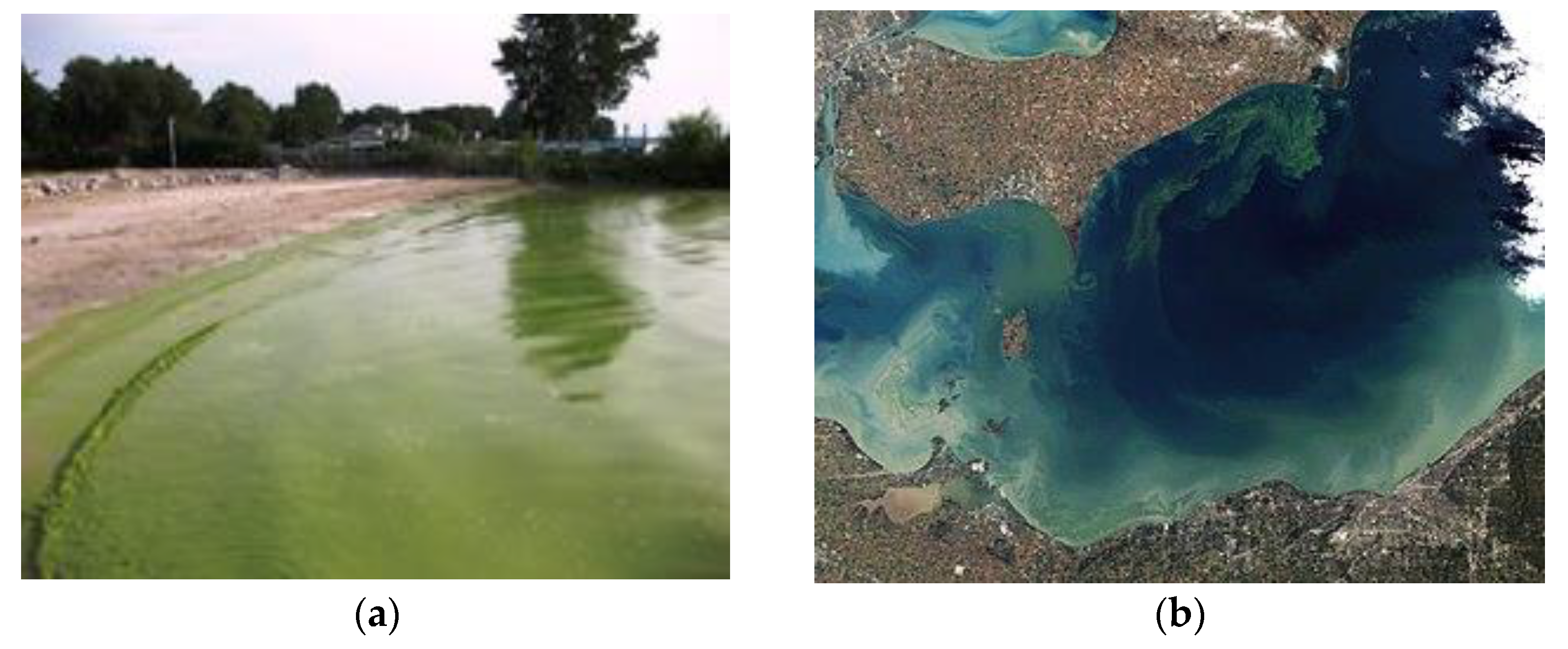
Figure 1.
Cyanobacteria (blue-green algae) blooms on Lake Erie in (a) 2009 and (b) 2011.

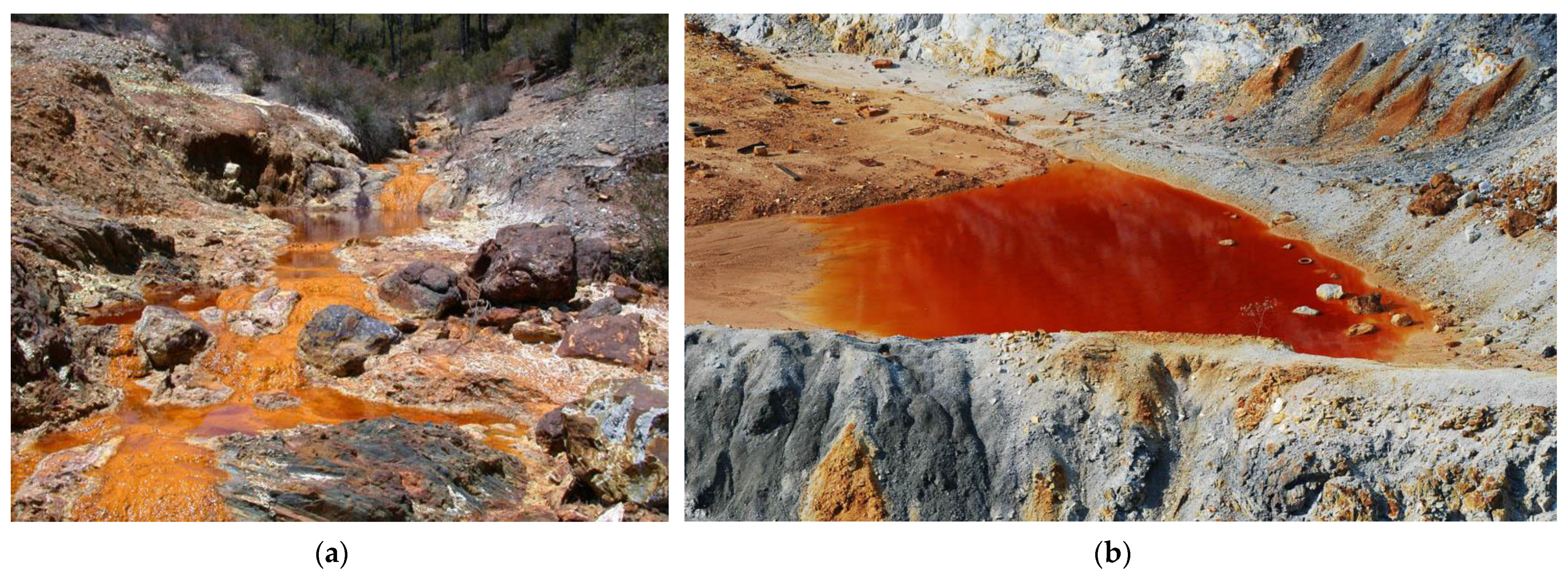
Figure 2.
(a) Rio Tinto, a river in South Spain, affected by mine drainage; (b) Acid Mine Drainage in Central Sweden as seen by Copernicus Sentinel satellites.
Figure 2.
(a) Rio Tinto, a river in South Spain, affected by mine drainage; (b) Acid Mine Drainage in Central Sweden as seen by Copernicus Sentinel satellites.

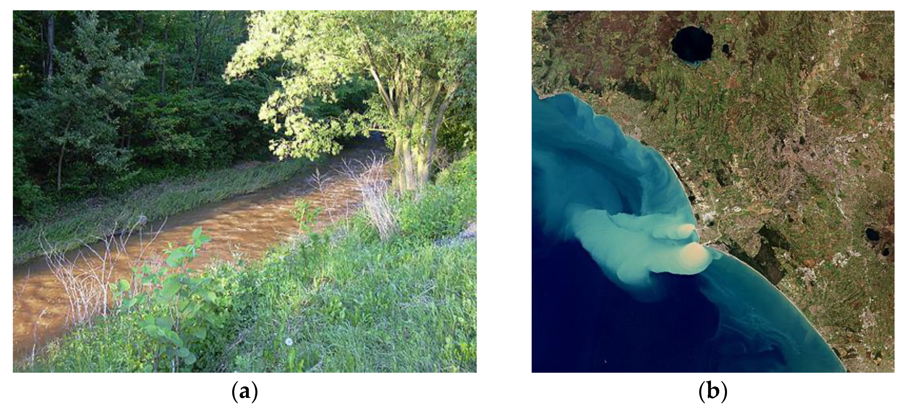
Figure 3.
(a) Sediment transport; (b) River discharging sediment.


Table 1.
Landsat 8, Landsat 9 Electromagnetic Spectrum Bands of Observation.
| Band | Spatial Resolution in Meters (m)— Observable Parameters 1 | Wavelength Nanometers (nm) |
|---|---|---|
| 1 | 30—coastal, aerosol, shallow water, coral, dust, smoke | 435–451 |
| 2 | 30—blue, aerosols, land | 452–512 |
| 3 | 30—green, aerosols, land | 533–590 |
| 4 | 30—red, aerosols, land | 636–673 |
| 5 | 30—infrared, aerosols, land | 851–879 |
| 6 | 30—infrared, vegetation | 1566–1651 |
| 7 | 30—infrared, vegetation | 2107–2294 |
| 8 | 15—high resolution grayscale | 503–676 |
| 9 | 30—cirrus, atmospheric correction | 1363–1384 |
| 10 | 100—thermal infrared, surface temperature, crop water use | 10,606–11,190 |
| 11 | 100—thermal infrared, surface temperature, crop water use | 11,500–12,510 |
Table 2.
Sentinel-2 MSI Electromagnetic Spectrum Bands of Observation.
| Band | Spatial Resolution in Meters (m)— Observable Parameters 1 | Wavelength Nanometers (nm) |
|---|---|---|
| 1 | 60—aerosols | 443 |
| 2 | 10—blue, aerosols, land parameters | 490 |
| 3 | 10—green, aerosols, land parameters | 560 |
| 4 | 10—yellow, aerosols, land parameters | 665 |
| 5 | 20—red, vegetation, land parameters | 705 |
| 6 | 20—infrared, land parameters | 740 |
| 7 | 20—infrared, land parameters | 783 |
| 8 | 10—infrared, water vapor, land parameters | 842 |
| 8a | 20—infrared, water vapor, land parameters | 865 |
| 9 | 60—infrared, water vapor | 940 |
| 10 | 60—infrared, cloud detection | 1375 |
| 11 | 20—infrared, land parameters | 1610 |
1 An adaptation from information provided on eoportal.org and sentinel.copernicus.eu (accessed on 27 March 2022).
Table 3.
Terra & Aqua MODIS Electromagnetic Spectrum Bands of Observation.
| Band | Spatial Resolution in Meters (m)— Observable Parameters 1 | Wavelength Nanometers (nm) |
|---|---|---|
| 1 | 250—aerosols, land | 620–670 |
| 2 | 250—aerosols, land | 841–876 |
| 3 | 500—aerosols, land | 459–479 |
| 4 | 500—aerosols, land | 545–565 |
| 5 | 500—aerosols, land | 1230–1250 |
| 6 | 500—aerosols, land | 1628–1652 |
| 7 | 500—aerosols, land | 2105–2155 |
| 8 | 1000—ocean color, biogeochemistry, phytoplankton | 405–420 |
| 9 | 1000—ocean color, biogeochemistry, phytoplankton | 438–448 |
| 10 | 1000—ocean color, biogeochemistry, phytoplankton | 438–493 |
| 11 | 1000—ocean color, biogeochemistry, phytoplankton | 526–536 |
| 12 | 1000—ocean color, biogeochemistry, phytoplankton | 546–556 |
| 13 | 1000—ocean color, biogeochemistry, phytoplankton | 662–672 |
| 14 | 1000—ocean color, biogeochemistry, phytoplankton | 673–683 |
| 15 | 1000—ocean color, biogeochemistry, phytoplankton | 743–753 |
| 16 | 1000—ocean color, biogeochemistry, phytoplankton | 862–877 |
| 17 | 1000—atmospheric water vapor | 890–920 |
| 18 | 1000—atmospheric water vapor | 931–941 |
| 19 | 1000—atmospheric water vapor | 915–965 |
| 20 | 1000—surface temperature, cloud temperature | 3.660–3.840 |
| 21 | 1000—surface temperature, cloud temperature | 3.929–3.989 |
| 22 | 1000—surface temperature, cloud temperature | 3.929–3.989 |
| 23 | 1000—surface temperature, cloud temperature | 4.020–4.080 |
| 24 | 1000—atmospheric temperature | 4.433–4.498 |
| 25 | 1000—atmospheric temperature | 4.482–4.549 |
| 26 | 1000—cirrus clouds, water vapor | 1.360–1.390 |
| 27 | 1000—cirrus clouds, water vapor | 6.535–6.895 |
| 28 | 1000—cirrus clouds, water vapor | 7.175–7.475 |
| 29 | 1000—cloud properties | 8.400–8.700 |
| 30 | 1000—ozone | 9.580–9.880 |
| 31 | 1000—surface temperature, cloud temperature | 10.780–11.280 |
| 32 | 1000—surface temperature, cloud temperature | 11.770–12.270 |
| 33 | 1000—cloud top altitude | 13.185–13.485 |
| 34 | 1000—cloud top altitude | 13.485–13.785 |
| 35 | 1000—cloud top altitude | 13.785–14.085 |
| 36 | 1000—cloud top altitude | 14.085–14.385 |
1 An adaptation from information provided by modis.gsfc.nasa.gov (accessed on 27 March 2022).
Table 4.
Corresponding Wavelengths for Water Quality Assessment.
| Event | Reflectance Color/Spectra | Satellite | Wavelengths | Additional Information |
|---|---|---|---|---|
| Algal Blooms | Blue/Green | Multi-sensor Approach with Landsat and Sentinel | 665 and 709 nm | Utilize algorithms and masks to remove vegetative influences |
| Acid Mine Drainage | Orange/Red | Airborne hyperspectral data, HyspIRI | 570–700 nm | Monitor during dry season; reference libraries can be useful for determining mineral mixtures |
| Suspended Sediments | Brown/Tan | Landsat TM Landsat OLI Sentinel-2 MSI | 700–800 nm *650 nm if less severe | Utilize multi-band linear regression models with site-specific coefficients |
Publisher’s Note: MDPI stays neutral with regard to jurisdictional claims in published maps and institutional affiliations. |
© 2022 by the authors. Licensee MDPI, Basel, Switzerland. This article is an open access article distributed under the terms and conditions of the Creative Commons Attribution (CC BY) license (https://creativecommons.org/licenses/by/4.0/).
Share and Cite
MDPI and ACS Style
Murray, C.; Larson, A.; Goodwill, J.; Wang, Y.; Cardace, D.; Akanda, A.S. Water Quality Observations from Space: A Review of Critical Issues and Challenges. Environments 2022, 9, 125. https://doi.org/10.3390/environments9100125
AMA Style
Murray C, Larson A, Goodwill J, Wang Y, Cardace D, Akanda AS. Water Quality Observations from Space: A Review of Critical Issues and Challenges. Environments. 2022; 9(10):125. https://doi.org/10.3390/environments9100125
Chicago/Turabian StyleMurray, Cameron, Albert Larson, Joseph Goodwill, Yeqiao Wang, Dawn Cardace, and Ali S. Akanda. 2022. "Water Quality Observations from Space: A Review of Critical Issues and Challenges" Environments 9, no. 10: 125. https://doi.org/10.3390/environments9100125
Note that from the first issue of 2016, this journal uses article numbers instead of page numbers. See further details here.