1. Introduction
Noise is an impactful pollutant that can lead to severe hearing implications when higher exposure levels are involved [
1,
2]. Even continuous exposure to moderate levels can result in nonhearing health effects [
3,
4,
5,
6,
7,
8,
9,
10] as well as repercussions in adolescents’ and children’s development [
11,
12].
Conscious of those criticalities, the European Union has formulated a three-step plan to mitigate noise. As a first step, European Union member states are advised to periodically control the noise exposure of citizens living in cities above 100,000 inhabitants or the areas in proximity to the main transport infrastructure such as roads, railways, and airports [
13]. This control phase is followed by a second phase of presenting the results of noise exposure to the public. Following this, the final stage deals with preparing and implementing action plans for noise mitigation. The three steps are repeated every five years. The control phase can be realized with the implementation of noise monitoring campaigns or by means of noise maps, which are often preferred as they are cheaper and easier to implement. The quality of the results of this first stage is crucial in defining action plans because an underestimation or overestimation of noise levels could lead to noise mitigation actions which are ineffective or unnecessarily oversized and expensive.
Relatively low levels of uncertainty (<3 dB) can be realized by validating noise maps in comparison to field measurements. However, noise map results are limited to the condition present during the observation period. The noise environment could have been changed during the 5 years between the two consecutive mapping intervals and, thus, citizens’ exposure to noise levels can be affected [
14]. Therefore, periodical checks on noise levels are suggested to avoid discrepancies between real noise levels and the predicted ones. From this perspective, noise monitoring networks offer the more effective alternative because they can continuously monitor noise levels and spot anomalous acoustic events, resulting in the capability to highlight noise level oscillations. Noise monitoring is mainly used for traffic [
15] or airport noise [
16,
17] and can allow for dynamic noise mapping [
18], seasonality analysis [
19], and traffic flow extrapolation through noise source recognition [
20]. Nowadays, cheaper alternatives to high-quality conventional noise sensors are being tested worldwide [
21]. The Environmental Noise Directive (END) classifies ports as industrial noise, but they are more likely a transportation hub that include a lot of different noise sources [
22]. Often, ports are also close to urban areas and, since their noise can reach long distances [
23], the monitoring of citizen’s exposure is critical.
Among the several research projects that focused on port noise [
24], the Interreg Maritime program concentrated its resources around the North Tyrrhenian Sea, conducing different studies focused on the definition of the state of the art and also on developing guidelines, with particular attention to noise mapping and the adequate acoustical characterization of noise sources [
25,
26,
27,
28]. The Interreg MON ACUMEN project focused on the monitoring and control of port noise through the realization of noise monitoring networks in the ports of Bastia, Cagliari, La Spezia, and Livorno. The aim of those monitoring networks is to allow port authorities to effectively manage and control noise emission in the port area, to inform citizens on the noise produced by the port, and to effectively identify the sources of noise criticalities, providing an indication for noise reduction actions. Noise monitoring results can also constitute a basis for future studies in the realization of port noise emission models in relation to the volume of different freights’ flux in the port area.
Effective noise monitoring must be performed in key selected points that can give precise indications of responsibility for noise emission in case of criticality or complaints from the public. This is especially true for airport noise, where the stations are mandatory. Moreover, it must recognize critical phenomena and react by producing alerts and/or recording additional information to be processed when reviewing the data. Moreover, it must be “continuous,” meaning that as much time coverage as possible must be provided. In the MON ACUMEN project, these aspects were addressed in the preliminary stage through the creation of noise maps and the subsequent analysis of the results in the form of a noise source predominance map (NSP) and intensive noise source predominance map (INSP) [
23]. Those maps were developed in order to identify areas where sources dominate over the other. In the identified areas, monitoring stations of the network, focused on a specific source, can be installed in the port. In this way, different sources are monitored independently from each other. Once the suitable locations have been identified, they will remain adequate if the internal organization of port activities remain unchanged. Thus, in the absence of a significant logistic rearrangement of the port, the condition will remain satisfied. Therefore, the noise monitoring networks were built based on a specific set of technical requirements specifically defined to guarantee the vigilance and security of the network [
29].
Reaching a sufficient level of monitoring continuity requires adequate reliability in the system, and scheduled and unscheduled maintenance needs to be carried out to ensure the upkeep of the system. There are several costs associated with this network maintenance activity, which must be carefully monitored in order to keep the network economically sustainable in the long term. A cost that is too high could cause inefficiency, leading to the decommissioning of the network. This scenario would be detrimental from two different points of view. First, the citizens would lose an important instrument to be informed on the noise situation around the port area. Second, the port authority would not be able to guarantee the sustainable development of port activities from the noise emission point of view. Thus, to ensure the economic viability of the network investment, the network performance needs to be evaluated from a technical and financial point of view. In other fields, this task is supported by the evaluation of key performance indicators (KPIs).
In line with these objectives, in the present work, a set of technical and financial key performance indicators (KPIs) are presented that would support the stakeholders to evaluate the performance of the existing monitoring system and drive the installation of new ones. As a case study, the monitoring networks installed in the ports of Cagliari, La Spezia, and Livorno are evaluated with the developed KPIs.
The developed roadmap can easily be implemented for evaluating the performance of the installed noise monitoring networks in agglomerations and/or close to main transportation infrastructures such as roads and railways.
2. Materials and Methods
In this section, the KPIs defined to allow the evaluation of the network’s technical and financial performance are described. The evaluation of the performance of noise monitoring networks is unique, and the present work focuses on KPIs for environmental monitoring networks based on experience gained during noise monitoring campaigns and environmental legislations in this domain.
2.1. Technical KPIs
Technical KPIs are partially inspired by the air quality monitoring network defined in Appendix 1 of the European Directive 2008/50/CE [
30], which sets the minimum requirements to consider the results of a monitoring network valid for different air pollutants. In particular, at least 90% of the data must be acquired, with a consequent maximum allowable downtime of 10%. Those percentages do not include losses of data due to the regular calibration or the normal maintenance of the instrumentation. According to this guideline, the operability threshold for a sufficient rating was set to 90%. Then, as reported in
Table 1, three classes of performance to provide more granularity in the performance evaluation, corresponding to the 90%, 94%, and 98% operability thresholds, were defined, respectively.
Thus, the evaluation of the technical performance primarily focuses on the percentage of system downtime hours. The lower this percentage is, the better the network performance ratings will be. However, a minimum percentage of downtime will be inevitable due to extraordinary maintenance activities, making the 100% uptime a theoretical limit. Identifying the reasons behind the negative performance of the network would be possible by recording the cause of the downtimes; thus, one can compare the performance of noise monitoring networks installed in different places. In this way, the best management strategies can be identified and adopted in the other networks, leading to the definition of best practices to achieve the minimum downtime possible.
Besides the ordinary or extraordinary maintenance downtimes, noise monitoring is also affected by weather conditions. Indeed, any outdoor noise measurement is invalid in the presence of any precipitation (rain, snow, or hail) or a wind speed higher than 5 m/s. Thus, downtimes will also occur for meteorological reasons. Although this downtime depends on external factors, it is important to take note of their causes to identify improvement potential in terms of the positioning of the network nodes in relation to the local weather conditions. An example will be discussed in the case of the Cagliari monitoring network in the subsequent paragraphs.
The list of information to be gathered by the network administration to perform a network performance evaluation is as follows:
The number of hours of inactivity of the system as a whole.
A description of the main causes of system downtime, including:
The percentage of downtime due to routine maintenance, automatic local calibration, and the periodic calibration of instrumentation in certified laboratories.
The percentage of downtime due to acquisition downtime and extraordinary maintenance (a description of the maintenance reasons must be also provided).
The percentage of downtime due to adverse weather conditions.
The percentage of downtime due to power distribution network and communication network malfunctions.
The number of hours of downtime of the data consultation web services, specifying:
The percentage of downtime due to the scheduled maintenance of the information technology (IT) infrastructure;
The percentage of downtime due to system downtime and to the extraordinary maintenance of the IT infrastructure.
The percentage of hours due to exogenous factors, indicating the major critical issues.
2.2. Financial KPIs
The importance of a high level of financial performance ensures the medium- and long-term operativity of the network and the continuity of the service provided to stakeholders, including the citizens. The costs of maintaining and operating the network (hardware and software) must be sustainable in the long term. It is to be noted that as no revenue is generated, the direct and indirect associated expenditures are considered in formulating the financial KPI. The information required from individual port administrators to judge financial performance are the following expenses incurred in a semiannual period:
For maintenance:
The ordinary maintenance of instrumentation, such as periodically certified calibration.
The extraordinary maintenance of instrumentation, such as the replacement of damaged components.
The ordinary maintenance of the IT infrastructure, such as security updates.
The extraordinary maintenance of the IT infrastructure, such as recovery from storage failure.
For network management personnel costs (including dissemination of results):
Management:
Power costs (including only estimates).
Network expenses (data sim).
Storage expenses (SD cards, HDDs, etc.).
The dissemination of results (materials for public presentations).
Website maintenance costs.
Purchase and installation costs.
As no direct income is expected to come from the installation of a noise monitoring network, an indirect financial advantage is expected because, in the absence of the noise monitoring network, the lack of emission control could lead to an increase in noise levels, which could lead to a total or partial interruption to port activities, leading to financial losses. Therefore, from the cost–benefit assessment perspective, those losses should be compared with the network maintenance cost, management cost, and infrastructure investment costs to evaluate the advantages of the noise monitoring network. With this objective, the following information was requested from the relevant port authorities:
The number of threshold value exceedances.
The average value of expenses incurred by the port authority attributable to the handling of citizen complaints.
The average annual number of complaints filed by the citizens.
The possible lost hourly/daily revenue that could result from the suspension of port activities during daylight hours (between 06:00 A.M. and 10:00 P.M.) and during the night hours (between 10:00 P.M. and 06:00 A.M.) for each type of activity in the port, such as commercial, passenger, industrial, oil and gas, and ship building.
The estimated possible losses connected to activity interruption were provided by the port authorities, but it is difficult to precisely estimate the KPIs using these; apart from these, no data on threshold exceedance were provided, which needs further investigation.
It is worth mentioning that depreciation/amortization should be also included as a cost. In the specific case of the monitoring systems evaluated in the present work, amortization was not considered because the purchase of the instrumentation was carried out under a European project. Indeed, it is common practice that, if some particular requirements are met, the equipment acquired within European projects will not be subjected to depreciation.
3. Results Obtained from the Monitoring Systems
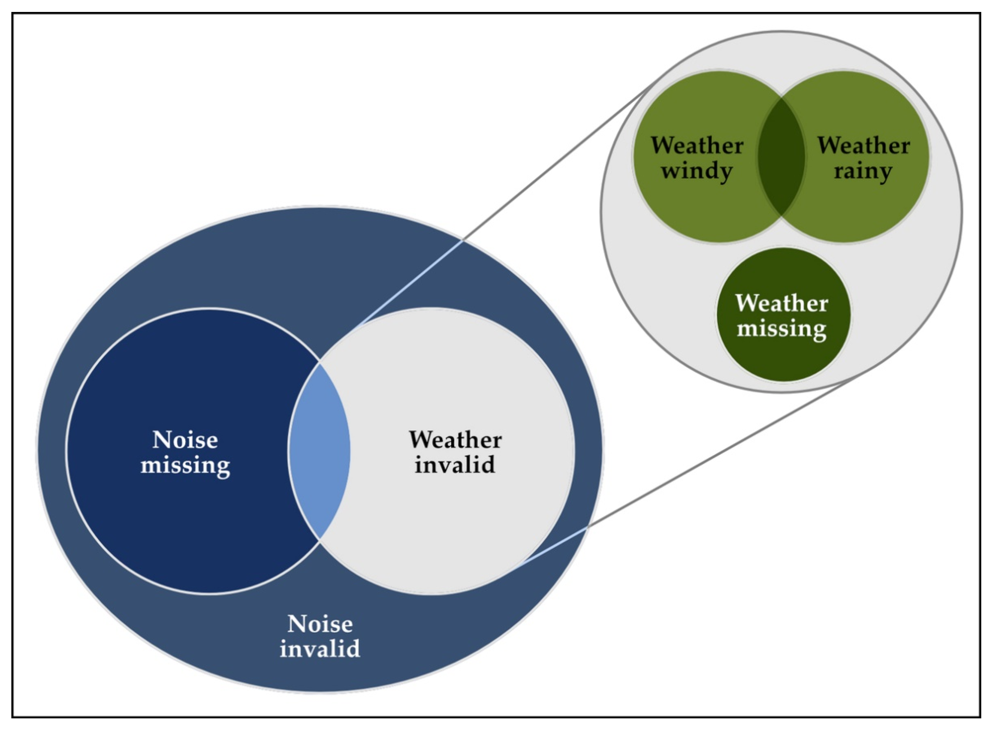
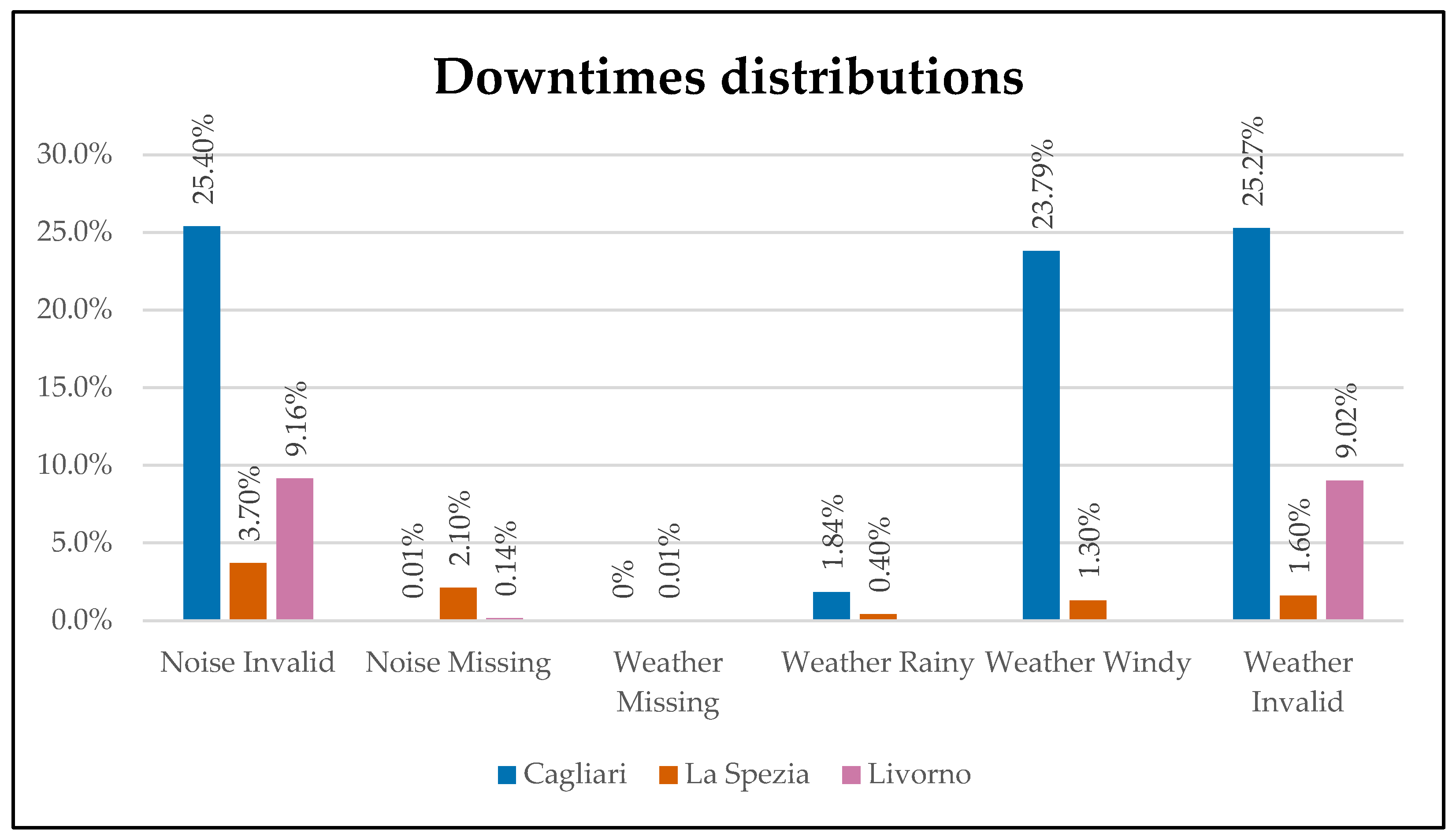
In this section, the results obtained from the monitoring systems installed in the Italian ports of Cagliari, La Spezia, and Livorno are reported. The results are relative to the first period of operation of the networks. The terminology used is the following:
“noise invalid”: total acoustic data missing due to interruptions to acquisition or invalid weather data.
“noise missing”: acoustic data missing due to interruptions to the SPL meter acquisitions.
“weather invalid”: total weather data invalid due to rainy or windy weather or to an interruption to weather acquisition.
“weather missing”: missing weather data due to an interruption to weather acquisition.
“weather rainy”: weather data identified as rainy, according to the specified criterion.
“weather windy”: weather data identified as windy, according to the specified criterion.
A graphical representation is provided in
Figure 1.
3.1. Technical KPIs’ Results
In the present section, the technical KPIs evaluated on the three ports are presented along with a short description of the networks.
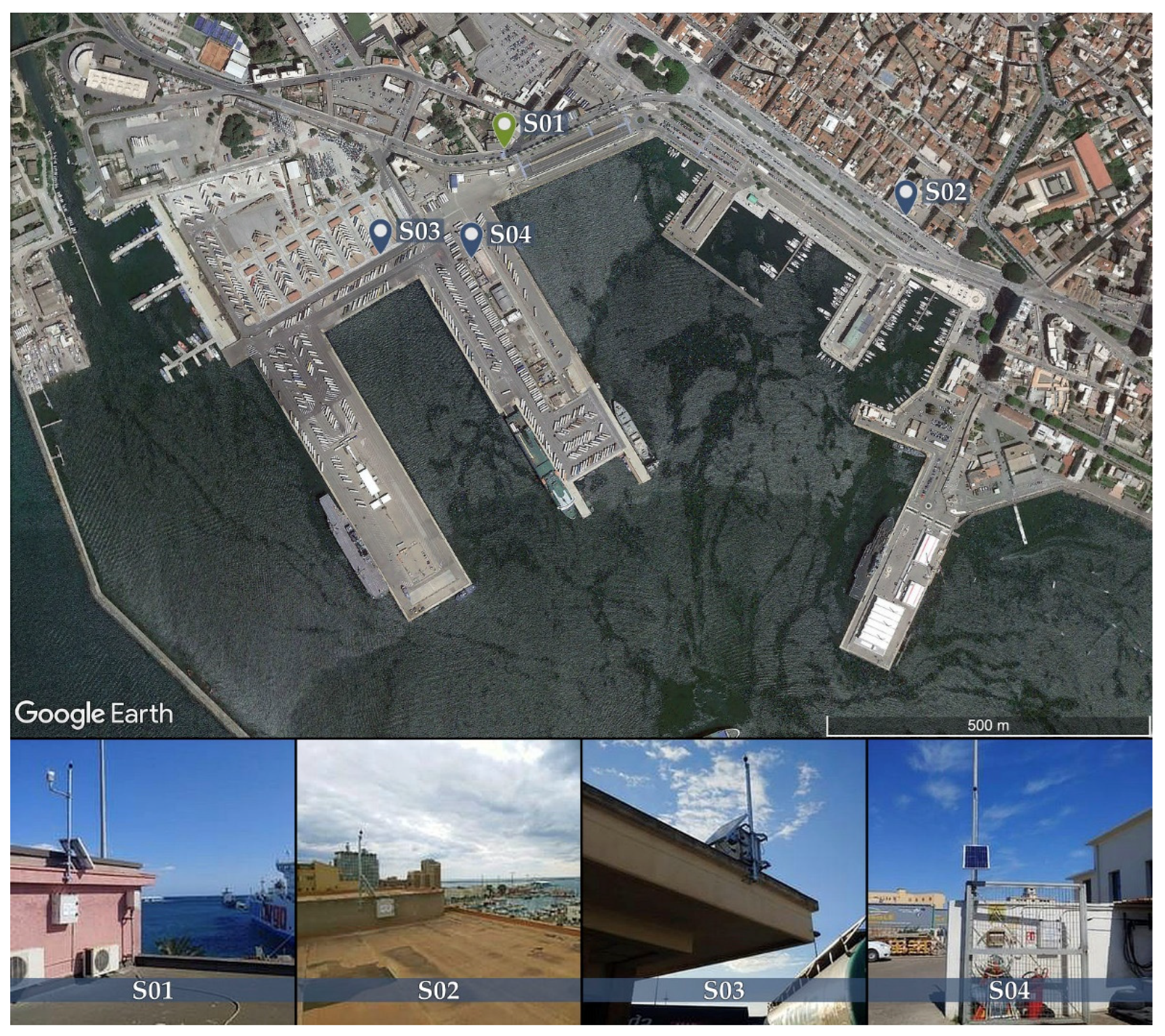
3.1.1. Port of Cagliari
The network installed in the Port of Cagliari comprises four noise monitoring stations with “Class 1” [
31] sound pressure level (SPL) meters (“Fusion” from “01dB”). Out of these, one of them (S01) integrates meteorological sensors (VAISALA WXT 536) All the monitoring stations are installed with an IP65 enclosure and are provided with a redundant power source, including the connection to the electrical network, a battery, and a photovoltaic panel. The positioning of the monitoring stations is reported in
Figure 2.
The calculation of the KPIs was based on the period from 22 April 2021 at 06:00 A.M. to 27 June 2021 at 06:00 A.M., for a total of 66 days, amounting to 1584 h of monitoring for each monitoring station and 6336 h in total. The interruption duration for individual interruption sources is presented in
Table 2, while the overall results are reported in
Table 3. During the observation period, downtimes due to SPL meters were caused only by routine maintenance operations such as short stops and restarts of the acquisition, for a total time of less than one hour. Additionally, no extraordinary maintenance or failures were reported and web services reported no such interruptions.
Based on the observation, the uptime not related to adverse weather conditions was 99.9% and, therefore, the system performance can be rated as “Excellent”. However, the large percentage time affected by adverse weather conditions was alarming, as it rendered the system inoperative for more than 25% of the observation period.
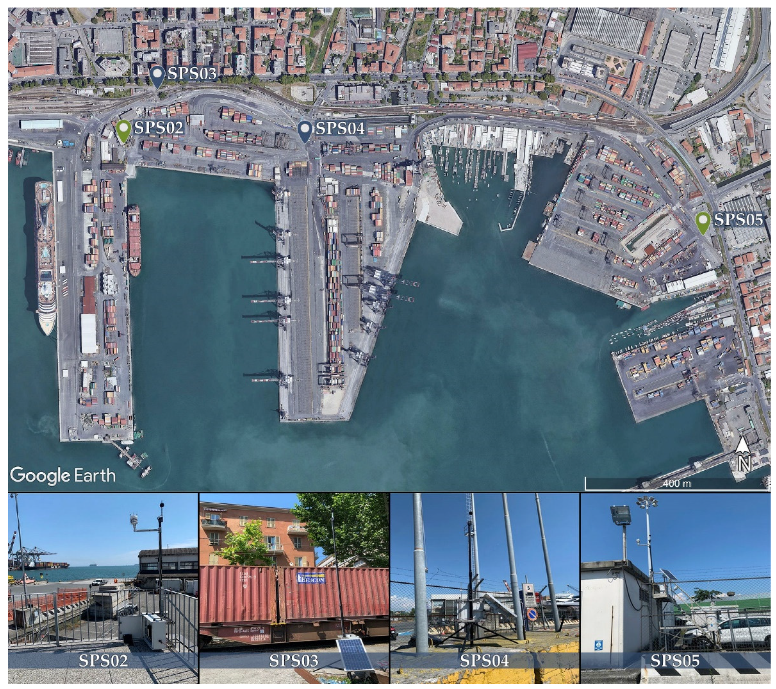
3.1.2. Port of La Spezia
The Port of La Spezia’s network is made of four noise monitoring stations with “Class 1” SPL meters, and two of them integrate a meteorological data acquisition mechanism (
Figure 3). The employed SPL meters are “CUBE 4G” from “01dB”, equipped with a “DMK01” microphone, enclosed in an IP65 enclosure and powered by a battery and an attached photovoltaic panel. The weather data are acquired from a “WXT536” station from “VAISALA”.
The evaluation of the performance took place over two separate but consecutive periods. The first was 37 days, from 29 May at 06:00 A.M. to 5 July at 06:00 A.M., in the year 2021. The monitoring of noise levels and, thus, the analysis of acoustic data were performed in this period. In total, 888 h of monitoring was observed for each unit for a total duration of 3552 h altogether. Complete weather-related inactivity details were made available from this period.
The next period, nine days long, from 5 July 2021 to 13 July 2021, was provided without the validation of the acoustic data. Therefore, downtime due to adverse weather was not available in this interval. Nevertheless, the port authorities reported the absence of extraordinary or routine maintenance; thus, it was possible to calculate the percentage of activity related only to technical causes for 4416 h in total.
The number of downtime hours is shown in
Table 4, and the overall results are reported in
Table 5. The overall percentages for each parameter are also shown. As can be seen, the greatest cause of outages can be traced to the extraordinary maintenance of the SPL meter. Among the meteorological causes, wind was the most frequent.
Some extraordinary maintenance operations were conducted during the monitoring activities regarding the SPS03 and SPS04 monitoring stations. Specifically, for the SPS04 station, the installation of a 4G modem for data transmission was carried out on 10 June 2021 for a total of 18.2 h. For the SPS03 station, some extraordinary operations were carried out in the first days of monitoring related to the installation and configuration of the system, which resulted in downtimes from the 29 to the 31 of May 2021, for a total of 56.6 h. The total downtimes due to extraordinary maintenance are estimated to be 72.8 h, accounting for 2.0% of the monitoring hours during the observation period.
During the monitoring activities, SPL meter calibrations were performed on June 18 and June 24 in the year 2021. Similarly, SPS03 and SPS05 were calibrated on 19 June 2021 and SPS02 and SPS04 were calibrated on 24 June in the same year. The calibration activities resulted in a few minutes of interruption to the acquisition, which is considered a routine maintenance activity. The other interruptions were due to brief stops and restarts of the SPL meter acquisitions due to normal system operation.
Considering the absence of interruption due to the extraordinary maintenance of the SPL meters in the second observation period, the total observation time can be considered equal to 4416 total hours of monitoring, while the extraordinary maintenance downtimes were as long as 72.8 h. Therefore, the uptime of the network results equaled 98.3%, which can be rated as excellent.
Regarding the web platform, no interruptions due to the ordinary or extraordinary maintenance of the IT infrastructure were reported during the observation period.
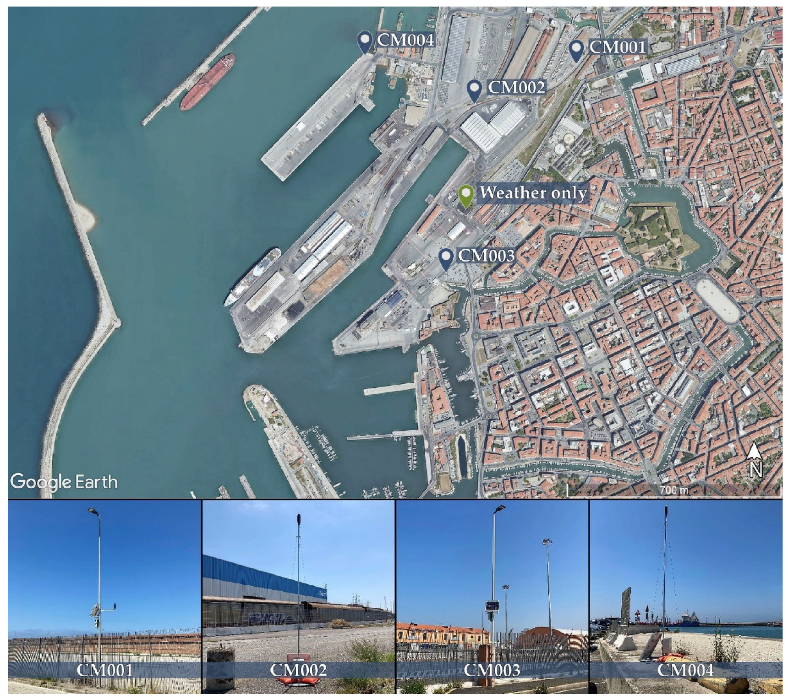
3.1.3. Port of Livorno
The noise monitoring network installed in the Port of Livorno is composed of four noise monitoring stations with “CR:191IT” “Class 1” SPL meters from CIRRUS, equipped with a MK224 microphone and enclosed in an IP56 box. The power is provided by the combination of a battery and a photovoltaic panel. The network is integrated with the pre-existent environmental monitoring network that also provides the weather data. The monitoring points and the weather monitoring are reported in
Figure 4. The interruption duration for individual interruption sources is presented in
Table 6, while the overall results are reported in
Table 7. The total duration of the monitoring network’s activity was 42 days, from 14 June 2021 to the 26 July 2021, amounting to 4051.56 h of monitoring.
The downtime due to routine maintenance was found to be about 5 min for each monitoring station, regarding only calibration operation. The percentage of downtime due to acquisition downtime or extraordinary maintenance operation was found to be about 5 h on one SPL meter due to system upgrade operation and several minutes on each of the other three SPL meters. The downtime was due to data transmission routines concerning the internet of things (IoT) being involved. No downtime for the IT infrastructure or the web platform was reported.
3.1.4. Comparison
In
Figure 5, a graphical comparison between the downtime occurrences for the three ports is reported. “Noise missing” percentage, which is representing the mere technical performance, is very low for the three ports, but higher percentages of “noise invalid” were reported due to the contribution of the “weather invalid” indicator. The Port of Cagliari emerged as having the highest incidence of adverse weather conditions, while Livorno also showed a relatively high incidence, but in any case, they were below the threshold of 10%. For Livorno, no details on the contribution of rainy and windy weather were provided by the port authorities.
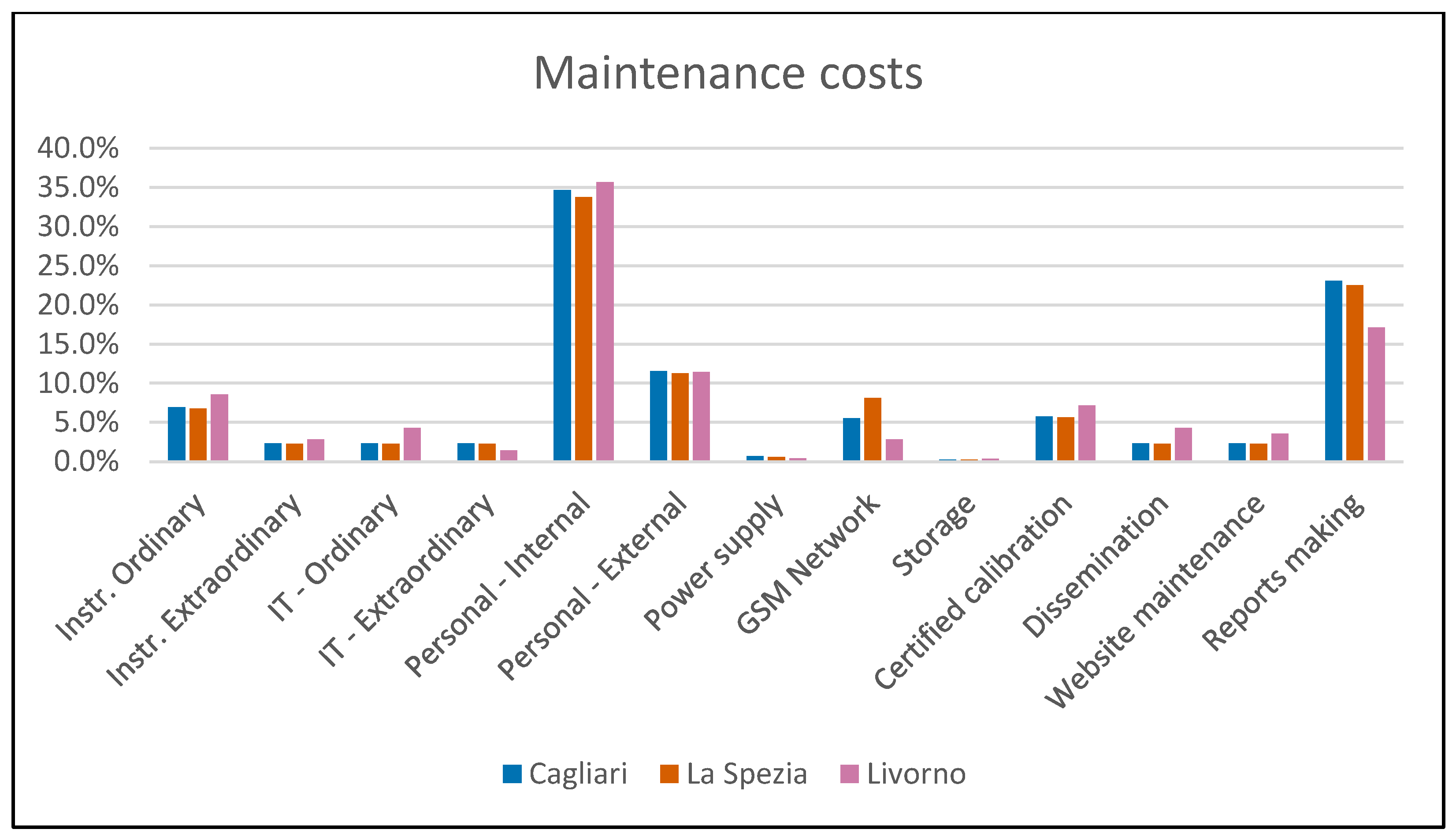
3.2. Financial KPIs
In this section, we report and compare the financial KPIs related to the monitoring networks. In
Table 8, all the estimates provided by the ports on the expenses to be incurred annually for the maintenance of the monitoring systems are reported. In
Figure 6, a comparison is also provided. The annual expenditure value is estimated to be, on average, just above EUR 4000.00 per monitoring station.
In
Table 9, on the other hand, the total investment costs faced by port authorities for the implementation and commissioning of the systems are reported. An estimate of the cost of installing a hypothetical “minimal” monitoring system consisting of an SPL meter and a weather station amounts to EUR 28,000.00. The addition of a second noise monitoring station or weather station would result in an average investment of an additional EUR 13,317.33 and EUR 3461.50, respectively.
In order to assess the cost–benefit ratio, some data were requested from the port authorities such as the average value of expenses incurred by the port authority, attributable to the handling of citizen complaints, or the average annual number of complaints submitted. An estimate of the possible lost hourly/daily revenue that could result from the interruption of port activities during daytime hours (between 06:00 A.M. and 10:00 P.M.) or night-time hours for each type of activity in the port was also requested. Indications on the economic benefits and/or economies guaranteed by the infrastructure were provided by the Port Authority of Livorno only, so it was not easy to calculate a representative cost–benefit ratio for the whole cooperation area.
The Port Authority of Livorno states that it does not incur any expenses for handling the exposures; however, based on the annual gross domestic production (GDP) of the port activities, a one-day interruption to port operations would result in substantial losses in terms of GDP, specifically as follows:
For the industrial/commercial sector, up to about EUR 3,000,000.00.
For the tourist/passenger sector, about EUR 90,000.00 on average.
It is to be noted that the values mentioned above could be affected by the season, i.e., they could be considerably higher in the summer period due to the concentration of flows.
In
Figure 7, a comparison between the investment expenditure distribution for the three ports is also reported.
4. Discussion
In this section, an analysis of the performance of the three different monitoring networks is presented. Therefore, data on total monitoring hours, downtimes, and corresponding percentages for all ports are summarized in
Table 10.
The performance of the installed monitoring systems was assessed as excellent from a purely technical point of view; however, the length of the observation period of 65 days did not allow for a definitive assessment. A future evaluation should be carried out with at least one year of operation for all the networks. The reliability of the IT infrastructures, and in particular the web interface, should be tested after the public release of the websites and with steady-state web traffic. Indeed, no tests of the resilience of the web infrastructure with multiple and simultaneous consultations were reported. Based on the available data, no service interruptions were reported.
Different considerations could be made regarding the total operability of the networks. In the case of the Port of Cagliari, weather conditions made 25% of the recorded data unusable, which is a very high percentage considering that the monitoring took place during the summer period. The most impactful parameter was the wind, which too often exceeded the 5 m/s speed threshold allowed by Italian law.
Considering the location of the meteorological station on the top of a building, there is a possibility that better weather could be measured going closer to the ground. Therefore, an investigation is recommended to evaluate the installation of a second weather station to monitor the windiness at a lower height. In the first instance, it would be useful to install a second weather station in one of the harbor’s two stations which are located below 4 m elevation.
On the other hand, the wind conditions experienced by the fourth monitoring station, located on top of the Sardinia Region building, could be represented with sufficient accuracy by the current weather station. In the fall, winter, and spring periods, the frequency of adverse weather conditions could increase due to the rain factor. Therefore, a deeper study would be crucial to achieve the highest possible effective system operability. In fact, maintaining the current operability would consist of the loss of an entire quarter of monitoring.
Similarly, the downtime rate due to adverse weather conditions was found to be about 9% in Livorno. By analyzing the monitoring period, it can be assumed that precipitation had a marginal influence compared to wind, but the contribution of the two causes was not reported in detail.
The Port of La Spezia was found to be less prone to disruptions due to weather, with a downtime rate of less than 2%. However, the percentage of downtime due to extraordinary infrastructure maintenance led to an initial rating of good. In the second period, no such downtime was observed and the percentage dropped to 1.6%, leading to a rating of excellent. Some interventions on the monitoring stations in the system set-up phase had an important influence, considering the short duration of the observation period. Extending the observation period, the performance will most likely align with that of the other two ports. This further consideration underlines how the observation periods were too short to make a definitive assessment, from both a weather and technical issue perspective.
Regarding the financial performance, the maintenance costs appeared to be low (less than EUR 5000 per year per monitoring station). Costs were estimated based on a relatively short period, and this value can only be an estimation subject to variations. Moreover, it was difficult to make an objective cost–benefit evaluation since no indications were provided by all ports on the economies allowed by the presence of the network. However, the indications provided by the Port of Livorno in this regard show how investing into a monitoring station requires relatively very little investment if compared to the potential day of activities lost due to the stops required by high noise levels. This information should be considered as a pure estimate and should be further investigated.
Nonetheless, the overall picture that emerged brings out the huge gap between the investment costs and maintenance costs of the infrastructure and the possible losses in GDP due to a single day of disruption of the port activity. Based on the dimension of the port in terms of traffic flow, the losses of GDP could be a detriment, not only to the port but also at the national level. The installation of noise monitoring systems in the port area enables the real-time management and control of port activity, producing advantages not only for the health of the citizens, but also for the industrial and commercial activity of the countries directly and not directly connected to the port.
5. Conclusions
European legislation requests the periodic control of citizens’ exposure to noise levels through the realization of monitoring campaigns or noise mapping. The latter, although more practical to be realized, provides a representation of the reality that is limited to the time of observation. Therefore, a more frequent evaluation of noise emission of the main noise sources is recommended.
Noise monitoring networks are suitable candidates for this task, allowing the continuous control of emission and, thus, of citizens’ exposure. On the other hand, there is a small possibility of them being widely adopted for such as task without an objective cost–benefit evaluation, and for this purpose, the definition of an adequate set of key performance indicators (KPIs) is crucial.
With the aim of evaluating the cost–benefit ratio of the implemented port noise monitoring networks, a set of technical and financial KPIs were defined. The KPIs were, thus, described, evaluated, and reported in the present work. As a test case, data were retrieved from the monitoring station installed in port areas during the MON ACUMEN Interreg project, but its application can be expanded to all noise monitoring, especially for airport noise.
From the results which emerged, from a purely technical standpoint, a high level of operativity can be reached with the current technology. Extending the analysis to the weather’s influence on operability, it can be stated that a lot of attention must be pointed towards the positioning of the monitoring stations and the evaluation of the minimum number of weather stations required to adequately represent weather conditions for all the monitoring stations.
The financial KPI evaluation highlighted a relatively low cost of investments required to build the network and relatively low costs of maintenance: less than EUR 5000.00 for monitoring stations per year. These costs, in the case of ports, must be compared with the potential loss connected to interruptions (or limitations) to port activities due to complaints and exceeding noise limits. For the other main noise sources such as roads, railways, airports, and industrial plants, analogous considerations can be made.
Therefore, the defined KPIs and the presented results could constitute an important instrument for decision makers evaluating the possibility to realize a noise monitoring network to control noise emission and citizens’ exposure, and a standardized evaluation method for the technical and financial performance of noise monitoring networks already in action.
Considering the relatively small observation period, the evaluation of performance needs to be performed over longer observation periods in order to verify the initial results, and further investigations should be performed when new data are available.


