Stochastic Approach for 2D Superficial Seismic Amplification Based on Quad4M; City of L’Aquila (Italy) Test Case

Abstract

The values of the physical–mechanical properties of any soil are affected by uncertainties both due to experimental measurements and the impossibility of knowing them, in detail, at every point of the spatial domain. Accordingly, this work focuses on uncertainty in shear wave velocity (V_s) and its impact on the seismic response. The Monte Carlo method, based on pseudo-random number generation, was selected. To understand which random distributions could identify the site’s real conditions, the Fourier spectrum frequencies were calculated for each realization and were compared with the predominant natural site frequency. The experimental range data were used to calculate the spectral average acceleration and the horizontal amplification factors. The simulations were performed and interpreted by a modified version of VisualQ4M software based on 2D Quad4M, including the generation of pseudo-random numbers and pre- and post-data processing. A site at a small scale, in the territory of the city of L’Aquila (Italy), was selected as the test case. This paper demonstrates, from a numerical point of view, that both a simple local topographic modification due to excavation and the uncertainties of the numerical values, even of the shear wave velocity alone, can have an important impact on the local seismic amplification.

1. Introduction

In recent years, particular attention has been paid to the local seismic amplification phenomena, intensifying the geological studies of the territories and the soils’ seismic characteristics to understand the causes that can trigger seismic waves’ surface focalizations [1].

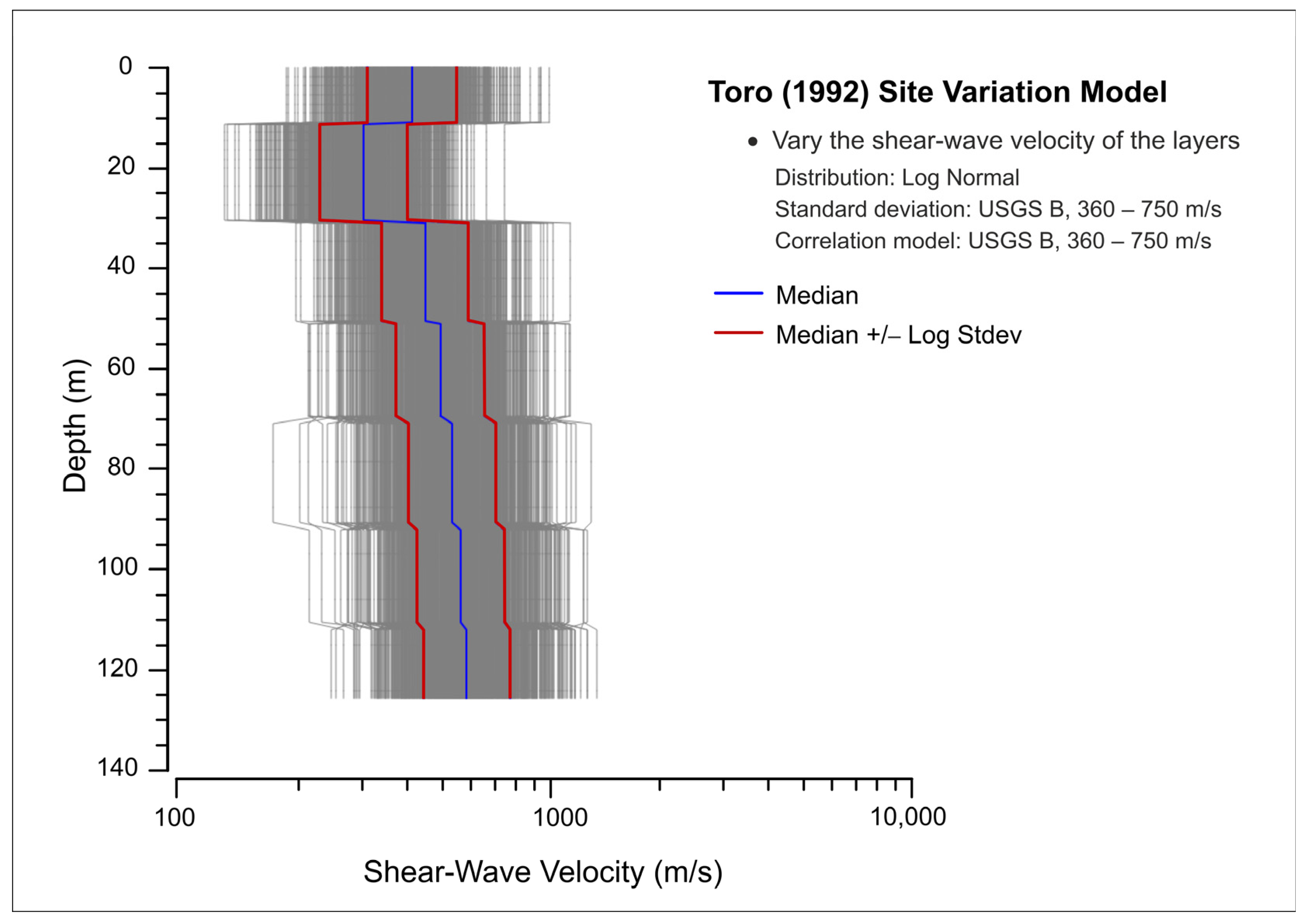
The numerical estimates of the surface seismic amplification are influenced by various factors, including the selected analysis method, the dynamic properties of the soil, the input motion, and the shear wave velocity profiles $V_s$. In this paper, in order to introduce a stochastic approach, the $V_s$ parameter was selected as a random parameter [2]. The $V_s$ can be evaluated with various geophysical methods (active and/or passive) or through empirical correlations [3]. Currently, engineering design codes have few guidelines regarding the inclusion of $V_s$ numerical uncertainty values for performing site response analyses. The uncertainties in the definition of the shear wave velocity can generate a numerical seismic response that is not always representative of the real surface amplifications. A common practice is the single deterministic analysis, using an average $V_s$ value for each, eventually multiple, layers. However, this kind of approach does not commonly guarantee a correct and, as far as possible, complete estimate of the implications due to the variability of the selected geotechnical parameters. Accordingly, in this paper, the probabilistic method, for which each physical parameter can be assumed as a function of a pseudo-random variable $U_{RND},$ was assumed. All compilers (Fortran, C++, Python, etc.) use default algorithms which, based on an internal clock and on an extremely long series of numbers, even with 10³⁶ elements, are able to select numerical values that are not completely random, and for this reason, they are called “pseudo-random” numbers.

Currently, a large international bibliography describes in detail the characteristics of the stochastic method applied to seismic amplification. An attempt to couple Probabilistic Seismic Risk Analysis and seismic micro-zonation, two of the most important components of seismic risk mitigation strategies, has been discussed in [4]. In the article [2], for the stochastic study of seismic risk, the variability of the $V_s$ was considered, and in [5], the effects resulting from the choice of three different ways of considering the $V_s$ were discussed. In [6], the Monte Carlo method was applied. The parameters that substantially influence the surface seismic amplification depend on the deformation in a non-linear way [7] (among many others). Accordingly, a technique to avoid the complexity of full non-linear numerical approaches has been proposed in [8] called “The Equivalent-Linear Method”. By this approach, a pseudo iterative linear analysis is performed, with some initial values assumed for damping ratio and shear modulus. The maximum cyclic shear strain is recorded for each element and used to determine new values for damping and modulus by reference to laboratory-derived curves that relate damping ratio and secant modulus to the amplitude of cycling shear strain.

Some empirical scaling factor is usually used when relating laboratory strains to model strains. The new values of damping ratio and shear modulus are then used in a new updated numerical run. The whole process is repeated several times until there are no further changes in properties. At this point, it is said that “strain-compatible” values of damping and modulus have been found, and the simulation using these values is representative of the response of the real site.

It is important to note that, to introduce stochastic variability in numerical modeling, there are two main commonly used techniques, the Spectral Approach [9] and the Monte Carlo method, which is more time-consuming, but more realistic.

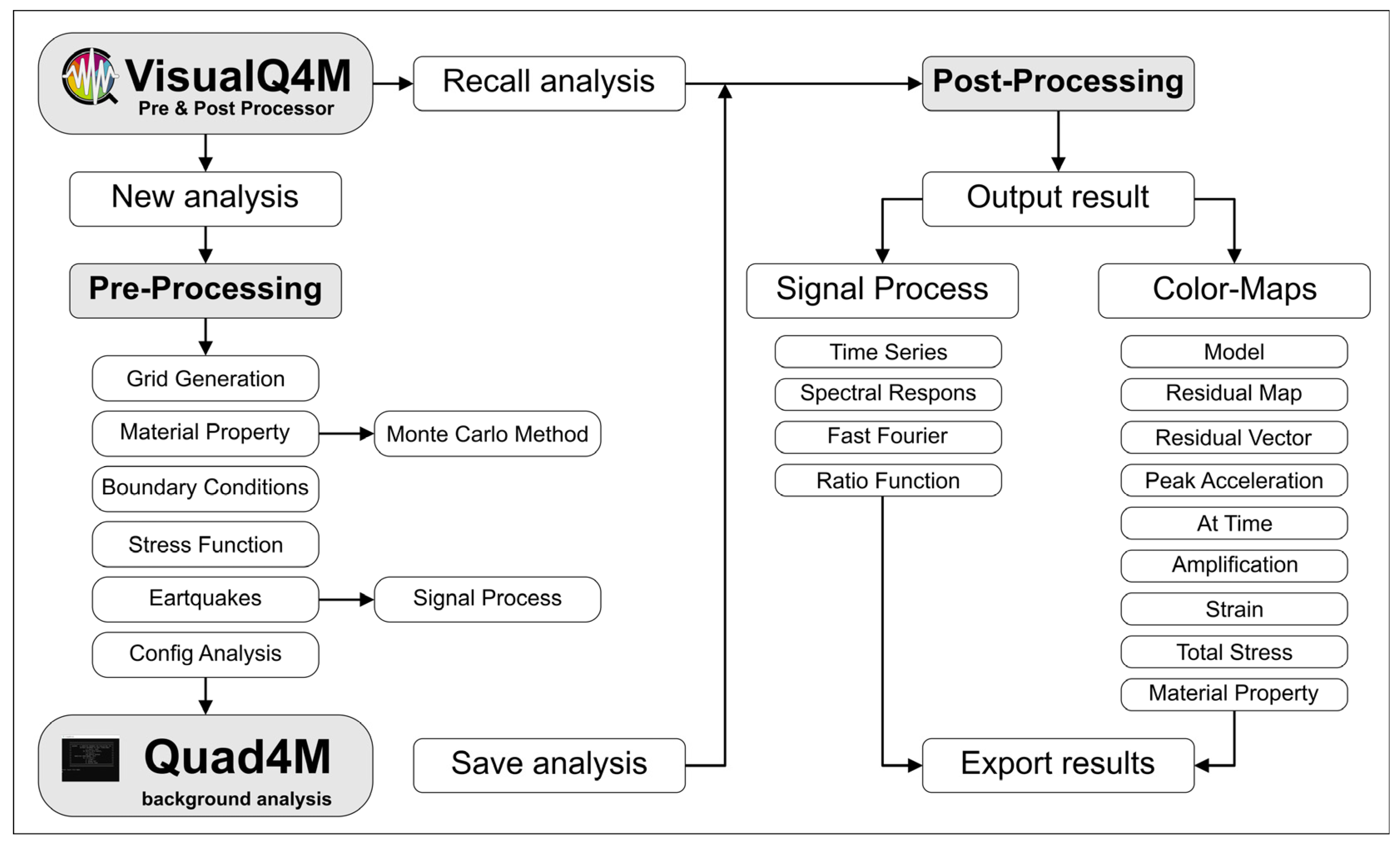
In the practice of engineering modelling, but also in research activities, a commonly internationally used software is the Quad4M [10], based on the 2D finite element method. The non-linearity of the soil is considered by “The Equivalent-Linear Method”. However, the parameters are entered in a deterministic way. To overcome this aspect, VisualQ4M, a new software (www.visualq4m.com, “URL (accessed on 16 January 2023)” [11], was developed, including a graphical user interface (GUI) for the pre- and post-processor with functionality and visual command able to generate, with excellent accuracy, geometric models suitable for the Quad4M program. The new software, selected to perform simulations discussed in this paper, manages all the seismic analyses in a single integrated interface to perform a complete 2D Quad4M simulation, producing various color-map results and spectral responses, as well. In addition, the selected software allows for the automatic performance of the Monte Carlo approach, even with a distribution of random values defined by the user, for example, variables with depth.

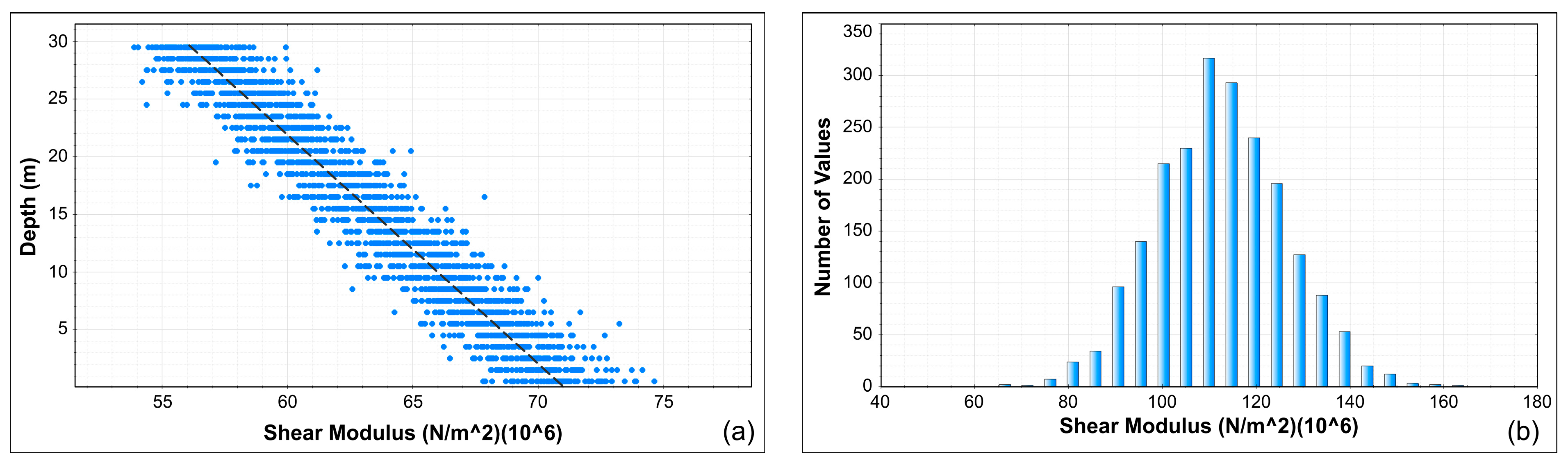
Accordingly, the Monte Carlo approach was applied to analyze different possible realizations of the system under consideration, resulting from different, but possible, statistical distributions of the $V_s$ parameter, selected as a random variable.

The spatial domain was discretized by geometric elements of varying size depending on location, but whose minimum dimension was no less than one meter. Therefore, in order to simplify the approach, we assumed that the autocorrelation and cross-correlation scales were, for the system under consideration, below 1.0 m, thus avoiding the elaboration of a spatially random distribution of geotechnical parameters using approaches such as those developed by Metropolis–Hastings [12] and others [13,14]. This option will be implemented in future activities.

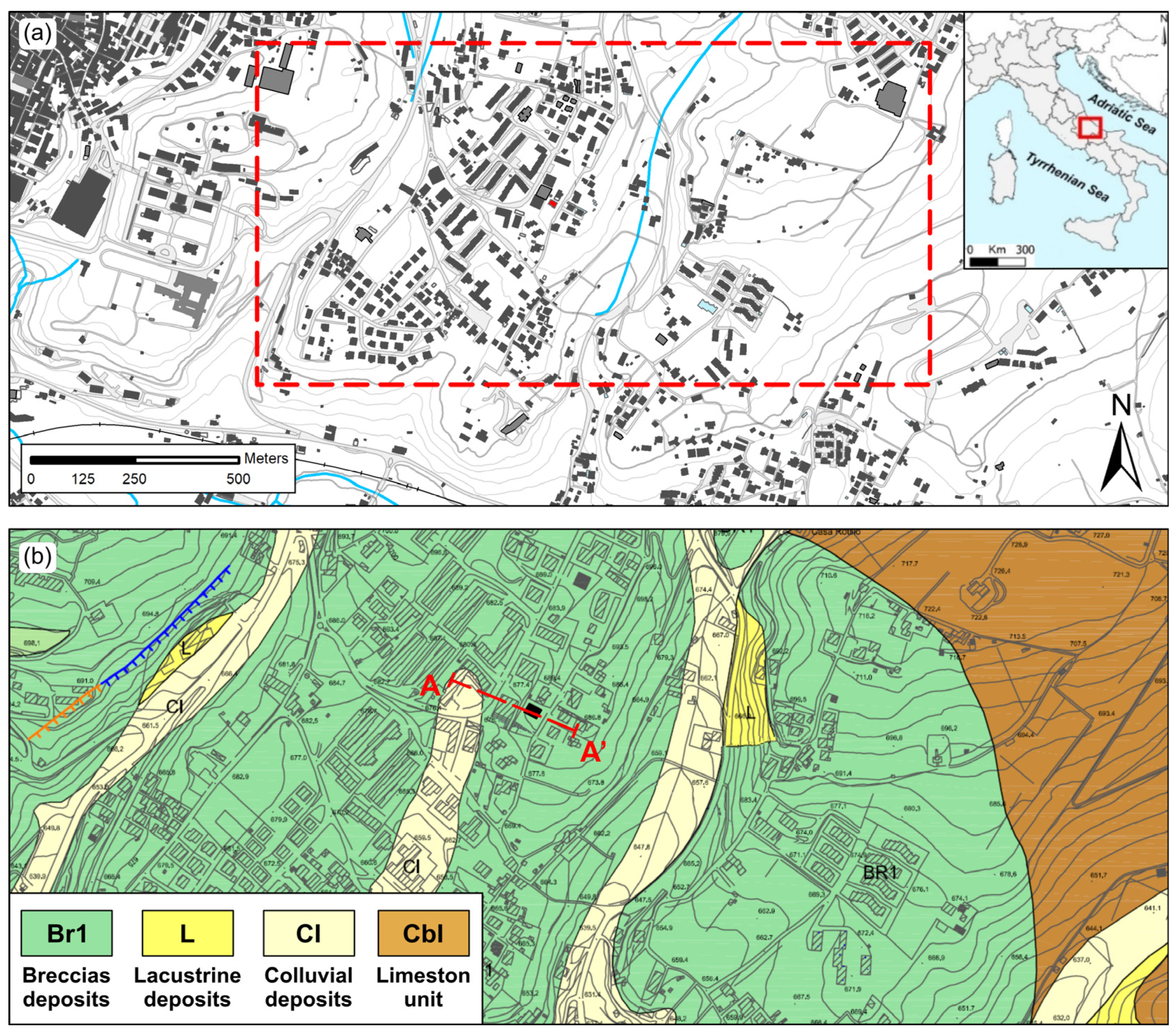
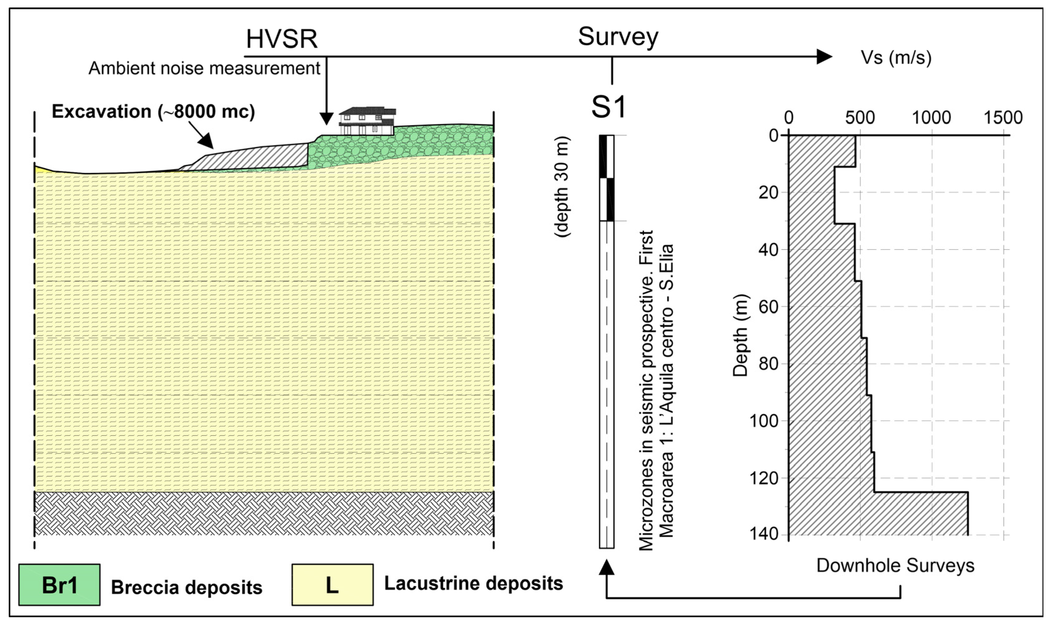
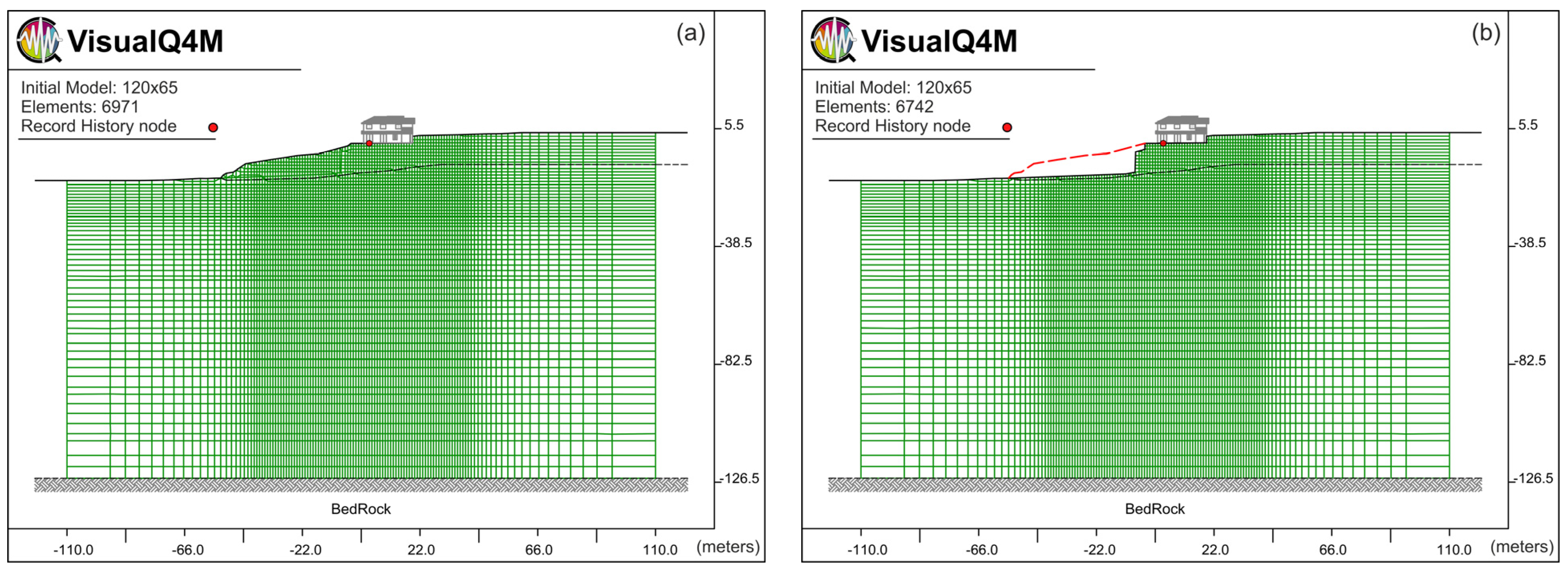
For the test case, a site located in the city of L’Aquila (Italy) was selected [15]. The actual topographic shape is the result of the anthropic excavation realized at the beginning of the 2000s. The natural geometry was modified to realize a private construction in the valley area. About 8000 m³ of soil was removed for the new project, and a prefabricated retaining wall with a height of about 7.50 m was realized. After the main earthquake of April 2009, the upstream structure has been completely damaged. In addition to the classic X-shaped pattern cracks (typical of the seismic action), other types of fissures also appeared, resulting from a sliding movement and minimal vertical deformation of the building. The reduced restriction downstream of the structure generated a relaxation of the horizontal stress component and an increase in the horizontal surface accelerations by topographical amplification. In this case, the simplified approach (1D model) [16] was not correct to simulate multiple reflections of seismic waves on the surface. Thus, 2D simulations were correctly selected.

Moreover, only the fundamental frequencies of the ground have been considered and not those of the structures. Moreover, it should be noted that the Monte Carlo approach, based on the generation of random numbers for the determination of shear wave velocity, introduces frequencies that are not included in the natural frequencies of the selected site [17]. Accordingly, not all seismic frequencies coming from the Fourier analyses of the seismic spectrum, selected as featuring the large scale territory within which is located the particular site under study, could impact the small scale of the site under consideration.

Accordingly, many (pseudo) random, parametric numerical analyses were performed to simulate the seismic wave propagations. In addition, an approach of this type was also useful to understand the impact of a modification of the topography on local seismic analysis after an excavation, including uncertainties considerations as well. Another useful result, based on the statistical standard deviation variability, was the experimental numerical test of how many Monte Carlo simulations were necessary to be performed.

2. Materials and Methods

2.1. Implementation of Pseudo-Random Algorithm

The uncertainties on the assumption of a single and deterministic selection of the numerical values of the shear wave velocity can generate seismic responses that are not always representative of the real site amplifications. Only a probabilistic approach could furnish a more realistic response estimate.

Since the values of the parameters are affected by uncertainty, first of all, through laboratory tests and on-site investigations, a range of variation should be estimated.

For the sake of simplicity, we selected $V_s$ as the primary pseudo-random variable from which to deduce the other ones. In a more general approach, many pseudo-random variables should be considered, requiring, however, a complex cross-correlation analysis and more. Accordingly, the following variability range was estimated:

$$V_{s_{min}}\le V_{s_{RND}}\le V_{s_{max}}$$

(1)

where $V_{s_{RND}}$ = random value; $V_{s_{min}}$ = min value; and $V_{s_{max}}$ = max value were estimated by laboratory and in situ measurements or from the available bibliography (as detailed below). Then, the best estimate of the most probable value (expectation value of the random parameter), i.e., the arithmetic mean between the minimum and maximum value, was introduced:

$${\mu }_{V_s}=\frac{V_{s_{min}}+V_{s_{max}}}{2}$$

(2)

Another important statistical parameter was the “standard deviation” that, following the adopted approach, had to be deduced from the available data. We estimated this parameter on the basis of the well-known “Chebyshev inequality”, according to which about 93% of the numerical value of a random parameter, in our case $V_{s_{RND}}$, lies in the following range [18,19,20,21,22]:

$${\mu }_{V_s}-4{\sigma }_{V_s}\le V_{s_{RND}}\le {\mu }_{V_s}+4{\sigma }_{V_s}$$

(3)

imposing that ${\mu }_{V_s}-4{\sigma }_{V_s}\equiv V_{s_{min}}$ and ${\mu }_{V_s}+4{\sigma }_{V_s}\equiv V_{s_{max}}$, the following important and necessary relation was obtained:

$${\sigma }_{V_s}=\frac{V_{s_{max}}-V_{s_{min}}}{8}$$

(4)

It is worth noting that these assumptions hold independently of the assumed probability distribution to which the random variable belongs.

At this point, we had to define an algebraic expression of a pseudo-random variable, assumed suitable for simulating the numerical values of the mechanical parameters under consideration. The most common approach refers to the following mathematical statement:

$$X_{RND}={\mu }_x+{\sigma }_x\epsilon$$

(5)

where $X_{RND}$ was the pseudo-random parameter, ${\mu }_x$ the average of the total ensemble of numerical values of the $X_{RND}$ parameter (in our case $V_s$), ${\sigma }_x$ the standard deviation around the mean of the selected statistical distribution, while $\epsilon$ was the numerical perturbation due to the uncertainties of the system. We assumed that all the probable and, therefore, real numerical values of the shear velocity are distributed around a mean ${\mu }_x$, with a Normal Gaussian Distribution, among many other possible selections. However, this type of distribution may generate negative values in the tails part of the distribution, which does not make any sense from a geotechnical point of view. Therefore, the algorithm that we implemented includes a requirement that, in case a non-physically consistent value of the random parameter is obtained (for example, a negative value), a value equal to the mean of the assumed statistical ensemble would be assigned to the covering element in consideration. Different statistical distributions will be explored in the future [23]. Accordingly, expression (5) assumed the following expression, specific for the $V_{s_{RND}}$ variable:

$$V_{s_{RND}}={\mu }_{V_s}+{\sigma }_{V_s}·G\_norm$$

(6)

$G\_norm$ was the Normal Gaussian ensemble (a Standard Gaussian Distribution whose mean $\mu$ and standard deviation $\sigma$ are, respectively, 0 and 1):

$$G\_norm=\frac{e^{-\frac{U_{RND}^2}{2}}}{\sqrt{2\pi }}$$

(7)

while $U_{RND}$ was a pseudo-random number.

The C # compiler (very similar to C++), selected in this paper to develop this kind of algorithm, generates, by default, an almost uniform distribution of pseudo-random numbers within a definite range. From this, by means of simple algorithms, it is possible to construct suitable statistical distributions. Accordingly, in order to obtain the distribution (6), the following [24] was selected:

$$G\_norm=\sqrt{-2·\ln \left(U_{rand1}\right)}·\sin \left(2\pi U_{rand2}\right)$$

(8)

The $U_{rand1}$ and $U_{rand2}$ values were two non-correlated (pseudo) random variables uniformly distributed in the interval (0–1). In the resulting distribution, there must be no correlation between $U_{rand1}$ and $U_{rand2}$ variables.

Among other techniques, the Monte Carlo approach [21] was applied, repeating the same calculations several times but considering, for each simulation, different numerical values of the involved parameters belonging to the ensemble described previously.

Through the following expression, the shear modulus was calculated according to the previous discussion:

$$G_{RND}=\rho ·{\left(V_{s_{RND}}\right)}^2$$

(9)

where $G_{RND}$ was the pseudo-random shear modulus; $\rho$ the density (not considered as a random value for the sake of simplicity, but still different for different materials); $V_{s_{RND}}$ the pseudo-random shear wave velocity. Figure 1 shows an example of the outcomes resulting from the application of the method. The shear modulus values were calculated following the Gaussian scheme.

2.2. Computational Tools

The Quad4M software is a 2D Finite Element Method (FEM) code [25]. The grid elements were assembled according to concentrate mass scheme using springs and viscous dampers as connections. The numerical solution is iterative, using a direct integration in the time domain, according to Hughes’s scheme [26]. The calculation procedure uses a system of equations in matrix form [27]:

$$\left[M\right]\ddot{u}+\left[C\right]\dot{u}+\left[K\right]u=R$$

(10)

where:

• [$M]$ = mass matrix (lumped mass formulation);
• [C] = damping matrix;
• [K] = stiffness matrix;
• R = load vector, which is given by: R = [M]${\ddot{u}}_{\mathrm{g}}$;
• ${\dot{u}}_{\mathrm{g}}$ = input velocity;
• ${\ddot{u}}_{\mathrm{g}}$ = input acceleration.

The difficulty in the construction of the conceptual numerical model led to the development of a robust pre- and post-processor capable of simplifying and speeding up the generation of the model and the interpretation of results. The VisualQ4M software includes a graphical user interface (GUI) with functionality and visual command able to generate, with excellent accuracy, geometric models suitable to Quad4M program. Figure 2 shows the flowchart of the VisualQ4M. It is worth noting the set of possibilities, such as the Monte Carlo Method, that were included in this version. The option is valid for Unit Weight, Poisson ratio, shear modulus, and damping ratio, where it is possible to define the variation range for each material according to statistical distributions.

2.3. Geological Model

The site is part of the central Apennine Mountains in a heavily tectonized area (Figure 3). There are soils belonging to the Meso-Cenozoic succession, mainly represented by calcarenite, marly limestone, and bioclastic calcirudite. In the area, these deposits are mostly covered by fluvial deposits, mainly sandy gravel, sandy pelitic lake deposits, and, sometimes, by debris flow and colluvial debris layers. The covering deposits are granular clastic sediments (lake silts, alluvial deposits, debris flow, and pluvio-colluvial deposits). The definition of the geometrical structure and the properties of the layer was carried out by survey report and from the official Geological Map. The local stratigraphy (Figure 4) is composed of an upper seismic layer (carryover terrains and calcareous breccias) and a lower seismic layer of clayey silt materials.

The thickness of the upper layer is about 11.0 m, and the range of the shear wave velocity $V_s$is 391 ± 466 m/s. Silty clay and clayey silt layers (maps of the homogeneous microzones from seismic perspective. First level-Macroarea 1 L’Aquila Centro-S. Elia) are located from 11.0 to 125.0 m; however, direct measurements of their velocities were not available.

$$V_s=300·{\sigma }_m^{\prime }{}^{0.27}-2.44·PI$$

(11)

The $V_s$ profile was estimated by the experimental stresses function by [28], where ${\sigma }_m^{\prime }$ = main effective stress (atm) and $PI$ = plasticity index (15%). The other parameters, density and Poisson ratio (

Table 1. Seismic parameters of the layers.

Lithology	Depth	Density (kN/m3)	Vs (m/s)	Poisson
Calcareous Breccia	0.0–11.0	20.0	433	0.45
Lacustrine deposit	11.0–31.0	19.0	320	0.47
	31.0–51.0	19.0	461	0.47
	51.0–71.0	19.0	507	0.47
	71.0–91.0	19.0	545	0.47
	91.0–111.0	19.0	577	0.47
	111.0–125.0	19.0	597	0.47
Bedrock	125.0–?	22.0	1250	0.30

), were estimated from bibliographic values [29]. Table 1 shows the main parameters used in the analyses.

For the numerical analyses, an equivalent linear model was used [30]. The scarcity of seismic laboratory tests and the impossibility of obtaining undisturbed soil samples in the calcareous breccia led to the use of experimental normalized stiffness G/G₀ and damping ratio, both versus shear strain γ curves, proposed by the study of seismic micro-zonation for the reconstruction of the L’Aquila area. Two stress functions were used, one for the calcareous breccia and another for the lacustrine deposit. The values used for the shear modulus and the damping ratio soil layer are reported in

Table 2. Shear modulus reduction and damping ratio curve for the calcareous breccia.

γ	0.0001	0.001	0.01	0.10	1.00	10.0
G/G0	1.00	0.95	0.75	0.35	0.15	0.15
D	1.00	1.45	3.75	10.55	15.75	16.95

and

Table 3. Shear modulus reduction and damping ratio curve for the lacustrine deposit.

γ	0.0001	0.001	0.01	0.10	1.00	10.0
G/G0	1.00	1.00	0.85	0.25	0.10	0.10
D	3.15	3.30	3.75	10.95	15.95	16.95

.

The effective shear strain for a given soil layer and for a given stress time history was evaluated following Equation (12), where R is the effective strain ratio. In this work, R = 0.65, as suggested in Quad4M manual.

$${\gamma }_{eff}=\mathrm{R}·{\gamma }_{max}$$

(12)

In equivalent-linear analysis, the non-linear response of the soil is approximated by modifying the linear elastic properties of the soil based on the generated strain level. There is no precise rule to determine the max number of the sub-iterations required in Quad4M code, but the VisualQ4M estimate the “Check Run” value. Therefore, the program compares, for each element, the maximum shear strain to the same parameter of the previous run. When there are no more differences, the iteration is stopped.

2.4. Random Variability Model

As discussed by [31], two common methods were used: (1) a single reference $V_s$ profile by varying the values with a constant factor and (2) a statistical approach from random Monte Carlo method. In this work, a combined approach was selected. The Monte Carlo algorithm was implemented with an upper and lower limit selected by $V_s$ average values for each layer, following the previous discussion. The $V_s$ ranges, proposed in Figure 5, were calculated by STRATA code [32]. The code, as described in [33], generates random $V_s$ profiles developed through the procedure proposed by [34].

The algorithm was based on a reference shear-wave profile, and the $V_s$ values were assumed depth-dependent. In this work, a suite of 1000 statistically based random $V_s$ profiles were generated, and the variability range (

Table 4. $V_s$ range used in the numerical analyses.

Depth	Vs (Survey)	Vs (Strata Code)	Range Vs (Strata Code)
(m)	(m/s)	Average (m/s)	Min (m/s)	Max (m/s)
0.0–11.0	433.0	428.2	305.5	550.9
11.0–31.0	320.0	317.4	228.4	406.4
31.0–51.0	461.0	464.3	333.6	595.0
51.0–71.0	507.0	510.2	365.8	654.5
71.0–91.0	545.0	548.7	395.7	701.8
91.0–111.0	577.0	578.0	414.2	741.8
111.0–125.0	597.0	599.7	429.8	769.6

) was successively calculated. In the following table, the “$V_s$(survey)” column shows the $V_s$values recorded in field, while the “V_s (Strata code)” and the “Range V_s (Strata code)” columns show both the Median and the Median ± Log Stdev of $V_s$values calculated by Toro, shown as blue and red lines in Figure 5, respectively [34].

2.5. Geometrical Model

In the numerical modeling, adopting, in particular, the FEM approach, the results also depend on the element size of the grid. Accordingly, numerical tests (not reported) were performed to define an optimal tessellation. The geometric model was calibrated on both the geometric and seismic layers’ characteristics. The grid was assembled through triangular and quadrangular elements with a graded distribution in the horizontal dimension, allowing an effective modeling of geometric variation, as well as irregularities of the topographic surface and stratigraphic contacts. The vertical discretization size directly relates to the accuracy of numerical scheme. The height $h_{max}$ of the element was calculated as follows:

$$h_{max}\le \frac{{\mathsf{\lambda }}_{min}}{10}, {\mathsf{\lambda }}_{min}=\frac{V_s}{f_{max}}$$

(13)

where ${\lambda }_{min}$ was the minimum seismic wavelength of the selected seismic events; $V_s$ was the shear waves velocity; and $f_{max}$ was the maximum frequency (20–25 Hz).

The 2D numerical grids were constructed using the internal discretization algorithm. The code automatically changes both the number of elements and their size in each sub-block to obtain an adaptive gradual elements distribution and, accordingly, a greater numerical precision. Two geometrical models (Figure 6) were analyzed: (A) previous profile shown, reconstructed consulting old maps and previous projects, and (B) the actual profile after excavation, reported and measured through detailed topographic survey.

Both models were implemented with a transmitting boundary at the base so that the need to absorb artificial wave reflections was satisfied [35,36].

2.6. Seismic Input

The seismic simulations were based on actual earthquakes, as they contained realistic frequencies. The accelerograms were selected considering national archives in order to exploit the most representative inputs of the seismicity of the site under examination. The Rexel V.3.5 [37] software was used to extract seven real earthquakes (

Table 5. Seismic Input report.

Event Name	Station Name	Duration (s)	PGA (g)	Moment Magnitude	Epicentral Distance (km)
Emilia_2nd_shock	Mire	61.970	0.173	6.0	4.1
Friuli_3rd_shock	S. Rocco	16.875	0.245	6.0	15.8
L’Aquila	Aquila-V. Aterno	100.000	0.437	6.1	5.0
Central_Italy	Norcia	52.940	0.295	5.4	10.1
Central_italy	Avendita	61.920	0.273	6.5	10.5
Emilia_2nd_shock	Mirandola	63.005	0.213	6.0	5.1
Emilia_2nd_shock	Quarantoli 2	170.005	0.219	6.0	8.6

) whose average matches the target spectrum in the specified range of periods (0.15 s–2.0 s).

3. Results

In the following, the results coming from deterministic and random approaches are compared and discussed.

3.1. Deterministic Approach

In the analysis with a deterministic approach, in order to carry out the simulations relating to the topography before and after the excavation, the different values of $V_s$ waves and, consequently, also the shear modules characterizing the different layers were considered constant and equal to their mean values.

Figure 7 shows the numerical results (seven gray curves), virtually measured in the red dot indicated in Figure 6, following the application of the seven accelerograms required by the Italian National Regulations (as detailed below). Figure 8 also shows, colored in red, the average value of the seven simulations.

The maximum amplitude values and the reference period/frequency for the average acceleration spectrum are shown in the following

Table 6. Maximum spectral acceleration of the mean spectrum.

Stage	Sa	Period	Frequency
Before excavation	0.978 g	0.36 s	2.78 Hz
After excavation	1.051 g	0.36 s	2.78 Hz

.

The horizontal amplification factors $F_{HA}$ were calculated as the ratio of the amplification intensity spectral between the surface $AS{I}_S$ and the acceleration spectrum intensity at the rock outcrop $AS{I}_R$, calculated as follows:

$$F_{HA}=AS{I}_S/AS{I}_R$$

(14)

where $ASI$ [38] was the acceleration spectrum intensity calculated as the integral of the acceleration spectrum between the T₁ and T₂ period:

$$ASI={{\displaystyle \int }}_{T1}^{T2}Sa\left(T,5\%\right)dt$$

(15)

while $Sa\left(T,5\%\right)$ was the spectral acceleration function of the period T, assuming a 5% damping value, as commonly used. The values of T₁ and T₂ were estimated from [39,40].

For the mean spectrum, three interval classes of the vibration periods in seconds, (0.1–0.5), (0.4–0.8), and (0.7–1.1), were used (

Table 7. Mean spectrum amplification $F_{HA}$ (before excavation).

T1 (s)	T2 (s)	ASI (g·s)	ASI0 (g·s)	FHA
0.10	0.50	0.3106	0.2290	1.36
0.40	0.80	0.2999	0.1601	1.87
0.70	1.10	0.2296	0.1027	2.24

and

Table 8. Mean spectrum amplification factor $F_{HA}$ (after excavation).

T1 (s)	T2 (s)	ASI (g·s)	ASI0 (g·s)	FHA
0.10	0.50	0.3349	0.2290	1.46
0.40	0.80	0.2964	0.1601	1.85
0.70	1.10	0.2353	0.1027	2.29

).

3.2. Probabilistic Approach

In the analyses with a probabilistic approach, the $V_s$ wave velocity, and consequently, the shear modulus values, were assumed to be variable for each FEM element according to Table 4 (variability range). The Italian Technical Standards for Construction [39] relating to the analysis of surface seismic amplifications require the consideration of at least seven project accelerograms specific to the site under consideration. For each one of the seven identified accelerograms, 25 distinct realizations were performed, and for each analysis, an independent pseudo-random distribution model was generated. Therefore, 175 analyses (25 × 7) were performed for each of the two geometric models (before and after excavation, Figure 9). In

Table 9. Average spectral acceleration.

Stage	Sa	Period	Frequency
Before excavation	0.974 g	0.28 s	3.571 Hz
After excavation	1.096 g	0.24 s	4.167 Hz

, the period and frequency corresponding to the maximum acceleration spectrum are shown.

Table 10. Mean spectrum amplification factor F_HA (before excavation).

T1 (s)	T2 (s)	ASIS	ASIR	FHA
0.10	0.50	0.3370	0.2290	1.47
0.40	0.80	0.3110	0.1601	1.94
0.70	1.10	0.2600	0.1027	2.53

and

Table 11. Mean spectrum amplification factor F_HA (after excavation).

T1 (s)	T2 (s)	ASIS	ASIR	FHA
0.10	0.50	0.3440	0.2290	1.50
0.40	0.80	0.3110	0.1601	1.94
0.70	1.10	0.2740	0.1027	2.67

list F_HA, coming from 175 probabilistic realizations, considering the topographic surface before and after the excavation, respectively.

Subsequently, the Fourier spectrum was calculated (Figure 9). The Fourier spectrum is defined as the square root of the sum of the squares of the real and imaginary parts of F(ω) (ω is the pulsation). This curve is very important because it indicates the frequency to which most of the energy carried by the waves is associated. With reference to the unique selected control point on the ground surface, it is important to report that the topographic shape did not have any sensible influence on the frequency of the max around 0.891 Hz.

The Monte Carlo method provides a set of numerical results that belong to a certain statistic; the more simulations are carried out, the better the statistics are determined. Therefore, in order to verify the acceptability of the approach and to identify a sufficient number of simulations to be carried out, we selected, as a parameter, the variation of the standard deviation of the ensemble emerging from the application of the method versus the number of repeated simulations. Then, we introduced the “Percentage of Variation” of the standard deviation resulting from n simulations, ${\sigma }_n$, compared to the standard deviation resulting from n − 1 simulations, ${\sigma }_{n-1}$:

$$Percentage of variation=\frac{{\sigma }_n-{\sigma }_{n-1}}{{\sigma }_{n-1}}$$

(16)

In Figure 10, the trend of the standard deviation and its Percentage of Variation, related to amplitude, are reported.

The number of realizations calculated (25 for each earthquake) is sufficient to produce good results. After ten realizations, there are already no significant changes in amplitude and frequency in the spectral output.

3.3. Refined Results Based on Ambient Noise Measurements

The Gaussian distribution produces a variation of the physical parameter around its average value according to a predefined deviation. The variability is the most complex aspect to determine because it is a function of material conditions. To understand which of the 175 realizations are the ones that best identify the actual site conditions, the Fourier spectrum frequencies were compared with the first fundamental frequency of the site. The seismic investigations carried out allowed us to characterize the site by defining a predominant frequency of F_o = 0.888 Hz ± 0.198 Hz. The value was calculated with the HVSR technique (Horizontal-to-Vertical Spectral Ratio).

Subsequently, each individual frequency spectrum was compared with this natural frequency. It is evident that some numerical results do not seem to be congruent with the actual site conditions. To simplify the comparison, a dispersion plot of the pair “Frequency-Peak Amplitude” values of all calculated Fourier spectra were constructed. To exclude non-congruent data, a band-pass filter (BPF) was applied with a central frequency equal to the site frequency of 0.888 Hz and a deviation equal to ±0.198 Hz. Figure 11 shows the pairs of inappropriate and appropriate values and the range considered as a reference for the current study. Figure 12 shows, for the current topographic profile, the final average spectrum calculate with a probabilistic approach and with a band-pass filter (BPF) with respect to the natural frequency of the site.

The maximum amplitude values and the reference period (or frequency) of the average acceleration spectrum, both with and without a filter, are reproduced in

Table 12. Maximum spectral acceleration (current situation).

Average Spectrum	SA	Period	Frequency
Results of all realization	1.086 g	0.26 s	3.85 Hz
Results + Band-Pass filter	1.135 g	0.26 s	3.85 Hz

.

For the average spectrum related to the results coming from the band-pass filter, three interval classes of the vibration periods, in seconds (0.1–0.5), (0.4–0.8), and (0.7–1.1), were used (

Table 13. Amplification factor F_HA for average spectrum results.

T1 (s)	T2 (s)	ASI (g∙s)	ASI0 (g∙s)	FHA
0.10	0.50	0.3300	0.2080	1.60
0.40	0.80	0.2920	0.1420	2.05
0.70	1.10	0.2790	0.0990	2.83

).

The colored maps, shown in Figure 13, display the average values of the max acceleration resulting from some successive realizations labeled by their progressive execution position (the first, the third, etc.). However, in order to compare each realization with the others, the same input motion was considered. The maps are related to the geometry of the system after excavation.

4. Discussion and Conclusions

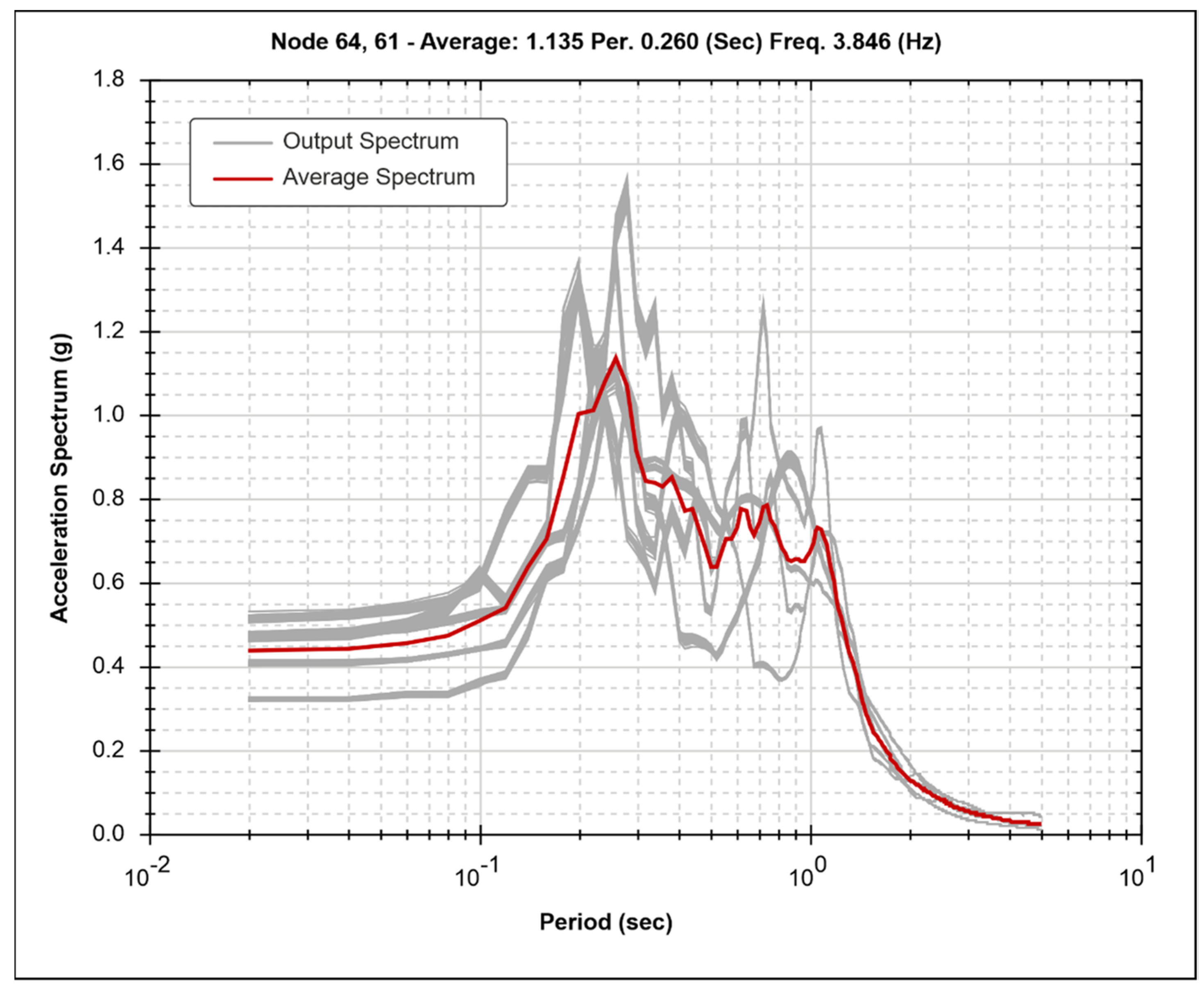
In this paper, the dynamic characterization of the seismic response analysis was based on the shear wave profile. The uncertainties in the definition of the shear wave velocity can generate seismic responses with results that may not be representative of the surface amplifications. Thus, in order to estimate a reasonable seismic response, despite the uncertainties, the Monte Carlo approach was selected. The outcomes of this kind of method were pseudo-random distributions of numerical values according to variability intervals. Sequences of pseudo-random distributions with two geometric configurations were calculated. For each realization of the system under consideration, seven natural waveforms were considered, and for each of them, 25 distinct simulations were performed. The spectrum response was calculated as the average of all 175 resulting spectra. The analysis was carried out according to the equivalent linear model. 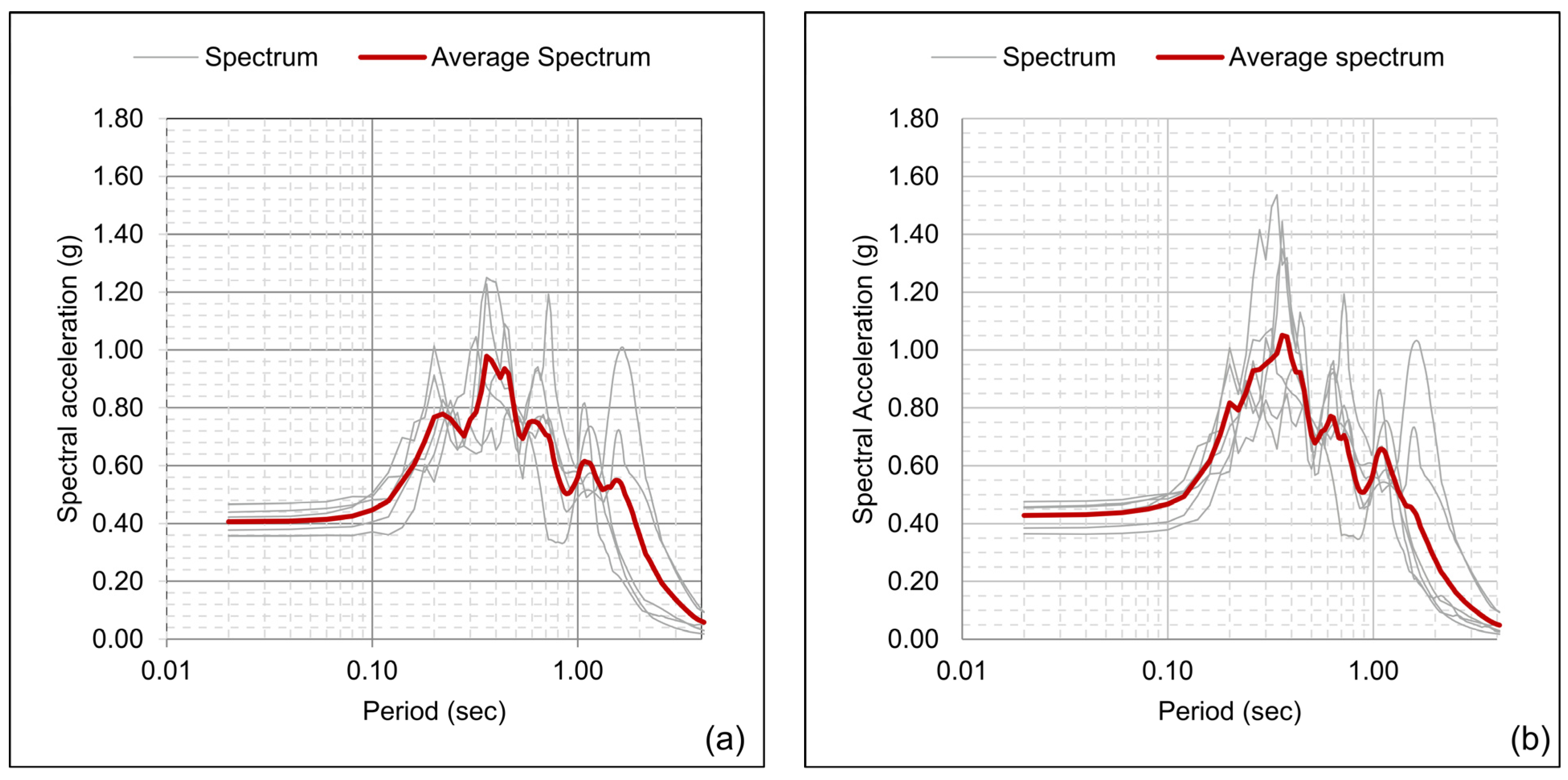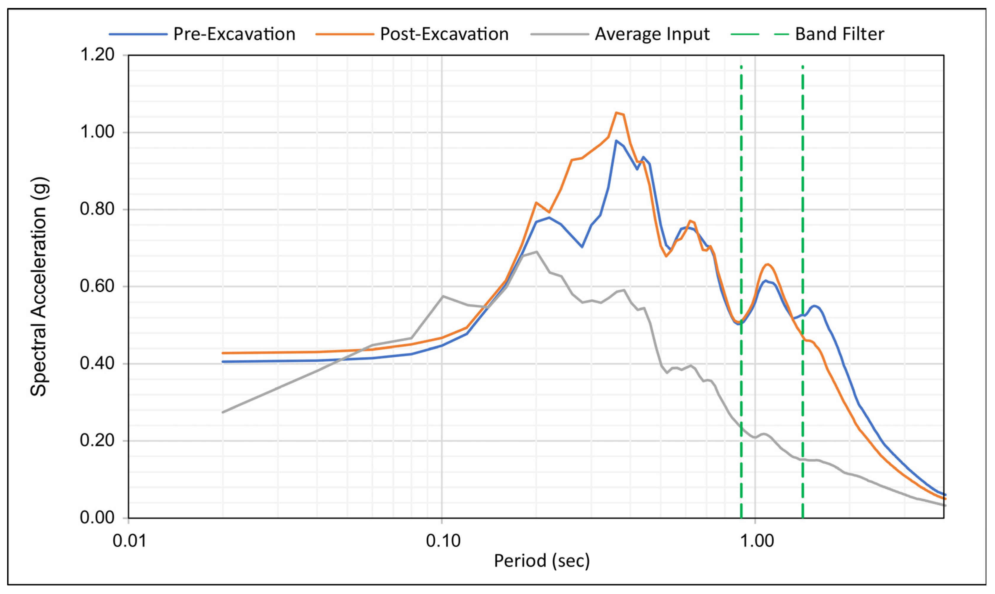The calculations were performed with two distinct approaches: deterministic, for which a unique initial $V_s$ wave velocity was considered for each layer, and probabilistic, for which the $V_s$ wave velocity was calculated as a pseudo-random variable for each element. In the last case, the pseudo-random distribution model was re-calculated at each simulation. Subsequently, only for the probabilistic approach with the actual geometrical profile, the results were compared with the seismic site surveys to select only the realizations compatible with the real conditions. This kind of selection was performed through a band-pass filter (BPF) focused on the fundamental frequency of the site. Comparing the results of the two geometries with the deterministic approach, it is evident that the impact of the topographic modification was important. In fact, from Table 6, it can be observed that the inclusion of the excavation in the numerical simulations caused an increase in the maximum spectral acceleration, raising it from 0.978 g to 1.051, 7% higher, as also displayed in Figure 14, while the period, 0.36 s, was not affected. This aspect is more marked in the higher frequencies.

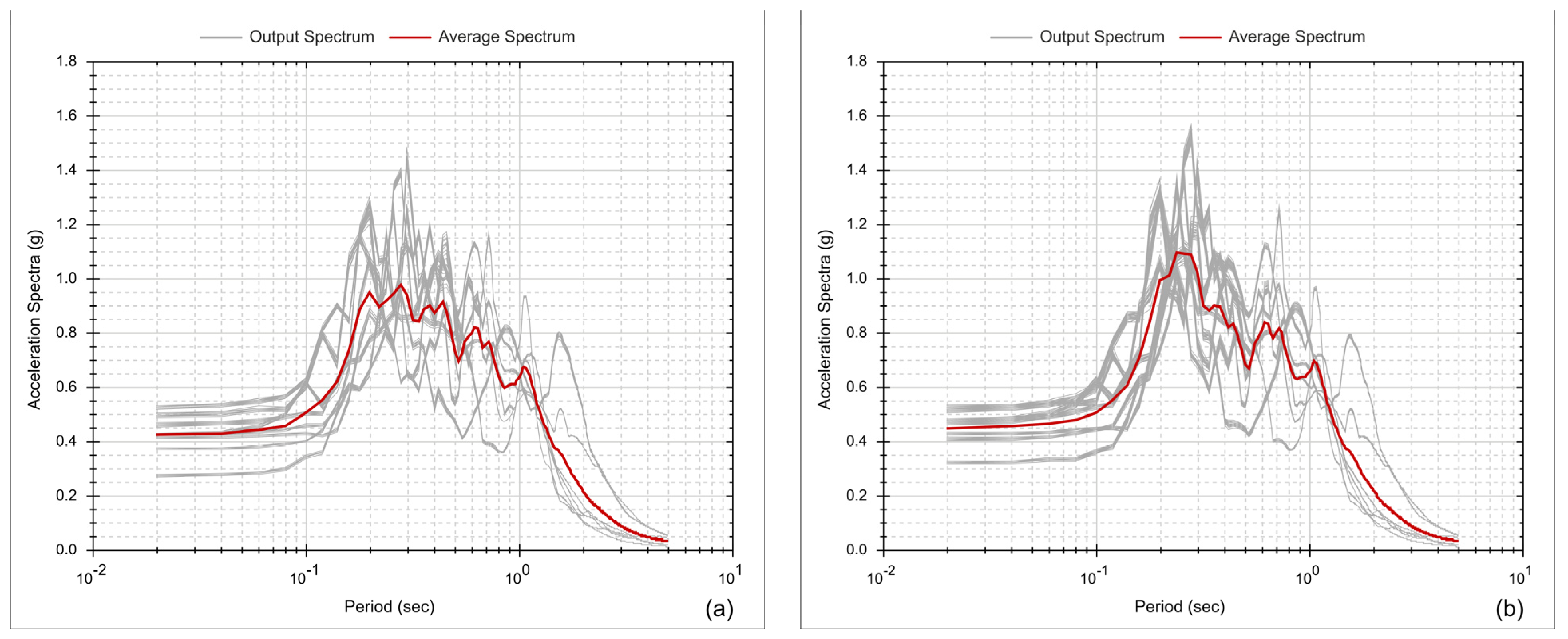
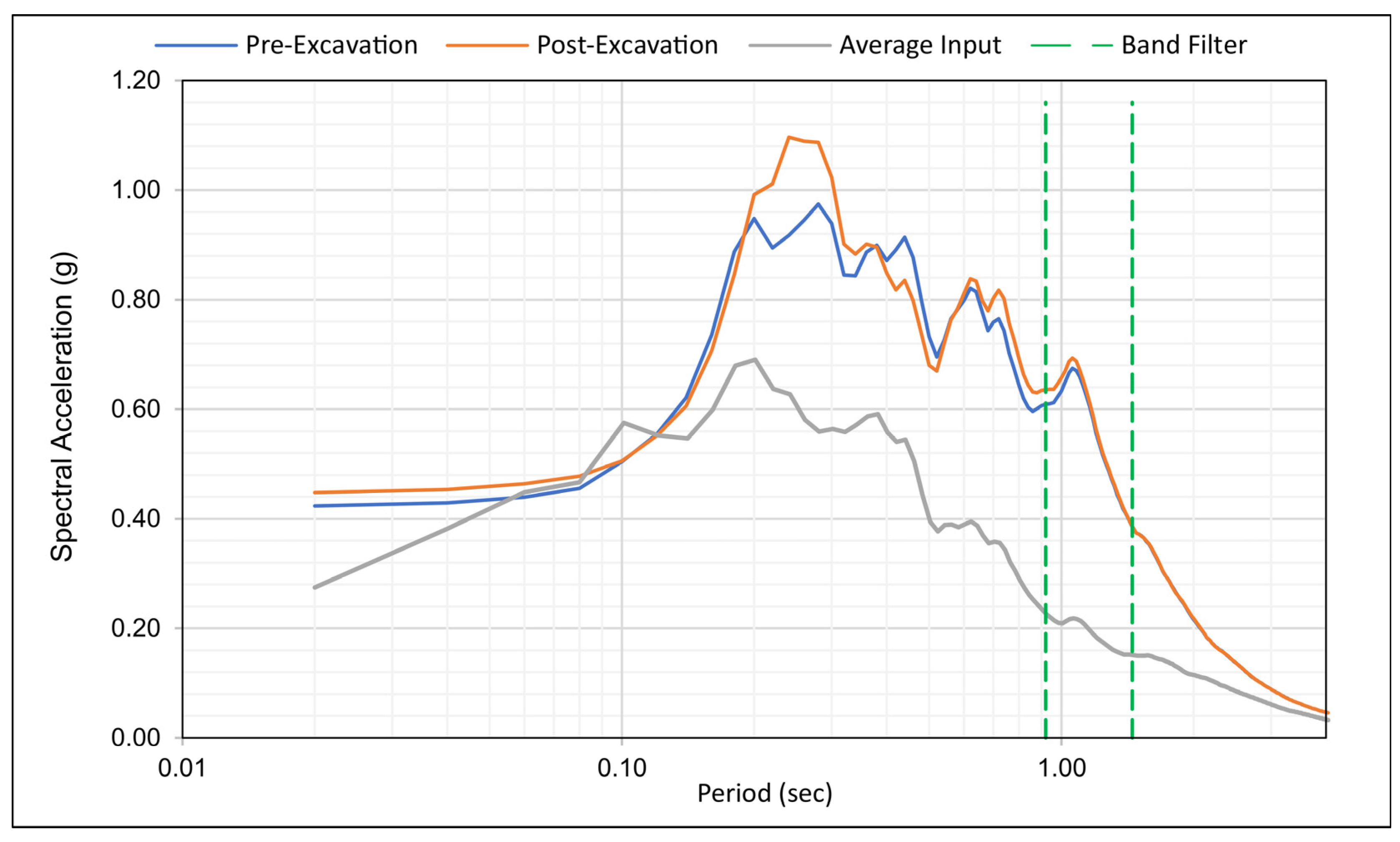
The topographic impact is more evident in the models analyzed with a probabilistic approach. The outcomes of the model, resulting from the inclusion of pseudo-random distribution parameters (shear wave) and the selection of the seven reference accelerograms), show, as can be observed from Table 9 and also from Figure 15, an increase in the maximum spectral acceleration from 0.974 g before excavation to 1.096 after excavation, or 12.5% higher. 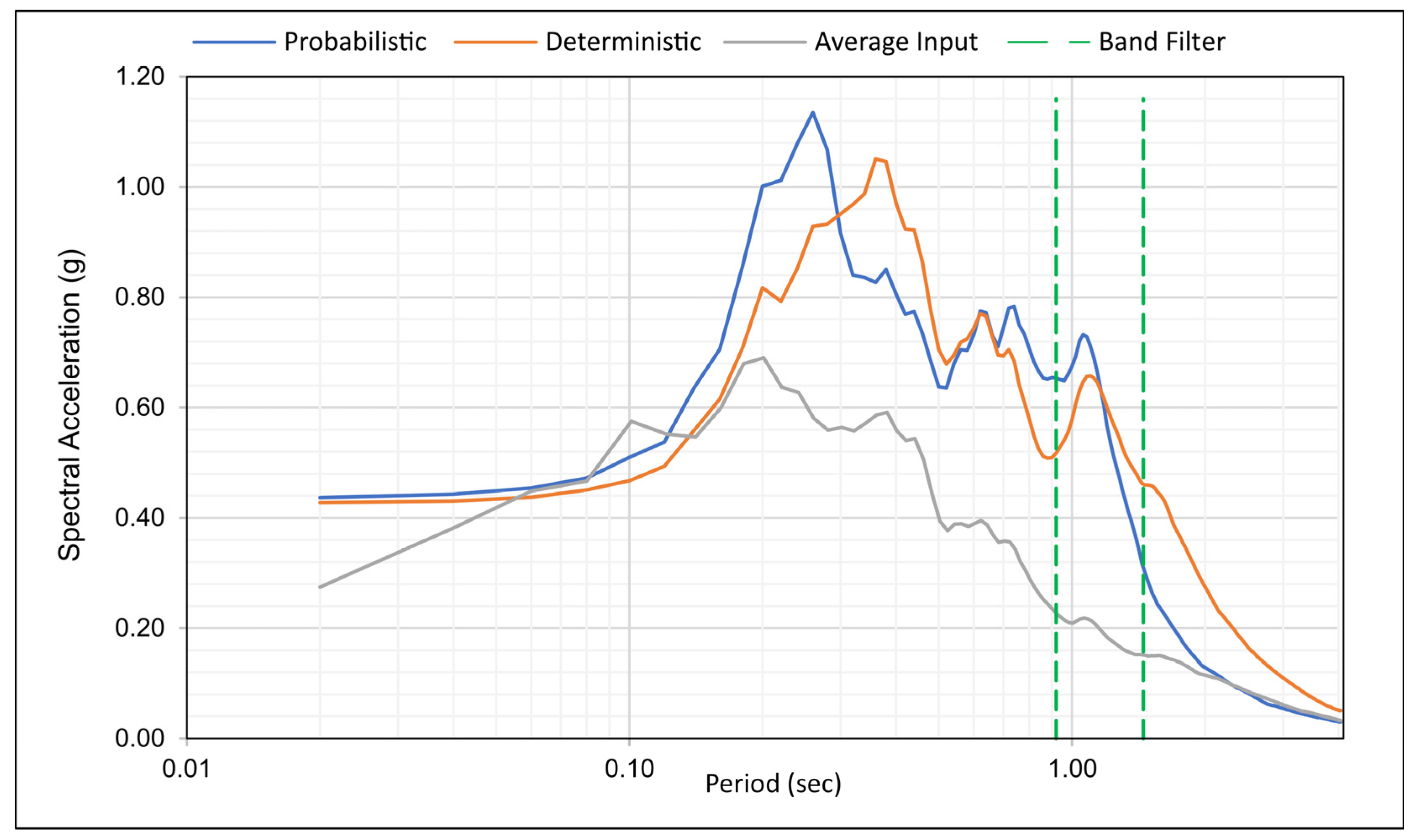Unlike the deterministic case, with the probabilistic approach, the period related to the max value of the acceleration spectrum also changes, decreasing from 0.28 s to 0.24s, 14.4% lower (Table 9). Accordingly, the numerical simulations carried out with the probabilistic approach show a period decrease compared to the values obtained with the deterministic approach of 22.2% and 33.3% pre-excavation and post-excavation, respectively. In order to highlight further important differences emerging from the choice of the methodological approach, Figure 16 displays the comparison between the numerical outcomes resulting from the simulations based on probabilistic and deterministic approaches, both related to the geometry after excavation and the application of the band-pass filter (BPF) centered on the fundamental frequency of the site.

The models based on pseudo-random distributions generated responses with greater values of the amplification factors.

Of course, these differences are also a function of the amount of available data, the laboratory tests, and mainly the quality of the site investigations. Furthermore, in this work, only the $V_s$ (and therefore only the variability of the shear modulus) was considered as a reference parameter, but the surface seismic response could also be a function of the variability influence of other reference parameters or a combination of the same. Using numerical analyses with a pseudo-random approach certainly allows the reduction in the impact due to uncertainties on the determination of seismic parameters and, accordingly, on the estimation of as realistic as possible surface seismic amplification. Moreover, it is believed that not all pseudo-random combinations are representative of the site (especially if a variability on several parameters is used). The comparison with the field survey data (direct and/or indirect tests) is, however, fundamental for the validation of the numerical results.

References

1. Sanò, T.; Pugliese, A. Parametric study on topographic effects in seismic soil amplification. In Proceedings of the Second International Symposium on Earthquake Resistant Engineering Structure, ERES 99, Catania, Italy, 17 June 1999. [Google Scholar]
2. Fabozzi, S.; Catalano, S.; Falcone, G.; Naso, G.; Pagliaroli, A.; Peronace, E.; Porchia, A.; Romagnoli, G.; Moscatelli, M. Stochastic approach to study the site response in presence of shear wave velocity inversion: Application to seismic microzonation studies in Italy. Eng. Geol. 2020, 280, 105914. [Google Scholar] [CrossRef]
3. Kramer, S.L. Geotechnical Earthquake Engineering; Prentice Hall, Inc.: Upper Saddle River, NJ, USA, 1996; p. 653. [Google Scholar]
4. Barani, S.; Ferretti, G.; DeFerrari, R. Incorporating results from seismic microzonation into probabilistic seismic hazard analysis: An example in western Liguria (Italy). Eng. Geol. 2020, 267, 105479. [Google Scholar] [CrossRef]
5. Griffiths, S.C.; Cox, B.R.; Rathje, E.M.; Teague, D.P. Mapping dispersion misfit and uncertainty in Vs profiles to variability in site response estimates. J. Geotech. Geoenviron. Eng. 2016, 142, 04016062. [Google Scholar] [CrossRef]
6. Gobbi, S.; Lenti, L.; Santisi d’Avila, M.P.; Semblat, J.F.; Reiffsteck, P. Influence of the variability of soil profile properties on weak and strong seismic response. Soil Dyn. Earthq. Eng. 2020, 135, 106200. [Google Scholar] [CrossRef]
7. Guzel, Y.; Rouainia, M.; Elia, G. Effect of soil variability on non-linear site response predictions: Application to the Lotung site. Comput. Geotech. 2020, 121, 103444. [Google Scholar] [CrossRef]
8. Seed, H.B.; Idriss, I.M. Influence of soil conditions on ground motions during earthquakes. ASCE J. Soil Mech. Found Div. 1969, 99, 137. [Google Scholar] [CrossRef]
9. Ghanem, R.G.; Spanos, P.D. Stochastic Finite Elements—A Spectral Approach; Dover Publications Inc.: Mineola, NY, USA, 1991; ISBN 0-486-42818-4. [Google Scholar]
10. Hudson, M.; Idriss, I.M.; Beikae, M. QUAD4M: A Computer Program to Evaluate the Seismic Response of Soil Structures Using Finite Element Procedures and Incorporating a Compliant Base; Center for Geotechnical Modeling, Department of Civil and Environmental Engineering, University of California Davis: Davis, CA, USA, 1994. [Google Scholar]
11. Mangifesta, M. VisualQ4M. Pre & Post Processor for the Evaluation of the Seismic Response. 2021. Available online: http://www.visualq4m.com (accessed on 16 January 2013).
12. Hastings, W.K. Monte Carlo Sampling Methods Using Markov Chains and Their Applications. Biometrika 1970, 57, 97–109. [Google Scholar] [CrossRef]
13. Jesse Burgess, G.; Fenton, A.; Griffiths, D.V. Probabilistic seismic slope stability analysis and design. Can. Geotech. J. 2019, 56, 1979–1998. [Google Scholar] [CrossRef] [Green Version]
14. Li, Y.; Zhang, F.; Yeh, T.-C.J.; Hou, X.; Dong, M. Cross-Correlation Analysis of the Stability of Heterogeneous Slopes. Water 2023, 15, 1050. [Google Scholar] [CrossRef]
15. Carta Geologica. Progetto Microzonazione Sismica L’Aquila: Macroarea 1 (L’Aquila, Italy). May–December 2009, Editor Dipartimento di Ingegneria delle Strutture, delle Acque e del Terreno, Università dell’Aquila e Dipartimento di Protezione Civile Nazionale. (In Italian)
16. Özcebe, A.G.; Smerzini, C.; Paolucci, R.; Pourshayegan, H.; Rodríguez Plata, R.; Lai, C.G.; Zuccolo, E.; Bozzoni, F.; Villani, M. On the comparison of 3D, 2D, and 1D numerical approaches to predict seismic site amplification: The case of Norcia basin during the M6. 5 2016 October 30 earthquake. In Proceedings of the 7th International Conference on Earthquake Geotechnical Engineering, Roma, Italy, 16–20 June 2019; pp. 4251–4258. [Google Scholar]
17. Mori, F.; Gaudiosi, I.; Tarquini, E.; Bramerini, F.; Castenetto, S.; Naso, G.; Spina, D. HSM: A synthetic damage-constrained seismic hazard parameter. Bull. Earthq. Eng. 2020, 18, 5631–5654. [Google Scholar] [CrossRef]
18. Pasculli, A.; Calista, M.; Mangifesta, M. The effects of spatial variability of mechanical parameters on a 3D landslide study. In Proceedings of the 4th International FLAC Symposium, Madrid, Spain, 29–31 May 2006; ISBN 0-9767577-0-2. [Google Scholar]
19. Pasculli, A.; Pugliese, A.; Romeo, R.W.; Sanò, T. The uncertainty in the Local Seismic Response Analysis. In Proceedings of the 2008 Seismic Engineering International Conference MERCEA 08 AIP (American Institute of Physics), Messina, Italy, 8–11 July 2008; Volume 1020, pp. 321–328. [Google Scholar]
20. Calista, M.; Pasculli, A.; Sciarra, N. Reconstruction of the geotechnical model considering random parameters distributions. Eng. Geol. Soc. Territ. 2015, 2, 1347–1351. [Google Scholar] [CrossRef]
21. Pasculli, A.; Calista, M.; Sciarra, N. Variability of local stress states resulting from the application of Monte Carlo and finite difference methods to the stability study of a selected slope. Eng. Geol. 2018, 245, 370–389. [Google Scholar] [CrossRef]
22. Pasculli, A.; Mangifesta, M. Local seismic response change following an excavation in an area located in the territory of L’Aquila City (Italy). In Proceedings of the International Conference of Numerical Analysis and Applied Mathematics ICNAAM, Rhodes, Greece, 23–28 September 2019; Volume 2293, pp. 420072-1–420072-6. [Google Scholar] [CrossRef]
23. Uzielli, M.; Lacasse, S.; Nadim, F.; Phoon, K.K. Soil variability analysis for geotechnical practice. Characterisation Eng. Prop. Nat. Soils 2007, 3–4, 1653–1752. [Google Scholar]
24. Box, G.E.P.; Muller, M.E. A note on generation of random normal deviates. Ann. Math. Stat. 1958, 29, 610–611. [Google Scholar] [CrossRef]
25. Idriss, I.M.; Lysmer, J.; Hwang, R.; Seed, H.B. QUAD-4. A Computer Program for Evaluating the Seismic Response of Soil Structures by Variable Damping; Finite Element Procedures, Earthquake Engineering Research Center, Report N. EERC 73-16; University of California: Berkeley, CA, USA, 1973. [Google Scholar]
26. Hughes, T.J.R. The Finite Element Method; Prentice Hall: London, UK, 1987. [Google Scholar]
27. Newmark, N.M. A method of computation for structural dynamics. J. Eng. Mech. ASCE 1959, 85, 67–94. [Google Scholar] [CrossRef]
28. Chiara, N. Investigation of Small-Strain Shear Stiffness Measured in Field and Laboratory Geotechnical Studies. Master’s Thesis, University of Texas at Austin, Austin, TX, USA, 2001. [Google Scholar]
29. Di Capua, G.; Lanzo, G.; Luzi, L.; Pacor, F.; Paolucci, R.; Peppoloni, S.; Scasserra, G.; Puglia, R. Caratteristiche geologiche e classificazione di sito delle stazioni accelerometriche della RAN ubicate a L’Aquila. In Rapporto Progetto S4: Banca Dati Accelerometrica Giugno; 2009; p. 28. Available online: http://esse4.mi.ingv.it (accessed on 16 January 2023). (In Italian)
30. Kuhlemeyer, R.L.; Lysmer, J. Finite element method accuracy for wave propagation problems. J. Soil Mech. Found. Div. 1973, 5, 421–427. [Google Scholar] [CrossRef]
31. Cox, S.C.; Griffiths, E.M.; Rathje, D.; Teague, P. Shear Wave Velocity Uncertainty and Its Relation to Variability in Site Response Using a Dispersion Misfit Approach. International Society for Soil Mechanics and Geotechnical Engineering. In Proceedings of the 6th International Conference on Earthquake Geotechnical Engineering, Christchurch, New Zealand, 1–4 November 2015. [Google Scholar]
32. Kottke, A.; Rathje, E. Technical Manual for Strata; Report No. 2008/10; Pacific Earthquake Engineering Research Center: Berkeley, CA, USA, 2013. [Google Scholar]
33. Rathje, E.M.; Kottke, A.R.; Trent, W.L. Influence of Input Motion and Site Property Variabilities on Seismic Site Response Analysis. J. Geotech. Geoenviron. Eng. 2010, 136, 607–619. [Google Scholar] [CrossRef]
34. Toro, G. Probabilistic Models of the Site Velocity Profiles for Generic and Site Specific Ground Motion Amplification Studies; Technical Report No. 779574; Brookhaven National Laboratory: Upton, NY, USA, 1995; p. 147. [Google Scholar]
35. Chiaradonna, A. Defining the Boundary Conditions for Seismic Response Analysis. A Practical Review of Some Widely-Used Codes. Geosciences 2022, 12, 83. [Google Scholar] [CrossRef]
36. Falcone, G.; Naso, G.; Mori, F.; Mendicelli, A.; Acunzo, G.; Peronace, E.; Moscatelli, M. Effect of Base Conditions in One-Dimensional Numerical Simulation of Seismic Site Response: A Technical Note for Best Practice. GeoHazards 2021, 2, 430–441. [Google Scholar] [CrossRef]
37. Iervolino, I.; Galasso, C.; Cosenza, E. REXEL: Computer aided record selection for code-based seismic structural analysis. Bull. Earthq. Eng. 2010, 8, 2010. [Google Scholar] [CrossRef]
38. Von Thun, J.L.; Rochim, L.H.; Scott, G.A.; Wilson, J.A. Earthquake ground motions for design and analysis of dams. In Earthquake Engineering and Soil Dynamics II—Recent Advances in Ground-Motion Evaluation (GSP 20); ASCE: New York, NY, USA, 1988; pp. 463–481. [Google Scholar]
39. SM Working Group. Guidelines for Seismic Microzonation; English Version; SM Working Group: Rome, Italy, 2015. [Google Scholar]
40. Falcone, G.; Acunzo, G.; Mendicelli, A.; Mori, F.; Naso, G.; Peronace, E.; Porchia, A.; Romagnoli, G.; Tarquini, E.; Moscatelli, M. Seismic amplification maps of Italy based on site-specific microzonation dataset and one-dimensional numerical approach. Eng. Geol. 2021, 289, 106170. [Google Scholar] [CrossRef]
Figure 1. Example of Monte Carlo approach.: (a) Shear modulus distribution with depth; (b) Normal distribution of shear modulus.
Geosciences 13 00165 g001
Figure 2. VisualQ4M flow chart implementation.
Geosciences 13 00165 g002
Figure 3. Test case location in city of L’Aquila (a). Geological map of the urban area of the L’Aquila city -First level-Macroarea 1 (b). The red line is the Section A-A’ used in analyses.
Geosciences 13 00165 g003
Figure 4. Schematic seismic-layer section and survey location.
Geosciences 13 00165 g004
Figure 5. The 1000 V s profiles calculated by (STRATA Code) [34].
Geosciences 13 00165 g005
Figure 6. Meshes of discretization used to analyze the topographic profile. (a) Before excavation. (b) After excavation.
Geosciences 13 00165 g006
Figure 7. Acceleration spectrum in deterministic approach. (a) Before excavation. (b) After excavation.
Geosciences 13 00165 g007
Figure 8. Acceleration spectra in probabilistic approach. (a) Before excavation. (b) After excavation.
Geosciences 13 00165 g008
Figure 9. Average Fourier spectra for the pre- and post-excavation probabilistic case studies.
Geosciences 13 00165 g009
Figure 10. Max standard deviation and percentage of variation in amplitude versus number of realizations.
Geosciences 13 00165 g010
Figure 11. Band-pass filter (BPF) application. This operation excludes all conflicting results.
Geosciences 13 00165 g011
Figure 12. Acceleration spectrum with band-pass filter after excavation.
Geosciences 13 00165 g012
Figure 13. Maximum horizontal acceleration for the after-excavation case study: (a) realization 1; (b) realization 3; (c) realization 5; and (d) realization 10.
Geosciences 13 00165 g013
Figure 14. Comparison between the two different geometries; deterministic approach.
Geosciences 13 00165 g014
Figure 15. Comparison between the two different geometries; probabilistic approach.
Geosciences 13 00165 g015
Figure 16. Comparison between deterministic and probabilistic approach after excavation.
Geosciences 13 00165 g016