

Mathematical Simulation of Honeycomb Weathering via Moisture Transport and Salt Deposition

Abstract
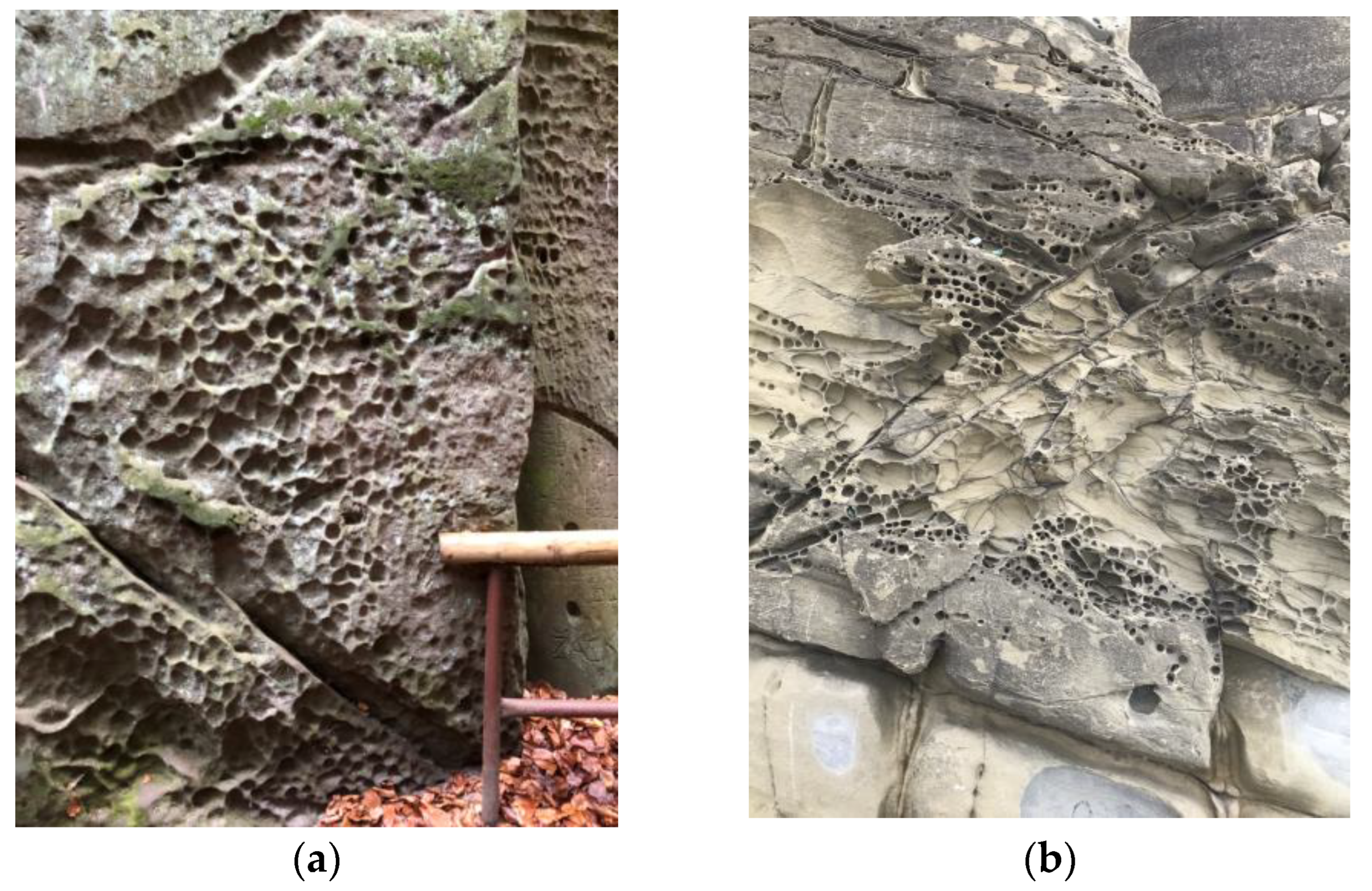
:1. Introduction
2. Methods
3. Results and Discussion
4. Conclusions
Supplementary Materials
Author Contributions
Funding
Data Availability Statement
Acknowledgments
Conflicts of Interest
References
- Smith, P.J. Why honeycomb weathering? Nature 1982, 298, 121–122. [Google Scholar] [CrossRef]
- Mustoe, G.E. The origin of honeycomb weathering. Geol. Soc. Am. Bull. 1982, 93, 108–115. [Google Scholar] [CrossRef]
- Groom, K.M.; Allen, C.D.; Mol, L.; Paradise, T.R.; Hall, K. Defining tafoni: Re-examining terminological ambiguity for cavernous rock decay phenomena. Prog. Phys. Geogr. 2015, 39, 775–793. [Google Scholar] [CrossRef]
- Bruthans, J.; Filippi, M.; Slavík, M.; Svobodová, E. Origin of honeycombs: Testing the hydraulic and case hardening hypotheses. Geomorphology 2018, 303, 68–83. [Google Scholar] [CrossRef]
- Filippi, M.; Bruthans, J.; Řihošek, J.; Slavík, M.; Adamovič, J.; Mašín, D. Arcades: Products of stress-controlled and discontinuity-related weathering. Earth-Sci. Rev. 2018, 180, 159–184. [Google Scholar] [CrossRef]
- Evelpidou, N.; Karkani, A.; Tzouxanioti, M.; Spyrou, E.; Petropoulos, A.; Lakidi, L. Inventory and Assessment of the Geomorphosites in Central Cyclades, Greece: The Case of Paros and Naxos Islands. Geosciences 2021, 11, 512. [Google Scholar] [CrossRef]
- Migoń, P. Sandstone geomorphology—Recent advances. Geomorphology 2021, 373, 107484. [Google Scholar] [CrossRef]
- Mustoe, G.E. Biogenic origin of coastal honeycomb weathering. Earth Surf. Process. Landf. 2010, 35, 424–434. [Google Scholar] [CrossRef]
- McBride, E.F.; Picard, M.D. Origin of honeycombs and related weathering forms in Oligocene Macigno Sandstone, Tuscan coast near Livorno, Italy. Earth Surf. Process. Landf. 2004, 29, 713–735. [Google Scholar] [CrossRef]
- Prebble, M.M. Cavernous weathering in the taylor dry Valley, Victoria Land, Antarctica. Nature 1967, 216, 1194–1195. [Google Scholar] [CrossRef]
- André, M.F.; Hall, K. Honeycomb development on Alexander Island, glacial history of George VI Sound and palaeoclimatic implications (Two Step Cliffs/Mars Oasis, W Antarctica). Geomorphology 2005, 65, 117–138. [Google Scholar] [CrossRef]
- Inkpen, R.; Hall, K. Universal shapes? Analysis of the shape of antarctic tafoni. Geosciences 2019, 9, 154. [Google Scholar] [CrossRef]
- Strini, A.; Guglielmin, M.; Hall, K. Tafoni development in a cryotic environment: An example from Northern Victoria Land, Antarctica. Earth Surf. Process. Landf. 2008, 33, 1502–1519. [Google Scholar] [CrossRef]
- Dragovich, D. Building Stone and Its Use in Rock Weathering Studies. J. Geol. Educ. 1979, 27, 21–25. [Google Scholar] [CrossRef]
- Siedel, H. Alveolar weathering of Cretaceous building sandstones on monuments in Saxony, Germany. Geol. Soc. Spec. Publ. 2010, 333, 11–23. [Google Scholar] [CrossRef]
- Oguchi, C.T.; Yu, S. A review of theoretical salt weathering studies for stone heritage. Prog. Earth Planet. Sci. 2021, 8, 32. [Google Scholar] [CrossRef]
- Pötzl, C.; Siegesmund, S.; Dohrmann, R.; Koning, J.M.; Wedekind, W. Deterioration of volcanic tuff rocks from Armenia: Constraints on salt crystallization and hydric expansion. Environ. Earth Sci. 2018, 77, 660. [Google Scholar] [CrossRef]
- Rodriguez-Navarro, C. Evidence of honeycomb weathering on Mars. Geophys. Res. Lett. 1998, 25, 3249–3252. [Google Scholar] [CrossRef]
- Smith, P.J. Can honeycomb weathering be ET? Nature 1983, 301. [Google Scholar] [CrossRef]
- Schnepfleitner, H.; Sass, O.; Fruhmann, S.; Viles, H.; Goudie, A. A multi-method investigation of temperature, moisture and salt dynamics in tafoni (Tafraoute, Morocco). Earth Surf. Process. Landf. 2016, 41, 473–485. [Google Scholar] [CrossRef]
- Rodriguez-Navarro, C.; Doehne, E.; Sebastian, E. Origins of honeycomb weathering: The role of salts and wind. Bull. Geol. Soc. Am. 1999, 111, 1250–1255. [Google Scholar] [CrossRef]
- Conca, J.L.; Rossman, G.R. Case hardening of sandstone. Geology 1982, 10, 520–523. [Google Scholar] [CrossRef]
- Turkington, A.V.; Paradise, T.R. Sandstone weathering: A century of research and innovation. Geomorphology 2005, 67, 229–253. [Google Scholar] [CrossRef]
- Zwalińska, K.; Dąbski, M. Cavernous weathering forms in SW Iceland: A case study on weathering of basalts in a cold temperate maritime climate. Misc. Geogr. 2012, 16, 11–16. [Google Scholar] [CrossRef]
- Klimchouk, A. Tafoni and honeycomb structures as indicators of ascending fluid flow and hypogene karstification. Geol. Soc. Lond. Spec. Publ. 2018, 466, 79–105. [Google Scholar] [CrossRef]
- Paradise, T.R. Tafoni and Other Rock Basins. In Treatise on Geomorphology; Academic Press: San Diego, CA, USA, 2013; Volume 4. [Google Scholar]
- Viles, H.A. Scale issues in weathering studies. Geomorphology 2001, 41, 63–72. [Google Scholar] [CrossRef]
- Bruthans, J.; Soukup, J.; Vaculikova, J.; Filippi, M.; Schweigstillova, J.; Mayo, A.L.; Masin, D.; Kletetschka, G.; Rihosek, J. Sandstone landforms shaped by negative feedback between stress and erosion. Nat. Geosci. 2014, 7, 597–601. [Google Scholar] [CrossRef]
- Řihošek, J.; Slavík, M.; Bruthans, J.; Filippi, M. Evolution of natural rock arches: A realistic small-scale experiment. Geology 2019, 47, 71–74. [Google Scholar] [CrossRef]
- Ostanin, I.; Safonov, A.; Oseledets, I. Natural Erosion of Sandstone as Shape Optimisation. Sci. Rep. 2017, 7, 17301. [Google Scholar] [CrossRef]
- Moore, J.R.; Geimer, P.R.; Finnegan, R.; Bodtker, J. Between a beam and catenary: Influence of geometry on gravitational stresses and stability of natural rock arches. Geomorphology 2020, 364, 107244. [Google Scholar] [CrossRef]
- Safonov, A.A. Computing via natural erosion of sandstone. Int. J. Parallel Emergent Distrib. Syst. 2018, 33, 742–751. [Google Scholar] [CrossRef]
- Safonov, A.; Filippi, M.; Mašín, D.; Bruthans, J. Numerical modeling of the evolution of arcades and rock pillars. Geomorphology 2020, 365, 107260. [Google Scholar] [CrossRef]
- Huinink, H.P.; Pel, L.; Kopinga, K. Simulating the growth of tafoni. Earth Surf. Process. Landforms 2004, 29, 1225–1233. [Google Scholar] [CrossRef]
- Philip, J.R. The theory of infiltration: 1. The infiltration equation and its solution. Soil Sci. 1957, 83, 345–358. [Google Scholar] [CrossRef]
- Pel, L.; Kopinga, K.; Brocken, H. Moisture transport in porous building materials. Heron 1996, 41, 95–105. [Google Scholar]
- Landman, K.A.; Pel, L.; Kaasschieter, E.F. Analytic modelling of drying of porous materials. Math. Eng. Ind. 2001, 8, 89–122. [Google Scholar] [CrossRef]
- Pel, L.; Landman, K.A. A Sharp Drying Front Model. Dry. Technol. 2004, 22, 637–647. [Google Scholar] [CrossRef]
- Abaqus/CAE, Simulia. Available online: https://www.3ds.com/products-services/simulia/products/abaqus/abaquscae/ (accessed on 25 May 2023).
- Safonov, A.A. 3D topology optimization of continuous fiber-reinforced structures via natural evolution method. Compos. Struct. 2019, 215, 289–297. [Google Scholar] [CrossRef]
- Safonov, A.; Chugunov, S.; Tikhonov, A.; Gusev, M.; Akhatov, I. Numerical simulation of sintering for 3D-printed ceramics via SOVS model. Ceram. Int. 2019, 45, 19027–19035. [Google Scholar] [CrossRef]
- Vedernikov, A.; Safonov, A.; Tucci, F.; Carlone, P.; Akhatov, I. Modeling spring-in of l-shaped structural profiles pultruded at different pulling speeds. Polymers 2021, 13, 2748. [Google Scholar] [CrossRef]
- Safonov, A.; Jones, J. Physarum computing and topology optimisation. Int. J. Parallel Emergent Distrib. Syst. 2017, 32, 448–465. [Google Scholar] [CrossRef]
- Moskaleva, A.; Gusev, S.; Konev, S.; Sergeichev, I.; Safonov, A.; Hernandez-Montes, E. Composite freeform shell structures: Design, construction and testing. Compos. Struct. 2023, 306, 116603. [Google Scholar] [CrossRef]
- Safonov, A.; Adamatzky, A. Computing via material topology optimisation. Appl. Math. Comput. 2018, 318, 109–120. [Google Scholar] [CrossRef]
- Wellman, H.W.; Wilson, A.T. Salt weathering, a neglected geological erosive agent in coastal and arid environments. Nature 1965, 205, 1097–1098. [Google Scholar] [CrossRef]
- Flatt, R.J.; Caruso, F.; Sanchez, A.M.A.; Scherer, G.W. Chemo-mechanics of salt damage in stone. Nat. Commun. 2014, 5, 4823. [Google Scholar] [CrossRef]
- Schiro, M.; Ruiz-Agudo, E.; Rodriguez-Navarro, C. Damage mechanisms of porous materials due to in-pore salt crystallization. Phys. Rev. Lett. 2012, 109, 265503. [Google Scholar] [CrossRef]
- Rijniers, L.A.; Huinink, H.P.; Pel, L.; Kopinga, K. Experimental evidence of crystallization pressure inside porous media. Phys. Rev. Lett. 2005, 94, 075503. [Google Scholar] [CrossRef] [PubMed]
- Flatt, R.J. Salt damage in porous materials: How high supersaturations are generated. J. Cryst. Growth 2002, 242, 435–454. [Google Scholar] [CrossRef]
- Rodriguez-Navarro, C.; Doehne, E. Salt weathering: Influence of evaporation rate, supersaturation and crystallization pattern. Earth Surf. Process. Landf. 1999, 24, 191–209. [Google Scholar] [CrossRef]
- Scherer, G.W. Stress from crystallization of salt. Cem. Concr. Res. 2004, 34, 1613–1624. [Google Scholar] [CrossRef]
- Charola, A.E. Salts in the Deterioration of Porous Materials: An Overview. J. Am. Inst. Conserv. 2000, 39, 327–343. [Google Scholar] [CrossRef]
- D’Altri, A.M.; de Miranda, S.; Beck, K.; De Kock, T.; Derluyn, H. Towards a more effective and reliable salt crystallisation test for porous building materials: Predictive modelling of sodium chloride salt distribution. Constr. Build. Mater. 2021, 304, 124436. [Google Scholar] [CrossRef]
- Gupta, S.; Huinink, H.P.; Prat, M.; Pel, L.; Kopinga, K. Paradoxical drying of a fired-clay brick due to salt crystallization. Chem. Eng. Sci. 2014, 109, 204–211. [Google Scholar] [CrossRef]
- Gonçalves, T.D.; Brito, V.; Pel, L. Water Vapor Emission From Rigid Mesoporous Materials during the Constant Drying Rate Period. Dry. Technol. 2012, 30, 462–474. [Google Scholar] [CrossRef]
- Ketelaars, A.A.J.; Pel, L.; Coumans, W.J.; Kerkhof, P.J.A.M. Drying kinetics: A comparison of diffusion coefficients from moisture concentration profiles and drying curves. Chem. Eng. Sci. 1995, 50, 1187–1191. [Google Scholar] [CrossRef]
- Pel, L.; Pishkari, R.; Casti, M. A simplified model for the combined wicking and evaporation of a NaCl solution in limestone. Mater. Struct. 2018, 51, 66. [Google Scholar] [CrossRef]
- Mareš, J.; Bruthans, J.; Weiss, T.; Filippi, M. Coastal honeycombs (Tuscany, Italy): Moisture distribution, evaporation rate, tensile strength, and origin. Earth Surf. Process. Landf. 2022, 47, 1653–1667. [Google Scholar] [CrossRef]
- Slavík, M.; Bruthans, J.; Weiss, T.; Schweigstillová, J. Measurements and calculations of seasonal evaporation rate from bare sandstone surfaces: Implications for rock weathering. Earth Surf. Process. Landf. 2020, 45, 2965–2981. [Google Scholar] [CrossRef]
- Slavík, M.; Bruthans, J.; Schweigstillová, J. Evaporation rate from surfaces of various granular rocks: Comparison of measured and calculated values. Sci. Total Environ. 2023, 856, 159114. [Google Scholar] [CrossRef]
- Karatas, T.; Bruthans, J.; Filippi, M.; Mazancová, A.; Weiss, T.; Mareš, J. Depth distribution and chemistry of salts as factors controlling tafoni and honeycombs development. Geomorphology 2022, 414, 108374. [Google Scholar] [CrossRef]
- Weiss, T.; Mareš, J.; Slavík, M.; Bruthans, J. A microdestructive method using dye-coated-probe to visualize capillary, diffusion and evaporation zones in porous materials. Sci. Total Environ. 2020, 704, 135339. [Google Scholar] [CrossRef] [PubMed]
- Williams, R.B.G.; Robinson, D.A. Weathering of sandstone by the combined action of frost and salt. Earth Surf. Process. Landf. 1981, 6, 1–9. [Google Scholar] [CrossRef]
- McGreevy, J.P. Thermal properties as controls on rock surface temperature maxima, and possible implications for rock weathering. Earth Surf. Process. Landf. 1985, 10, 125–136. [Google Scholar] [CrossRef]
- Filho, F.F.M.; Morillas, H.; Derluyn, H.; Maguregui, M.; Grégoire, D. In-situ versus laboratory characterization of historical site in marine environment using X-ray fluorescence and Raman spectroscopy. Microchem. J. 2019, 147, 905–913. [Google Scholar] [CrossRef]
- D’Altri, A.M.; de Miranda, S. Environmentally-induced loss of performance in FRP strengthening systems bonded to full-scale masonry structures. Constr. Build. Mater. 2020, 249, 118757. [Google Scholar] [CrossRef]
- Fei, C.; Mao, S.; Yan, J.; Alert, R.; Stone, H.A.; Bassler, B.L.; Wingreen, N.S.; Košmrlj, A. Nonuniform growth and surface friction determine bacterial biofilm morphology on soft substrates. Proc. Natl. Acad. Sci. USA 2020, 117, 7622–7632. [Google Scholar] [CrossRef] [PubMed]
- Wakano, J.Y.; Maenosono, S.; Komoto, A.; Eiha, N.; Yamaguchi, Y. Self-Organized Pattern Formation of a Bacteria Colony Modeled by a Reaction Diffusion System and Nucleation Theory. Phys. Rev. Lett. 2003, 90, 258102. [Google Scholar] [CrossRef] [PubMed]
- Mimura, M.; Sakaguchi, H.; Matsushita, M. Reaction-diffusion modelling of bacterial colony patterns. Phys. A Stat. Mech. Its Appl. 2000, 282, 283–303. [Google Scholar] [CrossRef]
- Hildebrand, M. Diatoms, biomineralization processes, and genomics. Chem. Rev. 2008, 108, 4855–4874. [Google Scholar] [CrossRef]
- Cox, E.J.; Willis, L.; Bentley, K. Integrated simulation with experimentation is a powerful tool for understanding diatom valve morphogenesis. Biosystems 2012, 109, 450–459. [Google Scholar] [CrossRef]
- Pasek, M.A.; Hurst, M. A Fossilized Energy Distribution of Lightning. Sci. Rep. 2016, 6, 30586. [Google Scholar] [CrossRef] [PubMed]
- Libbrecht, K.G. The physics of snow crystals. Rep. Prog. Phys. 2005, 68, 855. [Google Scholar] [CrossRef]


| Symbol | Value | Unit |
|---|---|---|
| 0.01 | - | |
| 9.14 × 10⁻⁴ | - | |
| 6.36 × 10⁻⁴ | mm s−1 | |
| 0.61 | - | |
| 1.0 | - | |
| 0.61 | - | |
| 0 | ||
| 5.41 | mm s−2 | |
| 0.1 | mm s−2 | |
| 0.0003 | mm s−2 | |
| 0.01 | mm s−2 |
| Landform Shapes | |
|---|---|
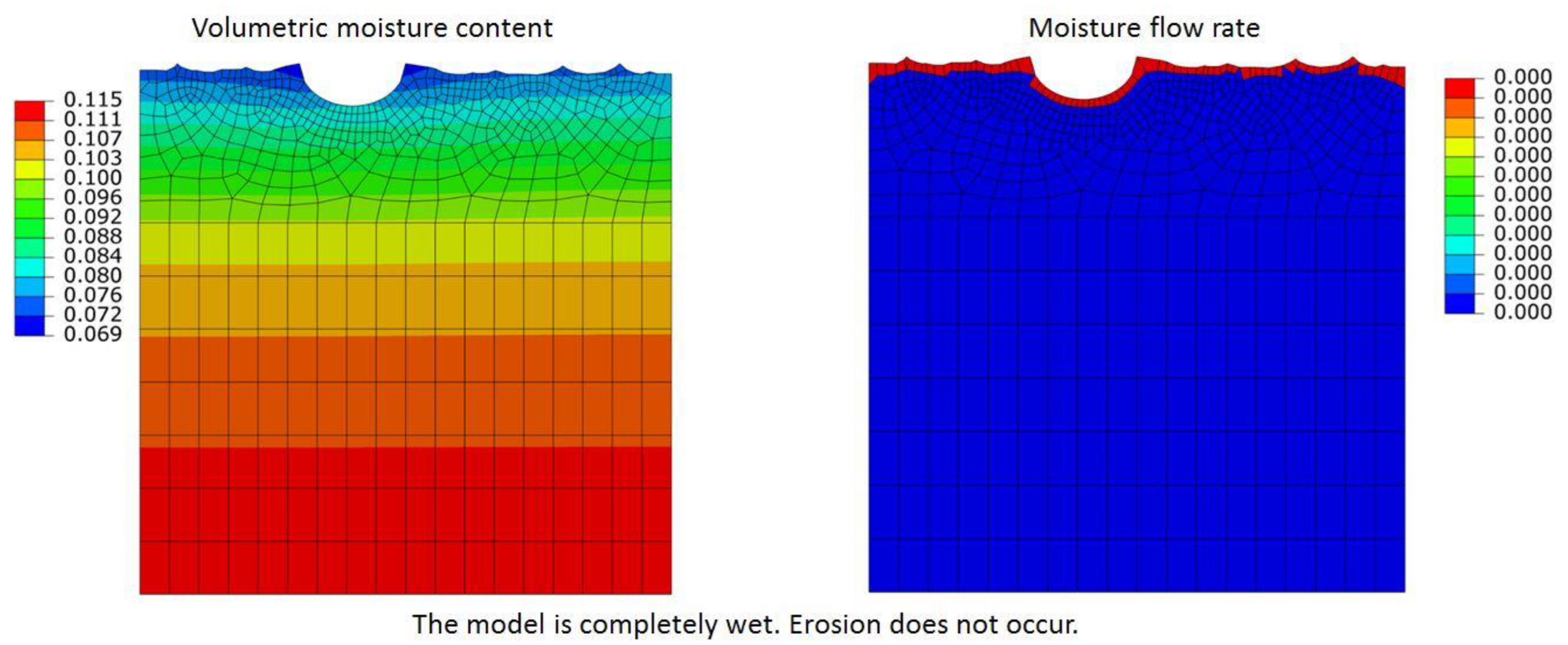
| 0.115 | No erosion |
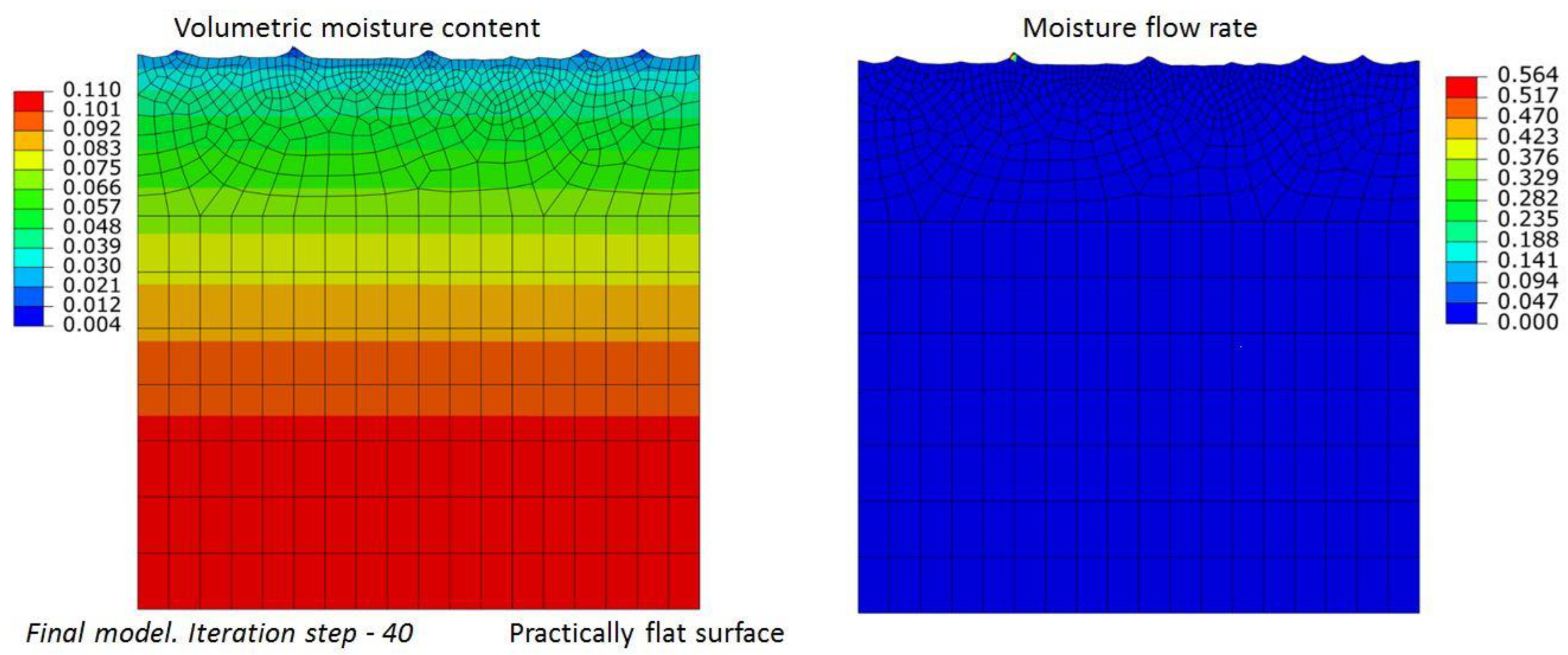
| 0.110 | Flat surface |
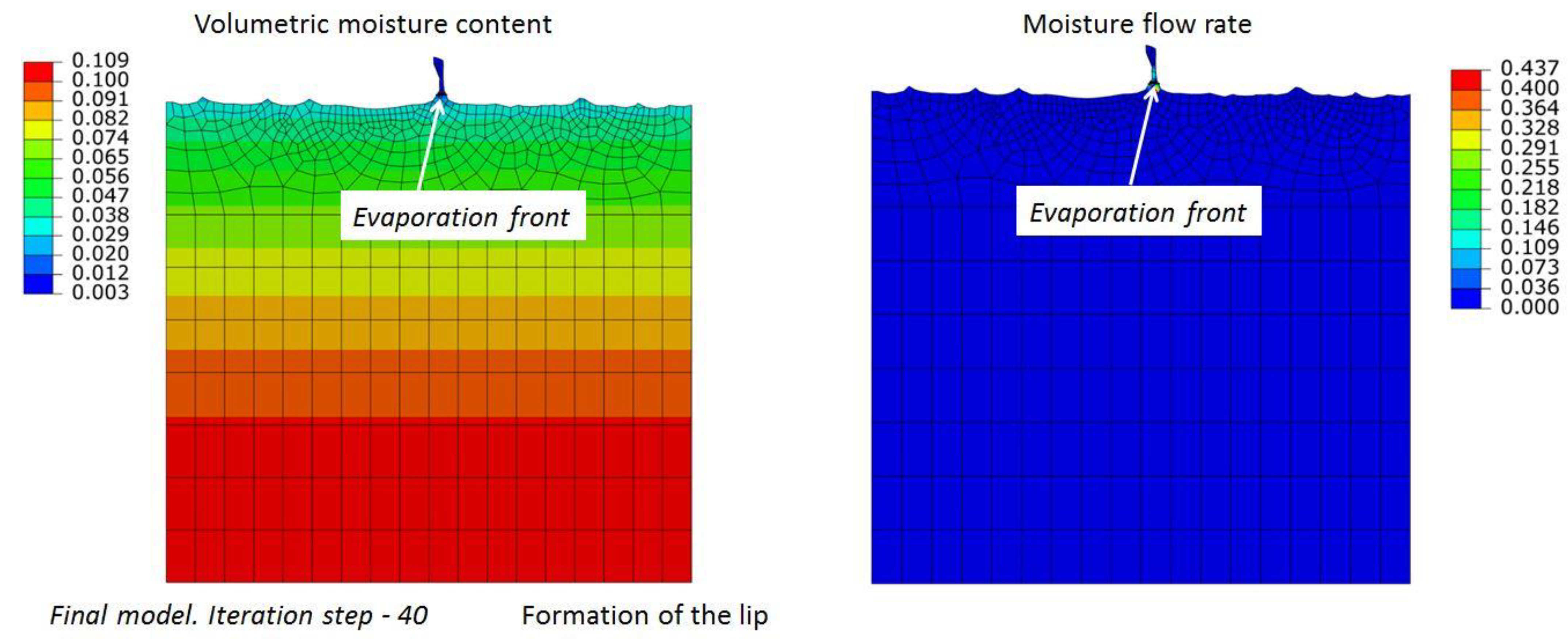
| 0.109 | Formation of single isolated lip (honeycombs) |
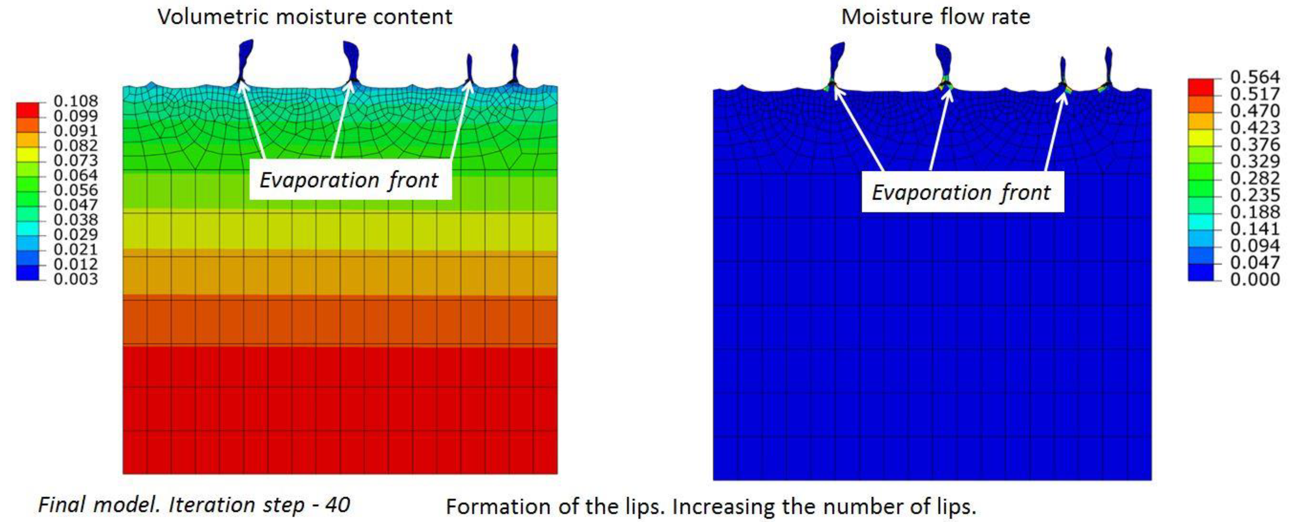
| 0.108 | Formation of several isolated lips (honeycombs) |
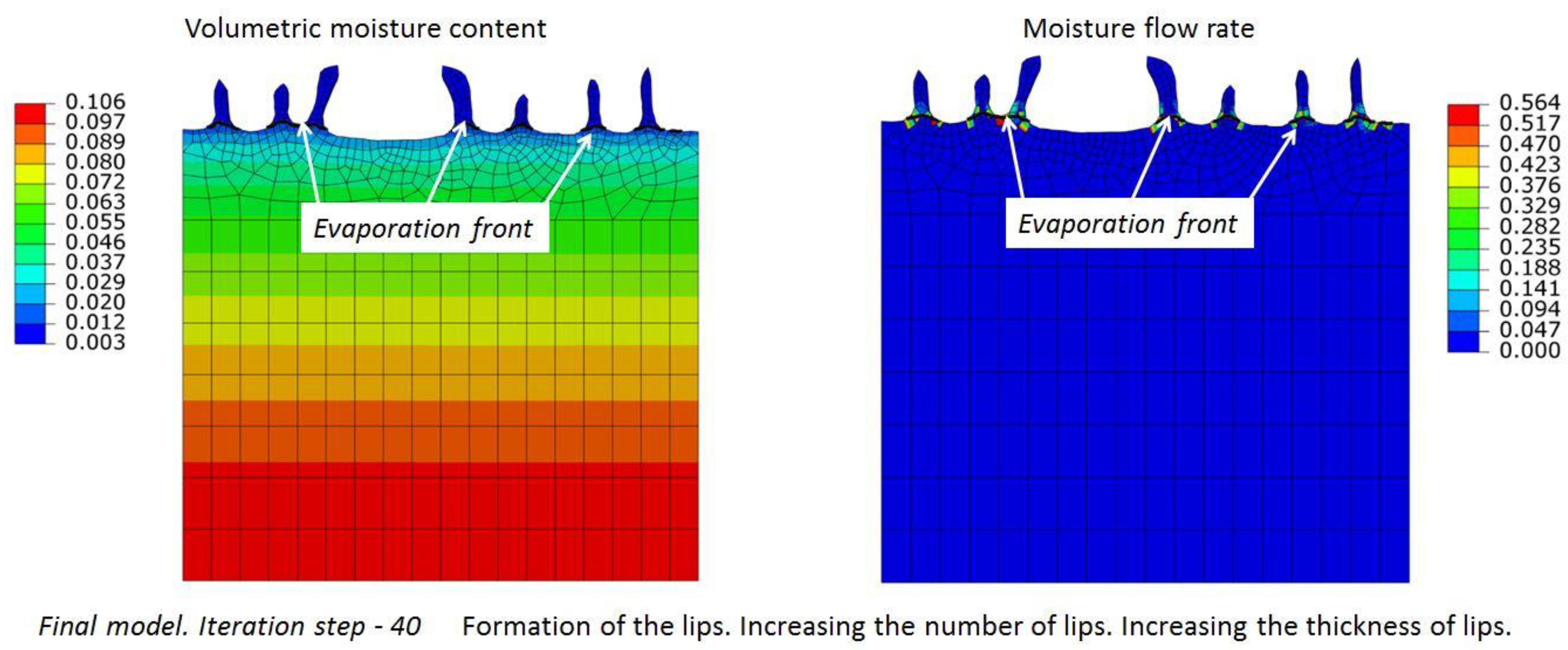
| 0.106 | Increase in number and thickness of lips (honeycombs) |
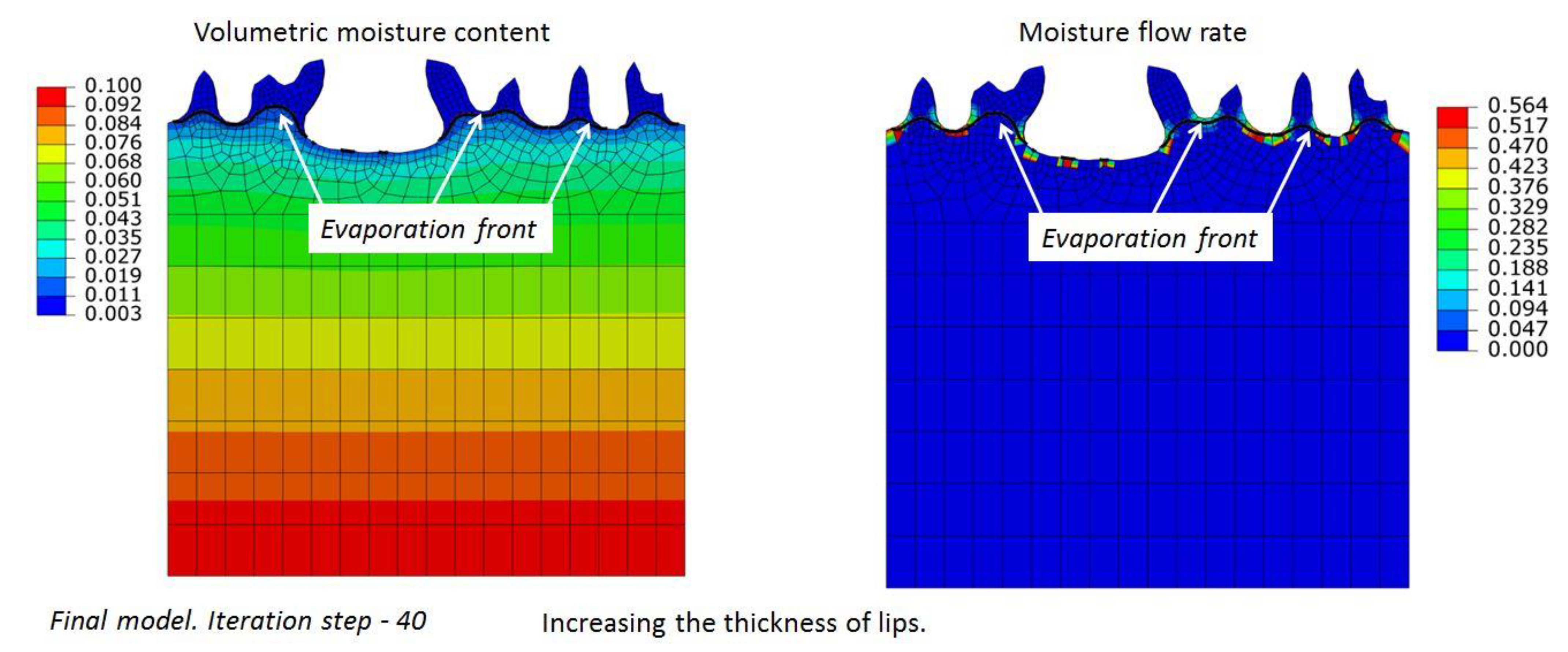
| 0.100 | Further increase in lips thickness merging of several adjacent lips (honeycombs) |
| 0.060 | Formation of deep isolated pit (tafoni) |
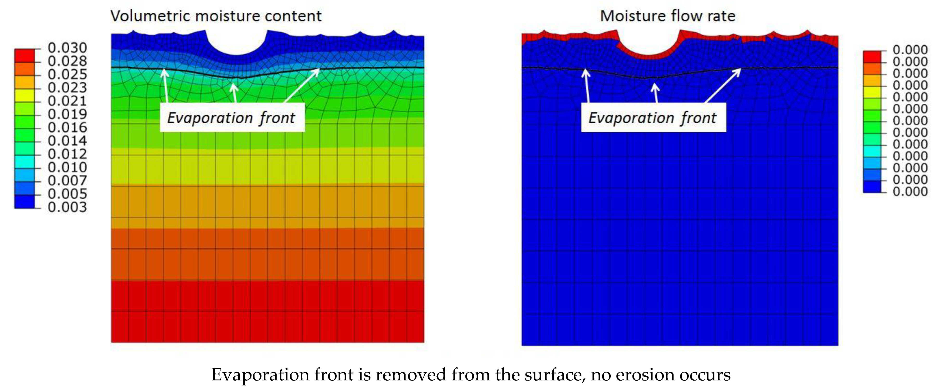
| 0.030 | No erosion |
Disclaimer/Publisher’s Note: The statements, opinions and data contained in all publications are solely those of the individual author(s) and contributor(s) and not of MDPI and/or the editor(s). MDPI and/or the editor(s) disclaim responsibility for any injury to people or property resulting from any ideas, methods, instructions or products referred to in the content. |
© 2023 by the authors. Licensee MDPI, Basel, Switzerland. This article is an open access article distributed under the terms and conditions of the Creative Commons Attribution (CC BY) license (https://creativecommons.org/licenses/by/4.0/).
Share and Cite
Safonov, A.; Minchenkov, K. Mathematical Simulation of Honeycomb Weathering via Moisture Transport and Salt Deposition. Geosciences 2023, 13, 161. https://doi.org/10.3390/geosciences13060161
Safonov A, Minchenkov K. Mathematical Simulation of Honeycomb Weathering via Moisture Transport and Salt Deposition. Geosciences. 2023; 13(6):161. https://doi.org/10.3390/geosciences13060161
Chicago/Turabian StyleSafonov, Alexander, and Kirill Minchenkov. 2023. "Mathematical Simulation of Honeycomb Weathering via Moisture Transport and Salt Deposition" Geosciences 13, no. 6: 161. https://doi.org/10.3390/geosciences13060161