Article

Factors Contributing to the Long-Term Sea Level Trends in the Iberian Peninsula and the Balearic and Canary Islands

1
Instituto Español de Oceanografía, Consejo Superior de Investigaciones Científicas (IEO-CSIC), Centro Oceanográfico de Málaga, Puerto Pesquero de Fuengirola s/n, 29640 Fuengirola, Málaga, Spain
2
Instituto Español de Oceanografía, Consejo Superior de Investigaciones Científicas (IEO-CSIC), Servicios Centrales, Calle Corazón de María, 8, 28002 Madrid, Spain
3
Instituto Mediterráneo de Estudios Avanzados, Consejo Superior de Investigaciones Científicas, Calle Miquel Marquès, 21, 07190 Esporles, Islas Baleares, Spain
*
Author to whom correspondence should be addressed.
Geosciences 2023, 13(6), 160; https://doi.org/10.3390/geosciences13060160
Submission received: 6 May 2023 / Revised: 24 May 2023 / Accepted: 29 May 2023 / Published: 31 May 2023
(This article belongs to the Special Issue Relative Sea-Level Rise)

Abstract

:
We present an attempt to estimate the long-term changes in Relative Sea Level (RSL), in addition to the different factors contributing to such trends on a local and regional scale, using a statistical linear model. The time series analysis corresponded to 17 tide-gauges, grouped in three different areas: the northern and western Atlantic coasts of the Iberian Peninsula, the Canary Islands, and the southern and eastern coasts of the Iberian Peninsula and Balearic Islands. The analysis was performed for two periods: 1948–2019, using tide-gauge data; and 1993–2019, using both tide-gauge and altimetry data for comparison. The trends for the period 1948–2019 ranged between 1.09 ± 0.14 (Canary Islands) and 2.05 ± 0.21 mm/yr for the northern and western Atlantic Iberian Peninsula. Altimetry data during the period 1993–2019 yielded quite homogeneous results for all the locations and regions, ranging between 2.7 ± 0.4 and 3.0 ± 0.3 mm/yr. In contrast, the results obtained from tide-gauge data for this recent period showed a large dispersion, very likely due to local effects, or perhaps even to levelling or instrumental errors. Nevertheless, when the results were averaged for each area, the observed trends were comparable to the altimetry results, with values of 2.3 ± 0.8, 2.7 ± 0.5, and 2.8 ± 0.8 mm/yr for the three regions of study. A stepwise forward linear regression was used to relate the observed RSL variability to the atmospheric forcing and the thermosteric and halosteric components of the sea level. Surprisingly, the thermosteric and halosteric contributions were not significantly correlated to the observed RSL in many cases; consequently, the steric, the total addition of mass, the mass of salt, and the freshwater contributions to the observed sea level trends could not be reliably estimated. This result seems to have been the consequence of the scarcity of temperature and salinity data; this hypothesis was confirmed, with the exception of the tide-gauge data for L’Estartit. This location is close to a well sampled region. In this case, the atmospheric variables and the thermosteric and halosteric terms accounted for 80% of the observed RSL variance, and the contributions of these terms could be estimated. The freshwater contribution for this location was between 1.3 and 1.4 mm/yr, consistent with recent estimations of the contributions of glaciers and Greenland and Antarctica Ice Sheets. These results highlight the importance of monitoring programs and routine sampling for the determination of the different factors contributing to the sea level variability.

1. Introduction

Rising sea levels are among the most important threats caused by climate change on coastal areas. Despite the uneven distribution of tide gauges with long time series, global mean sea level has been reconstructed during the twentieth and twenty first centuries by means of Reduced Space Optimal Interpolation [1,2,3,4,5] and Optimal Statistical Interpolation [6]. These works (in addition to the recent use of altimetry data) have revealed that the global mean sea level increased at a rate of 1.7 mm/yr [1.3 to 2.2 mm/yr] from 1901 to 2018, and this rate has accelerated to 3.7 mm/yr [3.2 to 4.2 mm/yr] for the period 2006–2018 [7,8]. The main causes of sea levels rising were the ocean warming and the melting of glaciers, in addition to the melting of Greenland and Antarctica’s Ice Sheets [9,10,11]. However, changes in the global mean sea level cannot be representative of local or regional changes [8,12], and the assessment of such changes is of paramount importance for establishing adaptation strategies [13].
Changes in local mean sea level can be decomposed into a mass component (manometric sea-level change) and a density component (steric sea-level change) [14,15]. The latter can be further decomposed into thermosteric and halosteric sea-level changes. Although the halosteric contribution is considered to be negligible on a global scale [14,16], it could have a great importance on a local or regional one [17], and in such concentration basins as the Mediterranean Sea [15,18,19]. The mass component of sea level can be inferred by subtracting the steric contribution from the observed sea level, or more recently (since the launch of the GRACE mission in 2002) from gravimetry measurements. Nevertheless, the gravimetry data have a coarse resolution of 300 km [20] and therefore cannot be used for local or even regional studies. For instance, in the case of the Mediterranean Sea, the authors of [19] found that while these data could be used to infer the mass component for the whole Mediterranean Sea, they were not suitable for smaller spatial scales.
The main goal of this study was to analyze the long-term trends of relative sea level change (RSLC) on a local scale in the north, west, and south Atlantic coasts of the Iberian Peninsula, the Canary Islands, and the Spanish Mediterranean coasts, including the Balearic Islands. Long time series from tide gauges were used for the analysis of the period 1948–2019, and both tide-gauge data and altimetry data (in this case relative to the reference ellipsoid and geocentric sea-level change, respectively [14]) were compared for the more recent period of 1993–2019. Previous studies have corrected the observed sea level for the atmospheric forcing by means of barotropic 2D models, forced using realistic pressure and wind fields [21,22,23,24]. The thermosteric and halosteric contributions to RSLC were calculated from vertical profiles of temperature and salinity compiled in different data bases or from reanalysis projects [15,25,26]. In this study, we followed a different approach, which had already been used in [27]. Monthly time series of atmospheric pressure, the zonal and meridional components of the wind, and the thermosteric and halosteric contributions were calculated from different databases. Then, a multiple linear regression was used to determine which factors contributed to the sea level variability, and to estimate their contributions to the observed sea level trends. Section 2 describes the data used and the methodology applied. Section 3 presents the results, and finally a discussion and summary of the main results are presented in Section 4.

2. Materials and Methods

2.1. Sea Level Data

Monthly time series of Revised Local Reference (RLR) sea level were downloaded from the Permanent Service for Mean Sea Level (PSMSL; https://www.psmsl.org/data/obtaining/, accessed on 1 September 2021 [28]). We downloaded the 84 respective time series, corresponding to the tide gauges distributed along the coasts of the Iberian Peninsula, the Balearic Islands, and the Canary Islands. These time series had been updated until 2018 or 2019 in most of the cases. The main objective of this work was to study long-term changes in sea level, and to determine those factors which contribute to such changes. Therefore, only time series starting in 1990 or earlier were selected for their analysis. The only exceptions to this rule were the Las Palmas and Palma time series, which started in 1991 and 1997, respectively. These shorter series have been included in order to have some information about the sea level variability in the Balearic and Canary Islands, where long time series are very scarce. The black dots in Figure 1 show the position of the 17 tide gauges selected for their analysis.
The PSMSL carried out a quality control of data and labelled those data that are suspicious. Such data have been discarded for this study. Isolated spikes with changes larger than 250 mm were also rejected. The selected time series presented some gaps, which have been filled by interpolating them with natural cubic splines when they were shorter than three months [1]. Larger gaps were filled by means of linear regression on nearby tide gauges ([27] and supplementary material). Open circles in Figure 1 show the location of tide gauges whose time series were not long enough to be considered for analysis, but which could be used for filling the gaps in the long ones. In some cases, the open circles coincided with the black dots. This is due to the existence of two tide gauges in the same location being operated by different institutions. In these cases, the longest time series was taken, while the shortest one was used for completing (or even extending) the long one.
There were four exceptions to the data processing method described above; in the case of the Cádiz time series, we used the record recovered by [29] after a very thorough analysis of its data archaeology, during which some problems of levelling were detected and corrected. Alicante and Santander time series were those reconstructed by [30]. Finally, in the case of Tenerife, we used the time series reconstructed by [31]. The latter extends until 2012 and was completed until 2019 using the data from the PSMSL. In the case of Alicante, there are two different tide gauges with available long time series. One is located in the inner harbor, and the other one is in the outer one. Finally, we analyzed the series corresponding to the outer harbor (because it had a larger extension) and used those from the inner harbor to fill some gaps. A detailed description of the regression analysis used to fill the gaps and statistical information is presented in supplementary material (including Figures S1 and S2, and Table S1). These time series have different starting dates and extend to either 2018 or 2019.
Sea level data from tide gauges are affected by Glacial Isostatic Adjustment [32,33]. The GIA contribution to the RSL at each location was obtained from the files available at the PSMSL [33,34,35], and are presented in the first column of Table 1.

2.2. Altimetry Data

Relative Sea Level data from tide gauges are affected by a Glacial Isostasy Adjustment (GIA; [32,33]), and should be corrected for this effect. Besides GIA, other land movements can also impact RSLC (for instance, tectonic subsidence/uplift or groundwater extraction, etc.; see [9]) and should be corrected by means of Global Navigational Positioning System (GNPS; [36,37]). However, no GPS measurements were available for most of the tide gauges used in this work. Altimetry data are also influenced by the GIA, but not by other land movements. Therefore, a comparison of sea level trends estimated from tide gauges and altimetry data could provide some information on the existence of such movements.
Altimetry gridded sea level anomalies were downloaded from the Copernicus Marine Service (https://resources.marine.copernicus.eu/products, accessed on 2 April 2022). We used the product Global Ocean gridded L4 Sea Surface Heights, and derived variables (SEALEVEL_GLO_PHY_L4_MY_008_047). This dataset included monthly sea level data, referred to a reference ellipsoid, and has a spatial resolution of 0.25° × 0.25° in latitude and longitude. We selected the grid points closest to each of the 17 tide gauges considered in this study, and then obtained the corresponding monthly time series. These time series extended from 1993 to 2021. Unlike tide gauge observations, altimetry data were corrected for the effect of the atmospheric forcing by means of a barotropic 2D model, forced using atmospheric pressure and wind fields [24].

2.3. Temperature and Salinity Data

Various sources of temperature and salinity data were used to compute the density component of sea level. First, gridded temperature and salinity data were obtained from the Met Office Hadley Centre observations datasets (version EN.4.2.1; [38]). This data set offered monthly data on a 1° × 1° grid with 42 vertical levels. Monthly temperature and salinity profiles were obtained for the closest grid points to each of the 17 tide gauges selected for analysis. Monthly time series of steric (ΔηST), thermosteric (ΔηT), and halosteric (ΔηH) sea-level changes (in addition to the level of salt contributions to RSLC) were estimated for each of these 17 grid points, following [15,19,27]:
Δ η S T = 1 ρ S H η Δ ρ ( z ) d z
Δ η T = 1 ρ S H η ρ 0 α Δ T ( z ) d z
Δ η H = 1 ρ S H η ρ 0 β Δ S ( z ) d z
Δ η S = 1 ρ S H η Δ S ( z ) d z
where ρS is sea surface density, η is the sea surface elevation above an arbitrary reference level, α and β are the thermal expansion and haline contraction coefficients, and ρ, S and T are the density, salinity, and temperature along the water column. We finally obtained 17 monthly time series of steric, thermosteric, halosteric, and the mass of salt components for the sea level variability, corresponding to the 17 tide gauges selected for their analysis. These time series extended from 1940 to 2019.
For comparison, a similar gridded data set has also been used, available through the NCAR/UCAR Research Data Archive [39,40].
Both data bases described above were interpolated onto regular grids, thus sharing similar characteristics and limitations, especially in coastal waters. Therefore, individual continuous profiles have also been used in such cases where they were available and consistent over time. In particular, in the case of the Mediterranean region, the thermosteric and halosteric contributions were also calculated using the data from the seasonal monitoring program RADMED [41]. The RADMED monitoring program consists of four campaigns per year, including CTD profiles in all the oceanographic stations. Such stations extend along the Spanish Mediterranean shelf, slope, and the deep waters from Málaga to Barcelona, including the Balearic Islands (see [41] for the details of this monitoring program).

2.4. Atmospheric Variables

Atmospheric forcing is one of the causes of sea level variability. This effect can be separated from others using 2D numerical models, forced using realistic atmospheric pressure and wind fields [22,23,24,42]. In this work, we statistically analyzed this forcing. For this purpose, we downloaded monthly time series of atmospheric pressure and the U and V components of the wind from the reanalysis of the National Centre for Environmental Prediction/ National Centre for Atmospheric Research (NCEP/NCAR, [43]). U and V stood for the zonal and meridional components of the wind, respectively, being U positive when directed eastwards and V when directed northwards. This data set had a spatial resolution of 2.5° × 2.5°. As in previous cases, the grid points closest to the position of the tide gauges were selected. Finally, 17 monthly time series were obtained for each variable (P, U, V) and each tide gauge. These time series extended from 1948 to 2019.

2.5. Data Processing

The long-term changes in RSLC were analyzed for the 17 locations marked as black dots in Figure 1. For each location the following monthly time series were compiled: RSL from tide gauges; altimetry sea level from altimeters; steric, thermosteric and halosteric sea-level change (ηST, ηT, and ηH) calculated from temperature and salinity profiles; and, finally, the atmospheric pressure (P), in addition to the zonal (U) and meridional (V) components of the wind, from reanalysis data. All these time series were deseasoned, removing the mean seasonal cycle; to do so for each variable, the data were grouped for each of the 12 months of the year, and mean values were calculated. These 12 values represent the climatological or average seasonal cycle for each variable. Then, the seasonal cycles were subtracted from the monthly times series; finally, the time series of anomalies or residuals were obtained, with the same length as the original ones.

2.6. Statistical Model

The statistical approach followed in this study is the same as that used in [27]. To summarize it here, we considered that the deseasoned sea level anomalies (η) depended on both the variability of the meteorological forcing (P, U, V) and the thermosteric and halosteric sea level changes (ηT, ηH). Thereafter, the sea level anomalies were named as the dependent variable, and P, U, V, ηT, ηH were the predictors or independent variables, from which the seasonal cycle had also been subtracted. Sea level anomalies also contained a part which was independent of the predictors (O). Hence, we could model the sea level variability as:
η = a + b 1 P + b 2 U + b 3 V + b 4 η T + b 5 η H + O
O represents all the other factors that are not accounted for by the other terms in (5). This included the local mass addition component of sea level (manometric sea level change: freshwater and salt), land movements (including GIA), and errors or noise.
Predictors will vary on different time scales. We assumed that such variability could be decomposed into a linear trend (representing the average change over time scales longer than the length of the time series), as well as shorter time scales that included monthly, interannual, and decadal variability:
P = a P + b P t + z P
U = a U + b U t + z U
V = a V + b V t + z V
η T = a T + b T t + z T
η H = a H + b H t + z H
O = a O + b O t + z O
where t is time, and zP, zU, zV, zT and zH are the monthly time series of predictors deseasoned and detrended. The part of η not accounted for by the atmospheric forcing, and the steric contribution can also be affected by a linear trend. In fact, the GIA contribution can be simply modeled as a linear trend for many applications. Other contributions, such as the addition of fresh water and salt, will be made of a linear trend and a term (zO) expressing the monthly and interannual variability, which we cannot calculate directly.
Substituting expressions (6) to (11) into (5), the sea level variability can be expressed as:
η = a + b t + b 1 z P + b 2 z U + b 3 z V + b 4 z T + b 5 z H + z O
Being:
b = b 1 b P + b 2 b U + b 3 b V + b 4 b T + b 5 b H + b O
The first step was to estimate the linear trends for the five deseasoned predictors, so as to obtain both deseasoned and detrended time series. Then, coefficients a, b, b1, b2, b3, b4, b5 were estimated using a stepwise forward linear regression of the deseasoned sea level on time, as well as on the five deseasoned and detrended predictors (for tide gauges and for altimetry). Notice that the stepwise regression did not necessarily include all the predictors, and that only such predictors that contributed significantly to the variance of the independent variable were finally selected (a detailed description of this method can be seen in [44], for instance).
Once the coefficients of the selected predictors had been determined, the contribution of each predictor to the linear trend of η could be estimated as the product of that coefficient times the slope of the linear trends in Equations (6) to (10) (b1bP, b2bU, b3bV, b4bT, b5bH). After correcting b for the GIA [33], bO should represent the mass addition contribution (unless there were other vertical land movements). It could be estimated as being b minus the sum of the previous contributions. Confidence intervals in the 95% confidence level were calculated for each coefficient in expressions (6) to (10) and (12). Using these confidence intervals, the uncertainty for each contribution to the sea level trend was calculated using the formula for the error propagation.
It is worth noting that the contribution of the mass of salt to sea level was not included as a potential predictor. This will be discussed further, below.

3. Results

3.1. Sea Level Linear Trends

Black lines in Figure 2 show the time series of deseasoned sea level residuals from tide gauges and from altimetry measurements. This figure and its continuation corresponded to the northern and western Atlantic coasts of the Iberian Peninsula and the Canary Islands. Figure 3 shows similar results for the Gulf of Cádiz (southern Atlantic coast of the Iberian Peninsula) and the Spanish Mediterranean coast. The left columns in Figure 2 and Figure 3 are the results from tide gauge data and the period 1948–2019. The central columns corresponded to the tide gauge data for the period 1993–2019, and the right columns present the results for the altimetry data and the period 1993–2019, with each row corresponding to a different location. The linear trends estimated for each time series, and their confidence intervals in the 95% confidence level, have been inserted in these figures. These linear trends have been corrected for the effect of GIA, and are also presented in the second column of Table 1 and Table 2. The GIA contribution to the RSLC for each location is presented in the first column of Table 1. Trends and confidence intervals in all the tables are presented with two significant figures when they were ≤25, and rounded to one single figure when they were >25. Table 1 shows those significant results obtained from tide gauge data corresponding to the period 1948–2019. Table 2 shows the results from tide gauge and altimetry data for the period 1993–2019.
Considering the period 1948–2019, with the only exception of Gibraltar, all tide gauges showed positive trends ranging from 0.59 ± 0.16 (Arrecife) to 2.29 ± 0.22 mm/yr (A Coruña). For the period 1993–2019, most tide gauges showed, as expected, positive trends that ranged between 1.3 ± 0.8 mm/yr (Leixoes) and 4.7 ± 0.7 mm/yr (Tarifa and Gibraltar). The linear trends estimated from altimetry data had a lower dispersion, ranging between 2.4 ± 0.4 mm/yr at Algeciras and Ceuta, and 4.1 ± 0.4 at Málaga (note that altimetry trends at Palma were lower than altimetry trends in other locations, but they were estimated for the period 1997–2019). Initially, the sea level trend from the Vigo tide gauge presented a negative value. This negative trend was caused by a drop in sea level since 1998. This decreasing trend was not observed in nearby tide gauges, neither in altimetry data. There is another tide gauge, named Vigo II by the PSMSL, which has operated since 1993 and which had not been used initially, as it was not necessary. The sea level from Vigo II showed positive trends for the period 1998–2019, similar to what was observed in other tide gauges located in the same region. For this reason, data for Vigo after 1998 were discarded and instead reconstructed using regression on the redundant tide gauge (Vigo II). Once this period was corrected, the Vigo trend yielded a positive value for the periods 1948–2019 and 1993–2019 (see Table 1 and Table 2). Therefore, these will be the results discussed hereafter. The results from Gibraltar are also suspicious (or simply erroneous) and will not be considered for further discussion.

3.2. Linear Trends of the Atmospheric Forcing, and the Thermosteric and Halosteric Sea-Level Change

Columns 3 to 7 in Table 1 and Table 2 show the linear trends for atmospheric pressure (column 3), both the zonal (or U (column 4)) and meridional (or V (column 5)) components of the wind, and the thermosteric (column 6) and halosteric (column 7) sea-level change. These trends are presented only in those cases that are statistically significant with a 95% confidence level. Table 1 corresponds to the period 1948–2019, and Table 2 is for the period 1993–2019.
For the period 1948–2019, atmospheric pressure increased with a trend of 0.02 ± 0.01 mbar/yr. The U and V components of the wind did not experience significant trends in most of the cases. The thermosteric contribution increased in all the locations. Nevertheless, the halosteric contribution was negative (with the only exceptions being Santander and Arrecife), significantly decreasing the final value of the steric contribution to the sea level long-term variability (see Table S2 in the supplementary material for the trends of the steric component). Notice that the steric contribution was not strictly the sum of the thermosteric and halosteric ones. Nevertheless, comparison to the steric component, estimated by means of the equation (1) and the sum of (2) and (3), showed that this was a valid approximation, and that the nonlinear terms in the equation of state of sea water were negligible for this purpose.

3.3. Linear Model

The deseasoned sea level time series from tide gauge and altimetry data were regressed on time, the atmospheric variables, and the thermosteric and halosteric sea-level changes, according to Equation (12). The regression was performed both for the period 1948–2019, and for the period 1993–2019. The model selected different variables in each case, depending on the location, the period of time, and the type of sea level data considered. Table 3 shows the coefficients for the selected predictors for the regression corresponding to the period 1948–2019. In this case, the results were estimated only from tide gauge data. The multiple correlation coefficient (R) has also been included. The square of this coefficient expresses the percentage of variance of the dependent variable that is accounted for by the linear model. Table 4 presents the coefficients for the linear model and the multiple correlation coefficients for the regression corresponding to the period 1993–2019. In this case, two different sets of coefficients were obtained: one for the tide gauge data, and another one for the altimetry data.
The atmospheric pressure was always selected as a predictor for the sea level variability measured by means of tide gauges. These coefficients were always negative and were close to −10 mm/mbar for the two periods of time analyzed. The U and V components of the wind also had a significant influence on the sea level variability in most of the tide gauges. The magnitude and sign of these coefficients depended on the location. The along coast component of the wind produced changes in the RSL in accordance with the expected upwelling or downwelling processes. Therefore, positive values of the zonal component of the wind (westerlies) induced a sea level decrease in the southern coast of the Iberian Peninsula, which is evidenced by the negative coefficients associated with the predictor U at Cádiz, Tarifa, Algeciras, and Málaga (the values associated with tide gauges can be seen in Table 3 and Table 4). On the contrary, this coefficient was positive for the Santander tide gauge. In this case, the positive U component induced downwelling and sea level rise, according to the orientation of the coast. Along the west coast of the Iberian Peninsula, it was the meridional component of the wind that produced the upwelling processes. In these cases, the coefficients of the predictor V were positive, as positive values of the wind (southerlies) induce downwelling and sea level rise.
Despite the fact that altimetry data were corrected for the atmospheric forcing, there was a statistical contribution of the atmospheric pressure and the U and V components of the wind to the sea level variability inferred from altimetry data. Nevertheless, the coefficients were lower than in the case of the tide gauge data, and especially in the case of the atmospheric pressure.
The thermosteric and halosteric contributions to sea level were selected using the linear model in some cases, not showing any clear pattern. It is noteworthy that these coefficients were always lower than one in those cases when these predictors entered the model (see discussion section). It could be argued that the thermosteric and halosteric contributions are negatively correlated. In the case that these two variables were highly correlated (collinearity), the opposite effects of these two predictors on sea level could prevent these variables from being selected in the linear model. For this reason, the halosteric component was regressed on the thermosteric one. The percentage of the variance explained ranged between 11% and 47%, with a mean value for the 17 tide gauges of 32%. Furthermore, the Variance Inflation Factor (VIF) was calculated for each predictor to check for a possible collinearity. This statistic was never over two, and therefore the collinearity of the predictors was acceptable. Furthermore, the linear model was also applied using the meteorological forcing (P, U, V) and the steric component of sea level (without decomposing it into its thermosteric and halosteric components). The steric component was never chosen when both the thermosteric and halosteric components had not been selected in the linear model of Equation (12) (see Table S3). These calculations were also repeated for all the geographical areas using the thermosteric and halosteric time series obtained from the NCAR/UCAR Research Data Archive. In the case of the Mediterranean Sea, the regression was also repeated using the temperature and salinity profiles from the monitoring program RADMED. The use of these different data sets did not improve the correlation of the thermosteric and halosteric contributions with the observed RSL.
The selected linear models explain a large fraction of the sea level variance for the two periods analyzed and both for tide gauge and altimetry data (see R values in Table 3 and Table 4). Considering the contribution of each predictor to the sea level variability (coefficients in the linear model, Table 3 and Table 4), and the linear trends of such predictors (Table 1 and Table 2), we calculated the contribution of each predictor and the mass addition contribution to the observed sea level trends (Table 5 and Table 6). The only clear contribution of the atmospheric forcing to the long-term changes of sea level was observed during the period 1948–2019, when a negative contribution (atmospheric pressure increase) was observed at all the tide gauges analyzed (Table 5). The U and V components of the wind did not contribute significantly to the sea level trends, with the only exceptions being Santander and Málaga. The thermosteric contribution for this period was positive in some tide gauges; but, in those cases, it was partially compensated by a negative halosteric contribution. Notice the negative thermosteric contribution at Leixoes (Table 5). During the period 1993–2019 (Table 6), no contribution of the atmospheric pressure was observed and there was a negative contribution of the V component of the wind at some locations. The positive contribution of the thermosteric component of sea level was observed at several locations, whereas the halosteric contribution was positive or negative depending on the location and the data set used.

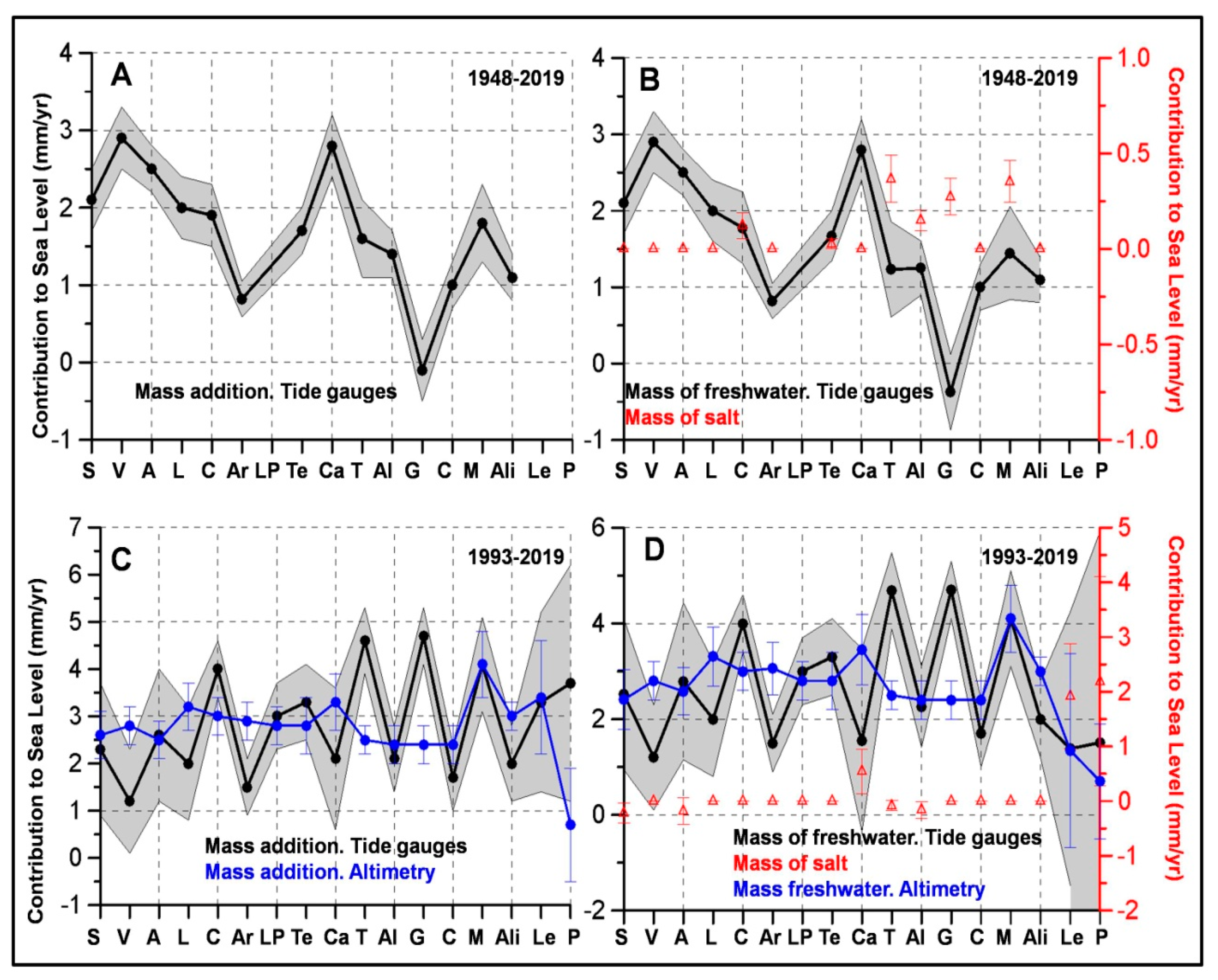
3.4. Mass of Salt and Freshwater Contributions

The mass contribution was estimated by subtracting the thermosteric, halosteric, and atmospheric contributions to the observed sea level trends that had been corrected for GIA (column #2 in Table 5 and Table 6). It can be considered that the sea level trend caused by the addition of freshwater can be estimated by subtracting the mass of salt contribution, itself estimated by means of Equation (4), from the mass contribution. The mass addition contribution experienced a clear increment during the period 1993–2019, when compared to the period 1948–2019. Nevertheless, these figures should be taken very cautiously, because of the difficulties in estimating the steric contribution. This will be discussed in detail in the next section.

4. Discussion and Conclusions

Atmospheric correction by means of the linear regression model yielded the expected results for the pressure and the alongshore component of the wind, in those cases where the coast had a clear orientation. Assuming that the sea reaches the equilibrium state after a change in pressure ΔP, the response of sea level should be:
Δ η = Δ P ρ S g
The mean surface density in the area of study ranged between 1025.9 kg/m3 at the Canary Islands, and 1027.1 kg/m3 at the northernmost tide gauges of the Mediterranean Sea. According to these values, the relation between the sea level variations and those of the atmospheric pressure should be between −9.94 and −9.95 mm/mbar (that can be rounded to −10 mm/mbar), being the well-known inverse barometer effect (see, for instance, [14]). Taking into account the uncertainty of the coefficients calculated in the linear regression, most of such coefficients were not different from the theoretical value (column 3 in Table 3 and Table 4).
It is more difficult to quantitively predict the response of sea level to the wind variability. Nevertheless, our results show a qualitative agreement with the expected upwelling and downwelling processes along the northern and southern coasts of the Iberian Peninsula, as well as on its Atlantic coast. Westerly (positive) and northerly (negative) winds induced upwelling (a decrease in sea level) on the southern and Atlantic coasts respectively. Therefore, the coefficients of the linear regression were negative in the first case and positive in the second one (see columns 4 and 5 in Table 3 and Table 4). In the northern coast of the Iberian Peninsula, westerly winds were responsible for downwelling (an increase in sea level), yielding a positive value for the coefficient of the U component of the wind at Santander. The numerical values for these coefficients showed that the sea level change for m/s of variation of the wind was comparable to the effect of sea level change for each mbar of pressure.
The atmospheric contribution to the sea-level change is frequently estimated by means of 2D barotropic circulation models [21,22,23,24]. The final validation of these results is usually achieved by calculating the variance reduction of the tide-gauge time series, or by calculating the correlation coefficients between observed sea level and that predicted using the 2D barotropic models. One study [23] found a correlation ranging between 0.6 and 0.7, depending on the tide gauge considered, and another [42] found correlations as high as 0.8. If the linear model was applied, considering only the atmospheric forcing, the multiple correlation coefficients ranged between 0.49 and 0.78, with the only exception being Arrecife, where it was 0.37. In any case, the statistical model used in this work should only be considered as a complementary approach to the numerical modeling, as the response of sea-level to the atmospheric forcing could be far from linear in some cases, depending on the topography and geometry of the coast. The explanation of the coefficients of the thermosteric and halosteric contributions to sea level presents more difficulties. The sea level variability can be decomposed into a mass and a steric contribution. The latter can be divided into thermosteric and halosteric ones. This decomposition can be expressed by means of Equation (15) (see [15] for a detailed discussion of this expression and the interpretation of the different terms of it):
Δ η = 1 ρ S Δ δ m δ A + H η α Δ T d z H η β Δ S d z
where δm is the mass in a water column of area δA. The first term in the right-hand side of Equation (15) is the change in sea level produced with the change in the mass per unit of area. The second and third terms are the thermosteric and halosteric contributions, as defined in (2) and (3). Let us consider that we know the monthly change in sea level at any tide gauge or position where altimetry data are available. If we also know the change that the temperature and salinity have experienced along the water column for the same location and month, we could calculate their contributions to the observed sea level variability. In other words, according to Equation (15), the coefficients that relate the thermosteric and halosteric terms and the observed sea level should be one. If we wanted to calculate the mass component of the sea level variability, we should simply subtract both contributions from the sea level change. However, the coefficients for these two predictors were always below one in the linear regression. Furthermore, in some cases the forward stepwise regression model did not select some of these predictors for explaining the variance of sea level. This simply indicates that, in those cases, the time series of thermosteric and halosteric contributions were not significantly correlated with the observed sea level. As explained in the results section, this cannot be attributed to the possible collinearity of the thermosteric and halosteric sea-level changes. Nor it can be attributed to the data base used, as similar results were obtained using the NCAR/UCAR Research Data Archive and the RADMED project data. Therefore, there are two possible explanations for this result.
First, the temperature and salinity data used for determining the steric contribution for each tide gauge or altimetry grid point corresponded to a large area of 1° × 1°. This large area does not necessarily represent the local conditions of the tide gauges. If the steric component of sea level was spatially homogeneous, it would not be a problem to use this large geographical area of 1° × 1° in our calculations. On the contrary, we cannot be sure that the same kind of sea–atmosphere interaction occurs in coastal and open sea waters, and the 1:1 relationship would not hold necessarily. We should be careful interpreting this result. It does not mean that the Equation (15) is not right, nor that Equations (2) and (3) do not represent the steric contributions to the sea level variability; it would simply mean that while the available time series of temperature and salinity profiles represent the real conditions at the open sea, they are not representative of the local changes occurring at the costal tide gauges.
This explanation has another problem; the altimetry sea level also corresponded to an open sea area similar to that representative of the temperature and salinity profiles used for the calculation of the steric contribution. In this case, the ηT and ηH predictors did not significantly correlate with the altimetry sea level in all the locations. In those cases when these predictors were selected using the linear model, the coefficients were also lower than one, as in the case of the tide gauge data.
A second explanation is that the available temperature and salinity data do not yield reliable estimations of the steric contributions, neither for the open sea areas, nor for the coastal ones. This problem has already been evidenced by [19] in the case of the Mediterranean Sea, wherein the authors pointed out that the different available data bases did not allow them to obtain consistent estimations of the steric component of the sea level, nor of the mass of salt contribution. As a consequence of this, consistent estimations of the contribution of the mass of freshwater could not be obtained. This problem arises from the scarcity of temperature and salinity data along the water column, which makes it very difficult to calculate the monthly, interannual, and long-term variability of the heat and salt content in the upper layer of the sea, where there is a very large natural variability [45,46]. The authors of [47] subsampled the results from a numerical model at the same times and locations where real temperature and salinity profiles were available. The authors interpolated the subsampled data onto a regular 3D grid on a monthly basis. Linear trends estimated from these interpolated data were not able to capture the real long-term variability of the simulated data, evidencing the limitations of the present gridded climatologies.
Taking into account all the problems related to the scarcity of data, we considered that the monthly thermosteric and halosteric contributions calculated in our study could not be the real ones, but still could have a certain correlation with them. Once again, the coefficients relating the observed sea level to the thermosteric and halosteric contributions would not be one, and we could not directly subtract such contributions to calculate the addition of mass.
Whether the first explanation is true or the second one, the degree of correlation between the observed sea level and the available steric contributions was determined with the time series themselves, and the stepwise correlation analysis. In those cases in which there was a significant correlation, the coefficients that related the observed sea level to ηT and ηH and the linear trends calculated for these predictors were used to estimate the thermosteric and halosteric contributions to the linear trends of sea level. In such cases, the salinity profiles were also used to estimate the contribution of the mass of salt. Notice that as expression (3) was not directly used to estimate the contribution of the halosteric component, it would not be consistent to use Equation (4) for the calculation of the mass of salt. If (4) was divided by (3), and neglecting the variability of β along the water column compared to the changes in ΔS, the ratio of both contributions would be as follows:
1 ρ 0 β 0
with ρ0 and β0 being some average or reference values. Therefore, the mass of salt contribution was estimated as the halosteric contribution multiplied by the factor (16). It could also be argued that the term (4) could have been included as another predictor in the linear model and the mass of salt could have been estimated directly, using linear regression. In such case the two predictors given in the Equations (3) and (4) would be proportional, and the resulting system of equations would be ill-conditioned.
For those cases in which neither ηT nor ηH were significantly correlated with the sea level, those predictors were not used to estimate the mass contribution of sea level. We have to emphasize that this does not mean that there is no steric contribution to the observed sea level, neither that there is no contribution by the mass of salt. It simply means that the available time series of steric contribution do not resemble the real ones, and therefore cannot be used for this purpose. Figure 4A (period 1948–2019) and 4C (period 1993–2019) show the mass contribution of sea level, once corrected for the atmospheric forcing. This contribution includes the addition of freshwater and salt. Figure 4B,D show the contribution of the mass of salt (red triangles) and the contribution of the mass of freshwater. In those figures corresponding to the 1993–2019 period, both the tide gauge (black lines) and the altimetry (blue lines) analyses have been included.
For the long period 1948–2019, only tide gauge data were available. The Gibraltar sea level trend was negative (see column 2 in Table 1), and so was the contribution of mass addition and freshwater (Figure 4A,B). This is not a reliable result and indicates that some sort of leveling or other such problem affected this tide gauge during this period. For this reason, this tide gauge will be excluded in the following discussion. The sea level, averaged for the whole area (and corrected for the effect of GIA), increased at a rate of 1.58 ± 0.19 mm/yr. This result is coincident with the trend observed for Global Mean Sea Level (GMSL) from 1901 to 2018, which was 1.7 mm/yr [7,8]. During this period, the atmospheric pressure had a positive trend in all the tide gauges and was therefore analyzed to have induced a decrease in the sea level. However, the behavior of the thermosteric and halosteric contributions (in addition to that of the addition of mass of salt) had different values for the different geographical areas analyzed. Averaging the results for the Atlantic coast of the Iberian Peninsula (northern and western coasts), the RSLC was 2.05 ± 0.21 mm/yr. It was observed that the warming and salting of the water column produced positive and negative trends for the thermosteric and halosteric sea-level changes. Nevertheless, there was no significant correlation between these terms and the observed RSLC. Hence, the thermosteric, halosteric, and mass of salt terms did not contribute significantly to the RSLC, and the addition of mass and that of freshwater were the same and larger than the observed RSLC (2.3 ± 0.4 mm/yr).
This is an unrealistic result. The water column has warmed during the period 1948–2019 (see column 6 in Table 1). Although the halosteric term had a negative trend that could partially counterbalance the thermosteric one, it was also associated with a positive contribution of the term of the mass of salt. Therefore, the warming of the oceans, having absorbed 90% of the heat stored by the Earth Climate System [48], should have contributed to the RSLC as observed on a global scale [9]. The lack of correlation between our ηT, ηH time series and the RSL did not allow us to use them for the calculation of their contribution to the sea level trends. It could be argued that while the available thermosteric and halosteric time series are not able to reproduce the monthly and interannual variability of sea level, they still could capture its long-term variability. In that case, we could simply subtract the thermosteric and halosteric trends from the sea level trend to obtain that of the mass component. This would be equivalent to accept that the coefficients relating ηT and ηH to sea level are lower than one for the monthly and interannual time scales, but they are equal to one for the longer time scales. Similarly, the mass of salt could be directly subtracted to the mass component to assess the change in the mass of freshwater. When these calculations were carried out, the results were unrealistic, with negative freshwater contributions in some cases.
In the case of the Canary Islands, for this period of time (1948–2019) the RSL increased at a rate of 1.09 ± 0.14 mm/yr, with a mass contribution of 1.3 ± 0.3 mm/yr. Once again the analysis of the steric and salt contributions did not yield significant results. Finally, in the case of the southern Atlantic Iberian coast and that of the Mediterranean Sea, the sea level trend was 1.35 ± 0.18 mm/yr, which as similar to that obtained for the Western Mediterranean by [6] (1.2 ± 0.14 mm/yr). The thermosteric and the mass of salt contributions were positive, and the halosteric one was negative, yielding the contributions of 1.6 ± 0.4, 0.15 ± 0.05, and 1.5 ± 0.4 mm/yr for the mass, mass of salt, and mass of freshwater contributions, respectively. These results were more in agreement with other works that estimate that the addition of fresh water on a global scale is higher than 1 mm/yr [49] or 1.31 mm/yr [9]. Nevertheless, it should be taken into account that these latter estimations correspond to the 1990s decade and the first decade of the present century, whilst our results are calculated for a longer period of time.
The discussion above suggests that the available temperature and salinity data are not suitable for the analysis of the monthly, interannual, and long-term variability of the steric and mass of salt components of sea level. This would support those results in [19,47]. The authors of [46] also showed that the available temperature and salinity data collected in the Mediterranean Sea during the second half of the twentieth century (and the first decades of the twenty-first) could not capture the long-term trends of these variables at the upper layer of the sea because of the scarcity of data, combined with the large natural variability of this layer. Despite the data scarcity problem, it should be considered that these tide gauges are not provided with GNSS receivers. As no altimetry data are available for comparison during this period, other problems such as vertical land movements, or changes in the location of the instruments, that have not been properly documented, should not be discarded.
Both tide gauges and altimetry data are available for the period 1993–2019. The comparison of these results shows that trends estimated from altimetry data were quite homogeneous (see Table 5 and Table 6, and the blue lines in Figure 4). When averaging for the whole area of study, the RSL increased at a rate of 2.8 ± 0.3 mm/yr with mass, salt, and freshwater contributions of 2.8 ± 0.5, 0.10 ± 0.09, and 2.7 ± 0.6 mm/yr, respectively. The results obtained from the analysis of tide gauge data were much more variable, reflecting possible local effects or even errors in the instrumentation. However, these effects were canceled when the results were averaged, and the trends estimated for RSL, mass, salt, and freshwater contributions were similar to those calculated from altimetry data: 2.5 ± 0.7, 2.7 ± 1.1, 0.25 ± 0.25, and 2.5 ± 1.4 mm/yr, respectively.
During this recent period, there were no contributions from the atmospheric forcing. Although these variables were significantly correlated with the observed sea level (Table 4), the atmospheric pressure did not show any long-term trend, whereas the U and V components of the wind increased in some cases and decreased in others. The agreement between the altimetry and tide gauge results confirmed the acceleration of the sea level trends during recent decades, but once again the observed sea level was not significantly correlated to the thermosteric and halosteric components in most of the cases. Consequently, the linear model was not able to estimate the steric contribution, nor can it estimate the mass, salt, and freshwater ones. Nevertheless, it is worth considering the particular case of L’Estartit. It is well known that the WMED has undergone a warming process throughout the twentieth century which has accelerated with the beginning of the twenty-first. Therefore, the thermosteric component should contribute not only to the monthly and interannual variability of the sea level variability, but also to its long-term trend (see column 6 in Table 6), as observed on a global scale [7,8,9]. On the other hand, this sea has also suffered an intense salinity increase [18,46,50], and there should thus be a negative contribution of the halosteric component and a positive one of the mass of salt (column 7 in Table 6 and Figure 4D). In this case, all the predictors (both those representing the atmospheric forcing (P, U, V) and the thermosteric and halosteric components) contributed to the observed sea level variability (see Table 4 and Table 6). Furthermore, the linear model had a multiple correlation coefficient of 0.88, which means that the model was able to explain 77% of the sea level variance. Hence, we can be confident that the different contributions to the long-term trends of the sea level were accurately estimated. These results indicate that the sea level increased at L’Estartit at a rate of 2.7 ± 0.8 mm/yr since 1993. The atmospheric forcing was significantly correlated with the RSL and explained part of the monthly and interannual variability; however, as these variables did not experience any long-term trend during the period 1993–2019, they did not contribute to the sea level linear trend. The thermosteric and halosteric contributions were positive and negative, as expected, and the resulting mass addition had a positive trend of 3.3 ± 1.9 mm/yr. The mass of salt contribution was 1.9 ± 1.0 mm/yr and the freshwater contribution was 1.4 ± 2.9 mm/yr for the tide-gauge data, and 1.3 ± 2.0 for the altimetry ones. The large uncertainty in the latter component arose from the formula for the expansion of errors. As the trend for the mass of freshwater is derived from the subtraction of the mass of salt from the mass component, its uncertainty is the sum of both errors. However, the obtained value was close to those recently reported by [9,49], based on the melting of glaciers and of Greenland and the Antarctic’s ice sheets; the authors estimated this contribution as being 1.31 mm/yr. Furthermore, in the case of L’Estartit, the estimations of the sea level linear trends (and its different components), were almost the same when calculated from tide gauge or altimetry data. Our hypothesis is that the good behavior of the statistical model for L’Estartit arises from the quality of the data. First, the tide gauge started operating in recent decades (1990) with no location changes or any other known problem. Beside this, its location is very close to an area very intensively sampled by different monitoring programs [51] and has received considerable attention because of its proximity to the area of formation of Western Mediterranean Deep Water.
In summary, averaging for all the tide gauges, it can be stated that the sea level increased at a rate of 1.58 ± 0.19 mm/yr from 1948 to 2019. The large dispersion of these results, based on the analysis of tide-gauge data, makes it difficult to estimate differences between the three large geographical areas analyzed: the Atlantic Iberian Peninsula, the Canary Islands, and the Southern Peninsula and Spanish Mediterranean Sea. The trends of sea level accelerated during the period 1993–2019. The results for the three areas (for both tide-gauge and altimetry data) were very similar (indistinguishable within the uncertainty level) and range from 2.3 ± 0.8 to 3.0 ± 0.3 mm/yr. The available data did not allow us to estimate the thermosteric and halosteric contributions in a reliable way, and therefore the mass and salt components could not be estimated. According to previous works, this seems to be the result of the data scarcity. By contrast, the results from L’Estartit, (which is located in a well sampled area) allowed us to estimate the positive and negative contributions of the thermosteric and halosteric components of sea level, and the mass of salt. The mass of freshwater at this location increased at a rate of 1.4 ± 2.9 mm/yr for tide gauge data, and 1.3 ± 2.0 mm/yr for the altimetry data, in agreement with recent observations derived from glacier ice melting. These results evidence once more the importance of the monitoring systems of the oceans for estimating the different contributions to the present sea level rise.

Supplementary Materials

The following supporting information can be downloaded at: https://www.mdpi.com/article/10.3390/geosciences13060160/s1, Method for filling the gaps in long time series, Figure S1: Reconstruction of sea level time series at Algeciras; Figure S2: Reconstruction of sea level time series at Vigo; Table S1: Column #1 shows the long time series that are analyzed in this work. Column #2 shows the predictors or time series that are used to fill the gaps in the long time series. In some cases there are two different lines. This means that different predictors have been used for different gaps. For instance, one gap in Santander time series was filled with data from Bilbao, and another gap was filled with data from Pasaia. The third column shows the multiple correlation coefficient for the regression of the dependent variable on the predictors.; Table S2: Linear trends for the steric sea level change; Table S3: Coefficients and multiple regression coefficient for the forward stepwise regression of sea level on time, P, U, V, and the steric sea-level change (without decomposing it into its thermosteric and halosteric components).

Author Contributions

Conceptualization, M.V.-Y., E.T. and M.M.; methodology, M.V.-Y., F.M., M.C.G.-M., E.B. and C.A.; software, M.V.-Y.; writing—original draft preparation, M.V.-Y.; writing—review and editing, F.M., E.B., C.A. and M.C.G.-M.; project administration, M.C.G.-M. All authors have read and agreed to the published version of the manuscript.

Funding

This research received no external funding.

Data Availability Statement

Sea level data were obtained from the PSMSL, where data are freely available. Altimetry data are freely available from the COPERNICUS Marine Service. Temperature and salinity data are available from the Met Office Hadley Centre and the NCAR/UCAR, and atmospheric data are available from the NCEP/NCAR.

Conflicts of Interest

The authors declare no conflict of interest.

References

  1. Calafat, F.M.; Chambers, D.P.; Tsimplis, M.N. On the ability of global sea level reconstructions to determine trends and variability. J. Geophys. Res. Ocean. 2014, 119, 1572–1592. [Google Scholar] [CrossRef]
  2. Llovel, W.; Cazenave, A.; Rogel, P.; Lombard, M.; Bergé-Nguyen, A. 2-D reconstruction of past sea level (1950–2003) using tidegauge records and spatial patterns from a general ocean circulation model. Clim. Past Discuss. 2009, 5, 1109–1132. [Google Scholar]
  3. Church, J.A.; White, N.J. A 20th century acceleration in global sea level rise. Geophys. Res. Lett. 2006, 33, L01602. [Google Scholar] [CrossRef]
  4. Church, J.A.; White, N.J. Sea-level rise from late 19th to early 21st century. Surv. Geophys. 2011, 32, 585–602. [Google Scholar] [CrossRef]
  5. Church, J.A.; White, N.J.; Coleman, R.; Lambeck, K.; Mitrovica, J.X. Estimates of the Regional Distribution of Sea Level Rise overthe 1950–2000 Period. J. Clim. 2004, 17, 2609–2625. [Google Scholar] [CrossRef]
  6. Ramos-Alcántara, J.; Gomis, D.; Jordà, G. Reconstruction of Mediterranean coastal sea level at different timescales based on tide gauge records. Ocean Sci. 2022, 18, 1781–1803. [Google Scholar] [CrossRef]
  7. Fox-Kemper, B.; Hewitt, H.T.; Xiao, C.; Aðalgeirsdóttir, G.; Drijfhout, S.S.; Edwards, T.L.; Golledge, N.R.; Hemer, M.; Kopp, R.E.; Krinner, G.; et al. Ocean, Cryosphere and Sea Level Change. In Climate Change 2021: The Physical Science Basis; Contribution of Working Group I to the Sixth Assessment Report of the Intergovernmental Panel on Climate Change; Masson-Delmotte, V.P., Zhai, A., Pirani, S.L., Connors, C., Péan, S., Berger, N., Caud, Y., Chen, L., Goldfarb, M.I., Gomis, M., et al., Eds.; Cambridge University Press: Cambridge, UK; New York, NY, USA, 2021; pp. 1211–1362. [Google Scholar] [CrossRef]
  8. Arias, P.A.; Bellouin, N.; Coppola, E.; Jones, R.G.; Krinner, G.; Marotzke, J.; Naik, V.; Palmer, M.D.; Plattner, G.K.; Rogelj, J.; et al. Technical Summary. In Climate Change 2021: The Physical Science Basis; Contribution of Working Group I to the Sixth Assessment Report of the Intergovernmental Panel on Climate Change; Masson-Delmotte, V.P., Zhai, A., Pirani, S.L., Connors, C., Péan, S., Berger, N., Caud, Y., Chen, L., Goldfarb, M.I., Gomis, M., et al., Eds.; Cambridge University Press: Cambridge, UK; New York, NY, USA, 2021; pp. 33–144. [Google Scholar] [CrossRef]
  9. Oppenheimer, M.; Glavovic, B.C.; Hinkel, J.; van de Wal, R.; Magnan, A.K.; Abd-Elgawad, A.; Cai, R.; Cifuentes-Jara, M.; DeConto, R.M.; Ghosh, T.; et al. Sea Level Rise and Implications for Low-Lying Islands, Coasts and Communities. In IPCC Special Report on the Ocean and Cryosphere in a Changing Climate; Pötner, H.-O., Roberts, D.C., Masson-Delmotte, V., Zhai, P., Tignor, M., Poloczanska, E., Mintenbeck, K., Alegri, A., Nicolai, M., Okem, A., et al., Eds.; Cambridge University Press: Cambridge, UK; New York, NY, USA, 2019; pp. 321–445. [Google Scholar] [CrossRef]
  10. Dangendorf, S.; Marcos, M.; Wöppelmann, G.; Conrad, T.; Frederikse, C.P.; Riva, R. Reassessment of 20th Century Global Mean Sea Level Rise. Proc. Natl. Acad. Sci. USA 2017, 114, 5946–5951. [Google Scholar] [CrossRef]
  11. Dangendorf, S.; Marcos, M.; Müller, A.; Zorita, E.; Riva, R.; Berk, K.; Jensen, J. Detecting anthropogenic footprints in sea level rise. Nat. Commun. 2015, 6, 7849. [Google Scholar] [CrossRef]
  12. Gomis, D.; Tsimplis, M.; Marcos, M.; Fenoglio-Marc, L.; Pérez, B.; Raicich, F.; Vilibic, I.; Wöppelmann, G.; Monserrat, S. Mediterranean Sea-Level Variability and Trends. In The Climate of the Mediterranean Region: From the Past to the Future; Lionello, P., Ed.; Elsevier: Amsterdam, The Netherlands, 2012. [Google Scholar]
  13. BongartsLebbe, T.; Rey-Valette, H.; Chaumillon, É.; Camus, G.; Almar, R.; Cazenave, A.; Claudet, J.; Rocle, N.; Meur-Férec, C.; Viard, F.; et al. Designing Coastal Adaptation Strategies to Tackle Sea Level Rise. Front. Mar. Sci. 2021, 8, 740602. [Google Scholar] [CrossRef]
  14. Gregory, J.M.; Griffies, S.M.; Hughes, C.W.; Lowe, J.A.; Church, J.A.; Fukimori, I.; Gomez, N.; Kopp, R.E.; Landerer, F.; Le Cozannet, G.; et al. Concepts and Terminology for Sea Level: Mean, Variability and Change, Both Local and Global. Surv. Geophys. 2019, 40, 1251–1289. [Google Scholar] [CrossRef]
  15. Jordà, G.; Gomis, D. On the interpretation of the steric and mass components of sea level variability: The case of the Mediterranean Sea. J. Geophys. Res. Ocean. 2013, 118, 953–963. [Google Scholar] [CrossRef]
  16. Gregory, J.M.; Lowe, J.A. Predictions of global and regionalsea-level rise using AOGCMs with and without flux adjustment. Geophys. Res. Lett. 2000, 27, 3069–3072. [Google Scholar] [CrossRef]
  17. Wang, G.; Cheng, L.; Boyer, T.; Li, C. Halosteric Sea Level Changes during the Argo Era. Water 2017, 9, 484. [Google Scholar] [CrossRef]
  18. Tsimplis, M.N.; Baker, T.F. Sea level drop in the Mediterranean Sea: An indicator of deep water salinity and temperature changes? Geophys. Res. Lett. 2000, 27, 1731–1734. [Google Scholar] [CrossRef]
  19. Jordà, G.; Gomis, D. Reliability of the steric and mass components of Mediterranean sea level as estimated from hydrographic gridded products. Geophys. Res. Lett. 2013, 40, 3655–3660. [Google Scholar] [CrossRef]
  20. Camargo, C.M.L.; Riva, R.E.M.; Hermans, T.H.J.; Slangen, A.B.A. Trends and Uncertainties of Regional Barystatic Sea-level Change in the Satellite Altimetry Era. Earth Syst. Dynam. Discuss 2021, preprint. [Google Scholar] [CrossRef]
  21. Tsimplis, M.N.; Spada, G.; Marcos, M.; Fleming, N. Multidecadal sea level trends and land movements in the Mediterranean Seawith estimates of factors perturbing tide gauge data and cumulative uncertainties. Glob. Planet. Chang. 2011, 76, 63–76. [Google Scholar] [CrossRef]
  22. Gomis, D.; Ruiz, S.; Sotillo, M.G.; Álvarez-Fanjul, E.; Terradas, J. Low frequency Mediterranean sea level variability: Thecontribution of atmospheric pressure and wind. Glob. Planet. Chang. 2008, 63, 215–229. [Google Scholar] [CrossRef]
  23. Marcos, M.; Tsimplis, M.N. Forcing of coastal sea level rise patterns in the North Atlantic and the Mediterranean Sea. Geophys. Res. Lett. 2007, 34, L18604. [Google Scholar] [CrossRef]
  24. Carrère, L.; Lyard, F. Modeling the barotropic response of the global ocean to atmospheric wind and pressure forcing—Comparisons with observations. Geophys. Res. Lett. 2003, 30, 1275. [Google Scholar] [CrossRef]
  25. Storto, A.; Bonaduce, A.; Feng, X.; Yang, C. Steric Sea Level Changes from Ocean Reanalyses at Global and Regional Scales. Water 2019, 11, 1987. [Google Scholar] [CrossRef]
  26. Church, J.A.; Roemmich, D.; Domingues, C.M.; Willis, J.K.; White, N.J.; Gilson, J.E.; Stammer, D.; Köhl, A.; Chambers, D.P.; Landerer, F.W.; et al. Ocean Temperature and Salinity Contributions to Global and Regional Sea-Level Change. In Understanding Sea-Level Rise and Variability; Church, J.A., Woodworth, P.L., Aarup, T., Wilson, W.S., Eds.; Cambridge University Press: Cambridge, UK, 2010; pp. 143–176. [Google Scholar]
  27. Vargas-Yáñez, M.; Tel, E.; Moya, F.; Ballesteros, E.; García-Martínez, M.C. Long-Term Changes, Inter-Annual, and Monthly Variability of Sea Level at the Coasts of the Spanish Mediterranean and the Gulf of Cádiz. Geosciences 2021, 11, 350. [Google Scholar] [CrossRef]
  28. Holgate, S.J.; Matthews, A.; Woodworth, P.L.; Rickards, L.J.; Tamisiea, M.E.; Bradshaw, E.; Foden, P.R.; Gordon, K.M.; Jevrejeva, S.; Pugh, J. New Data Systems and Products at the Permanent Service for Mean Sea Level. J. Coast. Res. 2013, 29, 493–504. [Google Scholar] [CrossRef]
  29. Marcos, M.; Puyol, B.; Wöppelmann, G.; Herrero, C.; García-Fernández, M.J. The long sea level record at Cádiz (Southern Spain). J. Geophys. Res. 2011, 116, C12003. [Google Scholar] [CrossRef]
  30. Marcos, M.; Puyol, B.; Gómez, B.P.; Fraile, M.A.; Talke, S.A. Historical tide-gauge sea level observations in Alicante and Santander (Spain) since the 19th century. Geosci. Data J. 2021, 82, 144–153. [Google Scholar] [CrossRef]
  31. Marcos, M.; Puyol, B.; Calafat, F.M.; Woppelmann, G. Sea level changes at Tenerife Island (NE Tropical Atlantic) since 1927. J. Geophys. Res. Ocean. 2013, 118, 4899–4910. [Google Scholar] [CrossRef]
  32. Whitehouse, P.L. Glacial isostatic adjustment modelling: Historical perspectives, recent advances, and future directions. Earth Surf. Dynam. 2018, 6, 401–429. [Google Scholar] [CrossRef]
  33. Peltier, W.R. Global Glacial Isostacy and the surface of the ice-age Earth: The ICE-5G (VM2) Model and GRACE. Annu. Rev. Earth Planet. Sci. 2004, 32, 111–149. [Google Scholar] [CrossRef]
  34. Peltier, W.R. Postglacial Variations in the Level of the Sea: Implications for Climate Dynamics and Solid-Earth Geophysics. Rev. Geophys. 1998, 36, 603–689. [Google Scholar] [CrossRef]
  35. Peltier, W.R. On the Hemispheric Origins of Meltwater Pulse 1A. Quat. Sci. Rev. 2005, 24, 1655–1671. [Google Scholar] [CrossRef]
  36. Santamaría-Gómez, A.; Gravelle, M.; Dangendorf, S.; Marcos, M.; Spada, G.; Wöppelmann, G. Uncertainty of the 20th century sea-level rise due to vertical land motion errors. Earth Planet. Sci. Lett. 2017, 473, 24–32. [Google Scholar] [CrossRef]
  37. Kleinherenbrink, M.; Riva, R.; Frederikse, T. A comparison of methods to estimate vertical land motion trends from GNSS and altimetry at tide gauge stations. Ocean Sci. 2018, 14, 187–204. [Google Scholar] [CrossRef]
  38. Good, S.A.; Martin, M.J.; Rayner, N.A. Quality controlled ocean temperature and salinity profiles and monthly objective analyses with uncertainty estimates. J. Geophys. Res. Ocean. 2013, 118, 6704–6716. [Google Scholar] [CrossRef]
  39. Ishii, M.; Kimoto, M.; Sakamoto, K.; Iwasaki, S. Steric sea level changes estimated from historical ocean subsurface temperatureand salinity analyses. J. Oceanogr. 2006, 62, 155–170. [Google Scholar] [CrossRef]
  40. Ishii, M.; Kimoto, M.; Sakamoto, K.; Iwasaki, S. Subsurface Temperature and Salinity Analyses. Available online: https://rda.ucar.edu/datasets/ds285.3/ (accessed on 19 August 2021).
  41. López-Jurado, J.L.; Balbín, R.; Alemany, F.; Amengual, B.; Aparicio-González, A.; Fernández de Puelles, M.L.; García-Martínez, M.C.; Gazá, M.; Jansá, J.; Morillas-Kieffer, A.; et al. The RADMED Monitoring Programme as a Tool for MSFD Implementation: Towards an Ecosystem-Based Approach. Ocean. Sci. 2015, 11, 897–908. [Google Scholar] [CrossRef]
  42. Gomis, D.; Tsimplis, M.N.; Martí-Mínguez, B.; Ratsimandresy, A.W.; García-Lafuente, J.; Josey, S.A. Mediterranean Sea level and barotropic flow through the Strait of Gibraltar for the period 1958–2001 and reconstructed since 1659. J. Geophys. Res. 2006, 111, C11005. [Google Scholar] [CrossRef]
  43. Kalnay, E.; Kanamitsu, M.; Kistler, R.; Collins, W.; Deaven, D.; Gandin, L.; Iredell, M.; Saha, S.; White, G.; Woollen, J.; et al. The NCEP/NCAR 40-year reanalysis project. Bull. Am. Meteorol. Soc. 1996, 77, 437–472. [Google Scholar] [CrossRef]
  44. Draper, N.R.; Smith, H. Applied Regression Analysis, 2nd ed.; Wiley: New York, NY, USA, 1981. [Google Scholar]
  45. Vargas-Yáñez, M.; Moya, F.; Balbín, R.; Santiago, R.; Ballesteros, E.; Sánchez-Leal, R.F.; Romero, P.; Carmen, G.-M.M. Seasonal and Long-Term Variability of the Mixed Layer Depth and its Influence on Ocean Productivity in the Spanish Gulf of Cádiz and Mediterranean Sea. Front. Mar. Sci. 2022, 9, 901893. [Google Scholar] [CrossRef]
  46. Vargas-Yáñez, M.; García-Martínez, M.C.; Moya, F.; Balbín, R.; López-Jurado, J.L.; Serra, M.; Zunino, P.; Pascual, J.; Salat, J. Updating temperature and salinity mean values and trends in the Western Mediterranean: The RADMED Project. Prog. Oceanogr. 2017, 157, 27–46. [Google Scholar] [CrossRef]
  47. Llasses, J.; Jordà, G.; Gomis, D. Skills of different hydrographic networks in capturing changes in the Mediterranean Sea at climate scales. Clim. Res. 2015, 63, 1–18. [Google Scholar] [CrossRef]
  48. Von Schuckmann, K.; Cheng, L.; Palmer, M.D.; Hansen, J.; Tassone, C.; Aich, V.; Adusumilli, S.; Beltrami, H.; Boyer, T.; Cuesta-Valero, F.J.; et al. Heat stored in the Earth system: Where does the energy go? Earth Syst. Sci. Data 2020, 12, 2013–2041. [Google Scholar] [CrossRef]
  49. Zemp, M.; Huss, M.; Eckert, N.; Thibert, E.; Paul, F.; Nussbaumer, S.U.; Gärtner-Roer, I. Brief communication: Ad hoc estimation of glacier contributions to sea-level rise from the latest glaciological observations. Cryosphere 2020, 14, 1043–1050. [Google Scholar] [CrossRef]
  50. Borghini, M.; Bryden, H.; Schroeder, K.; Sparnocchia, S.; Vetrano, A. The Mediterranean is becoming saltier. Ocean Sci. 2014, 10, 693–700. [Google Scholar] [CrossRef]
  51. Coppola, L.; Raimbault, P.; Mortier, L.; Testor, P. Monitoring the Environment in the Northwestern Mediterranean Sea. Eos Trans. Am. Geophys. Union Am. Geophys. Union (AGU) 2019, 100, 10. [Google Scholar] [CrossRef]
Figure 1. Black dots show the position of tide gauges, with long time series used for their analysis. Black circles show those tide gauges with short time series, which were unsuitable for the analysis of long-term trends, but which were used for filling or extending the long time series.
Geosciences 13 00160 g001
Figure 2. Time series of sea level anomalies for the northern and western coasts of the Iberian Peninsula, and the Canary Islands. Black lines show the time series of sea level anomalies and red lines show the regression on the predictors selected using the stepwise forward linear regression. Each row corresponds to a different location: Santander (AC), Vigo (DF), A Coruña (GI), Leixoes (JL), Cascais (MO), Arrecife (PR), Las Palmas (S,T) and Tenerife (UW). The left, central, and right columns correspond to the tide gauge data for the period 1948–2019, tide gauge data for the period 1993–2019, and altimetry data for the period 1993–2019, respectively. Linear trends, corrected for GIA, have been inserted.
Geosciences 13 00160 g002aGeosciences 13 00160 g002b
Figure 3. Time series of sea level anomalies for the southern Atlantic coast of the Iberian Peninsula, and the Spanish Mediterranean coast (including the Balearic Islands). Black lines show the time series of sea level anomalies and red lines show the regression on the predictors selected using the stepwise forward linear regression. Each row corresponds to a different location: Cádiz (AC), Tarifa (DF), Algeciras (GI), Ceuta (JL), Málaga (MO), Alicante (PR), L’Estartit (S,T) and Palma (U,V). The left, central, and right columns correspond to the tide gauge data for the period 1948–2019, tide gauge data for the period 1993–2019, and altimetry data for the period 1993–2019, respectively. Linear trends, corrected for GIA, have been inserted.
Geosciences 13 00160 g003
Figure 4. (A) shows the contribution to the sea level linear trends of the addition of mass (black lines). (B) shows the contribution to the sea level linear trends of the addition of freshwater (black line) and the mass of salt (red triangles). Both (A,B) correspond to the period 1948–2019 and the 17 tide gauges analyzed. Shaded areas and red vertical bars are the 95% confidence intervals. (C,D) show similar results for the period 1993–2019. In these cases, black lines correspond to the analysis of the 17 tide gauges, and the blue lines to the analysis of the altimetry data from the 17 grid points closest to the tide gauges. In all the cases the x-axis shows the initial of the tide gauges: Santander (S), Vigo (V), A Coruña (A), Leixoes (L), Cascais (C), Arrecife (Ar), Las Palmas (LP), Tenerife (Te), Cádiz (C), Tarifa (T), Algeciras (Al), Gibraltar (G), Ceuta (C), Málaga (M), Alicante (Ali), L’Estartir (Le), and Palma (P).
Geosciences 13 00160 g004
Table 1. Linear trends for the period 1948–2019. Column 1 indicates the location and the relative sea level contribution, using a GIA obtained from the PSMSL [33,34,35]. Column 2 presents sea level trends for tide gauge data. Columns 3 through 7 show those significant trends for the atmospheric pressure, the U component of the wind, the V component of the wind, as well as the thermosteric and halosteric contributions to sea level, respectively. Linear trends for sea level at column 2 have been corrected for the effect of GIA.
PeriodLinear Trends (b ± 95% CI). Tide Gauges.
1948–2019Sea Level
b
Pressure
bP
U-Wind
bU
V-Wind
bV
Thermost.
BT
Halost.
BH
Location (GIA)mm/yrdbar/yrms−1/yrms−1/yrmm/yrmm/yr
Santander
(−0.11)
2.08 ± 0.210.02 ± 0.01 0.01 ± 0.010.01 ± 0.000.62 ± 0.100.36 ± 0.15
Vigo
(−0.12)
2.66 ± 0.240.02 ± 0.01 1.72 ± 0.16−1.41 ± 0.18
A Coruña
(0.0)
2.29 ± 0.220.02 ± 0.01 1.18 ± 0.14−0.78 ± 0.17
Leixoes
(−0.2)
1.61 ± 0.200.02 ± 0.01 1.78 ± 0.17−1.41 ± 0.19
Cascais
(−0.07)
1.62 ± 0.190.02 ± 0.01 1.98 ± 0.20−1.26 ± 0.24
Arrecife
(0.01)
0.59 ± 0.160.02 ± 0.01 0.01 ± 0.010.96 ± 0.15
Las Palmas
(0.05)
Tenerife
(0.09)
1.59 ± 0.120.02 ± 0.01 0.02 ± 0.001.19 ± 0.12−0.32 ± 0.13
Cádiz
(−0.18)
2.62 ± 0.210.02 ± 0.01−0.01 ± 0.01 1.43 ± 0.12−1.16 ± 0.25
Tarifa
(−0.18)
1.38 ± 0.210.02 ± 0.01 1.48 ± 1.13−1.21 ± 0.25
Algeciras
(−0.19)
1.00 ± 0.140.02 ± 0.01 1.48 ± 0.13−1.21 ± 0.25
Gibraltar
(−0.19)
−0.18 ± 0.160.02 ± 0.01 1.48 ± 0.13−1.21 ± 0.25
Ceuta
(−0.18)
0.89 ± 0.150.02 ± 0.01 1.48 ± 0.13−1.21 ± 0.25
Málaga
(−0.23)
1.40 ± 0.190.02 ± 0.01 −0.01 ± 0.001.53 ± 0.13−1.51 ± 0.24
Alicante
(−0.05)
0.82 ± 0.170.02 ± 0.01 −0.01 ± 0.001.44 ± 0.09−1.91 ± 0.15
L’Estartit
(0.06)
Palma
(0.25)
Table 2. Linear trends for the period 1993–2019. Column 1 indicates the location. Column 2 presents two values; the upper one is for sea level trends estimated from tide gauge data, and the lower one from altimetry data. Columns 3 through 7 show those significant trends for the atmospheric pressure, the U component of the wind, and V component of the wind, as well as the thermosteric and halosteric contributions of sea level, respectively. Linear trends for sea level from tide gauges at column 2 have been corrected for the effect of GIA.
PeriodLinear Trends (b ± 95% CI) Tide Gauges and Altimetry.
1993–2019Sea Level bPressure bPU-Wind bUV-Wind bVThermost. bTHalost. bH
Locationmm/yrdbar/yrms−1/yrms−1/yrmm/yrmm/yr
Santander
Tide Gauge
Altimetry

2.0 ± 0.8
2.56± 0.25

−0.02 ± 0.02

−0.02 ± 0.02

1.5 ± 0.7
Vigo
Tide gauge
Altimetry

1.4 ± 0.9
2.9 ± 0.3

0.9 ± 0.8
A Coruña
Tide Gauge
Altimetry

3.0 ± 0.9
2.69 ± 0.25

1.1 ± 0.6

0.7 ± 0.7
Leixoes
Tide gauge
Altimetry

1.3 ± 0.8
3.07 ± 0.25

0.02 ± 0.02

−0.03 ± 0.02

1.0 ± 0.9
Cascais
Tide gauge
Altimetry

3.8 ± 0.5
2.8 ± 0.3

−0.05 ± 0.03
Arrecife
Tide gauge
Altimetry

1.4 ± 0.5
3.0 ± 0.3

−0.03 ± 0.02

−0.03 ± 0.02

1.0 ± 0.6
Las Palmas
Tide gauge
Altimetry

3.3 ± 0.5
2.9 ± 0.3

−0.02 ± 0.02

0.02 ± 0.02

0.8 ± 0.5
Tenerife
Tide gauge
Altimetry

3.4 ± 0.8
3.1 ± 0.3

−0.02 ± 0.02

0.02 ± 0.02

1.5 ± 0.5
Cádiz
Tide gauge
Altimetry

1.3 ± 0.9
3.2 ± 0.3

−0.03 ± 0.02

0.7 ± 0.6

2.8 ± 1.1
Tarifa
Tide gauge
Altimetry

4.7 ± 0.7
2.5 ± 0.3

2.4 ± 0.7

1.5 ± 1.2
Algeciras
Tide gauge
Altimetry

2.3 ± 0.6
2.4 ± 0.4

2.4 ± 0.7

1.5 ± 1.2
Gibraltar
Tide gauge
Altimetry

4.7 ± 0.6
2.4 ± 0.4

2.4 ± 0.7

1.5 ± 1.2
Ceuta
Tide gauge
Altimetry

1.9 ± 0.6
2.4 ± 0.4

2.4 ± 0.7

1.5 ± 1.2
Málaga
Tide gauge
Altimetry

3.7 ± 0.7
4.1 ± 0.4

0.03 ± 0.03

2.4 ± 0.7
Alicante
Tide gauge
Altimetry

2.0 ± 0.8
3.0 ± 0.3

2.9 ± 0.4

−4.2 ± 0.6
L’Estartit
Tide gauge
Altimetry

2.7 ± 0.8
2.7 ± 0.3

2.9 ± 0.3

−6.2 ± 0.4
Palma *
Tide gauge
Altimetry

2.0 ± 1.1
1.8 ± 0.5

3.7 ± 0.5

−5.9 ± 0.5
* The period for Palma time series is 1997–2019.
Table 3. Coefficients of the linear model expressed by means of equation (12). These results correspond to the tide gauge data for the period 1948–2019. Only the coefficients corresponding to the predictors selected using the stepwise forward regression have been presented. The multiple correlation coefficient, R, is also included.
PeriodCoefficients of the Linear Model for Sea Level from Tide Gauges
1948–2019Time bPressure b1U-Wind b2V-Wind b3Thermost. b4Halost. b5R
Locationmm/yrmm/mbarmm/ms−1mm/ms−1
Santander2.08 ± 0.21−9.4 ± 0.98.2 ± 2.114.9 ± 2.3 0.85
Vigo2.66 ± 0.24−11.6 ± 1.1−11.31 ± 2.320.2 ± 2.4 0.85
A Coruña2.29 ± 0.22−9.9 ± 1.0−5.4 ± 2.218.1 ± 2.3 0.84
Leixoes1.61 ± 0.20−8.2± 1.0 21.1 ± 2.1−0.10 ± 0.05 0.81
Cascais1.62 ± 0.19−11.3 ± 1.0−5.1 ± 1.44.0 ± 1.2 0.07 ± 0.040.84
Arrecife0.59 ± 0.16−9.6 ± 1.8 0.11 ± 0.070.46
Las Palmas
Tenerife1.59 ± 0.12−12.1 ± 1.3 0.14 ± 0.070.07 ± 0.060.83
Cádiz2.62 ± 0.21−12.1 ± 1.8−10.0 ± 2.56 ± 3 0.75
Tarifa1.38 ± 0.21−12.7 ± 2.0−7.9 ± 2.115 ± 70.22 ± 0.110.22 ± 0.050.64
Algeciras1.00 ± 0.14−11.8 ± 1.2−6.9 ± 1.313 ± 4 0.09 ± 0.030.72
Gibraltar−0.18 ± 0.16−10.7 ± 1.5−6.2 ± 1.718 ± 50.22 ± 0.080.17 ± 0.040.62
Ceuta0.89 ± 0.15−12.7 ± 1.3 13 ± 50.13 ± 0.06 0.70
Málaga1.40 ± 0.19−14.1 ± 1.3−11.7 ± 1.8 0.10 ± 0.090.17 ± 0.050.71
Alicante0.82 ± 0.17−13.6 ± 1.0−6.2 ± 1.87 ± 3 0.76
L’Estartit
Palma
Table 4. Coefficients of the linear model expressed by means of equation (12). These results correspond to both the tide gauge and altimetry data for the period 1993–2019. Only the coefficients corresponding to the predictors selected using the stepwise forward regression have been presented.
PeriodCoefficients ± 95% CI of the Linear Model for Sea Level from Tide Gauges and Altimetry
1993–2019Time bPressure b1U-Wind b2V-Wind b3Thermost. b4Halost. b5R
Locationmm/yrmm/mbarmm/ms−1mm/ms−1
Santander
Tide gauge
Altimetry

2.0 ± 0.8
2.56 ± 0.25

−10.0 ± 0.9
1.3 ± 0.6

10.2 ± 2.0
2.4 ± 1.3

11.7 ± 2.5
6.4 ± 1.6

0.19 ± 0.11
0.19 ± 0.07

0.10 ± 0.07
0.09 ± 0.05

0.92
0.83
Vigo
Tide gauge
Altimetry

1.4 ± 0.9
2.9 ± 0.3

−11.6 ± 1.4

−9 ± 3
−4.8 ± 1.4

18 ± 3
6.1 ± 1.4

0.27 ± 0.15
0.13 ± 0.07

0.19 ± 0.13
0.10 ± 0.06

0.83
0.81
A Coruña
Tide gauge
Altimetry

3.0 ± 0.9
2.69 ± 0.25

−9.3 ± 1.6
0.8 ± 0.6

−4 ± 3
−1.4 ± 1.3

18 ± 4
5.2 ± 1.4

0.27 ± 0.19
0.12 ± 0.07

0.18 ± 0.17
0.08 ± 0.06

0.79
0.82
Leixoes
Tide gauge
Altimetry

1.3 ± 0.8
3.07 ± 0.25

−8.3 ± 1.4
1.2 ± 0.7

21 ± 3
5.7 ± 1.4


0.12 ± 0.06


0.08 ± 0.05

0.83
0.84
Cascais
Tide gauge
Altimetry

3.8 ± 0.5
2.8 ± 0.3
−8.7 ± 1.0
−5.8 ± 1.4
−3.1 ± 1.1

4.6 ± 1.3
4.6 ± 1.0

0.89
0.80
Arrecife
Tide gauge
Altimetry

1.4 ± 0.5
3.0 ± 0.3

−7.7 ± 2.1
3.8 ± 2.4

0.19 ± 0.08


0.13 ± 0.08

0.60
0.78
Las Palmas
Tide gauge
Altimetry

3.3 ± 0.5
2.9 ± 0.3
−9.7 ± 1.8 4.2 ± 2.2
0.26 ± 0.09
0.18 ± 0.08

0.13 ± 0.08
0.11 ± 0.07

0.85
0.78
Tenerife
Tide gauge
Altimetry

3.7 ± 0.5
3.1 ± 0.3

−12 ± 2
−3.6 ± 1.8


−3.5 ± 2.2

0.21 ± 0.12
0.25 ± 0.09

0.10 ± 0.10
0.15 ± 0.08

0.79
0.78
Cádiz
Tide gauge
Altimetry

1.3 ± 0.9
3.2 ± 0.3
−9.9 ± 2.5
−8 ± 3
−3.4 ± 1.2

11 ± 5
7.0 ± 1.5


0.09 ± 0.06

−0.13 ± 0.08
0.04 ± 0.03

0.63
0.83
Tarifa
Tide gauge
Altimetry

4.7 ± 0.7
2.5 ± 0.3

−12.2 ± 1.7

−7.3 ± 1.7
−2.6 ± 1.1

25 ± 6
18 ± 3

0.04 ± 0.04

0.89
0.77
Algeciras
Tide gauge
Altimetry

2.3 ± 0.6
2.4 ± 0.4

−10.5 ± 1.6
−1.5 ± 1.5

−5.5 ± 1.6
−3.4 ± 1.5

22 ± 6
16 ± 5

0.08 ± 0.03

0.83
0.68
Gibraltar
Tide gauge
Altimetry

4.7 ± 0.6
2.4 ± 0.4

−10.8 ± 2.0
−1.5 ± 1.5

−7.2 ± 2.0
−3.4 ± 1.5

23 ± 7
16 ± 5

0.84
0.68
Ceuta
Tide gauge
Altimetry

1.9 ± 0.6
2.4 ± 0.4

−12.1 ± 1.6


−1.9 ± 1.5

18 ± 6
20 ± 5
0.08 ± 0.06
0.81
0.66
Málaga
Tide gauge
Altimetry

3.7 ± 0.7
4.1 ± 0.4

−12.1 ± 1.8

12.3 ± 2.1
−4.4 ± 1.6

8 ± 5
13 ± 4


0.06 ± 0.06

0.15 ± 0.04

0.84
0.79
Alicante
Tide gauge
Altimetry

2.0 ± 0.8
3.0 ± 0.3

−10.3 ± 1.6
−3.0 ± 1.1


−3.1 ± 1.8


5.4 ± 3.0

0.63
0.77
L’Estartit
Tide gauge
Altimetry

2.7 ± 0.8
2.7 ± 0.3

−13.5 ± 1.0
−2.9 ± 0.7

−8 ± 3

4.2 ± 2.1
3.3 ± 1.3

0.27 ± 0.14
0.3 ± 0.1

0.22 ± 0.12
0.25 ± 0.09

0.88
0.79
Palma
Tide gauge
Altimetry

2.0 ± 1.1
2.0 ± 1.1

−9.7 ± 2.0
−2.3 ± 1.1


6 ± 3


0.34 ± 0.14

0.28 ± 0.23

0.58
0.58
Table 5. Contribution of the different factors to the observed trends of sea level from tide gauge data from the period 1948–2019.
PeriodContributions to Sea Level Trends from Tide Gauges.
1948–2019Mass Add.PressureU-WindV-WindThermost.Halost.
Locationmm/yrmm/yrmm/yrmm/yrmm/yrmm/yr
Santander2.1 ± 0.4−0.20 ± 0.100.05 ± 0.040.10 ± 0.07
Vigo2.9 ± 0.4−0.22 ± 0.13
A Coruña2.5 ± 0.3−0.18 ± 0.11
Leixoes2.0 ± 0.4−0.18 ± 0.08 −0.18 ± 0.10
Cascais1.9 ± 0.4−0.22 ± 0.11 0.08 ± 0.09−0.09 ± 0.05
Arrecife0.82 ± 0.23−0.22 ± 0.07
Las Palmas
Tenerife1.7 ± 0.3−0.20 ± 0.07 0.17 ± 0.08−0.02 ± 0.02
Cádiz2.8 ± 0.4−0.23 ± 0.110.06 ± 0.06
Tarifa1.6 ± 0.5−0.27 ± 0.10 0.33 ± 0.16−0.27 ± 0.09
Algeciras1.4 ± 0.3−0.25 ± 0.08 −0.11 ± 0.04
Gibraltar−0.1 ± 0.4−0.22 ± 0.08 0.32 ± 0.12−0.20 ± 0.07
Ceuta1.0 ± 0.3−0.26 ± 0.09 0.19 ± 0.09
Málaga1.8 ± 0.5−0.29 ± 0.12 0.16 ± 0.13−0.26 ± 0.08
Alicante1.1 ± 0.3−0.25 ± 0.13 −0.04 ± 0.03
L’Estartit
Palma
Table 6. Contribution of the different factors to the observed trends of sea level from tide gauge and altimetry data from the period 1993–2019.
PeriodContributions to Sea Level Trends from Tide Gauges and Altimetry.
1993–2019Mass Add.PressureU-WindV-WindThermost.Halost.
Locationmm/yrmm/yrmm/yrmm/yrmm/yrmm/yr
Santander
Tide gauge
Altimetry

2.3 ± 1.4
2.6 ± 0.5

−0.22 ±.0.22
−0.05 ± 0.06

−0.24 ± 0.21
−0.13 ± 0.12

0.16 ± 0.13
−0.14 ± 0.09
Vigo
Tide gauge
Altimetry

1.2 ± 1.1
2.8 ± 0.4

0.24 ± 0.24
0.12 ± 0.12
A Coruña
Tide gauge
Altimetry

2.6 ± 1.4
2.5 ± 0.4

0.3 ± 0.3
0.14 ± 0.11

0.14 ± 0.18
0.06 ± 0.07
Leixoes
Tide gauge
Altimetry

2.0 ± 1.2
3.2 ± 0.5

−0.7 ± 0.4
−0.19 ± 0.12


0.08 ± 0.09
Cascais
Tide gauge
Altimetry

4.0 ± 0.6
3.0 ± 0.4

−0.21 ± 0.15
−0.21 ± 0.14
Arrecife
Tide gauge
Altimetry

1.5 ± 0.6
2.9 ± 0.4

−0.10 ± 0.11


0.12 ± 0.11
Las Palmas
Tide gauge
Altimetry

3.0 ± 0.7
2.8 ± 0.4

0.09 ± 0.09

0.21 ± 0.16
0.14 ± 0.11
Tenerife
Tide gauge
Altimetry

3.3 ± 0.8
2.8 ± 0.6


−0.07 ± 0.08

0.32 ± 0.21
0.38 ± 0.18
Cádiz
Tide gauge
Altimetry

2.1 ± 1.5
3.3 ± 0.6

−0.4 ± 0.3
−0.24 ± 0.14

−0.10 ± 0.14
0.06 ± 0.07

−0.4 ± 0.3
0.11 ± 0.10
Tarifa
Tide gauge
Altimetry

4.6 ± 0.7
2.5 ± 0.3

0.06 ± 0.07
Algeciras
Tide gauge
Altimetry

2.1 ± 0.7
2.4 ± 0.4

0.12 ± 0.11
Gibraltar
Tide gauge
Altimetry

4.7 ± 0.6
2.4 ± 0.4
Ceuta
Tide gauge
Altimetry

1.7 ± 0.7
2.4 ± 0.4

0.19 ± 0.15
Málaga
Tide gauge
Altimetry

4.1 ± 1.0
4.1 ± 0.7

−0.4 ± 0.3
−0.13 ± 0.12


0.14 ± 0.15
Alicante
Tide gauge
Altimetry

2.0 ± 0.8
3.0 ± 0.3
L’Estartit
Tide gauge
Altimetry

3.3 ± 1.9
3.4 ± 1.2

0.8 ± 0.4
0.8 ± 0.3

−1.4 ± 0.7
−1.5 ± 0.6
Palma
Tide gauge
Altimetry

3.7 ± 2.5
0.7 ± 1.2


1.3 ± 0.6

−1.6 ± 1.4
Disclaimer/Publisher’s Note: The statements, opinions and data contained in all publications are solely those of the individual author(s) and contributor(s) and not of MDPI and/or the editor(s). MDPI and/or the editor(s) disclaim responsibility for any injury to people or property resulting from any ideas, methods, instructions or products referred to in the content.

