Quantitative Long-Term Monitoring (1890–2020) of Morphodynamic and Land-Cover Changes of a LIA Lateral Moraine Section

Altmann, Moritz; Ramskogler, Katharina; Mikolka-Flöry, Sebastian; Pfeiffer, Madlene; Haas, Florian; Heckmann, Tobias; Rom, Jakob; Fleischer, Fabian; Himmelstoß, Toni; Pfeifer, Norbert; Ressl, Camillo; Tasser, Erich; Becht, Michael

doi:10.3390/geosciences13040095

Open AccessArticle

Quantitative Long-Term Monitoring (1890–2020) of Morphodynamic and Land-Cover Changes of a LIA Lateral Moraine Section

by

Moritz Altmann

^1,*

,

Katharina Ramskogler

^2,3

,

Sebastian Mikolka-Flöry

⁴

,

Madlene Pfeiffer

⁵,

Florian Haas

¹

,

Tobias Heckmann

¹

,

Jakob Rom

¹

,

Fabian Fleischer

¹,

Toni Himmelstoß

¹,

Norbert Pfeifer

⁴

,

Camillo Ressl

⁴

,

Erich Tasser

²

and

Michael Becht

¹

Department of Physical Geography, Catholic University of Eichstätt-Ingolstadt, 85072 Eichstätt, Germany

²

Institute for Alpine Environment, Eurac Research, 39100 Bolzano, Italy

³

Department of Botany, Universität Innsbruck, 6020 Innsbruck, Austria

⁴

Research Unit Photogrammetry E120.7, Department of Geodesy and Geoinformation, TU Wien, 1040 Vienna, Austria

⁵

Institute of Geography, University of Bremen, 28359 Bremen, Germany

^*

Author to whom correspondence should be addressed.

Geosciences 2023, 13(4), 95; https://doi.org/10.3390/geosciences13040095

Submission received: 28 February 2023 / Revised: 15 March 2023 / Accepted: 20 March 2023 / Published: 23 March 2023

(This article belongs to the Topic Advances in Environmental Remote Sensing)

Download

Browse Figures

Versions Notes

Abstract

:

Aerial photographs of the European Alps usually only reach back to the middle of the 20th century, which limits the time span of corresponding studies that quantitatively analyse long-term surface changes of proglacial areas using georeferenced orthophotos. To the end of the Little Ice Age, this leads to a gap of about 100 years. Using digital monoplotting and several historical terrestrial photographs, we show the quantification of surface changes of a Little Ice Age lateral moraine section until the late second half of the 19th century, reaching a total study period of 130 years (1890–2020). The (initial) gully system expands (almost) continuously over the entire study period from 1890 to 2020. Until 1953, the vegetation-covered areas also expanded (mainly scree communities, alpine grasslands and dwarf shrub communities), before decreasing again, especially between 1990 and 2003, due to large-scale erosion within the gully system. Furthermore, our results show that the land-cover development was impacted by temperature and precipitation changes. With the 130-year study period, we contribute to a substantial improvement in the understanding of the processes in the proglacial by analysing the early phase and thus the immediate response of the lateral moraine to the ice exposure.

Keywords:

aerial photos; Central Eastern Alps; digital monoplotting; historical terrestrial oblique photos; long-term mapping; paraglacial slope adjustment; proglacial area; upper Kauner Valley (Ötztal Alps)

1. Introduction

Since the end of the Little Ice Age (LIA) around the middle of the 20th century, glacier retreat in high alpine mountains, caused by global warming, has led to a continuous expansion of the glacier forelands, the so-called proglacial areas [1,2]. Glacial environments and corresponding proglacial areas are among the most rapidly changing areas on earth, as they are strongly affected by climate change. After ice release, the exposed areas, especially the steep and, to a high degree, unvegetated lateral moraines, are reworked by different geomorphological processes, such as fluvial and nival erosion, debris flows, slope failures and landslides, which can be associated with high erosion rates [3,4,5,6]. Generally, this phase is described as the paraglacial slope adjustment process, which can last several decades to centuries [7,8,9]. These processes have led to a high number of deeply incised lateral moraine sections in which correspondingly strongly developed gully systems have formed [5,9,10,11,12].

The upcoming vegetation can in turn act as a consequence but also as a cause of slope stabilisation on the lateral moraines [13,14,15,16]. Knoflach et al. [17] showed in the proglacial areas of the Fürkele-, Zufall- and Langenferner (Ortler-Cevedale Group/Eastern Italian Alps), using in situ observations in combination with NDVI time series the increase in vegetation-covered areas from 1986 to 2015 from 0.25 km² (5.6%) to 0.9 km² (11.2%), whereby the mean annual rate of change shows a significant acceleration during the study period. Hohensinner et al. [18] showed, by a long-term analysis from 1820 to 2015 of land-cover change in a proglacial area of the Jamtalferner (Silvretta, Central Eastern Alps), based on historical maps and orthophotos, mainly the development of alpine grassland and krummholz on such areas, however wasteland predominates.

Thus, historical and current aerial photographs offer effective possibilities to document the landscape evolution of proglacial areas, as several studies underlined [4,5,19,20]. However, historical aerial photographs of the European Alps mostly only go back to the middle of the 20th century, which leads to a limitation of these studies and leaves a gap of about 100 years until the end of the LIA (around 1850). In particular, the early phase of the paraglacial slope adjustment process and thus the early response of the lateral moraines to the ice loss remains unknown.

On the other hand, the advent of alpinism and the availability of cameras, historical terrestrial oblique photographs from the late second half of the 19th century and the first half of the 20th century are already available. Many of the photos are stored in public and private archives, e.g., the archives of the German or Austrian Alpine Club (DAV/ÖAV) or private archives of enthusiastic Alpine pioneers. The enormous relevance of these photos is evident from the fact that these photographs are the only visual source of these landscapes from this epoch. The photogrammetric method of digital monoplotting offers the effective possibility to analyse also historical terrestrial oblique photos. After estimating the position and orientation of the camera, the position of mapped image contents (e.g., forest areas, glacial extents and rivers) can be exported as spatial referenced vector data sets into a three-dimensional (3D) object space with global coordinates [21,22]. Finally, real lengths or areas can be calculated. This enables quantitative measurements of object dimensions in addition to qualitative image descriptions. The availability of the WSL monoplotting tool from the Swiss Federal Institute for Forest, Snow and Landscape Research (WSL) [21,22] has already led to several studies that have been able to quantify environmental long-term changes in alpine areas using individual historical terrestrial oblique photographs. Research has included land-cover/vegetation change [21,22,23,24,25,26,27,28], natural hazards [29,30], LIA glacier extents [31] and rock glacier movement [32]. However, no studies have shown the long-term mapping of surface changes of LIA lateral moraines until the second half of the 20th century using historical terrestrial photos.

Therefore, the aim of this study is to investigate the long-term evolution of a steep LIA lateral moraine section in a proglacial area in high spatial and temporal resolution. In particular, we aim to identify the unknown early response in terms of morphodynamics and development of land-cover types. For this purpose, we map different surface types, with a focus on morphodynamic areas and land-cover types, by processing different historical terrestrial oblique photos (1890 to ~1940) with the newly developed monoplotting tool “Mono3D” of the Department of Geodesy and Geoinformation (TU Wien, Austria). This tool was developed as part of the research project SEHAG (“Sensitivity of High Alpine Geosystems to Climate Change since 1850”) funded by the German Research Foundation (DFG) and the Austrian Science Fund (FWF). Based on this, the mapping will be continued using historical and current aerial photographs (respectively georeferenced orthophotos) from 1953 to 2020 in order to quantify the surface changes over the entire period in high temporal and spatial resolution (entire period of 130 years from 1890 to 2020). Additionally, the long-term temperature development (1850 to 2020) and corresponding effects on the proglacial area are shown using simulated climate data. Therefore, we focus on three research questions:

To what extent can spatial and temporal changes in morphodynamic areas and land-cover types on a LIA lateral moraine section be quantified by digital monoplotting using historical terrestrial oblique photographs from the second half of the 19th and the first half of the 20th century and subsequent orthophotos based on aerial photographs until 2020?
How far can long-term mapping improve the knowledge about paraglacial slope adjustment processes and what are besides morphodynamics the driving variables for the land-cover change?
Could the long time series provide new opportunities for a better understanding of the relationships between climate, morphodynamics, and land-cover development?

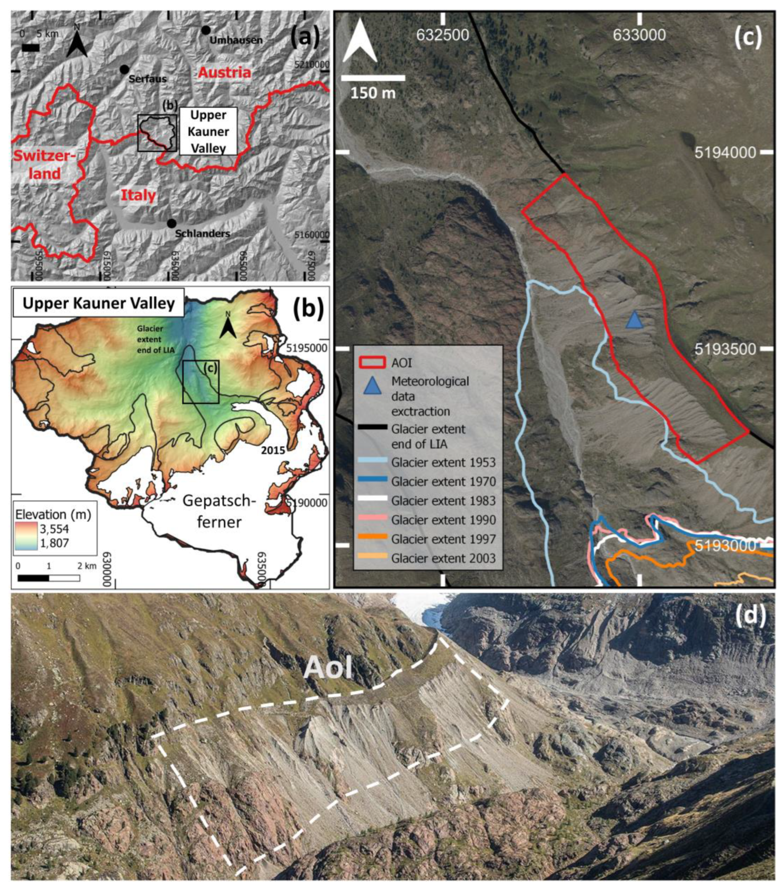
2. Study Area

The survey was conducted on a LIA lateral moraine in the proglacial area of the Gepatsch glacier (Gepatschferner) in the upper Kauner Valley (upper Kaunertal) in Tyrol, Austria, located in the Ötztal Alps, which is situated in the central Eastern Alps (Figure 1). Geologically, the Kauner Valley belongs to the Austroalpine crystalline complex, in which mainly crystalline rocks such as ortho- and paragneisses predominate [33,34,35]. Climatically, the valley is characterised by the Central Alpine dry region [36,37]. The valley is oriented north-south and borders Italy and the main Alpine ridge to the south. The maximum glacier extent at the end of the LIA was observed at the Gepatschferner in 1856 [38]. Apart from two glacier advances in 1920/21 and between 1977 and 1988 [38,39] the Gepatschferner has experienced continuous glacier retreat. Our Area of Interest (AoI, see Figure 1c,d, Table 1) is located in the upper part of an approximately 150 m high lateral moraine and is characterised by high morphodynamics and steep slope gradients. Typical moraine material both vegetated and nearly vegetation-free areas can be found.

3. Material and Methods

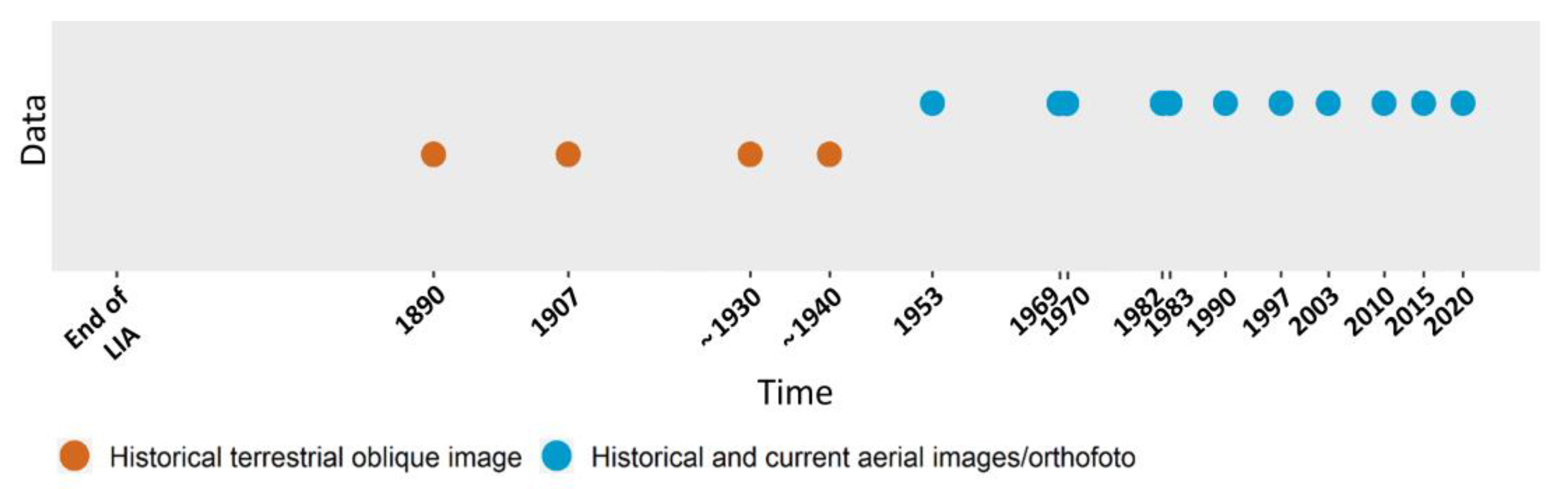
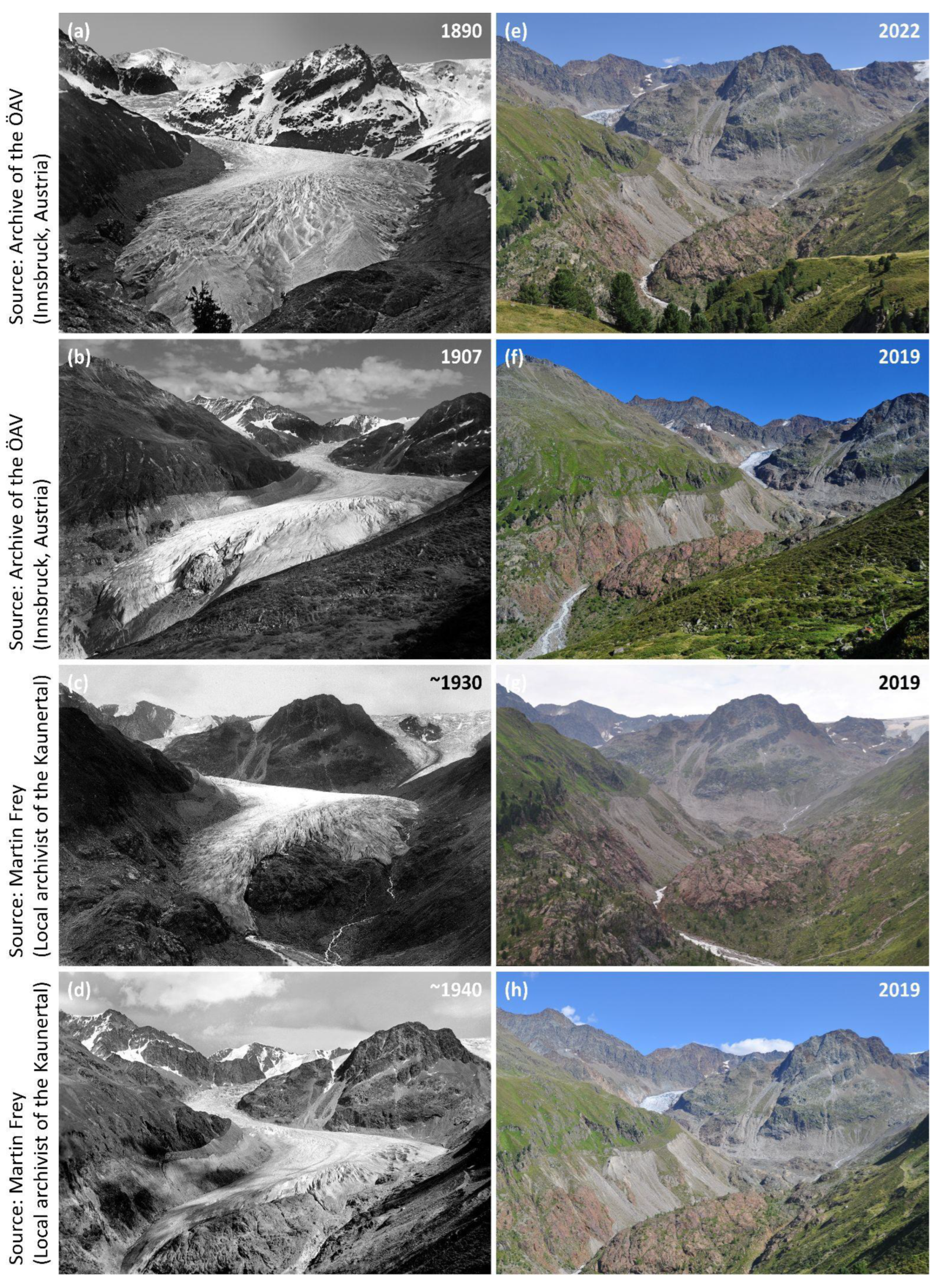
3.1. Photo Material

To enable the long-term observation of the development of the lateral moraine section, several terrestrial and aerial photographs were analysed. For the second half of the 19th century and the first half of the 20th century, historical terrestrial oblique photographs (Figure 2, Appendix B, Table A2) and from the second half of the 20th century onwards, aerial photographs were processed and analysed (Figure 2, Appendix A, Table A1).

3.2. Methods of Image Processing and Mapping

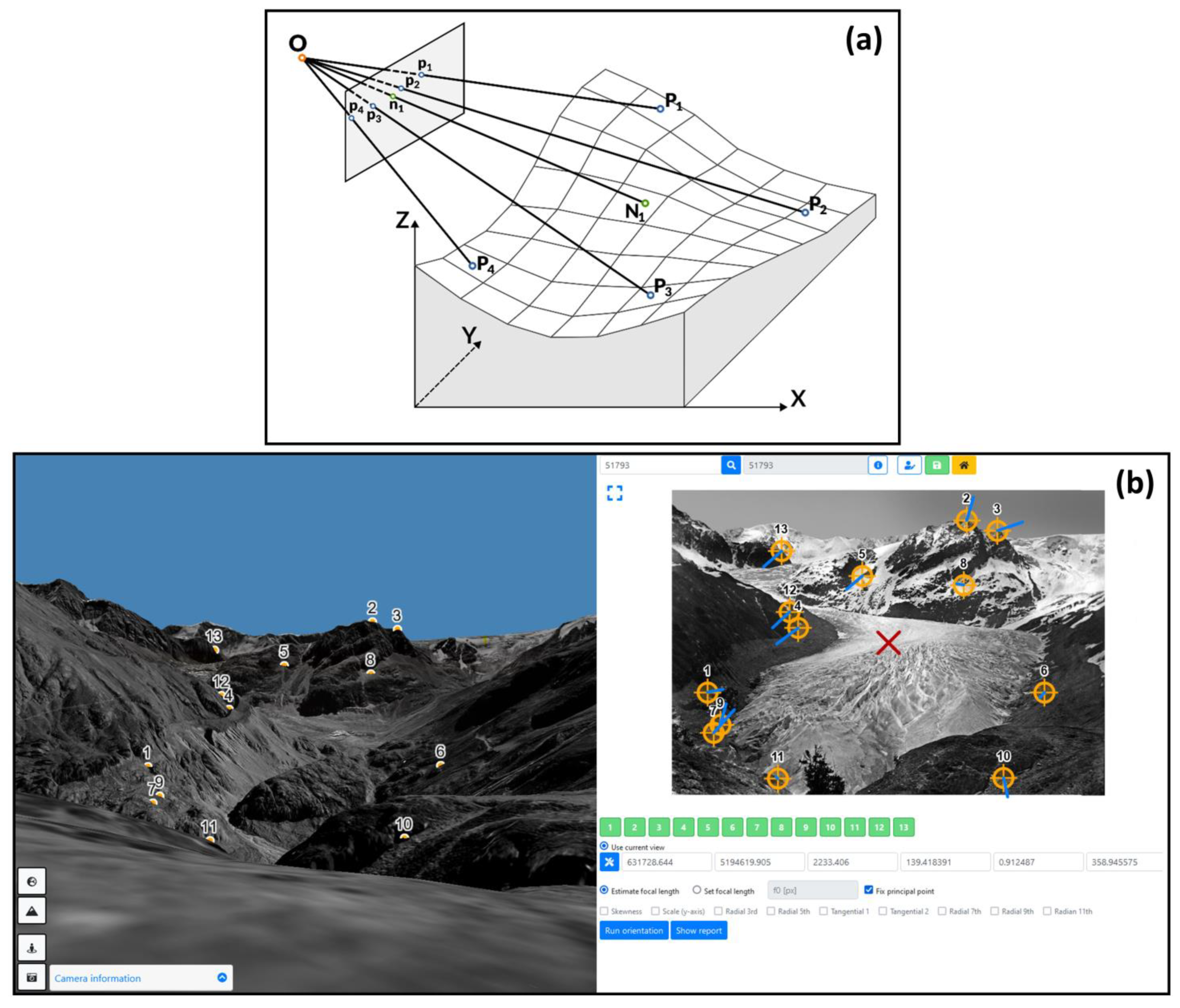
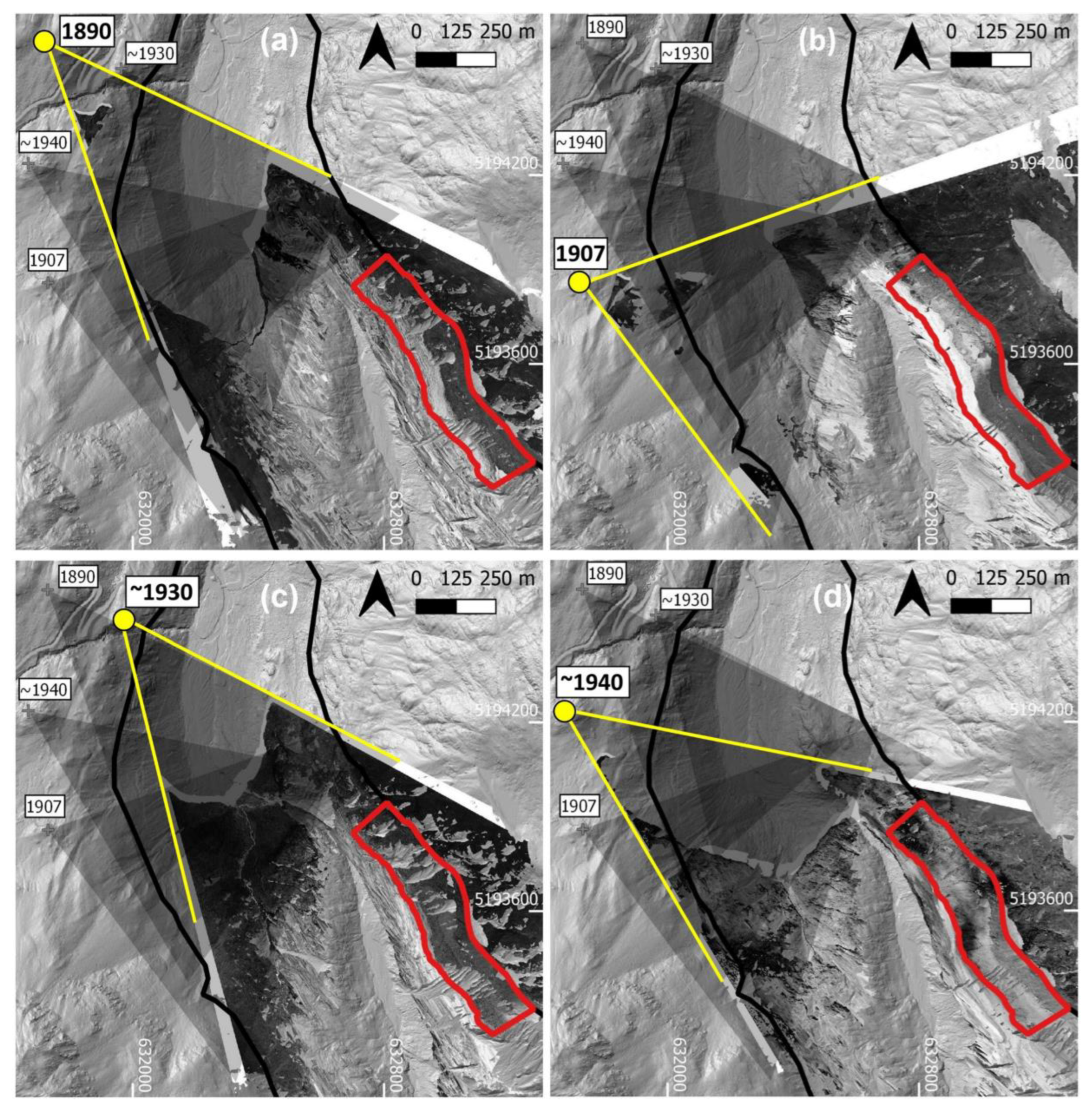
3.2.1. Processing of the Terrestrial Photos

In order to map the extent of the different surface types, mainly the morphodynamic area and land-cover types, within the AoI since 1890, a monoplotting tool was used [43]. With this tool the historical terrestrial photos from 1890, 1907, ~1930 and ~1940 (Figure 3; Appendix B, Table A2, Figure A1) were analysed. Using monoplotting, for each pixel of a photo the corresponding point in a (3D) global coordinate system is calculated by intersecting rays from the projection centre (O in Figure 3a) through each image pixel of the photo with a reference DTM (Figure 3a) [21,22,30].

Thus, each pixel of a photograph can be assigned a coordinate in a 3D object space [30]. Prior to monoplotting the interior (focal length f, coordinates of the principal point x0 and y0) and exterior orientation (coordinates of the projection centre and three rotation angles) of the camera have to be estimated as they are generally unknown for historical terrestrial photos [21]. For this purpose, approximately uniformly distributed ground control points (GCPs) were identified in each historical terrestrial oblique image as well as on the 1970 orthophoto with deposited 2017 DTM using a 3D viewer (Figure 3b; Appendix B, Table A3 and Table A4).

Then, both the interior and exterior orientation of each image were estimated using OrientAL [45]. Subsequently, the object coordinates of the image pixels corresponding to the outlines of the different surface types, mainly the morphodynamic area and land-cover types, were calculated by monoplotting using the estimated camera parameters and the reference DTM (2017, 1 m). The results from the orientation are shown in Figure 4 and Table 2. The coordinates of the principal point x₀ and y₀ were fixed in the image centre and only the remaining seven unknown camera parameters were estimated.

The calculated camera positions and orientations show that they were taken in the north-west direction of the AoI (Figure 4). The shortest distance to the AoI is 971 m (photo 1907), 1010 m (photo 1930), 1104 m (photo 1940) and 1242 m (photo 1890) metres respectively. In addition, Figure 4 shows the georeferenced orthophotos of the individual historical terrestrial photos.

3.2.2. Processing of the Aerial Photos

For quantitative mapping of the extent of different surface types, mainly the morphodynamic area and land-cover types, the area-wide and overlapping historical and current aerial photographs from the mid-20th century onwards (1953 to 2015) were processed into georeferenced orthophotos using Agisoft Metashape Professional (Version 1.6.6; Agisoft LLC, St. Petersburg, Russia) and Trimble Inpho (Version 9.2) for the 2003 aerial photo series. For a detailed description of the processing of the orthophotos we refer to [4,20,46,47]

3.3. Mapping of Morphodynamic and Land-Cover Types

In order to identify temporal and spatial changes within the AoI, morphodynamic and land-cover types were mapped using QGIS (version 3.16.7) [48] (Table 3). In morphodynamics, a classification was made between the (initial) gully system and the sediment accumulation at the glacier margin. In addition, geomorphological non-active areas (areas outside the gullies, which can mostly be considered as more stable) and glacier areas were mapped (lower part of the mapped glacier extent). Regarding the different land-cover types (Table 3) we mapped different land-cover types, but also the bedrock, and the glacier extent. The most abundant species for the land cover types scree slope, scree communities, alpine grassland and dwarf shrubs are listed in Table 3, which are based on vegetation surveys done in 2020. The mapping of the morphodynamic and land-cover types was carried out at intervals of 7–23 years, depending on the availability of photos (see Figure 2). If photo materials were temporally within 1–3 years, it was assumed that only very small changes in land-cover have occurred. In contrast to this, all photos were used for mapping the morphodynamics, as very short-term events can also occur. The analyses for showing the development over time were carried out in R (version 4.2.2) [49]. For further processing, all georeferenced shapefiles were converted into raster files with a resolution of 1 × 1 m. The rate of change in land-cover types over time on the whole AoI as well as the 1890 initial glaciated area, area with the initial gully system, and the more stable area respectively was displayed with alluvial diagrams using the packages tidyverse [50], raster [51], and ggalluvial [52,53].

The mapping was done manually through digitising the relevant objects of interest in the orthophotos, whether linear or areal and creating the corresponding spatially referenced vector datasets (line and polygon shapefiles) in QGIS (version 3.16.7) [48], which could then be exported. After that, the spatial and temporal extent of all surface types of the AoI was calculated. We compiled ten historical states of the AoI step-by-step going backwards in time to the first photograph. After one historical situation had been completed, we evaluated its relevance for the temporally younger situations and whether corrections would have to be made. Such a regressive-iterative approach allows for permanent critical revision of the reconstructed time segments already processed.

3.4. Generating Meteorological Data of the Study Area

Using simulated climate data generated by a regional climate model (RCM), the long-term air temperature (2 m above ground) as well as the precipitation of the AoI since the end of the LIA was determined. For the corresponding dynamic downscaling of climate data (from 1850 to 2015), the Advanced Research Version of the Weather Research and Forecasting (ARW-WRF) model (version 4.3) was used [54]. Therefore, the 20th Century Reanalysis version 3 (20CRv3) dataset was used as input [55,56,57]. To perform the simulations, the physical and dynamic options proposed by Collier and Mölg [58] were used (Appendix C, Table A5). In addition, the Noah land surface model, the Eta values of Collier et al. [59] and the 24 land use categories of the United States Geological Survey (USGS) were applied. Finally, simulated temperature data with a temporal and spatial resolution of one hour and two km respectively could be generated. For the subsequent period from 2016 to 2020, the ERA5 reanalysis dataset Hersbach et al. [60] was used, available with a temporal and spatial resolution of one hour and 55 × 55 km. The corresponding temperature data was extracted using the centre of the AoI (Figure 1). Additionally, an elevation correction of the temperature data was applied. The five years running mean of the average annual temperature and sum of summer (Mid-April to mid-October of each year) as well as winter precipitation (Mid-October to mid-April of each year) were used for the statistical analysis of the development of the land cover types.

3.5. Statistical Analysis of Land Cover Changes

For getting an information if there are other variables than the morphodynamic influencing the development of the land cover types on lateral moraines in the long-term, we performed a beta-regression using the package betareg [61] which is the suitable method for proportions. Therefore, the proportions have to be converted into values between zero and one using the formula

\frac{y * (n - 1) + 0.5}{n}

[62] where

y

is the proportion, and

n

the sample size. We used the variables age (years to the end of the observation period), amount of glacier per year (gla), the mean annual temperature (temp), the sum of summer (pre_sum) and winter precipitation (pre_win), and the amount of the more stable areas within the AoI (inact) for every year as independent variables. The equation for the different land cover types was the same and is shown in the following equation:

g (E [y^{t y p e}]) = β_{0} + β_{1} a g e + β_{2} g l a + β_{3} t e m p + β_{4} p r e_s u m + β_{5} p r e_w i n + β_{6} i n a c t + ε

where

g

(.) is the link function (logit link) and

E

[.] the expection;

y^{t y p e}

the transformed ratio of the land cover type following a beta distribution;

β_{0}

is the overall intercept, the

β_{s}

capture the effects, and

ε

is the remainder noise.

4. Results

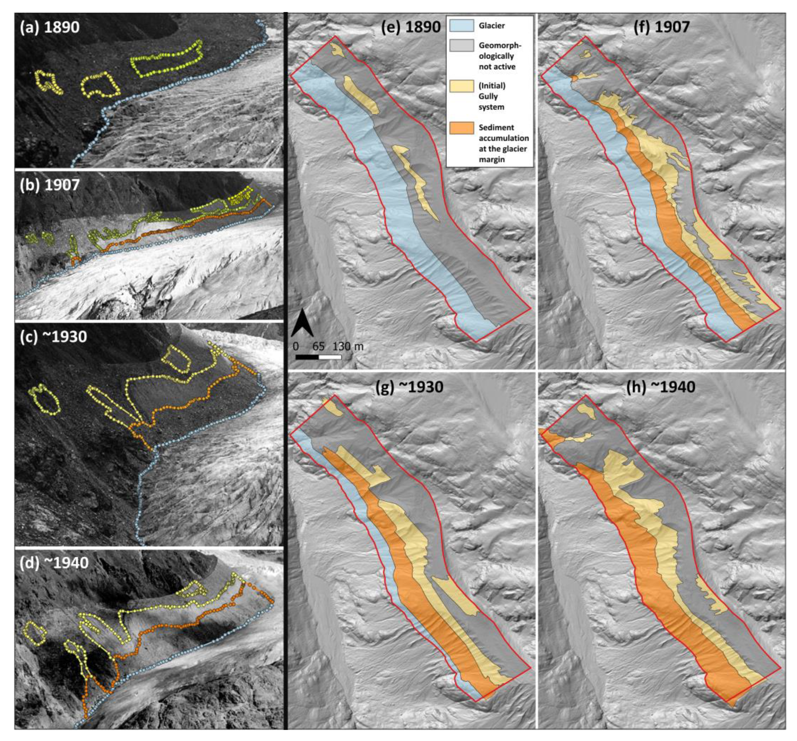
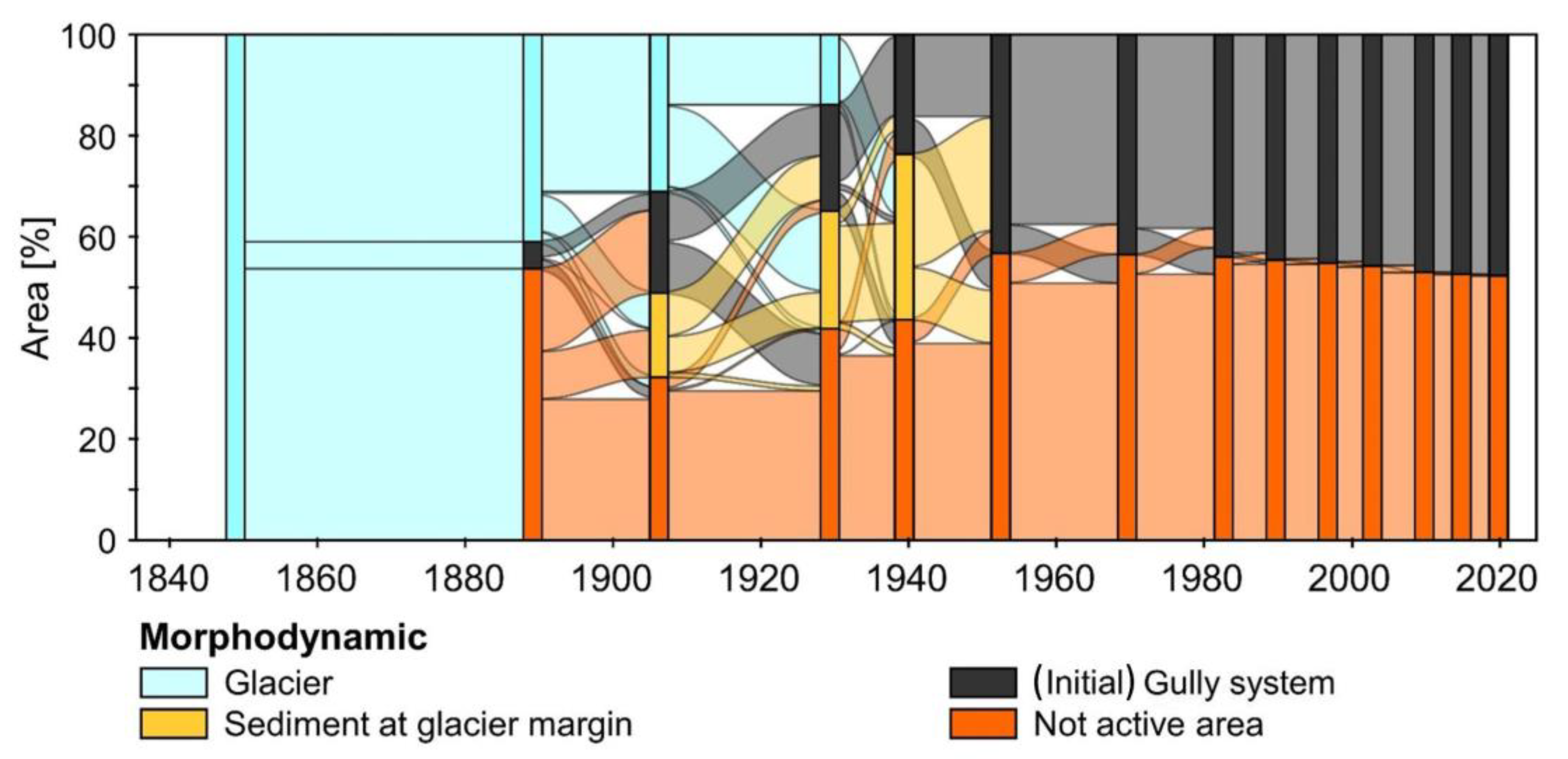
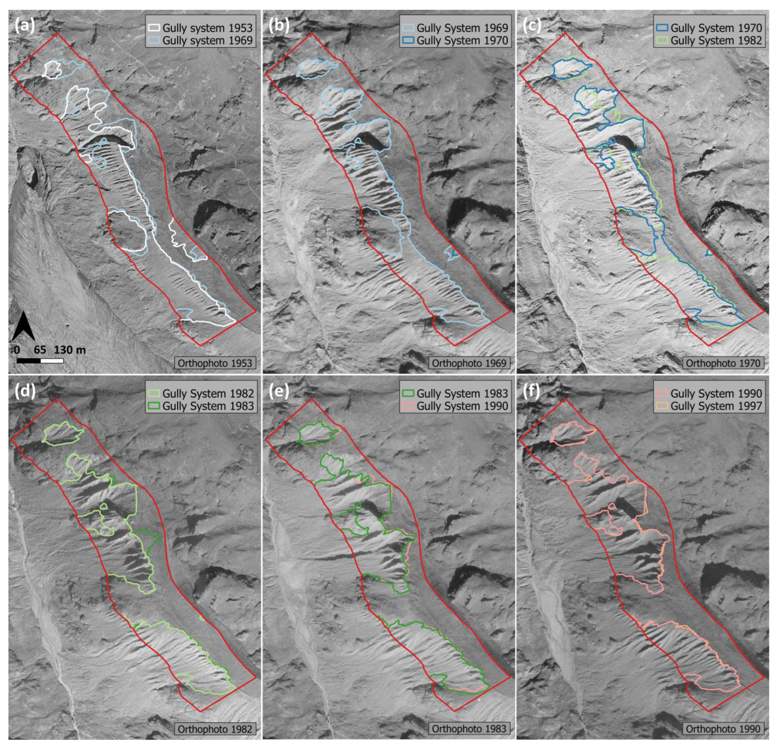
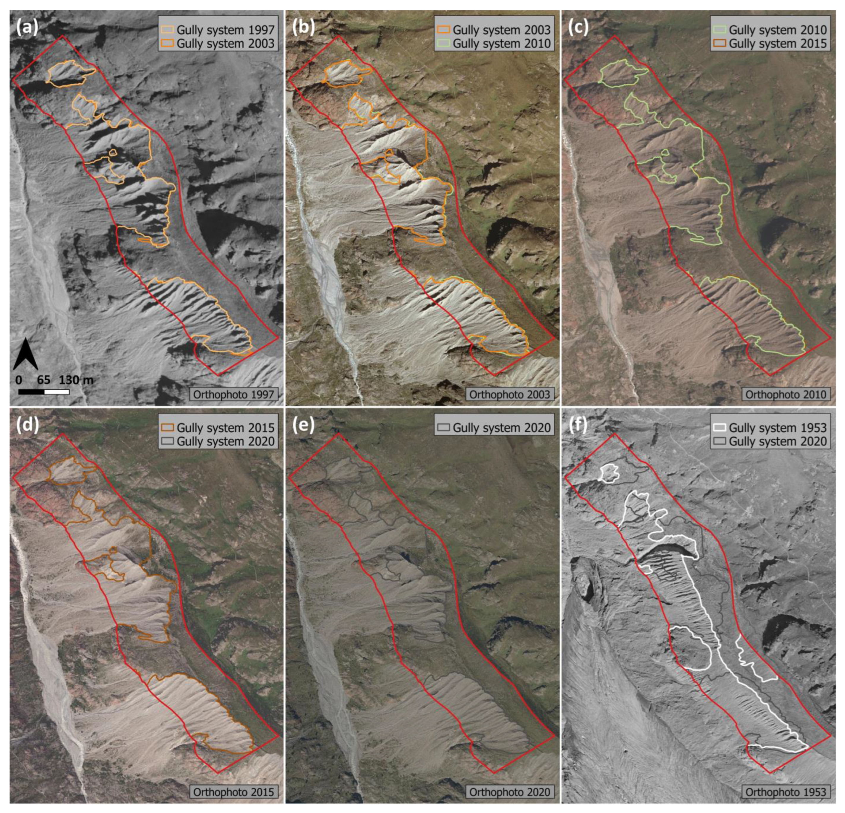
4.1. Long-Term Morphodynamic Development

While the AoI was fully glaciated at the end of the LIA, the glacier melted completely, over the years 1890, 1907, ~1930, by ~1940 (Figure 5 and 6; Appendix D, Table A6). From 1890 (5.1%) to 2020 (47.7%), there is an (almost) constant increase in the area of the (initial) gully system (Figure 5 and 6; Appendix D, Table A6; Appendix E, Figure A3 and Figure A4). However, between 1970 and 1982, there is a decrease (from 43.61% to 42.23% of the total AoI) in the extent of the mapped gully system (Appendix D, Table A6). Due to erosion processes, debris cones were formed at the glacier margin, which were visible from 1907 onwards and disappeared from the AoI by 1953 (Proportion of accumulated debris in 1907: 18.4%, ~1930: 23.9%, ~1940: 35%). The area defined as geomorphologically not active (more stable) is subject to greater variations. In the beginning (1890) with a high proportion (of 53.7%), this area expanded (almost) continuously until 1983 (60%) before it decreased again until 2020 (52.3%). In 2020, the gully system (47.7%) and the geomorphologically not active area (52.3%) had approximately the same share of area.

The initial gully system, already visible in 1890, had formed on the area exposed by the glacier until then (Figure 6). Between 1890 and 1953 the size of the (initial) gully system increased subsequently. These areas previously not detected as impacted by erosion, developed into gullies over time. Gullies were formed on previous area of the debris cone (sediment accumulation at the glacier margin) which was transported downslope on the melting glacier. Due to a strong headcut retreat, the size of the gully system increased (almost) continuously from 1953 to 2020, so that formerly geomorphologically not active areas became active. However, it is also evident that areas mapped as active gully system can certainly become stable again (throughout the investigation period) (Figure 6).

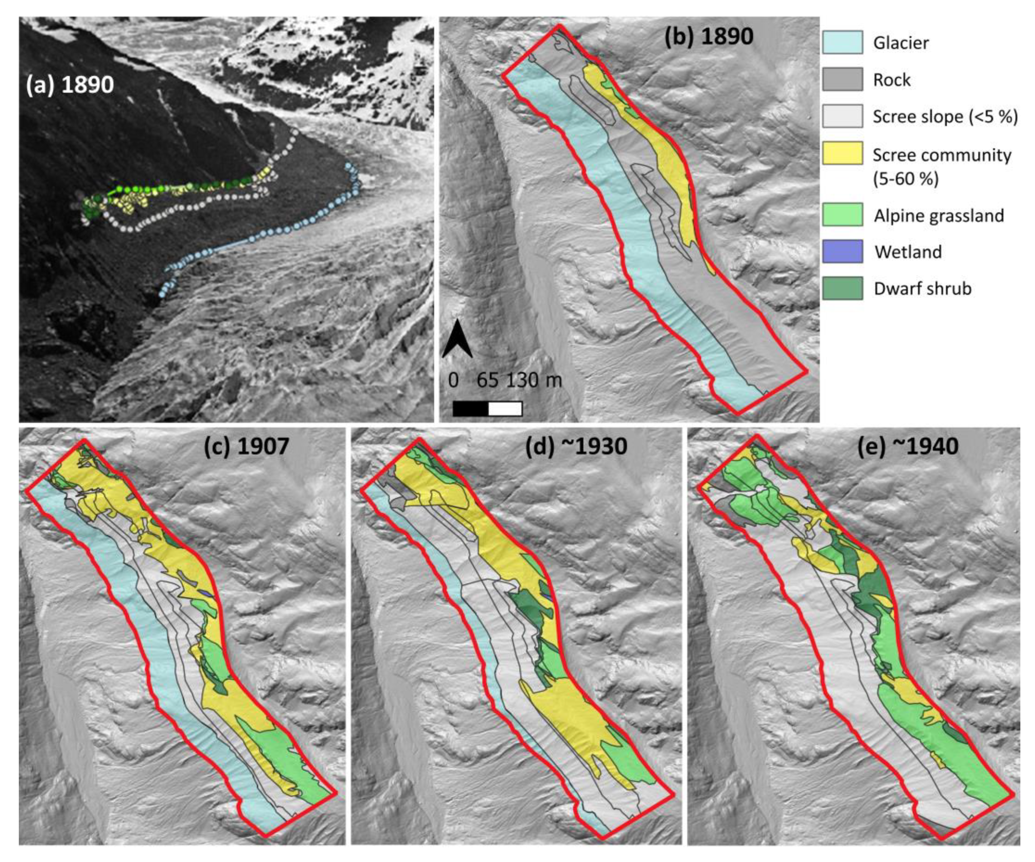
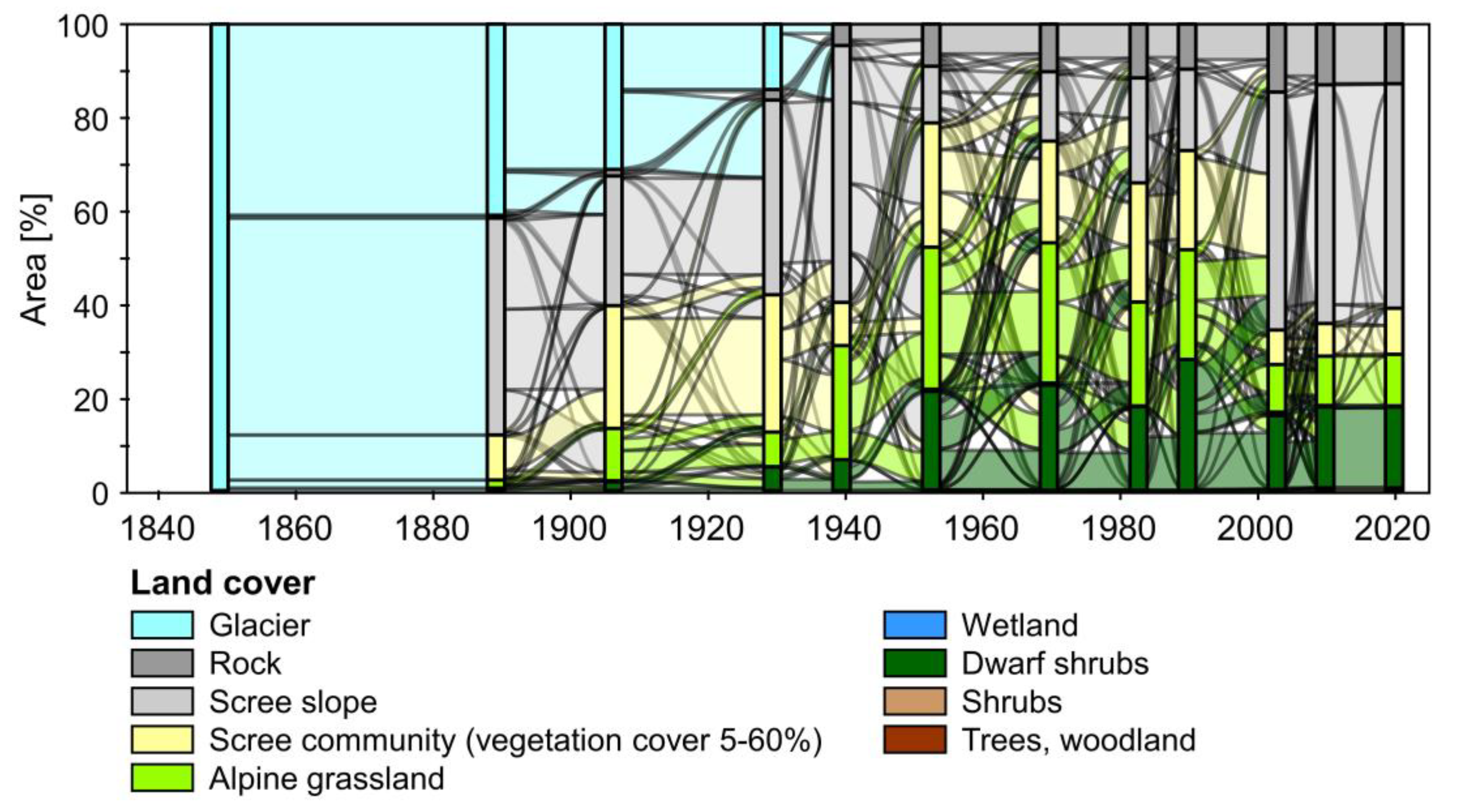
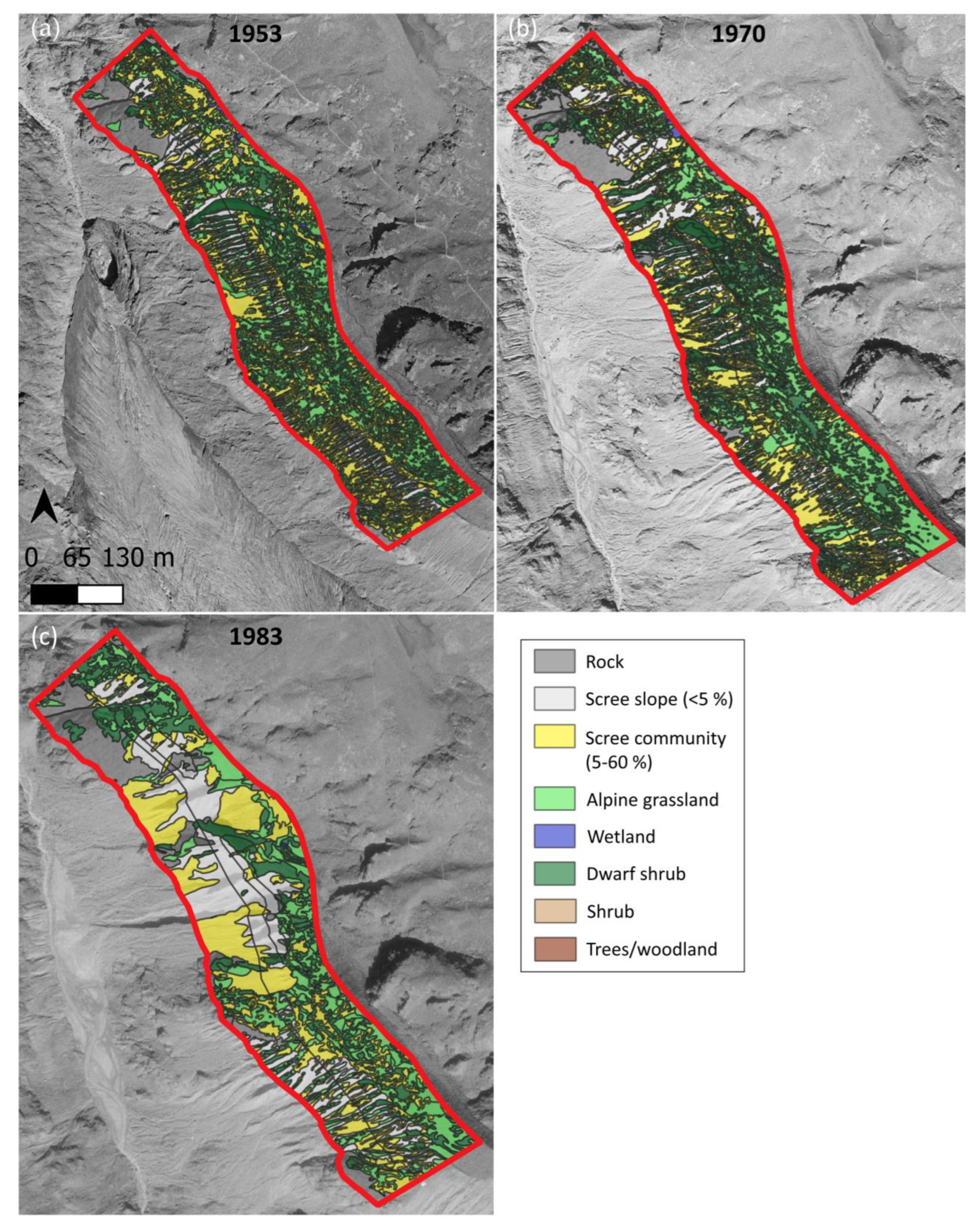
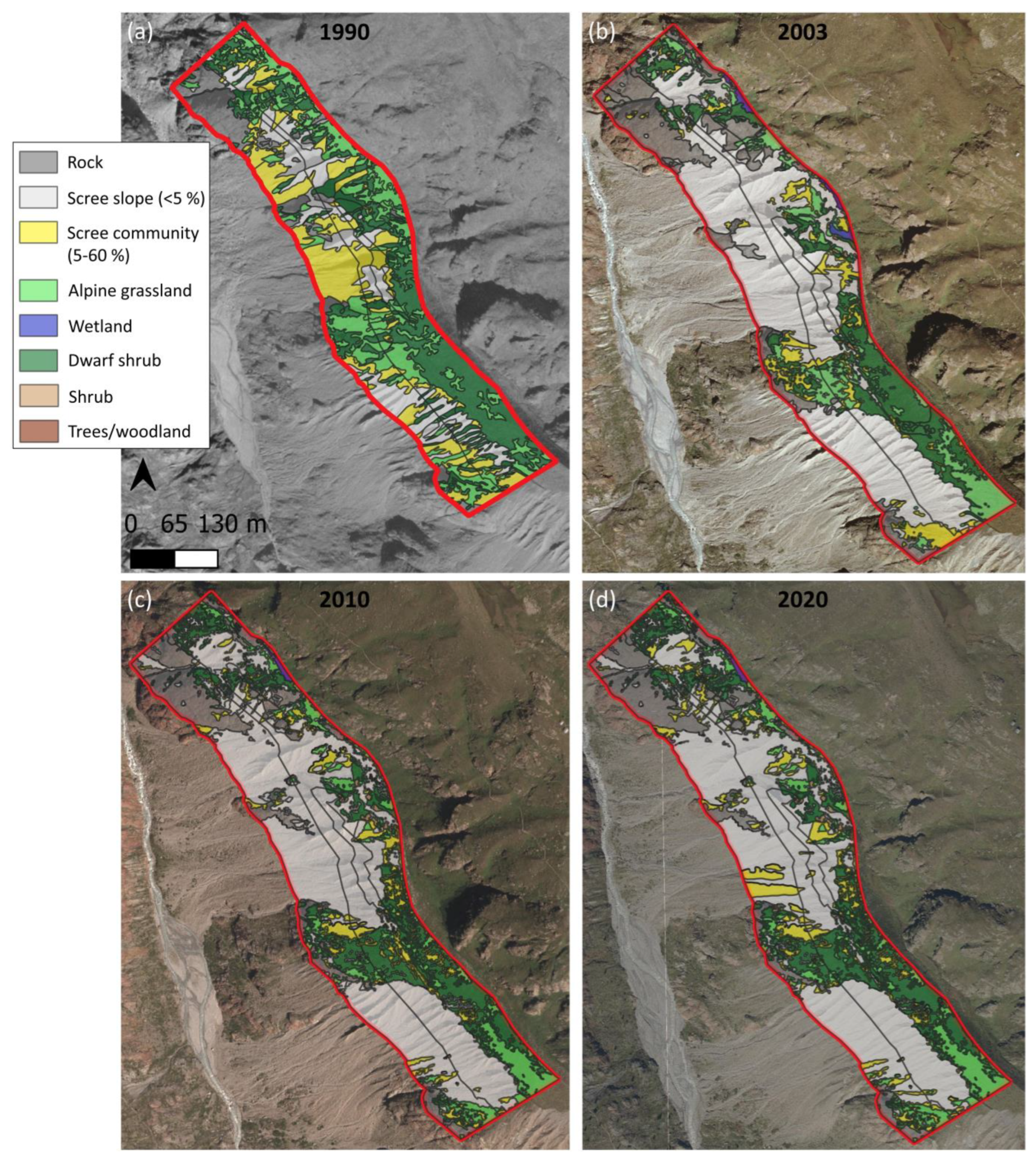
4.2. Long-Term Development of the Land-Cover Types

The entire AoI was covered by glaciers at the end of the LIA (Figure 7 and Figure 8 and Appendix D, Table A7). Until 1890 a small part was covered by bedrock (0.6%), the largest part by scree slope (46.5%), and further small parts to scree community with a low cover of vegetation (9.6%), alpine grassland (1.7%) and even dwarf shrubs (0.6%) (Figure 7 and Figure 8; Appendix D, Table A7). From ~1940 onwards, many of the scree slope stabilised and primary succession took place. As a result, the proportion of areas at the expense of scree slope communities, alpine grassland and dwarf shrubs increased to about 72.88% (Appendix E, Figure A5 and Figure A6). This share remained largely stable until 1990, but then there was another massive increase in scree slope. This indicates a renewed dynamic in these areas (Figure 8; Appendix D, Figure A2, Table A7 and Table A8). Mostly, these were alpine grasslands and scree communities that underwent a transition back into scree slopes. To a smaller extent, however, dwarf shrub communities were also affected (Figure 8; Appendix D, Figure A2, Table A7 and Table A8). The dispersal of wetlands, shrubs and trees/woodland started in 1953 and reached together until 2020 a proportion of 0.9% (Figure 8; Appendix D, Figure A2, Table A7 and Table A8; Appendix E, Figure A5 and Figure A6).

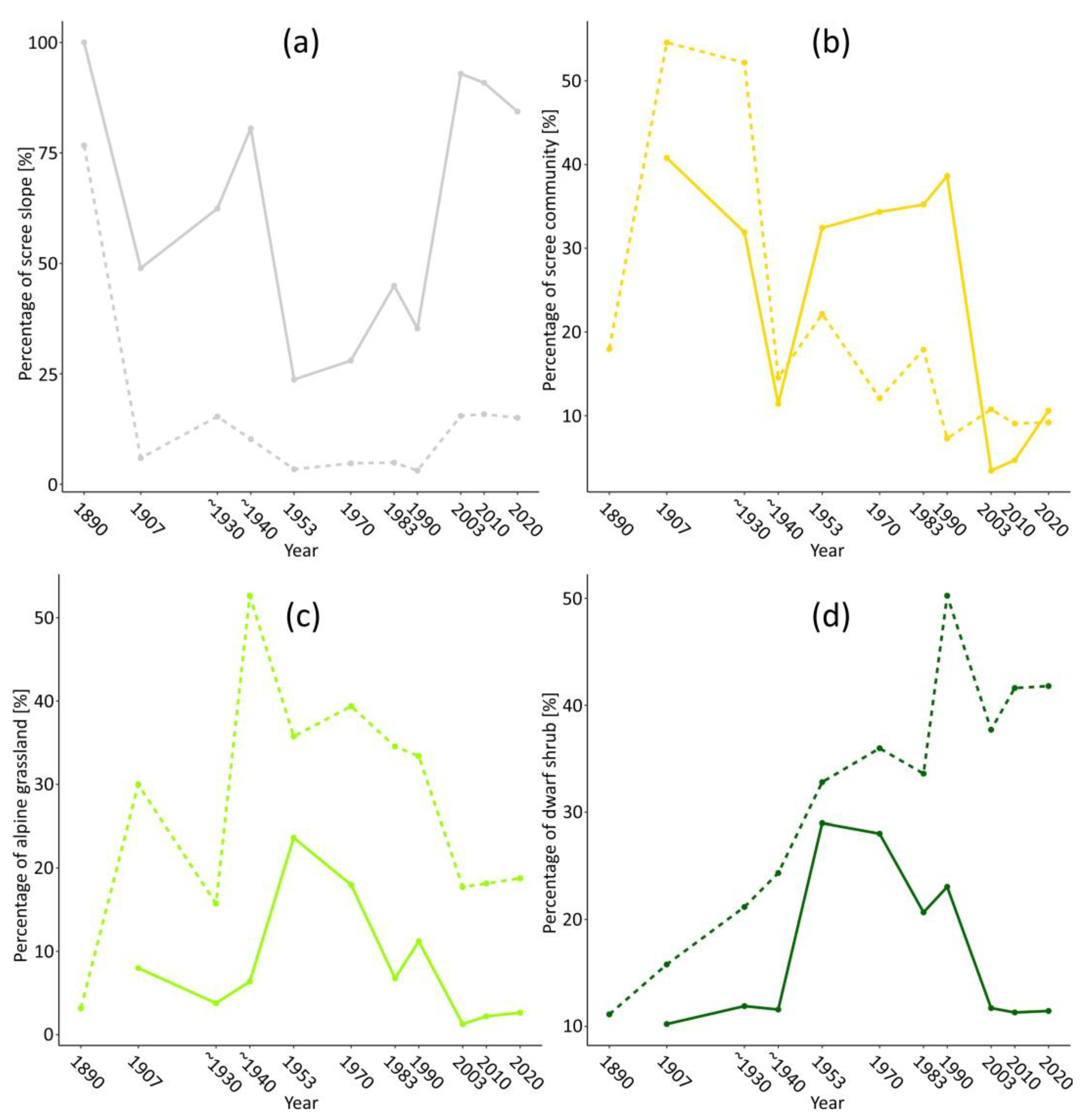
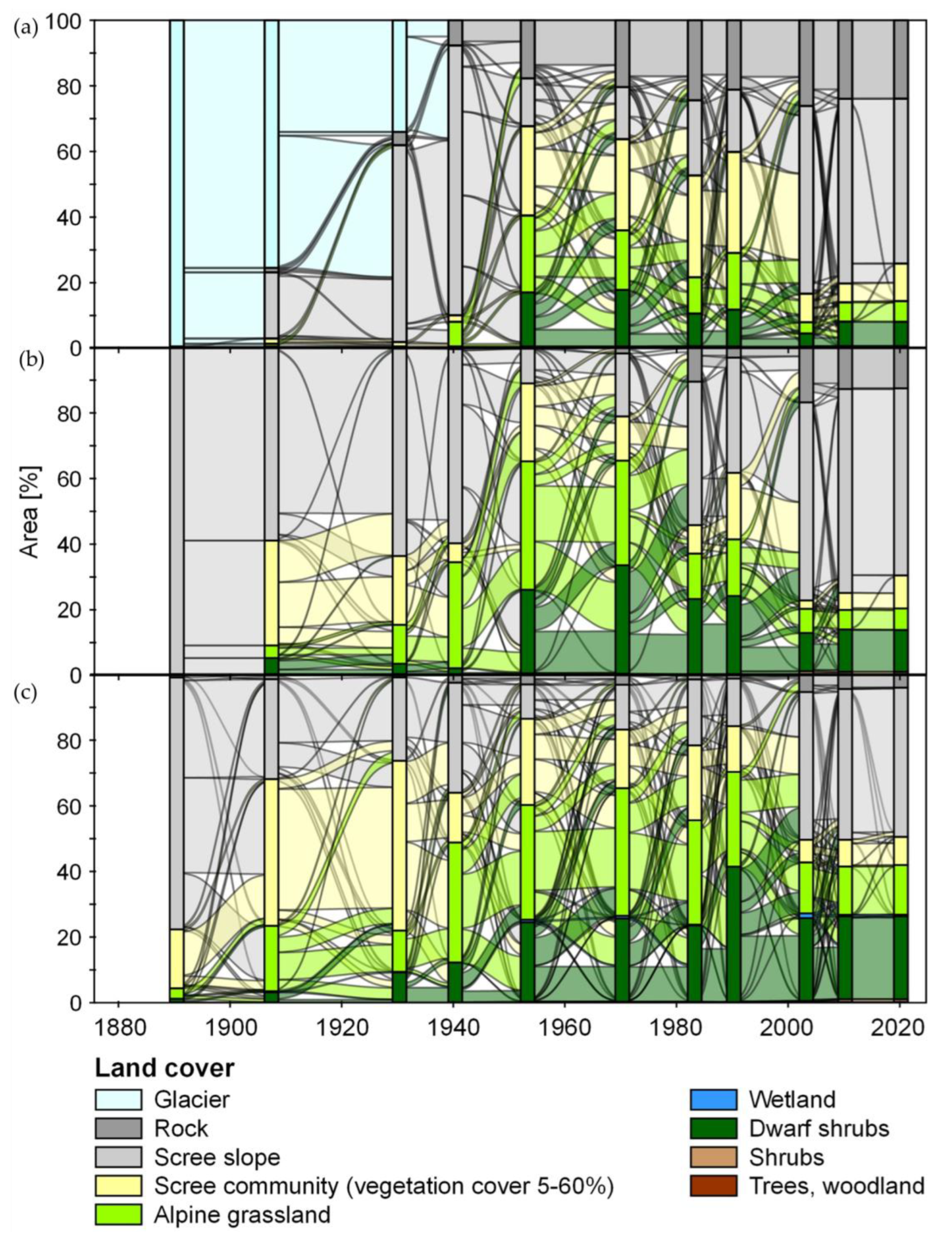
4.3. Development of Land-Cover Types in Geomorphologically Active and Not Active Areas

The development of the land-cover types within the gully systems as well as in the geomorphologically inactive (more stable) areas showed clear differences. The active gully systems were mainly characterised by scree slope (Figure 9a). However, due to the expansion of different vegetation types, these declined until 1953 (100 to 23.7%). After a strong decline from 1907 to 1940 (40.8 to 11.7%), mainly scree communities increased until 1990 (11.7 to 38.6%) (Figure 9b). Alpine grasslands and dwarf shrubs spread from 1907 (8%/0.2%) until 1953 (23.6%/19%) before declining again until 1990 (11.2%/13%) (Figure 9c,d). Between 1990 and 2003, a strong expansion of scree slope area (35.3% to 92.2%) is evident and a simultaneously strong decline of scree slope communities (38.6% to 3.5%), alpine grassland (11.2 to 1.3%) and dwarf shrubs (13 to 1.7%) (Figure 9c,d). Between 2003 and 2020, a slow increase in scree communities (3.5 to 10.6%) (Figure 9b) and alpine grassland (1.3 to 2.6%) (Figure 9c) can be observed, accompanied by a decline in scree slope areas (92.9 to 84.4%). Dwarf shrubs have remained at a similar level during this epoch (1.7 to 1.4%) (Figure 9d).

The geomorphologically non-active area (more stable) had clearly higher proportions of land-cover types, except scree slope (Figure 9a–d). Scree slope decreased strongly from 1890 (76.7%) to 1907 (5.9%) and, with some fluctuations, always remained below 20% until 2020 (Figure 9a). Scree communities increased clearly from 1890 to 1907 (18% to 54.6%) before decreasing strongly with fluctuations until 2020 (9.2%) (Figure 9b). Alpine grasslands also increased from 1890 to 1940 (from 3.2% to 52.6%) before also decreasing with variation by 2020 (18.8%) (Figure 9c). Dwarf shrubs increased almost continuously from 1890 to 2020 (from 1.1% to 31.8%), with the largest area in 1990 (40.2%) (Figure 9d).

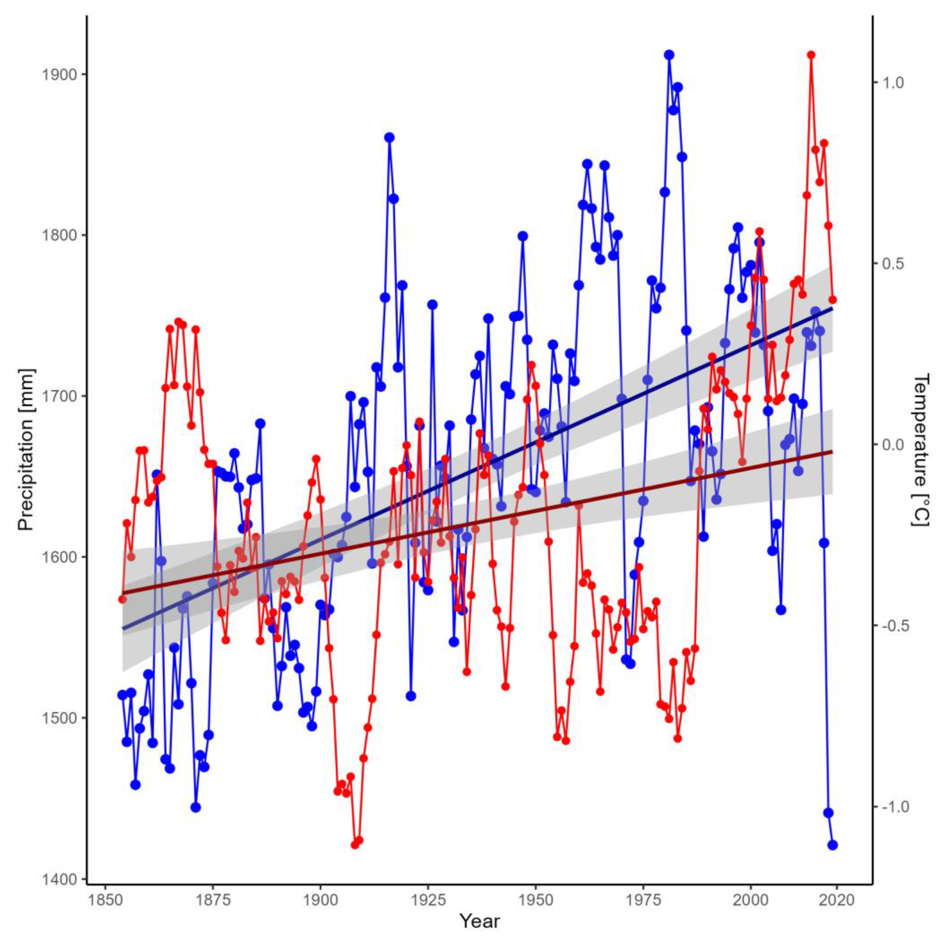
4.4. Land-Cover Change in Context with Morphodynamic and Meteorological Data

Figure 10 shows the running mean of the annual air temperature (2 m above ground) and the sums of the annual precipitation since 1850.

The analysis showed that the amount of glacier had only an impact on higher developed land-cover types. All analysed land-cover types except the dwarf shrubs were influenced by temperature. Summer and winter precipitation influenced the less developed land-cover types. The effect of age (years since observation) had a significant negative effect on scree slope (p = 0.038) and the amount of glacier per year was only significant for the land-cover types alpine grassland and dwarf shrub (p < 0.001 and p = 0.003, respectively) (Table 4). Temperature had a significant positive effect on scree slope (p < 0.001) and a significant negative effect on the land-cover types scree community (p = 0.002) alpine grassland (p = 0.006 (Table 4). Land cover types were also affected by summer precipitation with a significant negative effect on scree slope (p = 0.013) and a significant positive one on scree community (p = 0.041), respectively. Winter precipitation influenced scree slope significantly positive (p = 0.004) and scree community negative (p = 0.005) (Table 4). Concerning the morphodynamic more stable areas, we observed only a significant positive effect for dwarf shrubs (Table 4). The other three land-cover types were not significantly affected by the morphodynamic more stable areas. For the four analysed land-cover types the pseud R² was high (0.718, 0.728, 0.872, and 0.912, respectively). Also, the precision parameter (phi) was good for all four models (Table 4).

5. Discussion

5.1. Assessment of Technical Uncertainties and Errors

The accuracy and precision of the digital monoplotting results are influenced by several factors [21,22,23,24,25,26,28,29,30,31,32] including the distribution and number of the GCPs, the accuracy and precision of the DTM, the accuracy of the estimated camera parameters (interior and exterior orientation of the camera) and the angle of incidence between the image ray and the DTM. Furthermore, the quality of the historical terrestrial photos is not comparable to modern photos (e.g., lens distortion), further reduced by the way they were stored in the archives (e.g., stains, scratches), influencing the potentially achievable accuracy. When selecting the GCPs, we made sure to identify only terrain points in stable areas, further avoiding the highly dynamic proglacial area as much as possible, except for example rocky outcrops. Despite these restrictions, it was possible to identify more than 10 GCPs for each camera, distributed over the entire image. The use of a current (3D) object space (in this case the DTM 2017 (1 m)) and a historical terrestrial photo (from 1890 onwards) can also lead to errors in the mapping, as the mapping was carried out on the historical terrestrial photos, but the current surface might have changed considerably due to erosion processes such as landslides and debris flows [28,29]. This could be remedied by DTMs that are much closer in time to the historical terrestrial photos and thus possibly contain less changes in the surface topography, however, no corresponding DTM exists from this early period. Due to the strong surface changes on the AoI, especially due to the incision of the gullies, throughout the study period, there is strong shadowing of the georeferenced orthophotos based on the terrestrial photos, especially of the 1890 and ~1930 image (due to the low angle of incidence), as can be seen in Figure 5.

To estimate the spatial error of the GCPs, the corresponding theoretical 3D error was computed. This was calculated using the Euclidean distance between the user defined GCPs and the GCPs calculated by monoplotting. The determined error values of the GCPs show high variability. It ranges from minimum values of a few centimetres to maximum values of several tens of metres, although in extreme cases several hundred metres, or no value at all, could be reached, while the median of the GCPs of the four historical photos ranged from 3.5 to 17.5 m (Table 5/Appendix B, Table A3 and Table A4). The extreme cases occurred only at the top of hills or mountains where the calculated point was computed on the opposite slope or not at all (1890 photo: GCP numbers 2, 3 and 11 in Figure 3b and in Appendix B, Table A2 and ~1930 photo: GCP number 8 in Appendix B, Table A4).

The height above ground of the determined camera locations shows heights of 1.0 or 3.2 m, but also up to 12.3 and 13.7 m (Table 3), whereby the steep slopes of the location where the photos were taken play an important role, as a horizontal shift can quickly add up to a few metres in height. In any case, the determined coordinates of the camera locations mostly have an accuracy of a few decimetres to metres (up to a maximum of 7.3 m) (Table 3), which means that we consider the calculated camera locations to be acceptable. Bozzini et al. [21] show a theoretical 3D error of less than 10 m respectively less than 5 m for the prototype version of the WSL tool, if all basic requirements like a high image quality, a good distribution of control points, a DTM with high resolution and a good camera calibration are considered. Nevertheless, under optimal conditions, accuracies of less than one metre to decimetres are possible [22]. Conedera et al. [29,30] and Scapozza et al. [32] also report a possible spatial (3D) error of less than one metre (up to several metres) under optimal conditions, although even within the same photo higher errors can occur in flatter versus steeper areas due to the different angle of incidence.

Studies using photos from the Mountain Legacy Project [23,25] show clearly higher error values, but these studies used photos that cover larger and wider areas in high mountain regions (Rocky Mountains, Canada). Therefore, they are prone to higher error values (similar to the photos from the SEHAG project used in this study), as the accuracy decreases with increasing distance from the camera, due to the uncertainties in the orientation (angle). Stockdale et al. [23] show that especially the angle of incidence is of high importance, but that also the distance to the camera plays an important role, as it is difficult to set GCPs that have a very long distance, such as mountain peaks several kilometres away. In addition, we consider the angles of incidence in our study on the AoI to be high and therefore acceptable, due to the elevated position of the photo locations on the opposite slope and the steep slope of the lateral moraine itself. McCaffrey and Hopkinson [25] give a mean error vector length (between test points) of 23.9 m (range from 2 to 63.8 m) and a landscape level displacement of 7 m using seven photos. After removing two outliers, corresponding values of 16.5 m and 5.9 m were obtained, which are comparable to the values of Stockdale et al. [23] with 14.4 m and 2.9 m, respectively.

5.2. Opportunities and Limitations

While aerial photographs show an area-wide coverage of the surface, for terrestrial photographs, due to the oblique viewing geometry in combination with the complex topography especially in high mountain regions, some areas within the field of view cannot be observed due to occlusion [28]. We can confirm this, as the AoI is limited to a small area in the upper part of the lateral moraine. In the south-eastern part, the AoI is limited due to the curved topography of the lateral moraine, and in the north-western part, the AoI ends because rock exposures occurred on the slope (mainly in ~1930 and ~1940) and the mapping of the (initial) gully systems in several areas was not possible anymore due to the shadowing effect. While the upper boundary of the AoI was defined by the maximum glacier extent at the end of the LIA, the lower boundary was defined by the glacier extent in ~1940, so that a focus was placed on the erosion area in the upper part of the lateral moraine. This shows that although it is possible to map different surface types in high mountain regions using this approach, it can only be applied locally, and not over a wide area as with aerial photographs. While larger areas could be analysed with a greater number of historical terrestrial photos, these are usually available to a very limited extent and the identification of potential photos in the archives is time consuming. With very steep rock faces, however, aerial photos can reach their limits and the advantages of terrestrial photos can outweigh them, as due to the oblique geometry the angle of incidence is correspondingly higher [28]. Nevertheless, and most importantly, due to their temporal coverage into the 19th century, these photos provide a unique source for quantifying the change of different surface types in proglacial areas.

However, manual mapping is challenging and therefore prone to error. To minimise interpretation errors, only photos of good quality (e.g., photographic glass plates) and taken from a short distance from the AoI were selected, meaning that some photos that would have been available were not included in the analysis. Concerning the mapping of land-cover types, there exists a limitation by the quality of the photos and difficulties in mapping on black-white photos. Therefore, small errors of the mapping of the different land cover types may also be due to quality and difficulties in differentiation of the black-white photos and also by interpretation of the areas with shadow. By using a regressive-iterative approach the number of errors can be reduced as an unlikely sequence can be better detected. Due to the remote sensing data used (terrestrial photos and aerial photographs), it was not possible for us to identify individual species and to reconstruct them accordingly over the entire period. Nevertheless, based on field data collected in 2020, we can specialize the scree slope, scree community, alpine grassland, and dwarf shrub in more detail (Table 3).

5.3. Development of the Morphodynamic and Land-Cover Changes

The use of individual historical oblique photos by monoplotting has shown that it is possible to determine the changing extents of different surface types between the end of the LIA and the mid-20th century, thus quantifying to a certain point the approximately 100-year unknown initial response of surfaces to glacier retreat of proglacial areas, demonstrating the immense value of these photographs. By continuing the mapping using georeferenced orthophotos from the middle of the 20th century onwards and ensuring the compatibility of both mapping approaches, it was possible to continue this until 2020, covering a total period of 130 years. The results of the mapping of the upper lateral moraine section show a correspondingly high dynamic in recent decades. Also, for land-cover maps the development in the AoI was highly dynamic.

5.3.1. Morphodynamic Area

The mapping shows a continuous melting of the glacier from the end of LIA until ~1940. Although the visible glacier extents were mapped (and the lower surface determined as glacier), it must be assumed that the debris deposits on the glacier cover some parts of the glacier margin and thus the actual glacier extent is underestimated. However, this problem occurs in all terrestrial photographs (but mainly from 1907 to ~1940). This is evident in Figure 1, where the ~1940 (lower border of the AoI) and 1953 glacier extent overlap at two points, but the 1953 glacier extent is based on a DoD mapping (DEMs from 1970 and 1953) where volume changes were used to determine the full glacier extent even under debris deposits. Also, several studies show the occurrence of dead ice in this slope [4,5,20], at least until 1983 [20], which influenced the development of the erosion area for decades.

Although, an (almost) continuous increase in the area of the gully system within the AoI was observed from the end of LIA until 2020, several studies show a clear decrease in the corresponding erosion rate (based on quantitative volume data derived by DoDs) on the same slope, such as Altmann et al. [4] from the 1970s or Betz-Nutz et al. [5], Piermattei et al. [20] and Altmann et al. [6] from the 1950s onwards to present. However, between 1970 and 1982, there is a decrease in the extent of the gully system (Appendix D, Table A6), due to a part of an erosion area, previously (1971) mapped as geomorphologically active, which in turn were mapped in 1982 as bare rock and thus not geomorphologically active anymore (Appendix D, Table A6). Since several rocks were exposed over the entire period, this phenomenon occurs several times, but only predominates in the example mentioned. The geomorphologically inactive area was separated as well as possible from the (initial) gully system, although it cannot be excluded that some material was mobilised in the inactive area. Nevertheless, the (initial) gully system is well visible and was mapped due to its linear erosion form.

5.3.2. Land-Cover Types

The massive increase in scree slope between 1907 and 1930 was mainly caused by the release of new areas by the glacier (Appendix D Figure A2a). In 1953 we observed small flat areas within the gullies with alpine grassland or dwarf shrubs which eroded in the following periods. This can explain the high amount of dwarf shrubs and alpine grassland in 1953. The small flat areas with vegetation might be due to gliding down of whole areas with vegetation and erosion between vegetated areas. The detected large increase in alpine grassland, especially in the accumulation area might also be due to the glide down of larger parts in its entirety. The small flatter areas with denser vegetation eroded within the next periods. The clear decrease in higher developed land-cover types (mainly alpine grassland, and dwarf shrubs) as well as scree community and the accompanied increase in scree slope between 1990 and 2003 can be explained by the impact of geomorphic processes on the emergent and developing vegetation. For example the large-scale (wide area) erosion processes within the gully systems, as seen in a DoD of our AoI published by Piermattei et al. [20] between 1997 and 2003, have covered the upcoming vegetation. From 2003 (until 2020), a very slow increase in these land-cover types (scree community, alpine grassland and dwarf shrubs) can be observed again. The AoI experiences clearly less geomorphic activity during these epochs [20]. In the period 2010 to 2020 we could observe further stabilisation with mainly an evolvement from the scree slope to scree community and less changes for the other land-cover types.

There was nearly no comparable mapping for land-cover types found in literature, except the one by Hohensinner et al. [18]. However, in contrast to this study, they used historical maps for the long-term mapping rather than historical terrestrial photos, which, however, achieves a much lower spatial resolution. Using historical maps can cause problems in high elevations, especially above the timberline due to lower resolution and is therefore not appropriate for analysis on a small scale as these maps are often drawn at a coarser scale. The problems concerning scale, projection system, and reference points for elevation calculation as well as the precision during the field surveys and the accuracy are shown by Stäuble et al. [63].

Although morphodynamic activity highly influences land-cover development, the increase in alpine grassland and dwarf shrub might be due to the increasing temperature since the 1980s and faster change since 2011 as shown by Knoflach et al. [17], but it seems that the morphodynamic processes influence vegetation development more than the increasing temperature due to climate change. In contrast to Eichel et al. [14] we could only observe slope stabilisation when the morphodynamic activity already decreased.

6. Conclusions

To analyse quantitative landscape changes in the European Alps, mapping of different surface types, for example, can be carried out using georeferenced orthophotos based on aerial photos. However, the corresponding aerial photo series only extends up to about half of the 20th century, which limits the research design of many studies in time. Using digital monoplotting, it is possible to extend the time frame of mapping studies analysing landscape changes in high alpine geosystems using single terrestrial oblique photos by several decades into the late 19th and first half of the 20th century. By linking a single image to a 3D object space, quantitative analysis is possible by enabling real surface measurements of different image contents. Using several historical terrestrial oblique photographs from 1890 onwards (to ~1940) and georeferenced orthophotos based on aerial photos from 1953 to 2020, we show by mapping the quantitative changes of different surface types of a LIA lateral moraine section. The main conclusions of this study are listed below:

Using the monoplotting approach, it was possible to extend the temporal scope of a quantitative mapping study based on historical terrestrial oblique photographs within a proglacial area into the second half of the 19th century (1890), covering a total study period of over 130 years (1890–2020). This shows that the different orthophotos (based on terrestrial photos and aerial photographs) can be combined in a productive manner.
The (initial) gully systems expanded (almost) continuously since 1890 (respectively since the end of the LIA). However, several studies show that the erosion volume (mean annual erosion rate), between the 1950s/1970s and today, on the same slope is decreasing.
The vegetation covered areas show a clear increase within the AoI from 1890 (respectively since the end of the LIA) to 1953, as mainly scree communities (vegetation cover 5–60%), alpine grassland and dwarf shrubs expand. From 1953 to 2020, vegetation covered areas are clearly reduced as the scree expand again due to erosion processes. Especially in this epoch, rocks within the lateral moraine were also exposed. Land-cover types are clearly less developed in the active gully system than in the geomorphologically non-active areas, as erosion processes deplace or cover corresponding vegetated areas. The development of land-cover types is also significantly influenced by temperature and precipitation changes.
The approach of this study allows a better analysis of the paraglacial adjustment process, as in particular the early phase of the lateral moraine’s response to the ice loss can be determined and thus the initial gully formation as well as the development of the land-cover types can be detected, which previously remained unclear.

However, the digital monoplotting approach is highly dependent on the availability, number and quality of the corresponding historical oblique photos, and shadowing effects in high alpine regions can quickly lead to corresponding limits. Nevertheless, the study shows the enormous potential of these photos. Therefore, we encourage scientists to conduct further long-term studies using digital monoplotting with terrestrial historical oblique photos to better reconstruct corresponding climate change consequences in high alpine geosystems.

Author Contributions

Conceptualization, M.A., K.R., F.H., E.T. and M.B.; methodology, M.A., S.M.-F., K.R., M.P., J.R., F.F., T.H. (Toni Himmelstoß), F.H., T.H. (Tobias Heckmann), N.P., C.R., E.T. and M.B.; software, M.A., S.M.-F., K.R., M.P., N.P. and C.R.; formal analysis, M.A., K.R. and M.P.; investigation, M.A., K.R. and M.P.; data curation, M.A., K.R. and M.P.; writing—original draft preparation, M.A. and K.R.; writing—review and editing, M.A., S.M.-F., K.R., M.P., J.R., F.F., F.H., T.H. (Toni Himmelstoß) and E.T.; visualization, M.A., K.R., M.P. and E.T.; supervision, F.H., E.T., N.P. and M.B.; project administration, F.H., T.H. (Tobias Heckmann), E.T. and M.B; funding acquisition, F.H., T.H. (Tobias Heckmann), E.T. and M.B. All authors have read and agreed to the published version of the manuscript.

Funding

The study was part of the SEHAG project (“SEnsitivity of High Alpine Geosystems to climate change since 1850”) and financially supported by the German Research Foundation (DFG) project number 3,942,00609, the Austrian Science Fund (FWF) and the Autonomous Province of Bozen/Bolzano, South Tyrol (Grant numbers: BE 1118/38-1, BE 1118/39-1, BE 1118/40-1, HA 5740/10-1, HE 5747/6-1, ER 905/1-1, MA 6966/4-1, LA 4426/1-1, 4062-N29 and IT-DFG 781,607).

Data Availability Statement

Aerial photos have been provided by the Federal Office of Metrology and Surveying of Austria, Vienna (BEV) and the Department of Geoinformation of the Province of Tyrol (Innsbruck, Austria). The orthophoto 2020 was downloaded from the Department of Geoinformation of the Province of Tyrol (TIRIS maps, https://tiris.maps.arcgis.com/home/index.html, accessed on 2 May 2022). The historical oblique photos have been made available by the archive of the German and Austrian Alpine Club (1890 und 1907) as well as by Martin Frey (~1930 und ~1940), a local chronicler in the Kauner Valley. The DEM 2017, which is based on airborne LiDAR data, comes from an own field campaign of the Chair of Physical Geography of the University of Eichstätt-Ingolstadt. The meteorological data were generated within the SEHAG project (“Sensitivity of High Alpine Geosystems to Climate Change since 1850”). The data can be requested from the authors.

Acknowledgments

We would like to thank the German Research Foundation (DFG), the Austrian Science Fund (FWF), and the Autonomous Province of Bozen/Bolzano, South Tyrol for their financial support. We would also like to thank the Federal Office of Metrology and Surveying (BEV, Vienna, Austria) and the Department of Geoinformation of the Province of Tyrol (Innsbruck, Austria) for providing the aerial photographs. Furthermore, we would like to thank the Archive of the German Alpine Club and Martin Frey, a local chronicler of the Kaunertal, for providing the historical terrestrial oblique photos of the Gepatsch glacier.

Conflicts of Interest

The authors declare no conflict of interest. The funders had no role in the design of the study; in the collection, analyses, or interpretation of data; in the writing of the manuscript; or in the decision to publish the results.

Appendix A

Table A1. Attributes of historical and current aerial photos.

Year of Recording	Source/ Purpose and Designation	Photos ¹	Camera Model, Band	Focal Length [mm]	Flying Altitude [m a.s.l.]	Type/Scanning Resolution [μm]	Result	Resolution Orthophoto [m]
5 June/31 August and 8 September 1953 ²	BEV/Forest condition estimation, C	124	Wild RC5, BW	210.1	ca. 3330	film/15	Orthophoto	0.23
7 October 1969	BEV/Austrian Glacier Overall Survey	23	Wild RC5/RC8, BW	152.0	ca. 3450	film/15	Orthophoto	0.5
29 September 1970	Land Tirol/Overall flight Tyrol	26	Wild RC5/RC8	210.4	ca. 8665	film/12	Orthophoto	0.2
18 August 1971	Land Tirol/Overall flight Tyrol	91	Wild RC5/RC8, BW	209.5	ca. 3080	film/12	Orthophoto	0.2
14 September 1982	BEV/High Flight Tyrol/80	34	Wild RC10, BW	152.6	ca. 6090	film/15	Orthophoto	0.5
24 September 1983	BEV/Kaunertal	7	Wild RC10, BW	152.6	ca. 4840	film/15	Orthophoto	0.4
10 October 1990	BEV/KF 171–173	35	Wild RC10, BW	152.6	ca. 5850	film/15	Orthophoto	0.53
11 September 1997	BEV/KF 173	25	Wild RC10, BW	152.7	ca. 6010	film/15	Orthophoto	0.55
5 September 2003	BEV/Ötztaler Alpen/Oberinntal	59	N/A, RGB	305.1	ca. 4800	film/15	Orthophoto	0.35
31 July 2010	Land Tirol/Reutte-Sölden	413	N/A, RGBN	---	ca. 2870	digital	Orthophoto	0.2
5 October 2015	Land Tirol/Landeck	94	UltraCamX, RGBN	---	ca. 3250	digital	Orthophoto	0.4
8 September 2020 ³	Land Tirol/ Landeck	N/A	N/A, N/A	---	N/A	digital	Orthophoto	0.2

¹ Photos were used to process the entire catchment of the upper Kaunertal, ² Data set were processed into one orthophoto, ³ the Province of Tyrol (Office of the Provincial Government of Tyrol/Department of Geoinformation) provided the orthophoto as download (https://www.tirol.gv.at/sicherheit/geoinformation/geodaten/orthophotos/, accessed on 2 May 2022).

Appendix B

Table A2. Attributes of historical terrestrial oblique photos.

Year of Recording	Photographer	Source	Image Medium	Type	Colour	Width and Height [pixel, cm]	Resolution [dpi]	Image Depth [BIT]
1890	N/A	Archive of the ÖAV (Innsbruck, Austria)	Negative glass plate	Digitised	B&W	4607 × 307, 19.5 × 13	600	24
1907	N/A	Archive of the ÖAV (Innsbruck, Austria)	Negative glass plate	Digitised	B&W	4607 × 307, 19.5 × 13	600	24
~1930 (estimated)	N/A	Martin Frey (Local archivist of the Kaunertal)	N/A	Digitised	B&W	9213 × 614, 19.5 × 13	1200	8
~1940 (estimated)	N/A	Martin Frey (Local archivist of the Kaunertal)	N/A	Digitised	B&W	8976 × 614, 19.5 × 13	1200	8

Table A3. Monoplotting accuracy of 1890 and 1907 photos: Coordinates of the user defined GCPs (East, North and Height), by monoplotting calculated GCPs (East monoplotting, North monoplotting and Height monoplotting) and corresponding Euclidean distance as error value (Delta 3D). In two cases, no coordinates could be determined using monoplotting. Used coordinate system: ETRS89/UTM Zone 32N coordinate system (EPSG code: 25832).

Historical Terrestrial Image	GCP Number	East [m]	North [m]	Height [m]	East Monoplotting [m]	North Monoplotting [m]	Height Monoplotting [m]	Delta 3D [m]
1890	1	632,685.9	5,194,046.4	2153.5	632,683.9	5,194,044.5	2154.1	2.8
	2	633,755.7	5,191,665.6	3034.7	-	-	-	-
	3	633,620.1	5,191,552.4	2981.4	-	-	-	-
	4	633,228.3	5,193,382.3	2312.4	633,167.3	5,193,441.0	2303.8	85.1
	5	634,099.5	5,192,196.0	2682.9	634,097.6	5,192,210.5	2673.2	17.5
	6	632,267.2	5,193,552.0	2160.9	632,266.8	5,193,555.0	2159.9	3.1
	7	632,554.6	5,194,113.3	2096.5	632,567.4	5,194,101.5	2097.8	17.5
	8	633,537.9	5,191,990.8	2606.3	633,541.6	5,191,992.0	2607.1	4.0
	9	632,583.6	5,194,081.1	2104.3	632,588.8	5,194,077.0	2106.9	7.1
	10	631,871.4	5,194,377.8	2176.2	631,870.9	5,194,378.5	2175.4	1.1
	11	631,771.5	5,194,586.7	2221.7	632,450.3	5,194,062.0	2036.3	877.7
	12	633,316.5	5,193,349.7	2371.0	633,286.8	5,193,380.5	2362.6	43.7
	13	635,653.5	5,191,577.7	3079.1	635,650.3	5,191,598.5	3062.5	26.8
1907	1	633,903.8	5,191,802.8	3001.5	633,898.3	5,191,800.5	2996.7	7.7
	2	633,788.7	5,191,703.1	3038.4	633,782.3	5,191,696.0	3033.9	10.6
	3	635,966.8	5,192,804.1	3319.8	635,962.1	5,192,808.0	3308.6	12.8
	4	636,185.9	5,192,836.2	3513.2	636,171.9	5,192,847.5	3495.6	25.1
	5	632,880.3	5,193,919.6	2285.5	632,878.6	5,193,920.0	2283.3	2.8
	6	633,178.7	5,193,634.4	2351.9	633,176.8	5,193,635.5	2350.6	2.6
	7	632,468.7	5,193,780.7	2075.9	632,471.6	5,193,780.0	2078.3	3.8
	8	635,078.2	5,192,954.0	2797.6	635,078.6	5,192,958.5	2795.6	5.0
	9	633,600.1	5,192,238.7	2516.7	633,610.6	5,192,234.0	2524.3	13.8
	10	634,146.5	5,192,466.7	2554.4	634,156.1	5,192,466.0	2559.9	11.1
	11	631,784.8	5,193,797.0	2252.2	631,785.0	5,193,797.0	2252.2	0.2
	12	633,152.3	5,193,425.2	2309.2	633,212.1	5,193,408.5	2314.2	62.3

Table A4. Monoplotting accuracy of ~1930 and ~1940 photos: Coordinates of the user defined GCPs (East, North and Height), by monoplotting calculated GCPs (East monoplotting, North monoplotting and Height monoplotting) and corresponding Euclidean distance as error value (Delta 3D). In two cases, no coordinates could be determined using monoplotting. Used coordinate system: ETRS89/UTM Zone 32N coordinate system (EPSG code: 25832).

Historical Terrestrial Image	GCP Number	East [m]	North [m]	Height [m]	East Monoplotting [m]	North Monoplotting [m]	Height Monoplotting [m]	Delta 3D [m]
~1930	1	632,555.5	5,194,112.2	2096.4	632,552.9	5,194,114.5	2095.2	3.8
	2	632,594.4	5,194,061.4	2108.8	632,594.6	5,194,061.0	2108.8	0.5
	3	633,263.0	5,193,341.0	2327.6	633,252.7	5,193,351.0	2323.6	14.9
	4	632,279.4	5,193,591.3	2136.4	632,279.9	5,193,590.0	2136.4	1.4
	5	633,775.0	5,191,663.0	3040.9	633,772.8	5,191,664.5	3039.1	3.2
	6	632,502.6	5,193,815.5	2074.7	632,501.0	5,193,815.5	2073.4	2.1
	7	632,460.0	5,194,170.6	2072.8	632,460.6	5,194,170.5	2072.6	0.7
	8	636,614.9	5,190,978.5	3546.9	-	-	-	-
	9	632,432.6	5,193,770.2	2050.1	632,432.6	5,193,770.0	2050.3	0.3
	10	633,259.8	5,192,088.3	2412.6	633,251.1	5,192,106.0	2399.5	23.7
	11	633,628.1	5,191,548.1	2986.9	633,625.8	5,191,557.5	2979.1	12.4
	12	633,272.8	5,193,521.1	2400.0	633,272.2	5,193,516.5	2402.6	5.3
	13	633,820.9	5,192,338.5	2502.0	633,804.7	5,192,349.0	2491.6	22.0
~1940	1	632,544.0	5,193,660.3	2126.0	632,542.9	5,193,664.5	2125.4	4.4
	2	633,207.9	5,193,569.0	2363.0	633,207.6	5,193,567.5	2362.8	1.6
	3	636,190.2	5,192,839.9	3516.1	636,189.6	5,192,840.0	3516.8	0.9
	4	633,563.4	5,191,691.1	2790.6	633,563.2	5,191,678.5	2799.6	15.5
	5	632,299.4	5,193,577.7	2142.1	632,298.3	5,193,576.0	2142.4	2.1
	6	633,535.3	5,191,986.0	2607.7	633,533.6	5,191,999.0	2600.8	14.8
	7	633,665.8	5,193,738.3	2565.9	633,663.6	5,193,733.5	2567.9	5.6
	8	633,151.3	5,193,427.7	2309.2	633,147.5	5,193,432.5	2307.7	6.3
	9	633,327.3	5,193,333.1	2382.1	633,325.4	5,193,341.0	2378.7	8.8
	10	632,325.2	5,193,633.5	2105.9	632,325.8	5,193,633.0	2106.0	0.8
	11	633,904.9	5,191,943.1	2873.0	633,907.3	5,191,941.0	2875.3	3.9
	12	632,456.5	5,193,736.9	2073.9	632,456.7	5,193,735.0	2074.4	2.0

Figure A1. Historical terrestrial photos (a–d) and the correspondingly reproduced photos from the same location between 2019 and 2022 (e–h).

Appendix C

Table A5. Summary of the WRF configuration.

Domain Configuration
Horizontal grid spacing	18-, 6-, 2-km (D1, D2 and D3)
Grid dimensions	190 × 190, 151 × 142, 121 × 139
Lateral boundary condition	variable (20CRv3 at 1° × 1°, 3-h)
Time step	90, 30, 10 s
Vertical levels	50
Model top pressure	10 hPa
Model physics
Microphysics	Morrison [64]
Cumulus	Kain-Fritsch (none in D3) [65]
Radiation	RRTMG [66]
Planetary boundary layer	Yonsei State University [67]
Atmospheric surface layer	Monin Obukhov [68]
Land surface	Noah [69]
Dynamics
Top boundary conditions	Rayleigh damping
Diffusion	Calculated in physical space

Appendix D

Table A6. Changes of surface types/morphodynamic area from End of LIA to 2020 with the proportion [%].

Surface Type/Morphodynamic Area	End of LIA	1890	1907	~1930	~1940	1953	1969	1970
(Initial) Gully system	0	5.13	22.71	23.82	26.82	43.34	43.49	43.61
Geomorphological not active area	0	53.71	28.30	39.12	38.21	56.66	56.51	56.39
Sediment accumulation at the glacier margin	0	0	18.40	23.85	34.97	0	0	0
Glacier	100	41.16	30.59	13.21	0	0	0	0
Surface Type/Morphodynamic Area	1982	1983	1990	1997	2003	2010	2015	2020
(Initial) Gully system	42.23	44.05	44.62	45.24	45.77	47.04	47.43	47.70
Geomorphological not active area	57.77	59.95	55.38	54.76	54.23	52.96	52.57	52.30
Sediment accumulation at the glacier margin	0	0	0	0	0	0	0	0
Glacier	0	0	0	0	0	0	0	0

Table A7. Changes of land cover types from End of LIA to 2020 with the proportion of each land-cover type in the area of interest (AoI).

Land-Cover Type	1850	1890	1907	~1930	~1940	1953	1970	1983	1990	2003	2010	2020
Glacier	100.0	40.98	31.10	14.02	0.00	0.00	0.00	0.00	0.00	0.00	0.00	0.00
Rock	0.00	0.56	1.42	2.23	4.57	8.98	10.21	11.50	9.62	14.57	12.97	12.74
Scree slope	0.00	46.52	27.79	41.76	55.09	12.19	14.88	22.54	17.46	50.95	51.15	48.14
Scree community	0.00	9.63	26.34	29.45	9.27	26.61	21.79	25.53	21.28	7.42	7.01	9.87
Alpine grassland	0.00	1.70	11.25	7.36	24.45	30.50	30.05	22.30	23.49	10.19	10.64	11.07
Wetland	0.00	0.00	0.20	0.12	0.00	0.42	0.45	0.12	0.00	0.77	0.27	0.27
Dwarf shrub	0.00	0.60	1.91	5.06	6.62	21.16	22.51	17.90	28.11	15.81	17.35	17.31
Shrub	0.00	0.00	0.00	0.00	0.00	0.08	0.07	0.00	0.01	0.25	0.53	0.53
Trees, woodland	0.00	0.00	0.00	0.00	0.00	0.06	0.05	0.11	0.04	0.04	0.08	0.08

Table A8. Changes of land-cover types from End of LIA to 2020 with the proportion [%], on the 1890 initially glaciered area (upper part), on the 1890 initially morphodynamic active area (initial gully system) (middle part), and on the initially more stable (not active) area (lower part).

1890 initially glaciered area
Land-Cover Type	1890	1907	~1930	~1940	1953	1970	1983	1990	2003	2010	2020
Glacier	100.0	75.89	34.22	0.00	0.00	0.00	0.00	0.00	0.00	0.00	0.00
Rock	0.00	1.35	4.05	7.72	17.80	20.49	24.51	21.26	26.26	24.07	24.03
Scree slope	0.00	20.27	60.34	82.70	14.66	15.93	23.05	19.11	57.55	56.60	50.55
Scree community	0.00	1.63	1.39	2.01	27.38	27.99	31.19	30.95	8.74	5.76	11.49
Alpine grassland	0.00	0.86	0.00	7.57	23.59	18.22	11.13	17.37	3.44	5.92	6.36
Wetland	0.00	0.00	0.00	0.00	0.00	0.00	0.00	0.00	0.00	0.00	0.00
Dwarf shrub	0.00	0.00	0.00	0.00	16.57	17.37	10.04	11.31	4.00	7.51	7.44
Shrub	0.00	0.00	0.00	0.00	0.01	0.00	0.00	0.00	0.00	0.08	0.08
Trees, woodland	0.00	0.00	0.00	0.00	0.00	0.00	0.07	0.00	0.01	0.06	0.06
1890 initially morphodynamic active area (initial gully system)
Land-Cover Type	1890	1907	~1930	~1940	1953	1970	1983	1990	2003	2010	2020
Glacier	0.00	0.00	0.00	0.00	0.00	0.00	0.00	0.00	0.00	0.00	0.00
Rock	0.00	0.34	0.48	0.65	0.53	1.98	10.63	3.26	16.94	12.84	12.64
Scree slope	100.0	58.84	63.42	59.37	10.62	19.24	48.83	35.21	60.54	62.35	57.19
Scree community	0.00	32.06	21.04	5.80	23.85	13.52	8.69	20.34	2.57	5.18	10.11
Alpine grassland	0.00	3.85	11.89	32.41	39.23	31.98	13.89	17.33	7.39	5.98	6.57
Wetland	0.00	0.00	0.00	0.00	0.00	0.00	0.00	0.00	0.00	0.00	0.00
Dwarf shrub	0.00	4.91	3.18	1.78	25.50	33.12	22.95	23.86	11.65	12.91	12.75
Shrub	0.00	0.00	0.00	0.00	0.22	0.15	0.00	0.00	0.91	0.74	0.74
Trees, woodland	0.00	0.00	0.00	0.00	0.06	0.00	0.00	0.00	0.00	0.00	0.00
1890 initially more stable (not active) area
Land-Cover Type	1890	1907	~1930	~1940	1953	1970	1983	1990	2003	2010	2020
Glacier	0.00	0.00	0.00	0.00	0.00	0.00	0.00	0.00	0.00	0.00	0.00
Rock	1.05	1.58	1.02	2.57	3.10	3.20	1.65	1.39	5.42	4.49	4.10
Scree slope	76.70	30.36	25.35	33.54	10.48	13.67	20.02	14.42	45.01	45.96	45.47
Scree community	17.95	44.72	51.75	15.17	26.27	17.86	22.84	13.97	6.90	8.16	8.61
Alpine grassland	3.18	19.92	12.54	36.56	34.95	38.89	31.81	28.85	15.57	14.71	15.13
Wetland	0.00	0.37	0.22	0.00	0.79	0.85	0.22	0.00	1.42	0.49	0.49
Dwarf shrub	1.12	3.04	9.12	12.16	24.20	25.34	23.31	41.28	25.23	25.23	25.23
Shrub	0.00	0.00	0.00	0.00	0.12	0.12	0.00	0.02	0.37	0.86	0.86
Trees, woodland	0.00	0.00	0.00	0.00	0.10	0.08	0.15	0.07	0.07	0.11	0.11

Figure A2. Changes of the land-cover types on in 1890 (a) initial glaciated area, (b) the initial active area (initial gully system), and (c) the initial more stable (not active) area; the different colours indicate the different land-cover types.

Appendix E

Figure A3. Continued mapping of the different surface types (morphodynamic mapping) using georeferenced orthophotos based on overlapping area-wide aerial photographs from 1953 to 1990 (a–f). The red line indicates the area of interest.

Figure A4. Continued mapping of the different surface types (morphodynamic mapping) using georeferenced orthophotos based on overlapping area-wide aerial photographs from 1997 to 2020 (a–f). The red line indicates the area of interest.

Figure A5. Continued mapping of the different surface types (land-cover mapping) using georeferenced orthophotos based on overlapping area-wide aerial photographs from 1953 to 1983 (a–c). The red line indicates area of interest (AoI).

Figure A6. Continued mapping of the different surface types (land-cover mapping) using georeferenced orthophotos based on overlapping area-wide aerial photographs from 1990 to 2020 (a–d). The red line indicates the area of interest.

References

Heckmann, T.; Morche, D. Geomorphology of Proglacial Systems: Landform and Sediment Dynamics in Recently Deglaciated Alpine Landscapes; Springer: Cham, Switzerland, 2019; ISBN 9783319941820. [Google Scholar]
Hock, R.; Rasul, G.; Adler, C.; Cáceres, B.; Gruber, S.; Hirabayashi, Y.; Jackson, M.; Kääb, A.; Kang, S.; Kutuzov, S.; et al. High Mountain Areas. In IPCC Special Report on the Ocean and Cryosphere in a Changing Climate; Pörtner, H.-O., Roberts, D.C., Masson-Delmotte, V., Zhai, P., Tignor, M., Poloczanska, E., Mintenbeck, K., Alegría, A., Nicolai, M., Okem, A., et al., Eds.; Cambridge University Press: Cambridge, UK; New York, NY, USA, 2019; pp. 131–202. [Google Scholar] [CrossRef]
Deline, P.; Gruber, S.; Delaloye, R.; Fischer, L.; Geertsema, M.; Giardino, M.; Hasler, A.; Kirkbride, M.; Krautblatter, M.; Magnin, F.; et al. Chapter 15—Ice Loss and Slope Stability in High-Mountain Regions. In Snow and Ice-Related Hazards, Risks, and Disasters; Haeberli, W., Whiteman, C., Shroder, J.F., Eds.; Academic Press: Cambridge, MA, USA, 2015; pp. 521–561. [Google Scholar] [CrossRef]
Altmann, M.; Piermattei, L.; Haas, F.; Heckmann, T.; Fleischer, F.; Rom, J.; Betz-Nutz, S.; Knoflach, B.; Müller, S.; Ramskogler, K.; et al. Long-Term Changes of Morphodynamics on Little Ice Age Lateral Moraines and the Resulting Sediment Transfer into Mountain Streams in the Upper Kauner Valley, Austria. Water 2020, 12, 3375. [Google Scholar] [CrossRef]
Betz-Nutz, S.; Heckmann, T.; Haas, F.; Becht, M. Development of the morphodynamics on LIA lateral moraines in ten glacier forefields of the Eastern Alps since the 1950s. Earth Surf. Dynam. Discuss. 2022; in review. [Google Scholar] [CrossRef]
Altmann, M.; Pfeiffer, M.; Haas, F.; Rom, J.; Fleischer, F.; Heckmann, T.; Piermattei, L.; Wimmer, M.; Braun, L.; Stark, M.; et al. Long-term monitoring (1953–2019) of geomorphologically active sections on LIA lateral moraines under changing meteorological conditions. EGUsphere 2023. [Google Scholar] [CrossRef]
Ballantyne, C.K. A general model of paraglacial landscape response. Holocene 2002, 12, 371–376. [Google Scholar] [CrossRef]
Ballantyne, C.K. Paraglacial geomorphology. Quat. Sci. Rev. 2002, 21, 1935–2017. [Google Scholar] [CrossRef]
Curry, A.M.; Cleasby, V.; Zukowskyj, P. Paraglacial response of steep, sediment-mantled slopes to post-‘Little Ice Age’ glacier recession in the central Swiss Alps. J. Quat. Sci. 2006, 21, 211–225. [Google Scholar] [CrossRef]
Ballantyne, C.K.; Benn, D.I. Paraglacial Slope Adjustment and Resedlmenfation following Recent Glacier Retreat, Fåbergstølsdalen, Norway. Arct. Alp. Res. 1994, 26, 255–269. [Google Scholar] [CrossRef]
Ballantyne, C.K.; Benn, D.I. Paraglacial slope adjustment during recent deglaciation and its implications for slope evolution in formerly glaciated environments. In Advances in Hillslope Processes; Anderson, M.G., Brooks, S.M., Eds.; Wiley: Chichester, UK, 1996; Volume 2, pp. 1173–1195. [Google Scholar]
Curry, A.M.; Ballantyne, C.K. Paraglacial modification of glacigenic sediment. Geogr. Ann. Ser. A Phys. Geogr. 1999, 81, 409–419. [Google Scholar] [CrossRef]
Eichel, J.; Corenblit, D.; Dikau, R. Conditions for feedbacks between geomorphic and vegetation dynamics on lateral moraine slopes: A biogeomorphic feedback window. Earth Surf. Process. Landf. 2016, 41, 406–419. [Google Scholar] [CrossRef]
Eichel, J.; Draebing, D.; Meyer, N. From active to stable: Paraglacial transition of Alpine lateral moraine slopes. Land Degrad. Dev. 2018, 29, 4158–4172. [Google Scholar] [CrossRef]
Gurnell, A.M.; Corenblit, D.; García de Jalón, D.; Del González Tánago, M.; Grabowski, R.C.; O’Hare, M.T.; Szewczyk, M. A Conceptual Model of Vegetation-hydrogeomorphology Interactions Within River Corridors. River Res. Appl. 2016, 32, 142–163. [Google Scholar] [CrossRef]
Haselberger, S.; Ohler, L.-M.; Junker, R.R.; Otto, J.-C.; Glade, T.; Kraushaar, S. Quantification of biogeomorphic interactions between small-scale sediment transport and primary vegetation succession on proglacial slopes of the Gepatschferner, Austria. Earth Surf. Process. Landf. 2021, 46, 1941–1952. [Google Scholar] [CrossRef]
Knoflach, B.; Ramskogler, K.; Talluto, M.; Hofmeister, F.; Haas, F.; Heckmann, T.; Pfeiffer, M.; Piermattei, L.; Ressl, C.; Wimmer, M.H.; et al. Modelling of Vegetation Dynamics from Satellite Time Series to Determine Proglacial Primary Succession in the Course of Global Warming—A Case Study in the Upper Martell Valley (Eastern Italian Alps). Remote Sens. 2021, 13, 4450. [Google Scholar] [CrossRef]
Hohensinner, S.; Atzler, U.; Fischer, A.; Schwaizer, G.; Helfricht, K. Tracing the Long-Term Evolution of Land Cover in an Alpine Valley 1820–2015 in the Light of Climate, Glacier and Land Use Changes. Front. Environ. Sci. 2021, 9, 683397. [Google Scholar] [CrossRef]
Schiefer, E.; Gilbert, R. Reconstructing morphometric change in a proglacial landscape using historical aerial photography and automated DEM generation. Geomorphology 2007, 88, 167–178. [Google Scholar] [CrossRef]
Piermattei, L.; Heckmann, T.; Betz-Nutz, S.; Altmann, M.; Rom, J.; Fleischer, F.; Stark, M.; Haas, F.; Ressl, C.; Wimmer, M.; et al. Evolution of an Alpine proglacial river during seven decades of deglaciation quantified from photogrammetric and LiDAR digital elevation models. Earth Surf. Dynam. Discuss. 2022. [Google Scholar] [CrossRef]
Bozzini, C.; Conedera, M.; Krebs, P. A new tool for obtaining cartographic georeferenced data from single oblique photos. In Proceedings of the XXIIIrd International CIPA Symposium, Prague, Czech Republic, 12–16 September 2011. [Google Scholar]
Bozzini, C.; Conedera, M.; Krebs, P. A New Monoplotting Tool to Extract Georeferenced Vector Data and Orthorectified Raster Data from Oblique Non-Metric Photographs. Int. J. Herit. Digit. Era 2012, 1, 499–518. [Google Scholar] [CrossRef]
Stockdale, C.-A.; Bozzini, C.; Macdonald, S.-E.; Higgs, E. Extracting ecological information from oblique angle terrestrial landscape photographs: Performance evaluation of the WSL Monoplotting Tool. Appl. Geogr. 2015, 63, 315–325. [Google Scholar] [CrossRef]
Stockdale, C.A.; McLoughlin, N.; Flannigan, M.; Macdonald, S.E. Could restoration of a landscape to a pre-European historical vegetation condition reduce burn probability? Ecosphere 2019, 10, e02584. [Google Scholar] [CrossRef] [Green Version]
McCaffrey, D.R.; Hopkinson, C. Assessing Fractional Cover in the Alpine Treeline Ecotone Using the WSL Monoplotting Tool and Airborne Lidar. Can. J. Remote Sens. 2017, 43, 504–512. [Google Scholar] [CrossRef]
McCaffrey, D.; Hopkinson, C. Repeat Oblique Photography Shows Terrain and Fire-Exposure Controls on Century-Scale Canopy Cover Change in the Alpine Treeline Ecotone. Remote Sens. 2020, 12, 1569. [Google Scholar] [CrossRef]
Gabellieri, N.; Watkins, C. Measuring long-term landscape change using historical photographs and the WSL Monoplotting Tool. Landsc. Hist. 2019, 40, 93–109. [Google Scholar] [CrossRef]
Bayr, U. Quantifying historical landscape change with repeat photography: An accuracy assessment of geospatial data obtained through monoplotting. Int. J. Geogr. Inf. Sci. 2021, 35, 2026–2046. [Google Scholar] [CrossRef]
Conedera, M.; Bozzini, C.; Scapozza, C.; Rè, L.; Ryter, U.; Krebs, P. Anwendungspotenzial des WSL-Monoplotting-Tools im Naturgefahrenmanagement. Schweiz. Z. Forstwes. 2013, 164, 173–180. [Google Scholar] [CrossRef] [Green Version]
Conedera, M.; Bozzini, C.; Ryter, U.; Bertschinger, T.; Krebs, P. Using the Monoplotting Technique for Documenting and Analyzing Natural Hazard Events. In Natural Hazards—Risk Assessment and Vulnerability Reduction; Carmo, J.S.A.d., Ed.; IntechOpen: London, UK, 2018; pp. 107–123. ISBN 978-1-78984-820-5. [Google Scholar]
Wiesmann, S.; Steiner, L.; Pozzi, M.; Bozzini, C.; Bauder, A.; Hurni, L. Reconstructing historic glacier states based on terrestrial oblique photographs. In Proceedings of the AutoCarto International Symposium on Automated Cartography, Columbus, OH, USA, 16–18 September 2012. [Google Scholar]
Scapozza, C.; Lambiel, C.; Bozzini, C.; Mari, S.; Conedera, M. Assessing the rock glacier kinematics on three different timescales: A case study from the southern Swiss Alps. Earth Surf. Process. Landf. 2014, 39, 2056–2069. [Google Scholar] [CrossRef] [Green Version]
Tollmann, A. Geologie von Österreich: Die Zentralalpen; Deuticke: Wien, Austria, 1977. [Google Scholar]
Hoinkes, G.; Thöni, M. Evolution of the Ötztal-Stubai, Scarl-Campo and Ulten Basement Units. In Pre-Mesozoic Geology in the Alps; Von Raumer, J.F., Neubauer, F., Eds.; Springer: Berlin/Heidelberg, Germany, 1993. [Google Scholar] [CrossRef]
Vehling, L. Gravitative Massenbewegungen an alpinen Felshängen: Quantitative Bedeutung in der Sedimentkaskade proglazialer Geosysteme (Kaunertal, Tirol). Doctoral Thesis, Friedrich-Alexander-Universität Erlangen-Nürnberg, Erlangen, Germany, 2016. [Google Scholar]
Fliri, F. Klima der Alpen im Raume von Tirol: Monographien zur Landeskunde Tirol, Folge 1; Univ. Verl. Wagner: Innsbruck, Austria, 1975. [Google Scholar]
Hilger, L. Quantification and Regionalization of Geomorphic Processes Using Spatial Models and High-Resolution Topographic Data: A Sediment Budget of the Upper Kauner Valley, Ötztal Alps. Doctoral Thesis, Catholic University of Eichstätt-Ingolstadt, Eichstätt, Germany, 2017. [Google Scholar]
Nicolussi, K.; Patzelt, G. Untersuchungen zur holozänen Gletscherentwicklung von Pasterze und Gepatschferner (Ostalpen). Z. Gletsch. Glazialgeol. 2001, 36, 1–88. [Google Scholar]
Pepin, N.C.; Arnone, E.; Gobiet, A.; Haslinger, K.; Kotlarski, S.; Notarnicola, C.; Palazzi, E.; Seibert, P.; Serafin, S.; Schöner, W.; et al. Climate Changes and Their Elevational Patterns in the Mountains of the World. Rev. Geophys. 2022, 60, e2020RG000730. [Google Scholar] [CrossRef]
Groß, G.; Patzelt, G. The Austrian Glacier Inventory for the Little Ice Age Maximum (GI LIA) in ArcGIS (shapefile) format. PANGAEA 2015. [Google Scholar] [CrossRef]
Buckel, J.; Otto, J.-C. The Austrian Glacier Inventory GI 4 (2015) in ArcGis (shapefile) format, supplement to: Buckel, Johannes; Otto, Jan-Christoph; Prasicek, Günther; Keuschnig, Markus (2018): Glacial lakes in Austria—Distribution and formation since the Little Ice Age. Glob. Planet. Chang. 2018, 164, 39–51. [Google Scholar] [CrossRef]
Copernicus. Hillshade Derived from EU-DEM Version 1.0. Available online: https://land.copernicus.eu/imagery-in-situ/eu-dem/eu-dem-v1-0-and-derived-products/hillshade?tab=metadata (accessed on 3 June 2021).
Flöry, S.; Ressl, C.; Puercher, G.; Pfeifer, N.; Hollaus, M.; Bayr, A.; Karel, W. Development of a 3D Viewer for georeferencing and monoplotting of historical terrestrial images. EGU Gen. Assem. Conf. Abstr. 2020, 22327. [Google Scholar] [CrossRef]
Kraus, K. Photogrammetrie: Geometrische Informationen aus Photographien und Laserscanneraufnahmen; Walter de Gruyter: Berlin, Germany, 2012. [Google Scholar]
Karel, W.; Doneus, M.; Verhoeve, G.; Bries, C.; Ressl, C.; Pfeifer, N. OrientAL—Automatic geo-referencing and otho-rectification of archaeological aerial photographs. ISPRS Ann. Photogramm. Remote Sens. Spat. Inf. Sci. 2013, II-5/W1, 175–180. [Google Scholar] [CrossRef] [Green Version]
Stark, M.; Rom, J.; Haas, F.; Piermattei, L.; Fleischer, F.; Altmann, M.; Becht, M. Long-term assessment of terrain changes and calculation of erosion rates in an alpine catchment based on SfM-MVS processing of historical aerial images. How camera information and processing strategy affect quantitative analysis. J. Geomorphol. 2022. [Google Scholar] [CrossRef]
Rom, J.; Haas, F.; Heckmann, T.; Altmann, M.; Fleischer, F.; Ressl, C.; Betz-Nutz, S.; Becht, M. Spatio-temporal analysis of slope-type debris flow activity in Horlachtal, Austria, based on orthophotos and lidar data since 1947. Nat. Hazards Earth Syst. Sci. 2023, 23, 601–622. [Google Scholar] [CrossRef]
QGIS Development Team. QGIS Geographic Information System; Open Source Geospatial Foundation: Chicago, IL, USA, 2020; Available online: http://qgis.orgeo.org (accessed on 13 October 2019).
R Core Team. R: A Language and Environment for Statistical Computing; R Foundation for Statistical Computing: Vienna, Austria, 2020. [Google Scholar]
Wickham, H.; Averick, M.; Bryan, J.; Chang, W.; McGowan, L.; François, R.; Grolemund, G.; Hayes, A.; Henry, L.; Hester, J.; et al. Welcome to the tidyverse. J. Open Source Softw. 2019, 4, 1686. [Google Scholar] [CrossRef] [Green Version]
Hijmans, R.J.; Etten, J.v. Raster: Geographic Analysis and Modeling with Raster Data: R Package Version 2.0-12. 2012. Available online: http://CRAN.R-project.org/package=raster (accessed on 5 September 2022).
Brunson, J.C. ggalluvial: Layered Grammar for Alluvial Plots. J. Open Source Softw. 2020, 5, 2017. [Google Scholar] [CrossRef]
Brunson, J.C.; Read, Q.D. ggalluvial: Alluvial Plots in ‘ggplot2’. R Package Version 0.12.3: Ggalluvial (Brunson JC, Read QD (2020). “ggalluvial: Alluvial Plots in ‘ggplot2’.” R Package Version 0.12.3. 2020. Available online: http://corybrunson.github.io/ggalluvial/ (accessed on 10 January 2023).
Skamarock, W.C.; Klemp, J.B. A time-split nonhydrostatic atmospheric model for weather research and forecasting applications. J. Comput. Phys. 2008, 227, 3465–3485. [Google Scholar] [CrossRef]
Compo, G.P.; Whitaker, J.S.; Sardeshmukh, P.D.; Matsui, N.; Allan, R.J.; Yin, X.; Gleason, B.E.; Vose, R.S.; Rutledge, G.; Bessemoulin, P.; et al. The Twentieth Century Reanalysis Project. Q. J. R. Meteorol. Soc. 2011, 137, 1–28. [Google Scholar] [CrossRef] [Green Version]
Giese, B.S.; Seidel, H.F.; Compo, G.P.; Sardeshmukh, P.D. An ensemble of ocean reanalyses for 1815–2013 with sparse observational input. J. Geophys. Res. Ocean. 2016, 121, 6891–6910. [Google Scholar] [CrossRef]
Slivinski, L.C.; Compo, G.P.; Whitaker, J.S.; Sardeshmukh, P.D.; Giese, B.S.; McColl, C.; Allan, R.; Yin, X.; Vose, R.; Titchner, H.; et al. Towards a more reliable historical reanalysis: Improvements for version 3 of the Twentieth Century Reanalysis system. Q. J. R. Meteorol. Soc. 2019, 145, 2876–2908. [Google Scholar] [CrossRef] [Green Version]
Collier, E.; Mölg, T. BAYWRF: A high-resolution present-day climatological atmospheric dataset for Bavaria. Earth Syst. Sci. Data 2020, 12, 3097–3112. [Google Scholar] [CrossRef]
Collier, E.; Sauter, T.; Mölg, T.; Hardy, D. The Influence of Tropical Cyclones on Circulation, Moisture Transport, and Snow Accumulation at Kilimanjaro During the 2006–2007 Season. J. Geophys. Res. Atmos. 2019, 124, 6919–6928. [Google Scholar] [CrossRef]
Hersbach, H.; Bell, B.; Berrisford, P.; Biavati, G.; Horányi, A.; Muñoz Sabater, J.; Nicolas, J.; Peubey, C.; Radu, R.; Rozum, I.; et al. ERA5 Hourly Data on Single Levels from 1979 to Present: Copernicus Climate Change Service (C3S) Climate Data Store (CDS). Available online: https://cds.climate.copernicus.eu/cdsapp#!/dataset/reanalysis-era5-single-levels?tab=overview (accessed on 13 October 2019).
Cribari-Neto, F.; Zeileis, A. Betaregression in R. J. Stat. Softw. 2010, 34, 1–24. [Google Scholar] [CrossRef]
Smithson, M.; Verkuilen, J. A better lemon squeezer? Maximum-likelihood regression with beta-distributed dependent variables. Psychol. Methods 2006, 11, 54–71. [Google Scholar] [CrossRef] [PubMed] [Green Version]
Stäuble, S.; Martin, S.; Reynard, E. Historical mapping for landscape reconstruction. Examples from the Canton of Valais (Switzerland). In Proceedings of the 6th ICA Mountain Cartography Workshop Mountain Mapping and Visualisation, Lenk, Switzerland, 11–15 February 2008; pp. 207–211. [Google Scholar]
Morrison, H.; Thompson, G.; Tatarskii, V. Impact of Cloud Microphysics on the Development of Trailing Stratiform Precipitation in a Simulated Squall Line: Comparison of One- and Two-Moment Schemes. Mon. Wea. Rev. 2009, 137, 991–1007. [Google Scholar] [CrossRef] [Green Version]
Kain, J.S. The Kain–Fritsch Convective Parameterization: An Update. J. Appl. Meteorol. Climatol. 2004, 43, 170–181. [Google Scholar] [CrossRef]
Iacono, M.J.; Delamere, J.S.; Mlawer, E.J.; Shephard, M.W.; Clough, S.A.; Collins, W.D. Radiative forcing by long-lived greenhouse gases: Calculations with the AER radiative transfer models. J. Geophys. Res. 2008, 113, 1–8. [Google Scholar] [CrossRef]
Hong, S.Y.; Noh, Y.; Dudhia, J. A new vertical diffusion package with an explicit treatment of entrainment processes. Mon. Weather Rev. 2006, 134, 2318–2341. [Google Scholar] [CrossRef] [Green Version]
Jiménez, P.A.; Dudhia, J.; González-Rouco, J.F.; Navarro, J.; Montávez, J.P.; García-Bustamante, E. A Revised Scheme for the WRF Surface Layer Formulation. Mon. Wea. Rev. 2012, 140, 898–918. [Google Scholar] [CrossRef] [Green Version]
Chen, F.; Dudhia, J. Coupling an Advanced Land Surface–Hydrology Model with the Penn State–NCAR MM5 Modeling System. Part II: Preliminary model validation. Mon. Wea. Rev. 2001, 129, 569–585. [Google Scholar] [CrossRef]

Figure 1. (a) Location of the study area in the upper Kauner Valley (Tyrol, Austria) with (b) the location of the proglacial area of Gepatschferner. (c) AoI (red) in the proglacial area of Gepatschferner in the upper Kauner Valley with glacier extents in different years and (d) course mapping of the AoI in a photo (white dashed line) from 2021 (taken by Anton Brandl). Sources of glacier extents: End of LIA: Groß and Patzelt [40], 1953 to 2003: Own mapping by change detection based on DoDs published by Piermattei et al. [20] (mapping method also includes mapping of debris-covered glacier parts), 2015: Buckel and Otto [41]. Large-scale elevation data (DSM, 25 m) (top left) are based on SRTM and ASTER GDEM [42]. DEM 2017 (1 m) (bottom left) based on Airborne LiDAR data [4]. The 2020 orthophoto (right) is from the Province of Tyrol (see Appendix A, Table A1).

Figure 2. Overview of the temporal distribution of the analysed terrestrial and aerial photographs.

Figure 3. (a) GCPs (P1–P4) both in the image and object space can be used to estimate the unknown camera parameters. Using the estimated camera parameters, the position of an image point (n1) can be calculated in the object space (N1) by monoplotting. Figure adapted from Kraus [44]. (b) Selection of ground control points on the 1890 photograph in the 3D Viewer and the following calculation of the camera information.

Figure 4. Determination of the position and field of view (yellow marking) of the individual historical terrestrial oblique photographs computed with Mono3D: (a) 1890, (b) 1907, (c) ~1930 and (d) ~1940, whereas the black line determines the glacier extent at the end of the LIA and the red polygon the AoI. The historical orthophotos are projected on the hillshade of 2017 published by Piermattei et al. [20].

Figure 5. Mapping of the different surface types (morphodynamic mapping), in the historical terrestrial photos (a–d) and the corresponding visualisation of the extracted georeferenced vector data sets on a 2017 digital elevation model (DEM) (e–h). In (e–h) the red polygon indicates the AoI.

Figure 6. Changes in morphodynamic types of the AoI from 1890 to 2020 (For reasons of visualisation, the 1969 and 1982 mappings were excluded from this figure, which can be, however, found in the Appendix D, Table A6).

Figure 7. Example of the mapping of the different land-cover types of the year (a) 1890 in the historical terrestrial photo and (b–e) the corresponding visualisation of the extracted vector datasets on the 2017 DEM in QGIS (version 3.16.7). The red line indicates the area of interest (AoI).

Figure 8. Development of land-cover types from the end of the Little Ice Age to 2020.

Figure 9. Change in the proportion of the land-cover types within the gully systems (solid line) and non-active areas (dashed line) (a) scree slope, (b) scree community, (c) alpine grassland and (d) dwarf shrub.

Figure 10. Development of the five years running mean of the mean annual air temperature (red; 2 m above ground) and five years running mean of the sums of the annual precipitation (blue) of the AoI between 1850 and 2020 with corresponding trend lines for the entire epoch (thick line). The 95% confidence interval is included (grey).

Table 1. Characteristics of the Area of Interest (values were derived from 2017 DEM).

Location (Centre) (ETRS89/UTM Zone 32N, EPSG Code: 25832)	632987, 5193575
Elevation (ellipsoidal heights) [m]	2096–2346
Mean aspect [°]	251.36 (West)
Size [ha]	12.1
Mean slope gradient (min./max.) [°]	38.09 (1–82)
Min. ice-free since	1940 ¹/ 1953 ²
Dead ice influence at the foot of the slope up to max.	1982 ³

¹ based on a historical terrestrial oblique image (monoplotting, see Section 3.2 and Section 4), ² based on the Euclidean distance between two glacier extents (calculated following Betz-Nutz et al. [5] determined by change detection using DEMs of Difference (DoD) published by Piermattei et al. [20]. The different annual data are thus mainly due to the debris cover of the glacier, ³ based on DoD interpretations published by Piermattei et al. [20].

Table 2. Calculated coordinates of the projection centre (east [E], north [N], height [H]) and the corresponding height above ground [H_Ground], rotation angle of the camera (Alpha, Zeta, Kappa), coordinates of the principal point (x0, y0) and focal length f. σ_0 represents the mean reprojection error. The corresponding standard deviations are given in brackets. The coordinates refer to the ETRS89/UTM Zone 32N coordinate system (EPSG code: 25832).

Estimation of Interior and Exterior Orientation	1890	1907	~1930	~1940
σ_0 [px]	16.1	7.2	13.8	19.7
E [m]	631728.6 (±2.074)	631728.6 (±0.363)	631963.2 (±2.969)	631667.4 (±7.260)
N [m]	5194619.9 (±1.620)	5193858.1 (±0.266)	5194538.2 (±2.761)	5194236.8 (±6.239)
H [m]	2233.4 (±0.570)	2265.9 (±0.173)	2169.7 (±1.013)	2254.3 (±2.317)
H_Ground [m]	3.2	1.0	12.3	13.7
Alpha [°]	−48.146 (±0.056)	−16.866 (±0.043)	−51.964 (±0.055)	−35.351 (±0.078)
Zeta [°]	269.081 (±0.053)	271.069 (±0.045)	268.187 (±0.054)	266.540 (±0.087)
Kappa [°]	−88.929 (±0.203)	−88.268 (±0.110)	−89.364 (±0.107)	−90.610 (±0.144)
x0 [px]	2302.5	2305.5	4606.5	4488.0
y0 [px]	−1535.5	−1535.5	−3071.0	−3071.0
f [px]	5425.1 (±22.7)	3129.0 (±7.2)	101,14.8 (±38.6)	100,06.9 (±50.3)

Table 3. Categories used for the morphodynamic and land-cover types mapping with the most abundant species per type based on vegetation surveys in 2020 in brackets.

Morphodynamic	Glacier ¹
	(Initial) Gully system
	Sediment accumulation at the glacier margin
	Geomorphological not active area
Land-cover types	Glacier
	Rock
	Scree slope (<5%) (e.g., Atocion rupestre, Cardamine resedifolia, Linaria alpina)
	Scree community (vegetation cover 5–60%) (e.g., Achillea moschata, Tussilago farfara, Saxifraga bryoides)
	Alpine grassland (e.g., Carex sempervirens, Nardus stricta, Festuca halleri, Lotus corniculatus, Leontodon hispidus, Potentilla aurea)
	Wetland
	Dwarf shrub (e.g., Rhododendron ferrugineum, Empetrum hermaphroditum, Salix helvetica)
	Shrub
	Trees, woodland

¹ to complete the mapping within the AoI.

Table 4. Effects of the years since observation (age), the glacier retreat (gla), the five years running mean temperature (temp), of the five years running mean summer precipitation (pre_sum) and the five years running mean winter precipitation (pre_win), and more stable areas within the AoI (inact) on the main land-cover types. Estimates (est.), standard errors (se), and p-values (p) for the independent variables, and phi are shown (p-values below 0.05 are in bold).

	Scree Slope			Scree Community			Alpine Grassland			Dwarf Shrub
	est.	se	p	est.	se	p	est.	se	p	est.	se	p
Intercept	−9.940	4.255	0.019	7.614	3.908	0.051	2.466	3.326	0.458	0.082	2.962	0.978
age	0.014	0.007	0.038	−0.006	0.006	0.316	0.005	0.005	0.344	−0.007	0.005	0.147
gla	−0.009	0.015	0.560	0.004	0.015	0.794	−0.071	0.013	<0.001	−0.047	0.016	0.003
temp	2.267	0.476	<0.001	−1.408	0.445	0.002	−1.034	0.375	0.006	−0.355	0.307	0.249
pre_sum	−0.003	0.001	0.013	0.003	0.001	0.041	−0.005	0.003	0.139	0.001	0.001	0.222
pre_win	0.015	0.005	0.004	−0.012	0.004	0.005	0.000	0.001	0.900	−0.006	0.003	0.067
inact	−0.026	0.017	0.123	−0.021	0.016	0.206	0.000	0.019	0.981	0.046	0.022	0.033
phi	38.100	16.090	0.018	63.090	26.840	0.019	98.580	42.070	0.019	158.690	68.130	0.020
R²	0.718			0.728			0.872			0.912

Table 5. Minimum value, maximum value and median of the theoretical 3D error of the corresponding photos: The complete values can be found in Appendix B, Table A3 and Table A4.

Year	Number of GCPs	Minimum [m]	Maximum [m]	Average (Median) Monoplotting Accuracy (RMSE) [m]
1890	13	1.1	877.7	17.5
1907	12	0.2	62.3	9.1
~1930	13	0.3	23.7	3.5
~1940	12	0.8	15.5	4.1

Disclaimer/Publisher’s Note: The statements, opinions and data contained in all publications are solely those of the individual author(s) and contributor(s) and not of MDPI and/or the editor(s). MDPI and/or the editor(s) disclaim responsibility for any injury to people or property resulting from any ideas, methods, instructions or products referred to in the content.

© 2023 by the authors. Licensee MDPI, Basel, Switzerland. This article is an open access article distributed under the terms and conditions of the Creative Commons Attribution (CC BY) license (https://creativecommons.org/licenses/by/4.0/).

Share and Cite

MDPI and ACS Style

Altmann, M.; Ramskogler, K.; Mikolka-Flöry, S.; Pfeiffer, M.; Haas, F.; Heckmann, T.; Rom, J.; Fleischer, F.; Himmelstoß, T.; Pfeifer, N.; et al. Quantitative Long-Term Monitoring (1890–2020) of Morphodynamic and Land-Cover Changes of a LIA Lateral Moraine Section. Geosciences 2023, 13, 95. https://doi.org/10.3390/geosciences13040095

AMA Style

Altmann M, Ramskogler K, Mikolka-Flöry S, Pfeiffer M, Haas F, Heckmann T, Rom J, Fleischer F, Himmelstoß T, Pfeifer N, et al. Quantitative Long-Term Monitoring (1890–2020) of Morphodynamic and Land-Cover Changes of a LIA Lateral Moraine Section. Geosciences. 2023; 13(4):95. https://doi.org/10.3390/geosciences13040095

Chicago/Turabian Style

Altmann, Moritz, Katharina Ramskogler, Sebastian Mikolka-Flöry, Madlene Pfeiffer, Florian Haas, Tobias Heckmann, Jakob Rom, Fabian Fleischer, Toni Himmelstoß, Norbert Pfeifer, and et al. 2023. "Quantitative Long-Term Monitoring (1890–2020) of Morphodynamic and Land-Cover Changes of a LIA Lateral Moraine Section" Geosciences 13, no. 4: 95. https://doi.org/10.3390/geosciences13040095

Note that from the first issue of 2016, this journal uses article numbers instead of page numbers. See further details here.

Article Menu

Quantitative Long-Term Monitoring (1890–2020) of Morphodynamic and Land-Cover Changes of a LIA Lateral Moraine Section

Abstract

1. Introduction

2. Study Area

3. Material and Methods

3.1. Photo Material

3.2. Methods of Image Processing and Mapping

3.2.1. Processing of the Terrestrial Photos

3.2.2. Processing of the Aerial Photos

3.3. Mapping of Morphodynamic and Land-Cover Types

3.4. Generating Meteorological Data of the Study Area

3.5. Statistical Analysis of Land Cover Changes

4. Results

4.1. Long-Term Morphodynamic Development

4.2. Long-Term Development of the Land-Cover Types

4.3. Development of Land-Cover Types in Geomorphologically Active and Not Active Areas

4.4. Land-Cover Change in Context with Morphodynamic and Meteorological Data

5. Discussion

5.1. Assessment of Technical Uncertainties and Errors

5.2. Opportunities and Limitations

5.3. Development of the Morphodynamic and Land-Cover Changes

5.3.1. Morphodynamic Area

5.3.2. Land-Cover Types

6. Conclusions

Author Contributions

Funding

Data Availability Statement

Acknowledgments

Conflicts of Interest

Appendix A

Appendix B

Appendix C

Appendix D

Appendix E

References

Share and Cite

Article Metrics

Article Access Statistics

Further Information

Guidelines

MDPI Initiatives

Follow MDPI