Article

Shallow Geothermal Potential of the Sant’Eufemia Plain (South Italy) for Heating and Cooling Systems: An Effective Renewable Solution in a Climate-Changing Society

1
Department of Biology, Ecology and Earth Sciences (DIBEST), University of Calabria, Via Ponte Bucci 4, Cubo 15B, 87036 Rende, Italy
2
E3 (Earth, Environment, Engineering) Spin-Off, University of Calabria, Via Ponte Bucci, Cubo 15B, 87036 Rende, Italy
3
Department of Pure and Applied Sciences, University of Urbino Carlo Bo, Via Ca’ Le Suore 2/4, 61029 Urbino, Italy
*
Authors to whom correspondence should be addressed.
Geosciences 2023, 13(4), 110; https://doi.org/10.3390/geosciences13040110
Submission received: 1 March 2023 / Revised: 28 March 2023 / Accepted: 31 March 2023 / Published: 5 April 2023

Abstract

:
In this work, the shallow geothermal heat-exchange potential of a coastal plain in southern Italy, the Sant’Eufemia plain (Calabria region), was evaluated. Stratigraphic and hydrogeological data and thermophysical properties of the main geological formations of the area have been averaged over the first 100 m of subsoil to define the thermal conductivity, the specific heat extraction rates of the ground and the geothermal potential of the area (MWh·y−1) for both cooling and heating modes. The investigation revealed that the crystalline bedrock and the saturated conditions of the sedimentary infill mainly control the heat-exchange potential. The range of the geothermal potential in the investigated Sant’Eufemia plain is 3.61–10.56 MWh·y−1 and 3.72–11.47 MWh·y−1 for heating and cooling purposes, respectively. The average depth drilled to supply a standard domestic power demand of 5.0 kW is ~90 m for heating and ~81 m for cooling modes. The different depth also drives the final drilling costs, which range from EUR 3200 to 8700 for the heating mode and from EUR 2800 to 7800 for the cooling mode. Finally, the mean values of drilling depth and costs for both heating and cooling modes are provided for the main municipalities and strategic sites.

1. Introduction

Using renewables is paramount for sustainable development and economic growth, helping to reduce greenhouse gas emissions worldwide [1]. Among the renewable technologies accessible nowadays, geothermal systems represent one of campo’s most effective and clean solutions [2,3]. Among the numerous geothermal utilisation (e.g., energy production, district and greenhouse heating, aquaculture, climatisation, bathing, etc.), geothermal heat pumps, fed by ground-source heat exchangers (GSHEs), have the most extensive geothermal use worldwide [4]. Contrary to the installation of e.g., geo-thermoelectric power plants, district heating systems and thermal SPA, which usually require high geothermal gradients [5], the presence of hot hydrothermal fluids and thus deep drillings (up to 3000 m), GSHEs do not require any thermal anomaly of the subsoil and their depth is usually <200 m. GSHE systems can be developed as a vertical closed-loop system (i.e., borehole heat exchanger, BHE) or an open-loop system (i.e., groundwater heat exchanger, GWHE), using the ground- or surface-water as vector fluid.
These practices represent a valuable opportunity for heating and cooling systems in urban and rural areas due to their relative easiness of installation, although GWHEs require peculiar hydrogeological conditions. The installation of BHEs can supply a continuous source of thermal energy use for heating and cooling new or renovated buildings, being these systems a renewable, clean and without surface impact technological solution of high efficiency, having an average coefficient of performance (COP) of 3.5 (i.e., for one unit of electrical energy input, 3.5 units of thermal energy output can be produced) [4]. Although BHE can be developed virtually anywhere [6,7,8], a detailed understanding of the geological, stratigraphic, hydrogeological and thermophysical properties of the underground, coupled with the climatic conditions and the building-climatisation requirements, are needed to avoid poor system design (i.e., over- or under-estimation of the geothermal plant), which can lead to high economic costs and poor efficiency [9]. Developing thematic maps of the ground representing, e.g., the main thermophysical properties, is a powerful tool to estimate the geothermal potential of an area [10,11,12,13,14,15], conveying all this precious information of the subsoil and helping to address and highlight the most prone areas to be exploited for this kind of air conditioning systems.
Calabria region represents one of the most exciting areas of the Mediterranean sector, from the geothermal point of view, due to its peculiar geological, hydrogeological and structural settings. The Calabria region generates about three times the electricity it consumes (5.7% of national electricity) through natural gas and hydroelectric energy. However, this element has yet to lead to savings on electricity costs, contributing significantly to the causes that induce the lowest value of Italy’s GDP. In Calabria, the main urbanised areas are often located along the vast coastal plains (Gioia Tauro, Sibari, Sant’Eufemia, Crotone, Reggio Calabria), which have always been considered strategic sectors for human settlement with the relative issues due to the intensive use of the territory and resources [16,17,18,19,20,21,22,23] and the ever-increasing demand for energy. In response to this, in the frame of the PNRR 2023-2026 projects (Tech4You), a detailed reconstruction of the geothermal potential of the Calabria region represents a needed milestone. The project aims to characterise from the hydrogeological, thermophysical and geochemical points of view the main urbanised areas to provide a decision-aid tool for directly using shallow low-temperature geothermal energy for heating and cooling purposes.
In this context, this work represents the first step in the precise and reliable determination of the shallow geothermal potential for exploiting GSHEs coupled with heat pumps in the Sant’Eufemia plain (Calabria), where about 100,000 people live (ISTAT), using the G.POT method [9]. Compared to other areas in Italy, characterised by colder climates, in this work, the G.POT method was used in dual mode, considering both the heating winter season and the cooling summer season. The main aims are to map the variability and areal distribution of the ground heat-exchange potential throughout the study area, provide tools that might guide new investments in this air conditioning system and define the economic conditions and environmental benefits of exploiting such potential, reducing the CO2 emissions at the local level. Our results highlight the medium-high shallow geothermal potential of the studied area compared to other similar studies in Italy and Europe [12,15,24,25,26], suggesting that these systems might play a key role in the green energy transition of the Calabria region.

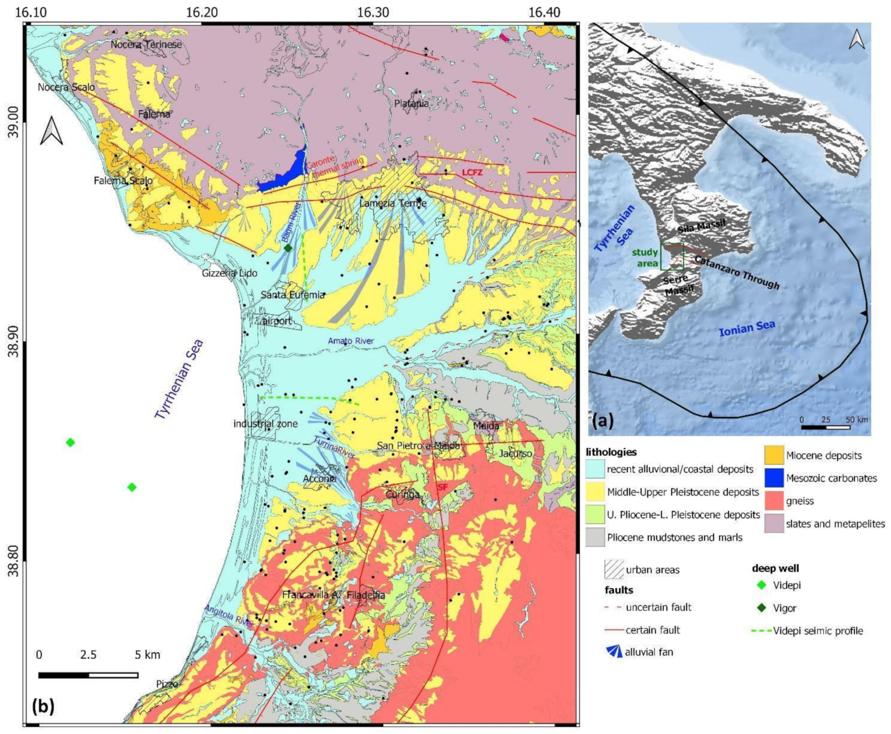
2. Geological Setting

The Sant’Eufemia plain (hereafter SEP) covers an area of ~120 km2 and is located along the Tyrrhenian coast of the Calabria region (southern Italy). The investigated area (Figure 1) is on the westernmost edge of a Neogene-Quaternary sedimentary basin, the so-called “Catanzaro Trough”, placed in the middle sector of the Calabrian Arc (CA). The CA represents a fault-bounded continental fragment within the western Mediterranean orogen, located at the intersection of the E-W-trending Sicilian Maghrebides and NW-SE-trending southern Apennines on the south and the north, respectively. The CA origin is linked to the episodic Neogene roll-back of an NW-dipping subduction zone with the associated opening of backarc basins in the western Mediterranean [27,28]. During Neogene-Quaternary, the backarc extension has produced the progressive eastward migration of the CA, accommodated by NW- and WNW-trending strike-slip faults systems, which are responsible for the Calabrian Arc dissection into structural highs and longitudinal and transversal sedimentary basins [29,30,31], as the Catanzaro Trough. The latter is confined between the Soverato-Lamezia (southward) and Catanzaro-Amantea (northward) strike-slip NW–SE trending fault zones [30]. During the late Miocene, the NW–SE trending fault systems had mainly left lateral kinematics, which switched to right-lateral ones during the Piacenzian-Lower Pleistocene [32].
The CA terranes crop out along the northern and southern sides of the SEP. Along the north side, slates and metapelites (Bagni unit), and orthogneiss (Castagna unit) outcrop; a tectonic window of the Apennines chain made by Mesozoic carbonates complex is also present [31,33]. Along the southern side, Hercynian migmatitic paragneisses of the Serre Massif crop out [34]. On the crystalline basement, the basin-fill succession starts with Upper Miocene terrigenous and evaporitic deposits, outcropping along the Catanzaro Through eastern edge [35,36,37,38,39] and buried in correspondence with the SEP as testified by two deep offshore wells [40]. The basin-fill stratigraphy passes upward to ~350 m thick Pliocene mudstones and marls (time correlative with the Trubi Formation), paraconformably overlain by a ~200 m thick Upper Pliocene—Lower Pleistocene succession composed of weakly cemented sandstones and mudstones [41]. The Middle–Upper Pleistocene deposits, resting directly on Lower Pleistocene deposits and the crystalline basement, consist of continental/shallow marine sands and conglomerates [32,41]. The northern SEP margin is characterised by outcrops of Late Quaternary 60 m-thick alluvial fans (conglomerate and sand) deposits [32].
The northern SEP margin is bounded by the WNW–ESE to WSW–ENE trending Lamezia-Catanzaro Fault System, some segments of which have recently been reactivated as normal faults, testifying by morphotectonic data [42] and they are still active [43]. Along this tectonic lineament, a thermal spring, characterised by Ca-SO4 waters with temperatures up to 38 °C, is close to the Caronte locality [44,45,46,47,48,49]. Southward, the SEP is bounded by a minor north-dipping fault, the Maida Fault, which juxtaposes crystalline rocks with Pliocene–Middle Pleistocene deposits. Westwards, the Maida Fault is displaced by the active N–S-oriented Serre Fault [42].

3. Methods

The methodological approach applied in this work consisted of collecting all the available data related to the main geological, hydrogeological, thermophysical, climate and economic characteristics of the investigated area. Then, the retrieved data were used to produce thematic maps, essential for the correct evaluation and mapping of the geothermal potential of the territory. These thematic maps were constructed considering the climatic conditions (air temperature) and the underground’s stratigraphic, hydrogeological and thermophysical properties (thermal conductivity, volumetric heat capacity, specific heat extraction). Moreover, the costs and potential socio-economic benefits were also considered.
All the evaluations were performed considering an average depth of the BHE of 100 m from the ground level. All the maps are georeferenced in the geographic WGS 84 coordinates system. They have been obtained through geostatistical interpolation (Ordinary Kriging method) in the GIS environment (ESRI—ArcGIS) using suitable semi-variogram models to describe the spatial dependence of the considered parameters [50]. The prediction standard error map for each investigated parameter is reported in the Supplementary Materials (estimated thermal parameters, punctual geothermal potential, etc.).

3.1. Subsoil Stratigraphy

Subsoil data were retrieved from the following: (i) archive of subsurface investigations made accessible by the Italian Institute for Environmental Protection and Research [51], and (ii) boreholes drilling for the Progetto Speciale 26 [52]. Each drilling point, associated with a geographic coordinate, was reported in a geodatabase, including stratigraphic and water table information, in the QGIS software (boreholes location and information in Figure S1 and Table S2, respectively).
This dataset of 208 boreholes was coupled with field observations, deep stratigraphic data (2 offshore exploration wells and two onshore seismic profiles of the “ViDEPI—Visibility of Petroleum Exploration data in Italy” [40] and a 915 m deep borehole of the Vigor project [53]) and geological and geomorphological maps [32,42,54] to reconstruct the geological and stratigraphic relationships between the different lithological units.
Considering that the first 100 m of the subsoil is usually interested in thermal exchanges using vertical closed-loop BHEs [9,15,24,55,56], each borehole was virtually extended, considering homogenous lithostratigraphic features or shortened up to this depth. This depth was also selected to elaborate the geothermal thematic maps.
The lithological information of each borehole was inserted into the database. The lithological units were classified following the modified “Unified Soil Classification System” [57], also used for the Italian Seismic Microzonation studies [58], and according to work [24]. This classification, which distinguishes 16 types of soil [58], is based on the dominant lithology and the hydraulic conditions and was simplified by subdividing soil units into gravel, sand and silt/clay in dry or wet conditions. The geological bedrock was discriminated based on lithology.

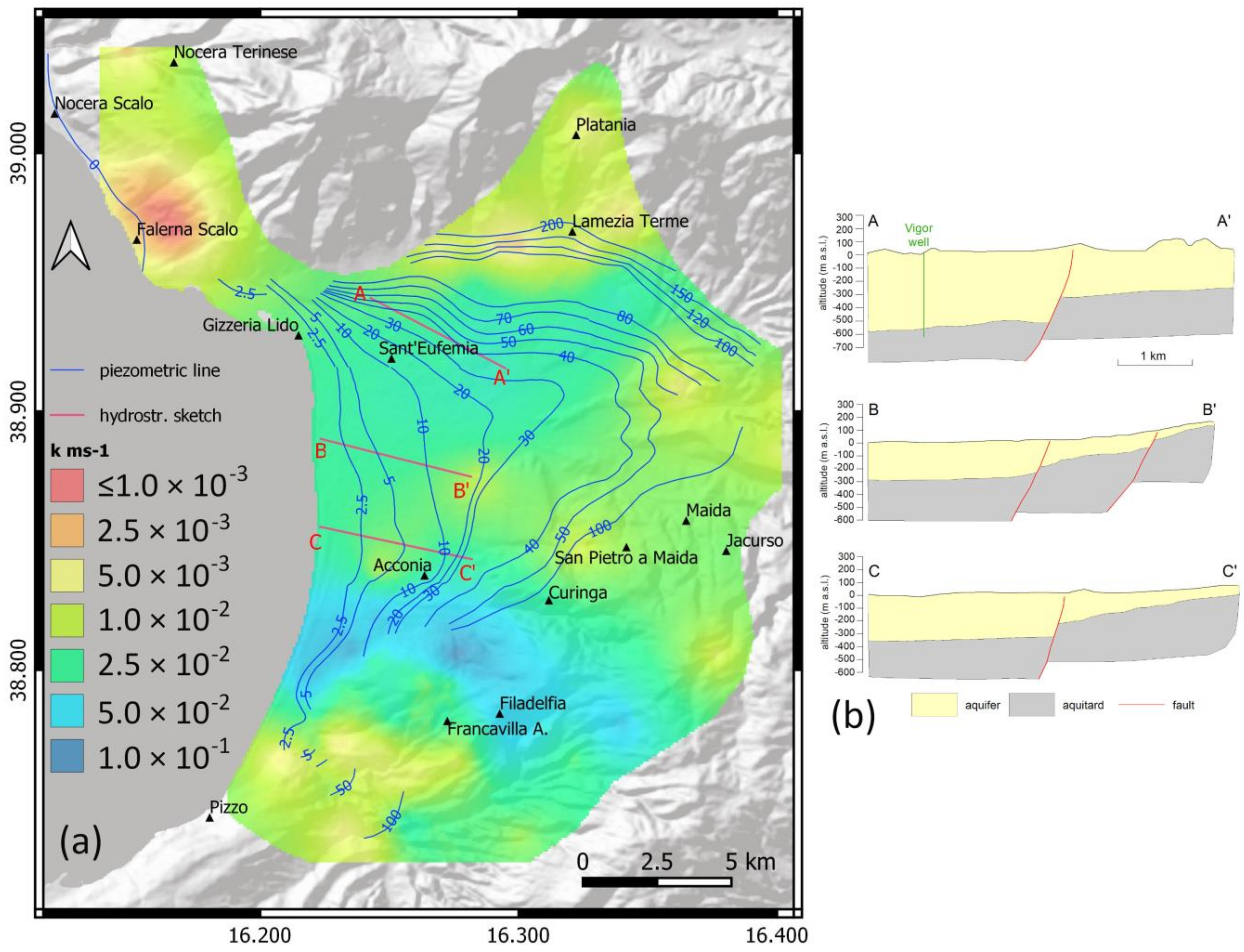
3.2. Hydrostratigraphy

The hydrogeological conditions of the alluvial aquifers must be considered when the heat-exchange potential of the underground is evaluated [9,15,55,56]. This work reconstructed the piezometric surface using the ISPRA [51] and CASMEZ [52] datasets.
The subsoil stratigraphic data were used to reconstruct the hydrostratigraphic framework of the SEP. In detail, the lithological information (mainly in terms of grain size) were converted into hydrogeological units, seen as geologically homogeneous unit (but not necessarily isotropic) with distinctive hydrodynamic properties [22,59]. Furthermore, hydraulic conductivity values were obtained using the static and dynamic piezometric levels data available for the 128 ISPRA boreholes. Finally, following the empirical method proposed by [60], the following equations were used:
T = 2.43 × Q × b Δ h × 2 b Δ h
T = k × b
where T is the transmissivity (m2·s−1); Q is the well discharge (m3·s−1); Δh is the drawdown (m) and b is the saturated aquifer thickness drilled by each well (m).

3.3. Thermophysical Properties of the Lithological Units

The main thermophysical properties of the subsoil, intended as the thermal conductivity (λ, expressed in Wm−1 K−1), volumetric heat capacity (SVC, expressed in MJ m−3 K−1) and the specific heat extraction (SHE, expressed in Wm−1), were retrieved from [61], which reported specific values for the Calabria region lithotypes, [15,62,63,64], and are summarised in Table S1. Concerning the detailed SHE values of each lithotype, these were assigned according to the relationship (3) found by [15] between the SHE rates of the [64], the λ of the different lithology and the operating hours in the heating (Heq) and cooling season (Ceq) as follows:
SHE H , C   = 3.34 ×   λ 2 + 4.54 ×   λ   + 21.63 × 1 + 2400   H eq   or   C eq   × 0.2 / 2400 1800
The SHEH and SHEC (in W m−1) values are related to a total amount of 1244 (Heq) and 772 (Ceq) operating hours, respectively. Therefore, the following simplified function (4) proposed by Commission Delegated Regulation (Eu) 2022/759 (14 December 2021) was used to define the Heq and Ceq in residential spaces as a function of the degree days (cooling degree days: CDD, and heating degree days: HDD):
H eq   or   C eq = 96 + 0.85 ×   CDD   or   HDD
The HDD (1350) and CDD (795) values of the SEP, calculated based on the air temperature, were estimated using the online software degree days (https://www.degreedays.net/ (accessed on 15 January 2023)) assessing a base temperature of 19 °C (i.e., a conventionally fixed temperature for an indoor environment). The data obtained are consistent with those reported in the Presidential Decree n. 412 of 26 August 1993 defined the annual periods the heating systems can operate for private home conditioning (see also D.M. n.383 del 6 October 2022).
All these data, divided by lithology and hydrogeological properties (i.e., saturated or unsaturated), are summarised in Table S2.
These values were also used to define the depth to be drilled to supply a fixed energy requirement for domestic heating and cooling. To define the unitary consumption demand (U) of a standard house (100 m2), the following equation proposed by [10] was used (5):
U (kWh m−2 y−1) = CDD or HDD × 0.0411 + 4.677
Once the consumption U was calculated, it was multiplied by the area of a standard house and divided by the average operating hours (1244 (Heq) and 772 (Ceq)) of the installation during the year. In this way, the power demand in kW can be obtained as follows (6):
PBHE (kW) = U (kWh m−2 y−1) × 100 (m2)/(operating hours)

3.4. Climate Data

Climate data have been taken from the Calabria region’s Arpacal-CFM (Multi-hazard Functional Center). The meteorological stations of Lamezia Terme—Palazzo (24 m a.s.l.), Tiriolo (690 m a.s.l.), Nicastro (400 m a.s.l.) and Cortale (516 m a.s.l.) located in, or nearby, the area under investigation, were used to determine the mean monthly air temperature (reference period 2000–2022) and define the relationship between elevation and local mean atmospheric temperature. As the local climate conditions and altitudes affect the undisturbed soil temperature (T0) [65], the mean annual air temperatures were used to estimate it at each investigated point. In the absence of significant local geothermal anomalies, as in the present study area where the average surface heat flow is in the range of 30–50 mW m−2 [66], the annual average temperature of the first 100 m of the underground can be assumed as the annual mean air temperature [15]. Thus, following the approach of [65], an empirical formula (7), specifically for the investigated territory, was developed as follows:
T0 = 0.7626 × [(−0.0052 × Z +18.163) + 3.6403]
where Z is the elevation (m a.s.l.) of each borehole, obtained from the digital terrain model (DTM) 20 × 20 m (Geoportale Nazionale, n.d.).

3.5. Geothermal Potential Estimation

To estimate the geothermal potential, the following G.POT method developed by [9] was applied:
Q BHE = a × T 0   T lim × λ × L × t c 0.619 t c × loglog   u s + 0.532 t c 0.962 × loglog   u c 0.455 t c   1.619 + 4 π λ ×   R b  
With a = 8 or 7.01 × 10⁻² if QBHE is expressed in W or MWh y−1, respectively. (T0-Tlim) represents the maximum possible thermal alteration of the fluid, λ is the thermal conductivity of the ground, “L” is the borehole length and Rb is the thermal resistance of the borehole. t’c = tc/ty (ty = 365 days), u’s = r2b/4αts (rb = borehole radius) and u’c = r2b/4αtc represent three nondimensional parameters depending on the simulation time (ts = 50 years) and length of the load cycle (tc = 120 days).
This empirical method permits the definition of the mean thermal load that can be extracted or injected in the subsoil, characterised by specific conditions during the year, avoiding major variations of the heat transfer fluid during the operational life of the geothermal system. This method, which is essentially based on the temperature difference between the ground and the heat carrier fluid, has been widely used in several studies [24,26,55,56,67,68] and relies on different variables. These latter are linked to the thermal properties of the ground (i.e., λ, SVC and undisturbed ground temperature) and of the borehole (depth, radius, thermal resistance), and the operational and design parameters of the low-temperature geothermal plant (minimum or maximum temperature reached by the fluid, clime, operational life). However, most of the works that applied the G.POT method used it only to estimate the geothermal potential for the heating mode. In our case, considering the climatic conditions of the study area, the G.POT method was applied in dual mode, considering both the heating winter and the cooling summer season. The operation in cooling mode during summer can also help, at least partially, compensate for the heat extraction during winter, reducing the ground’s thermal drift [67]. For this purpose, the threshold fluid temperature, one of the essential parameters of the [9] method, has been assessed for both operating modes. The parameters used to apply the G.POT algorithm are summarised in Table 1.

3.6. Economic Cost Estimation

Compared to conventional and renewable thermal technologies, the cost of the BHE installation is usually higher due to the costs associated with drilling the vertical boreholes.
For this reason, the focus was estimating the drilling costs considering the power demand of 5 kW (values calculated by Equations (5) and (6)). The cost analysis was based on the price list of public building works of the Calabria region (https://www.regione.calabria.it/.../prezziariooopp/ (accessed on 15 January 2023)). In detail, non-coring drilling and its different costs depending on the drilled terranes (sedimentary infill or crystalline bedrock) and depth (greater or lesser than 30 m) (Table 2) were considered. Furthermore, the costs of the provisional coatings needed to exclude hole stability problems during the drilling were considered. The drilling in the sedimentary infill and crystalline bedrock was considered the provisional coatings for the entire hole length and only for the segment under the water table, respectively.

4. Results and Discussion

4.1. Climate Parameters and Classification

Mean annual temperatures for the investigated area range between 14.8 and 18.3 °C, with minimum and maximum average monthly values of 7 and 25.7 °C, respectively, outlining similar climate conditions for the study area. Based on the air temperature, the climate classifications of all the Italian municipalities are specified by the Presidential Decree n. 412 of 26 August 1993. Six classes, from A to F, from the warmest to the coolest (https://luceegasitalia.it/ (accessed on 15 January 2023)), are established, each defining the annual periods that the heating systems can work for private home conditioning. This classification is based on the (heating) degree day (DD) that corresponds to a daily positive difference between 19 °C (i.e., a conventionally fixed temperature for an indoor environment) and the outdoor average daily temperature. According to this classification, the municipalities in the investigated area of the SEP show an HDD (heating degree days) value of 1350, which corresponds to Climate Zone C, which defines a heating season of 122 days between the 22 of November and the 23 of March (Presidential Decree. DPR 26 August 1993, n. 412 and D.M. n.383 del 6 October 2022). However, the same Italian normative does not define the CDD (cooling degree days), which were thus estimated using the online software degree days (https://www.degreedays.net/ (accessed on 15 January 2023)). Additionally, a base temperature of 19 °C, returning a value of 795 and a cooling season of 120 days. The heating or cooling period (in days) depends on the different climatic zones and the area to be studied. Representative European building types are compared using H&C load analysis by [69].

4.2. Hydrostratigraphic Reconstruction

The SEP hydrograph pattern consists of the following four main drainage systems: (i) the Bagni River, located in correspondence with the SEP northern margin with an NS and WE (toward the mouth) drainage direction, characterised by torrential watercourse; (ii) the Amato River, in the middle SEP sector, is the main drainage system of the area with a catchment of ~440 km2; (iii) the Turrina River with a torrential watercourse and a mainly SE-NW drainage direction; (iv) the Angitola River, with the mouth in the southernmost sector of the SEP, is characterised by a mainly SE-NW drainage direction and a catchment of ~190 km2.
The groundwater flow direction, inferred by the piezometric map (reconstructed based on [51,52] datasets) (Figure 2), shows a substantial similarity with the hydrography. Indeed, an N-S-oriented prevalent groundwater flow direction can be observed in the northern sector. On the other hand, W-E and SW-NE groundwater flow directions characterise the middle and southern SEP sectors, respectively.
According to stratigraphic and geological data derived from the literature investigation surveys (wells, deep boreholes and seismic profiles), bibliographic sources and field observations, two main hydrostratigraphic units in the SEP were identified. The shallowest one, representing a phreatic aquifer, includes the sedimentary succession from Upper Pliocene to Holocene. A complex hydrostratigraphic architecture characterises this unit due to vertical and lateral variations in lithological units. Still, it is considered a unique hydrostratigraphic unit at the scale of the whole SEP.
The second hydrostratigraphic unit consists of the Pliocene mudstones and marls (~350 m thick), which act as aquitard at the bottom of the phreatic aquifer.
The simplified hydrostratigraphic framework of the SEP is characterised by a general thickening of the aquifer toward the west due to the normal faults (southwest and west/northwest dipping along the northern and southern SEP sectors, respectively), which lower the aquitard (Pliocene mudstones and marls). Locally, the aquifer has a thickness of the order of 600 m as testified in the SEP northern sector by the deep borehole Vigor [53], which drilled the top of the Pliocene mudstones and marls at 600 m of depth.
While a porous aquifer in sedimentary rocks characterises the plain, fractured aquifers are present along the SEP northern and southern margins, where low-grade (slates and metapelites) and high-grade (gneiss) metamorphic rocks crop out, respectively.
The lowest hydraulic conductivity (k) values (≤10−3 m/s) are calculated in the Falerna Scalo area (outside the SEP aquifer system), where the Miocene succession lies on the crystalline bedrock. Around Lamezia Terme, the k value increase from 5 × 10⁻³ m/s, at the contact between crystalline bedrock and alluvial fans, to 2.5 × 10⁻² m/s southward, where the alluvial deposits are thicker. In the Amato River alluvial plain the k has values of 2.5 × 10⁻² m/s. Along the middle eastern margin of the SEP, where the aquifer is mainly made by Upper Pliocene-Lower Pleistocene (including sandstones and mudstones), the calculated k values are of the order of 5 × 10⁻³ m/s. The highest k values (5 × 10⁻³ < k < 10−2 m/s) are calculated in the area between Curinga and Filadelfia, where the wells are mainly drilled in the crystalline fractured and weathered bedrock. Southward, in the Angitola catchment k has values of 5 × 10⁻³–5 × 10⁻² m/s, reflecting the more significant number of fine-grained sediments in the aquifer testified by the outcropping lithological unit and the well-logs.

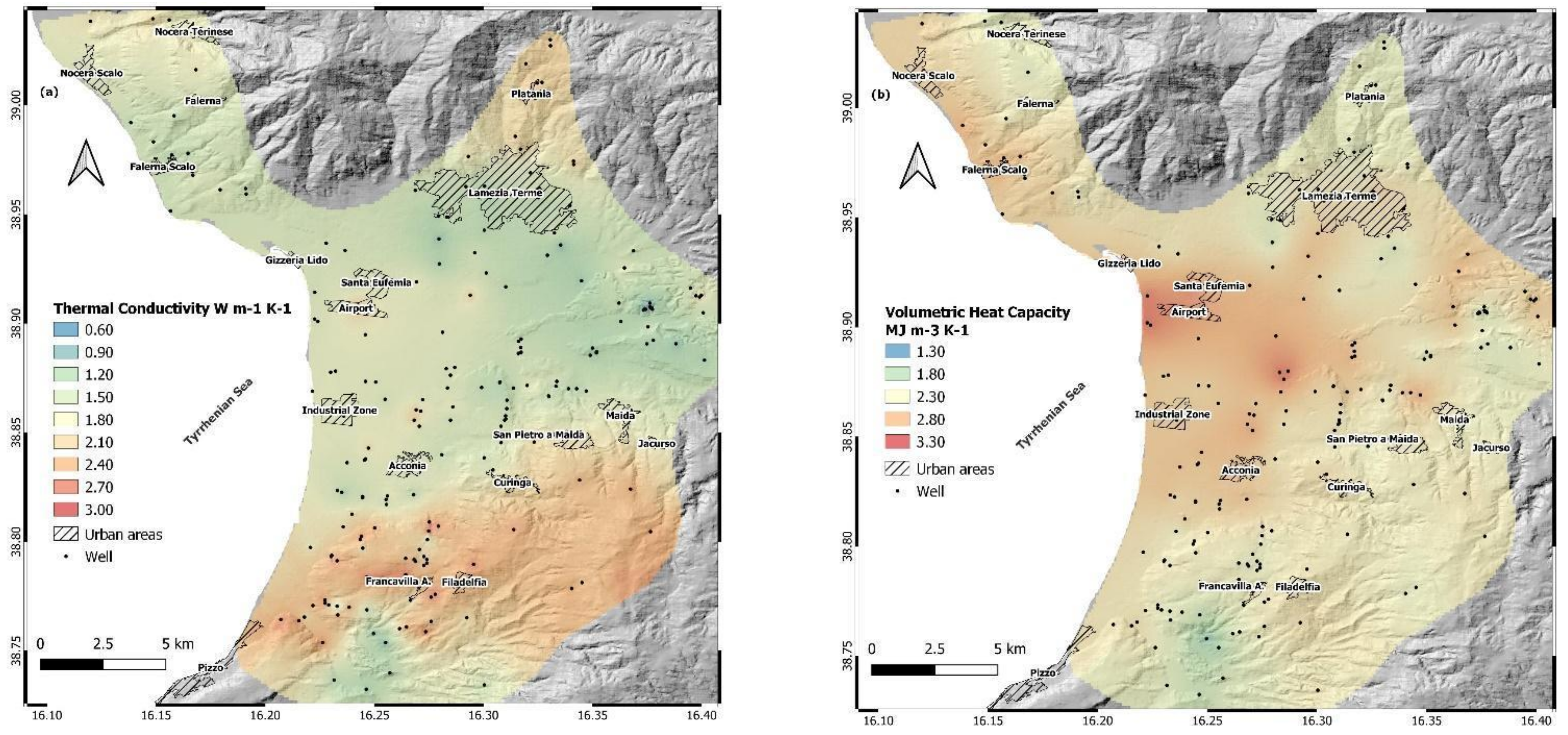
4.3. Thermophysical Properties of the Underground

The thermal conductivity (λ) and the volumetric heat capacity (ρc) have been defined for each stratigraphic unit using the lithostratigraphic information of the geognostic drillings and the hydrogeological saturation level (Table S2). The results are reported in the maps of Figure 3a,b. The values of λ in the SEP range between 0.69 and 2.90 W m−1 K−1, with a mean value of 1.74 W m−1 K−1. The heterogeneity in terms of granulometric characters of the sedimentary deposits, the depth of bedrock and saturation level and the saturated thickness allowed us to define the following three main areas: (i) high, (ii) medium and (iii) low thermal conductivity areas. The north and south boundaries of the study area have shown the highest conductivity values (between 1.9 and 2.75 W m−1 K−1) as they are characterised by the thin thickness of the sedimentary infill, which thus poorly influenced the weighted λ along the first 100 m of the subsoil. The crystalline basement, made up of slates and metapelites to the north and gneiss to the south, is found in outcrops and/or a few meters from the surface. Some of the most important urban areas of the SEP are located in these sectors, such as Lamezia Terme (the northern border), Curinga and Filadelfia (Figure 3a).
The central portion of the study area is characterised by a gradual decrease in the λ values moving from the coast, where the industrial zone, the international airport and Sant’Eufemia town are located, to the east side (values < 1 W m−1 K−1) (Figure 3a). This represents the portion with the highest thicknesses (up to 600 m) of the lithologically-homogeneous sedimentary infill. In this area, the westward thickening of the saturated portion (Figure 2a) of the 100 m considered (Table S2) contributes to an increase in the conductivity values (up to 2 W m−1 K−1).
The volumetric heat capacity is moderately homogeneous throughout the investigated area (Figure 3b). In fact, in most of the SEP, SVC values range between 1.8 and 2.3 MJ m−3 K−1.
The coastal side, where the international airport and the industrial zone are located, differs from this range. Near the coastal area, the elevated presence of permeated deposits (sands to clays) gives rise to SVC values generally higher than 3 MJ m−3 K−1, with a maximum of 3.33 MJ m−3 K−1.
The lowest SVC values (i.e., <1.7 MJ m−3 K−1) are found in the correspondence of a small portion of the southern sector (Angitola catchment) where the deepest saturation levels (>50 m from the ground) and the increased thickness of the sedimentary fill favour the decrease in SVC values (Figure 3b).

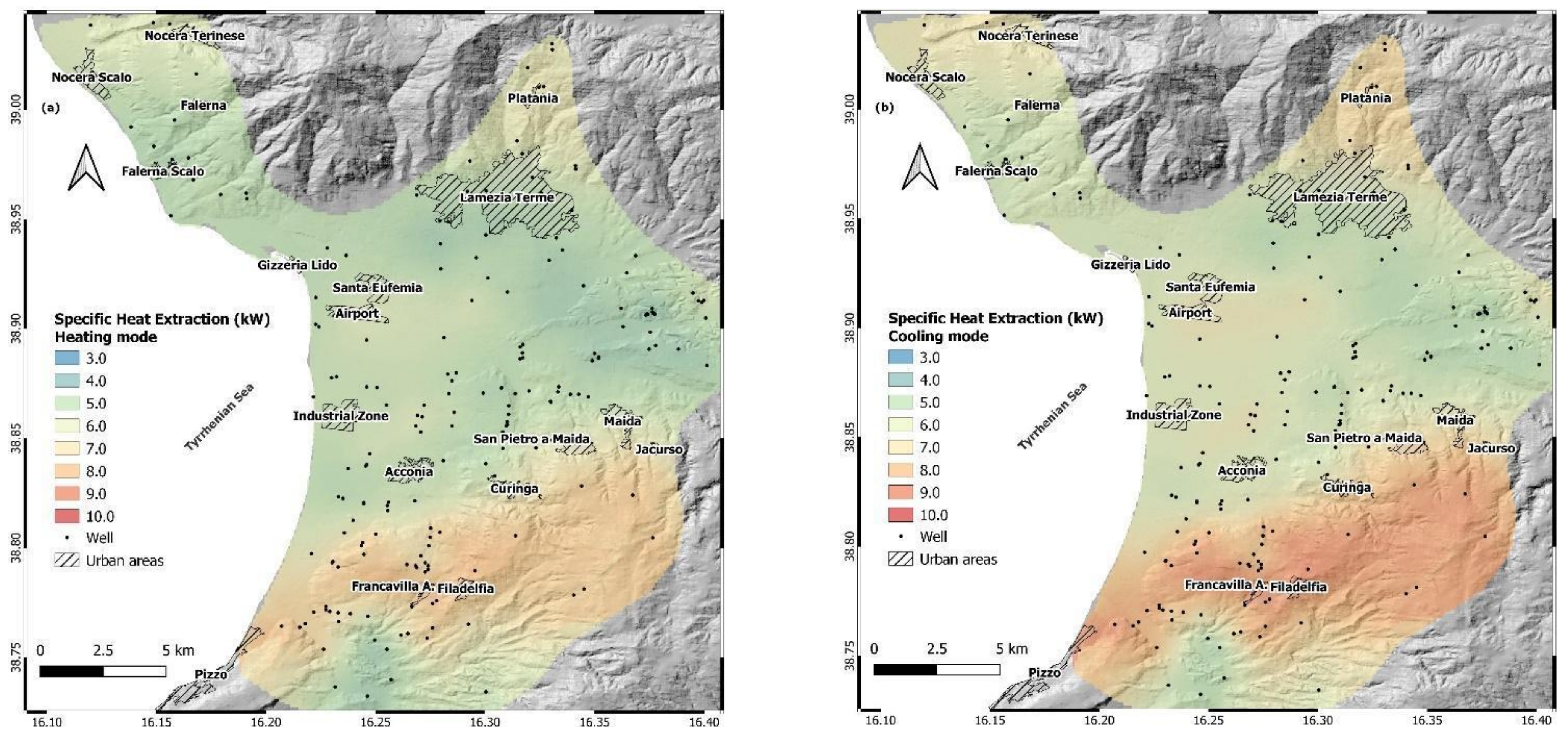
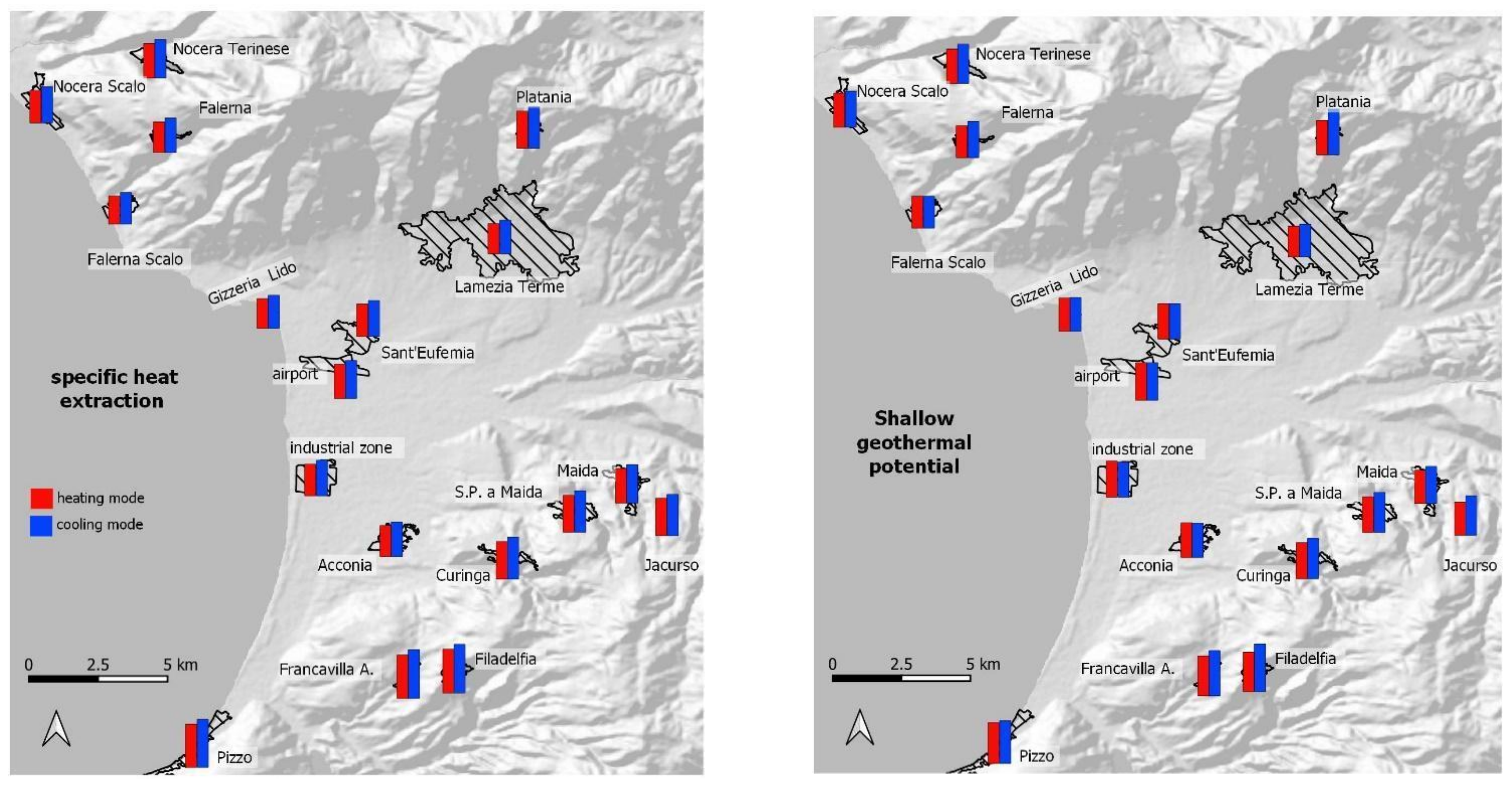
4.4. Specific Heat Extraction

In this work, Equation (3) proposed by [15] was used to define both the specific heat extraction (sHE, in kW) related to the heating (Heq) and cooling seasons (Ceq). The values for each well are reported in Table S2. As expected, in the study area, the specific heat extraction rate (Figure 4a,b) increases with increasing thermal conductivity (Figure 3a). In addition, by comparing the map for the heating mode and the cooling mode (Figure 4a,b), this value increases with decreasing in the operating hours (1244 (Heq) and 772 (Ceq)).
The minimum and maximum values calculated on the verticals of investigation are 3.05 kW–8.71 kW (mean: 5.83 kW) and 3.40 kW–9.7 kW (mean: 6.49 kW) for heating and cooling modes, respectively. The central portion of the plain shows the lowest sHE values (between 4.4 kW and 6 kW), which tend to decrease moving inland (Figure 4a,b). This effect is probably related, as previously discussed for the thermal conductivity, to a gradual lowering of the piezometric level (Figure 2), given the overall homogeneity from a lithological point of view.
The higher values of sHE are recorded in the southern and northern portions of the studied area agreeing with the maximum λ values and the presence of crystalline basement outcrops (sHE values between 57 and 78 W m−1). The heating and cooling modes maps show an equal distribution of values with higher average sHE for the cooling mode given the lower operating hours.

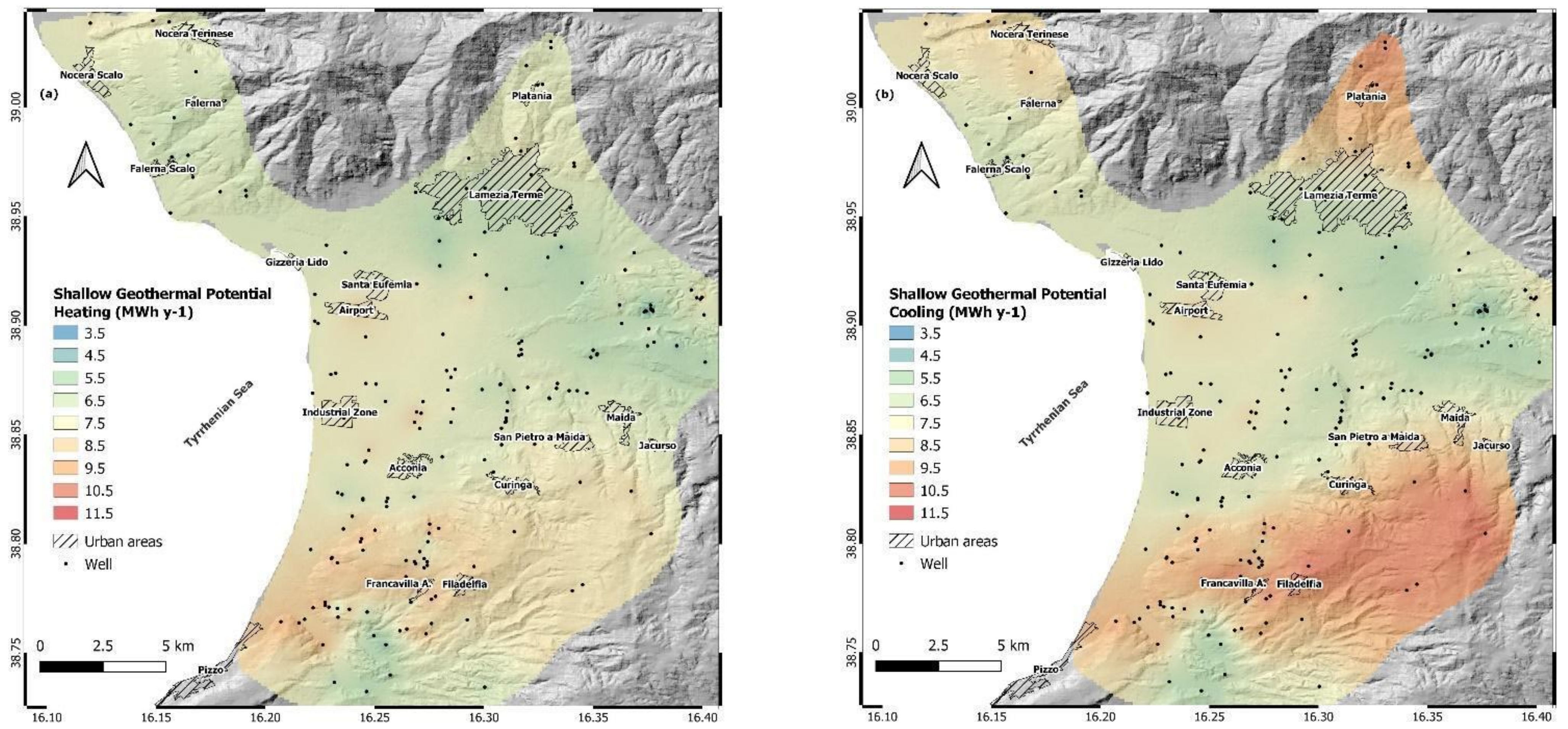
4.5. Geothermal Potential for Heating and Cooling Mode

The maximum amount of shallow geothermal energy to be annually extracted by a BHE system with a specific length (100 m) to provide space heating (Figure 5a) and cooling (Figure 5b) energy demand for the residential sector in SEP, is estimated according to the G.POT method described in Section 3.5. Input data for the thermal energy transfers are summarised in Table 1. Figure 5a,b show that a geothermal energy supply between 3.61 and 10.56 MWh can be extracted annually for heating purposes from the underground depending on the location, with a mean value of 7.24 MWh y−1. Whereas a range of 3.72–11.47 MWh y−1, with a mean of 7.59 MWh y−1 is the thermal energy that can be sustainably ceded for cooling purposes. The geothermal potential map defines that the highest capacity to extract and release heat from and to the ground is found in the southern portion of the territory, between the municipalities of Pizzo and Curinga. In this area, values generally higher than 7 MWh y−1, for both cooling and heating purposes, with peaks of ~10.5 MWh y−1 (cooling), are observed where the crystalline basement, with relatively high thermal conductivity, is present (Figure 1).
Moving northward, the increase in the thicknesses of the sedimentary infill (with variable piezometric level—Figure 2a) drastically drops down the geothermal potential, resulting in values generally <6.0 MWh y−1. The remaining part of the SEP is characterised by values between ~4.70 and ~7.0 MWh y−1, with the lowest potentials located in the proximity of the Angitola catchment (southern portion of the plain to the east of Pizzo municipality) and between the urban centres of Maida and Lamezia Terme where the high thicknesses of the sedimentary infill and the thick unsaturated zone above the shallow aquifer control the low potential for both heating and cooling (Figure 5a,b). Overall, the geothermal potential is mainly controlled by the thermal conductivity of the lithotypes and the hydrogeological conditions, considering the ground temperature as relatively homogeneous throughout the whole area (12.5–16.6 °C), as well as the values of SVC (Figure 3b). Therefore, the geothermal potential for heating purposes estimated for the SEP can be regarded as a medium-high potential, being generally >7.2 MWh y−1, when compared to other areas where G.POT has applied [24,26,55,56,67,68]. With respect to the cooling potential, few works focused on this issue; thus, a reliable comparison is difficult. Recently, [55,56] estimated the geothermal potential (for both heating and cooling modes) for the Murcia Region (Spain), where similar climatic conditions to those of this work occur. These authors reported that for space cooling, the potential of the Murcia Region varies from 1.8 to 14.2 MWh y−1, with 6.7 as the mean value, outlining similar conditions to those estimated for the SEP area.

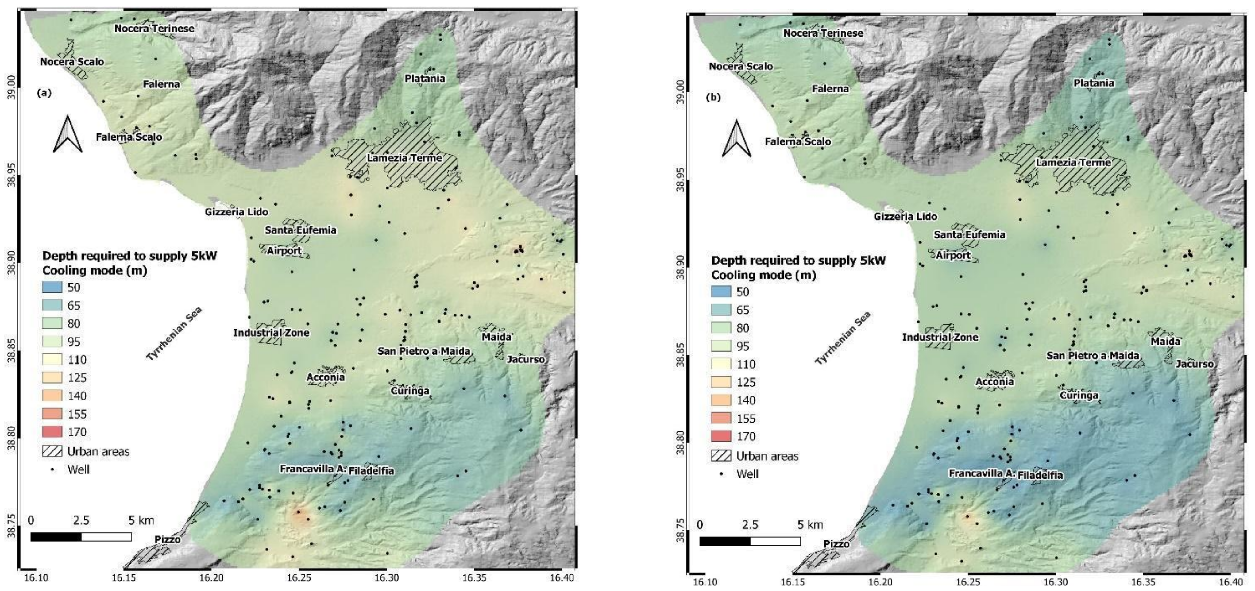
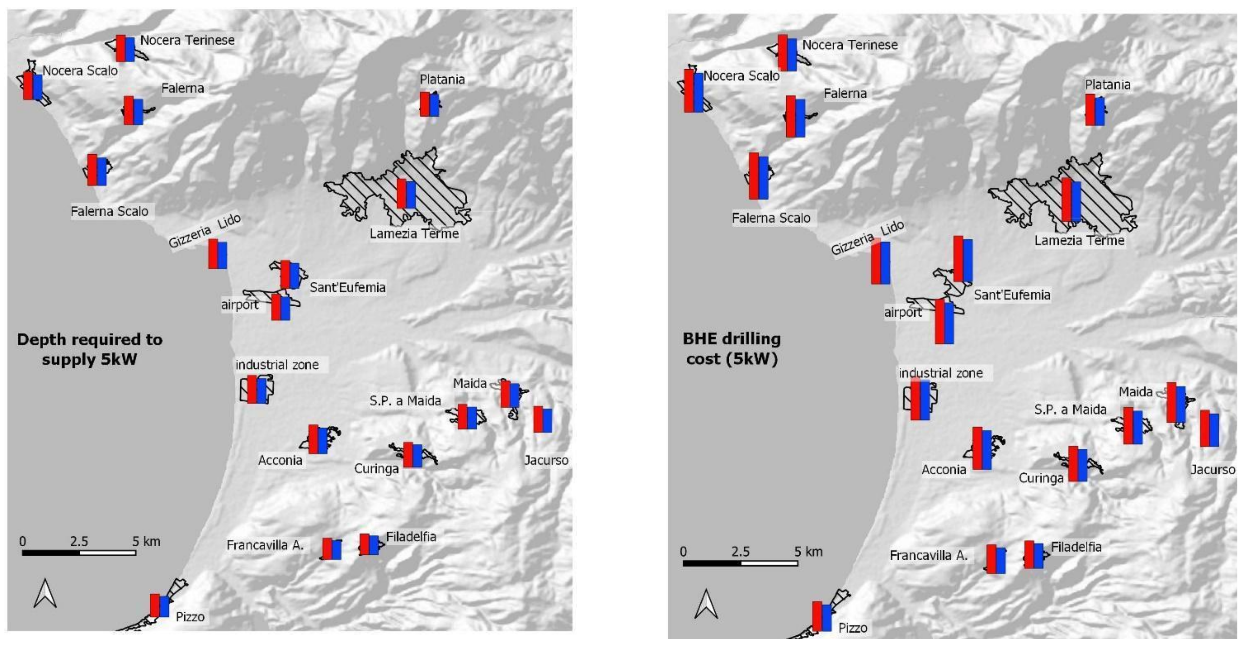
4.6. Depth to Be Drilled for Vertical Closed-Loop BHE Systems

Following Equations (3) and (4), a mean consumption of 60 kWh m−2 y−1 and 38 kWh m−2 y−1 for domestic heating and cooling, respectively, and a power demand of ~5.0 kW for a standard domestic environment, were defined.
Considering this, the depth to be drilled to supply 5.0 kW was estimated for each investigated point (Figure 6a,b). For heating mode, the drilling depths are in the range of 57–164 m, with an average value of 90 m. Similarly, for cooling mode, the drilling depths are in the range between 51 and 147 m, although with a lower average value of 81 m. A general increase in the depth is required to achieve 5.0 kW, moving from the coast to the inner part of the investigated area (Figure 6a,b), in agreement with the general decrease in the thermal conductivity (Figure 3a) and specific heat extraction rates (Figure 4a,b) of the sedimentary infill.
The most favourable areas (for both heating and cooling) are the southern ones between the urban centres of Pizzo, Filadelfia and Curinga, with values below ~70 m. The northern portions (north of the urban area of Lamezia Terme), where the crystalline basement outcrop, are also characterised by low estimated depth with values less than ~90 m.
Overall, as observed in the previous sections, the maps for the heating and cooling modes show an equal distribution of values but with a general lower depth to be drilled for the cooling mode, given the higher sHE values detected.

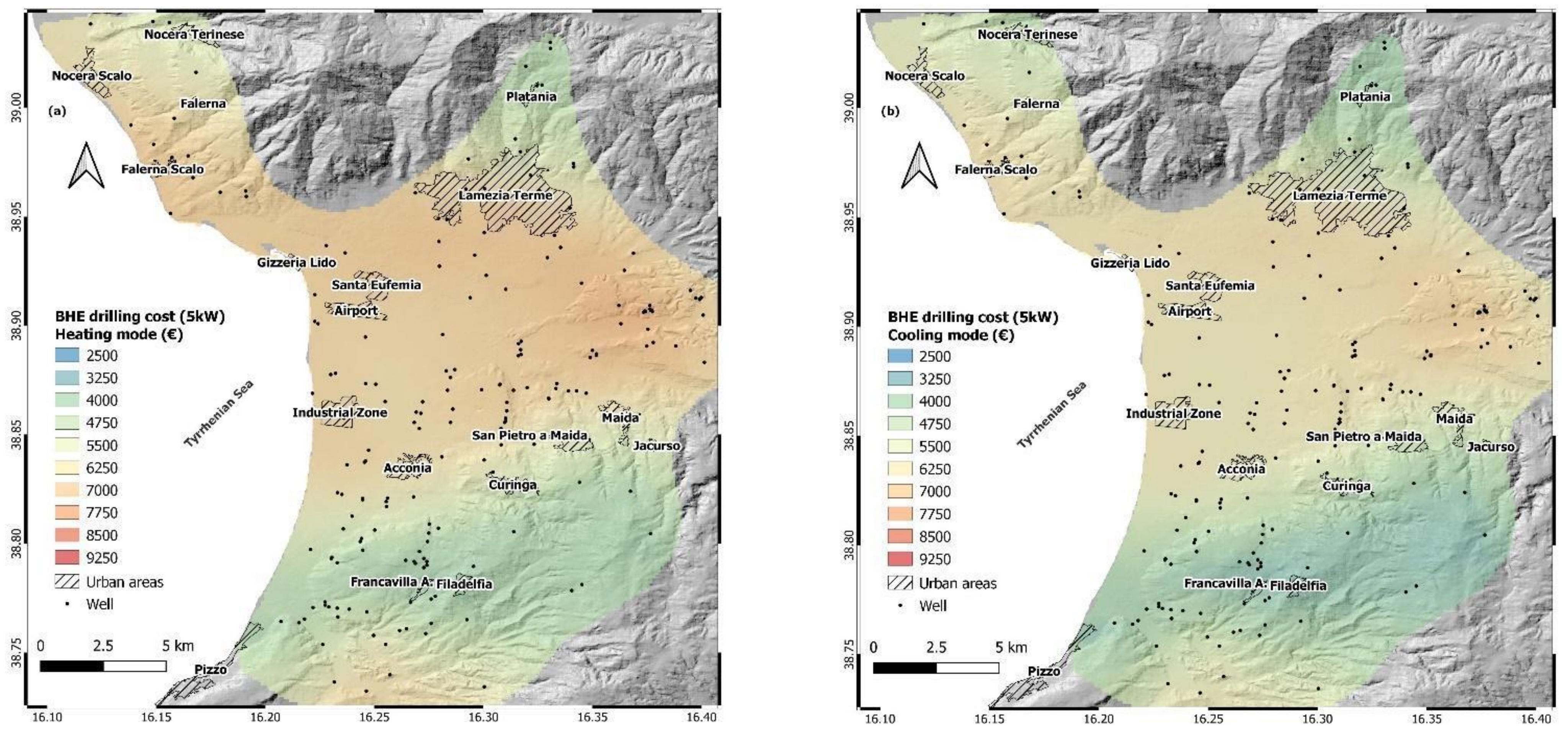
4.7. Economic Analysis

Considering the depth required to supply 5kW for both heating and cooling modes (Figure 6), the costs for non-coring drilling, including those for the provisional coatings, were analysed.
Referring to the heating mode, the minimum drilling cost of EUR ~3200.00 was estimated in the southern sector (Figure 7a), where the depth required to supply 5kW is lower, thanks to the presence of the high thermal conductive crystalline bedrock. The short length of the drilling, in addition to the unnecessary provisional coatings above the water table, allows for maintaining a low cost despite the higher cost of drilling the crystalline rocks (Table 2). Low costs, between EUR ~4500.00 and ~5500.00, can be observed in the northern sector (Figure 5a), where also the outcropping crystalline bedrock (Figure 1) allows for keeping low the depth required to supply 5 kW (Figure 6a). The maximum cost (EUR > 7500.00 €) is instead calculated in the middle eastern sector (Figure 7a) due to the higher depth required to supply 5 kW (Figure 6a) related to the presence of thick sedimentary infill (Figure 1) and deep piezometric level (Figure 2), which added together create a low thermal conductivity.
About the cooling mode, the spatial distribution of the drilling costs (Figure 7b) is the same as the heating mode but with lower average values of EUR 550.00 due to the lower depth required to supply 5kW (Figure 6b). Therefore, the minimum and maximum costs for the cooling mode are EUR ~2800.00 and ~7800.00, respectively. Obviously, given the reversibility of the geothermal probes that can be used in a double-modality (heating and cooling), the costs that should be considered are those related to the deepest drillings. This means that having a greater length available, the mode that requires less length will be likely able to supply even higher thermal energy to the system.
To provide a useful tool for the local decision-makers, the mean values of sHE, QBHE, drilling depth and costs for both heating and cooling modes are calculated for the main municipalities and strategic sites (industrial areas and airport) (Table 3 and Figure 8).
Considering a constant geothermal heat pump and its installation costs, the realisation of the BHE system is cheaper in the Filadelfia and Francavilla towns, with costs ≤ EUR 4300 and 3800 for heating and cooling, respectively. The higher costs are instead recognised for the Falerna Scalo and Gizzeria Lido ≥ EUR 6800 and 6250 to realise a heating and cooling BHE system, respectively, are needed.
When comparing our results and the characteristics of the study area (e.g., sHE, λ) to those reported by [10], a payback time (i.e., the time required for the energy cost to reach the installation one) of 7–8 years seems reasonable. Thus, this could be a feature of paramount importance to accompany these urban centres through an effective green energy transition, consequently lowering GHGs emissions.

5. Conclusions

In this work, a detailed study of the geological, hydrogeological and thermophysical properties of the subsoil of the SEP has been carried out to define the heat-exchange potential for heating and cooling uses.
The following two main zones have been identified based on the geothermal potential, calculated using the G.POT algorithm [9]: (i) the north and south SEP margins, characterised by fractured aquifers in the crystalline bedrock, showing the highest geothermal potential values (generally >7 MWh y−1, with peaks of ~10.5 MWh y−1) for both cooling and heating modes; (ii) the sedimentary aquifers in the central portion of SEP and Angitola catchment with medium (toward the coast) to low (inland) geothermal potential values (between ~4.70 and ~7.0 MWh y−1), depending on the piezometric depth. Overall, the heating and cooling modes show a comparable spatial distribution of all thermophysical parameters. The cooling mode highlights higher absolute values for geothermal potential and specific heat extraction and lower absolute values for depth and drilling costs, both related to the lower requested operating hours.
The different geothermal energy requirements influence the depth to be drilled in the studied area to reach a 5.0 kW domestic energy demand for a 100 m2 house (Figure 6) for both heating (from 57 to 164 m) and cooling (from 51 to 147 m) use. The different depth also drives the final drilling costs, which range from EUR 3200 to 8700 for the heating mode and from EUR 2800 to 7800 for the cooling mode.
Overall, the study made it possible to identify the most suitable areas for the realisation of BHE systems in the Filadelfia and Francavilla towns with costs ≤ EUR 4300 and 3800 for heating and cooling, respectively. On the other hand, the higher costs are instead recognised for the Falerna Scalo and Gizzeria Lido areas, with costs ≥ EUR 6800 and 6250, respectively.
The estimation of the shallow geothermal potential of the Sant’Eufemia plain for the heating and cooling system and its economic evaluation corresponds to the first detailed approach at the local scale applied to the Calabria region. This approach will be extended to the whole region to provide a powerful tool for the energy transition.

Supplementary Materials

The following supporting information can be downloaded at: https://www.mdpi.com/article/10.3390/geosciences13040110/s1, Figure S1: Boreholes location; Figure S2: Prediction standard error of thermal conductivity and volumetric heat capacity; Figure S3: Prediction standard error of specific heat extraction; Figure S4: Prediction standard error of shallow geothermal potential; Figure S5: Prediction standard error of estimated depth for 5 kW; Figure S6: Prediction standard error of drilling; Table S1: Thermal conductivity and volumetric heat capacity values; Table S2: Boreholes information and calculations.

Author Contributions

Conceptualisation, G.V., G.C. and M.T.; methodology, G.V., G.C. and M.T.; software, G.V. and G.C.; validation, M.T., R.D.R., R.D. and C.A.; formal analysis, R.D.R., R.D. and C.A.; investigation, G.V., G.C. and M.T.; resources, R.D.R. and C.A.; data curation, G.V. and G.C.; writing—original draft preparation, G.V., G.C. and M.T.; writing—review and editing, R.D.R., R.D. and C.A.; visualisation, G.V., G.C.; supervision, R.D.R., R.D. and C.A.; project administration, R.D.R.; C.A.; funding acquisition, R.D.R.; C.A. All authors have read and agreed to the published version of the manuscript.

Funding

This research was funded by PNRR 2023-2026, grant number (ECS: 00000009; CUP: H23C22000370006; Calabria region).

Acknowledgments

The project Tech4You has supported the work (ECS: 00000009; CUP: H23C22000370006; Calabria region), in the frame of the PNRR 2023-2026. ESRI—ArcGIS software is licensed by Laboratorio Marino SILA (University of Calabria).

Conflicts of Interest

The authors declare no conflict of interest.

References

  1. Moya, D.; Aldás, C.; Kaparaju, P. Geothermal Energy: Power Plant Technology and Direct Heat Applications. Renew. Sustain. Energy Rev. 2018, 94, 889–901. [Google Scholar] [CrossRef]
  2. Rybach, L.; Mongillo, M. Geothermal Sustainability—A Review with Identified Research Needs. Trans. Geotherm. Resour. Counc. 2006, 30, 1083–1090. [Google Scholar]
  3. Zhu, J.; Hu, K.; Lu, X.; Huang, X.; Liu, K.; Wu, X. A Review of Geothermal Energy Resources, Development, and Applications in China: Current Status and Prospects. Energy 2015, 93, 466–483. [Google Scholar] [CrossRef]
  4. Lund, J.W.; Toth, A.N. Direct Utilization of Geothermal Energy 2020 Worldwide Review. Geothermics 2021, 90, 101915. [Google Scholar] [CrossRef]
  5. Moeck, I.S. Catalog of Geothermal Play Types Based on Geologic Controls. Renew. Sustain. Energy Rev. 2014, 37, 867–882. [Google Scholar] [CrossRef] [Green Version]
  6. Florides, G.; Kalogirou, S. Ground Heat Exchangers-A Review of Systems, Models and Applications. Renew. Energy 2007, 32, 2461–2478. [Google Scholar] [CrossRef]
  7. Chow, T.T.; Long, H.; Mok, H.Y.; Li, K.W. Estimation of Soil Temperature Profile in Hong Kong from Climatic Variables. Energy Build. 2011, 43, 3568–3575. [Google Scholar] [CrossRef]
  8. Omer, A.M. Ground-Source Heat Pumps Systems and Applications. Renew. Sustain. Energy Rev. 2008, 12, 344–371. [Google Scholar] [CrossRef]
  9. Casasso, A.; Sethi, R.G. POT: A Quantitative Method for the Assessment and Mapping of the Shallow Geothermal Potential. Energy 2016, 106, 765–773. [Google Scholar] [CrossRef]
  10. Gemelli, A.; Mancini Adriano, A.; Longhi, S. GIS-Based Energy-Economic Model of Low Temperature Geothermal Resources: A Case Study in the Italian Marche Region. Renew. Energy 2011, 36, 2474–2483. [Google Scholar] [CrossRef]
  11. García-Gil, A.; Epting, J.; Garrido, E.; Vázquez-Suñé, E.; Lázaro, J.M.; Sánchez Navarro, J.Á.; Huggenberger, P.; Calvo, M.Á.M. A City Scale Study on the Effects of Intensive Groundwater Heat Pump Systems on Heavy Metal Contents in Groundwater. Sci. Total Environ. 2016, 572, 1047–1058. [Google Scholar] [CrossRef] [PubMed]
  12. Ondreka, J.; Rüsgen, M.I.; Stober, I.; Czurda, K. GIS-Supported Mapping of Shallow Geothermal Potential of Representative Areas in South-Western Germany—Possibilities and Limitations. Renew. Energy 2007, 32, 2186–2200. [Google Scholar] [CrossRef]
  13. Schiel, K.; Baume, O.; Caruso, G.; Leopold, U. GIS-Based Modelling of Shallow Geothermal Energy Potential for CO2 Emission Mitigation in Urban Areas. Renew. Energy 2016, 86, 1023–1036. [Google Scholar] [CrossRef]
  14. Noorollahi, Y.; Arjenaki, H.G.; Ghasempour, R. Thermo-Economic Modeling and GIS-Based Spatial Data Analysis of Ground Source Heat Pump Systems for Regional Shallow Geothermal Mapping. Renew. Sustain. Energy Rev. 2017, 72, 648–660. [Google Scholar] [CrossRef]
  15. Viesi, D.; Galgaro, A.; Visintainer, P.; Crema, L. GIS-Supported Evaluation and Mapping of the Geo-Exchange Potential for Vertical Closed-Loop Systems in an Alpine Valley, the Case Study of Adige Valley (Italy). Geothermics 2018, 71, 70–87. [Google Scholar] [CrossRef]
  16. Cannata, C.B.; Cianflone, G.; Vespasiano, G.; De Rosa, R. Preliminary Analysis of Sediments Pollution of the Coastal Sector between Crotone and Strongoli (Calabria—Southern Italy). Rend. Online Soc. Geol. Ital. 2016, 38, 17–20. [Google Scholar] [CrossRef]
  17. Cianflone, G.; Vespasiano, G.; Tolomei, C.; De Rosa, R.; Dominici, R.; Apollaro, C.; Walraevens, K.; Polemio, M. Different Ground Subsidence Contributions Revealed by Integrated Discussion of Sentinel-1 Datasets, Well Discharge, Stratigraphical and Geomorphological Data: The Case of the Gioia Tauro Coastal Plain (Southern Italy). Sustainability 2022, 14, 2926. [Google Scholar] [CrossRef]
  18. Vespasiano, G.; Cianflone, G.; Romanazzi, A.; Apollaro, C.; Dominici, R.; Polemio, M.; De Rosa, R. A Multidisciplinary Approach for Sustainable Management of a Complex Coastal Plain: The Case of Sibari Plain (Southern Italy). Mar. Pet. Geol. 2019, 109, 740–759. [Google Scholar] [CrossRef]
  19. Vespasiano, G.; Cianflone, G.; Cannata, C.B.; Apollaro, C.; Dominici, R.; Rosa, R.D. Analysis of Groundwater Pollution in the Sant’Eufemia Plain (Calabria—South Italy). Ital. J. Eng. Geol. Environ. 2016, 16, 5–15. [Google Scholar] [CrossRef]
  20. Vespasiano, G.; Notaro, P.; Cianflone, G. Water-Mortar Interaction in a Tunnel Located in Southern Calabria (Southern Italy). Environ. Eng. Geosci. 2018, 24, 305–315. [Google Scholar] [CrossRef]
  21. Vespasiano, G.; Cianflone, G.; Marini, L.; De Rosa, R.; Polemio, M.; Walraevens, K.; Vaselli, O.; Pizzino, L.; Cinti, D.; Capecchiacci, F.; et al. Hydrogeochemical and Isotopic Characterization of the Gioia Tauro Coastal Plain (Calabria—Southern Italy): A Multidisciplinary Approach for a Focused Management of Vulnerable Strategic Systems. Sci. Total Environ. 2023, 862, 160694. [Google Scholar] [CrossRef]
  22. Cianflone, G.; Vespasiano, G.; De Rosa, R.; Dominici, R.; Apollaro, C.; Vaselli, O.; Pizzino, L.; Tolomei, C.; Capecchiacci, F.; Polemio, M. Hydrostratigraphic Framework and Physicochemical Status of Groundwater in the Gioia Tauro Coastal Plain (Calabria—Southern Italy). Water 2021, 13, 3279. [Google Scholar] [CrossRef]
  23. Cianflone, G.; Cavuoto, G.; Punzo, M.; Dominici, R.; Sonnino, M.; Di Fiore, V.; Pelosi, N.; Tarallo, D.; Lirer, F.; Marsella, E.; et al. Late Quaternary Stratigraphic Setting of the Sibari Plain (Southern Italy): Hydrogeological Implications. Mar. Pet. Geol. 2018, 97, 422–436. [Google Scholar] [CrossRef]
  24. Taussi, M.; Borghi, W.; Gliaschera, M.; Renzulli, A. Defining the Shallow Geothermal Heat-Exchange Potential for a Lower Fluvial Plain of the Central Apennines: The Metauro Valley (Marche Region, Italy). Energies 2021, 14, 768. [Google Scholar] [CrossRef]
  25. Piga, B.; Casasso, A.; Pace, F.; Godio, A.; Sethi, R. Thermal Impact Assessment of Groundwater Heat Pumps (GWHPs): Rigorous vs. Simplified Models. Energies 2017, 10, 1385. [Google Scholar] [CrossRef] [Green Version]
  26. Casasso, A.; Pestotnik, S.; Rajver, D.; Jež, J.; Prestor, J.; Sethi, R. Assessment and Mapping of the Closed-Loop Shallow Geothermal Potential in Cerkno (Slovenia). Energy Procedia 2017, 125, 335–344. [Google Scholar] [CrossRef] [Green Version]
  27. Malinverno, A.; Ryan, W.B.F. Extension in Tyrrhenian Sea & shortening in the Apennines as result of arc migration driven bysinking of the lithosphere. Tectonics 1986, 5, 227–254. [Google Scholar]
  28. Gueguen, E.; Doglioni, C.; Fernandez, M. On the Post-25 Ma Geodynamic Evolution of the Western Mediterranean. Tectonophysics 1998, 298, 259–269. [Google Scholar] [CrossRef]
  29. Knott, S.D.; Turco, E. Late Cenozoic Kinematics of the Calabrian Arc, Southern Italy. Tectonics 1991, 10, 1164–1172. [Google Scholar] [CrossRef]
  30. Van Dijk, J.P.; Bello, M.; Brancaleoni, G.P.; Cantarella, G.; Costa, V.; Frixa, A.; Golfetto, F.; Merlini, S.; Riva, M.; Torricelli, S.; et al. A Regional Structural Model for the Northern Sector of the Calabrian Arc (Southern Italy). Tectonophysics 2000, 324, 267–320. [Google Scholar] [CrossRef]
  31. Tansi, C.; Muto, F.; Critelli, S.; Iovine, G. Neogene-Quaternary Strike-Slip Tectonics in the Central Calabrian Arc (Southern Italy). J. Geodyn. 2007, 43, 393–414. [Google Scholar] [CrossRef]
  32. Brutto, F.; Muto, F.; Loreto, M.F.; De Paola, N.; Tripodi, V.; Critelli, S.; Facchin, L. The Neogene-Quaternary Geodynamic Evolution of the Central Calabrian Arc: A Case Study from the Western Catanzaro Trough Basin. J. Geodyn. 2016, 102, 95–114. [Google Scholar] [CrossRef] [Green Version]
  33. Amodio-Morelli, L.; Bonardi, G.; Colonna, V.; Dietrich, D.; Giunta, G.; Ippolito, F.; Liguori, V.; Lorenzoni, S.; Paglionico, A.; Perrone, V.; et al. L’arco Calabro-Peloritano Nell’orogene Appenninico-Maghrebide. Mem. Soc. Geol. Ital. 1976, 17, 1–60. [Google Scholar]
  34. Langone, A.; Gueguen, E.; Prosser, G.; Caggianelli, A.; Rottura, A. The Curinga-Girifalco Fault Zone (Northern Serre, Calabria) and Its Significance within the Alpine Tectonic Evolution of the Western Mediterranean. J. Geodyn. 2006, 42, 140–158. [Google Scholar] [CrossRef]
  35. Cianflone, G.; Dominici, R. Stratigrafi a Fisica Della Successione Sedimentaria Miocenica Del Settore Nord-Orientale Della Stretta Di Catanzaro (Calabria Centro-Orientale). Rend. Online Soc. Geol. Ital. 2011, 17, 63–69. [Google Scholar] [CrossRef]
  36. Giuseppe Cianflone, G.; Dominici, R.; Sonnino, M. Studio Preliminare Delle Facies Evaporitiche e Carbonatiche Del Messiniano Della Stretta Di Catanzaro (Calabria Centrale). Rend. Online Soc. Geol. Ital. 2012, 21, 71–73. [Google Scholar]
  37. Costanzo, A.; Cipriani, M.; Feely, M.; Cianflone, G.; Dominici, R. Messinian Twinned Selenite from the Catanzaro Trough, Calabria, Southern Italy: Field, Petrographic and Fluid Inclusion Perspectives. Carbonates Evaporites 2019, 34, 743–756. [Google Scholar] [CrossRef]
  38. Vespasiano, G.; Marini, L.; Muto, F.; Auqué, L.F.; Cipriani, M.; De Rosa, R.; Critelli, S.; Gimeno, M.J.; Blasco, M.; Dotsika, E.; et al. Chemical, Isotopic and Geotectonic Relations of the Warm and Cold Waters of the Cotronei (Ponte Coniglio), Bruciarello and Repole Thermal Areas, (Calabria—Southern Italy). Geothermics 2021, 96, 102228. [Google Scholar] [CrossRef]
  39. Cipriani, M.; Dominici, R.; Costanzo, A.; D’Antonio, M.; Guido, A. A Messinian Gypsum Deposit in the Ionian Forearc Basin (Benestare, Calabria, Southern Italy): Origin and Paleoenvironmental Indications. Minerals 2021, 11, 1305. [Google Scholar] [CrossRef]
  40. VIDEPI Project. Visibilità Dei Dati Afferenti All’attività Di Esplorazione Petrolifera in Italia. Available online: https://www.videpi.com/videpi/videpi.asp (accessed on 1 January 2023).
  41. Longhitano, S.G.; Chiarella, D.; Muto, F. Three-Dimensional to Two-Dimensional Cross-Strata Transition in the Lower Pleistocene Catanzaro Tidal Strait Transgressive Succession (Southern Italy). Sedimentology 2014, 61, 2136–2171. [Google Scholar] [CrossRef]
  42. Pirrotta, C.; Barberi, G.; Barreca, G.; Brighenti, F.; Carnemolla, F.; De Guidi, G.; Monaco, C.; Pepe, F.; Scarfì, L. Recent Activity and Kinematics of the Bounding Faults of the Catanzaro Trough (Central Calabria, Italy): New Morphotectonic, Geodetic and Seismological Data. Geosciences 2021, 11, 405. [Google Scholar] [CrossRef]
  43. Punzo, M.; Cianflone, G.; Cavuoto, G.; De Rosa, R.; Dominici, R.; Gallo, P.; Lirer, F.; Pelosi, N.; Di Fiore, V. Active and Passive Seismic Methods to Explore Areas of Active Faulting. The Case of Lamezia Terme (Calabria, Southern Italy). J. Appl. Geophys. 2021, 188, 104316. [Google Scholar] [CrossRef]
  44. Vespasiano, G.; Marini, L.; Apollaro, C.; De Rosa, R. Preliminary Geochemical Characterization of the Thermal Waters of Caronte SPA Springs (Calabria, South Italy). Rend. Online Soc. Geol. Ital. 2016, 39, 138–141. [Google Scholar] [CrossRef]
  45. Vespasiano, G.; Apollaro, C.; De Rosa, R.; Muto, F.; Larosa, S.; Fiebig, J.; Mulch, A.; Marini, L. The Small Spring Method (SSM) for the Definition of Stable Isotope-Elevation Relationships in Northern Calabria (Southern Italy). Appl. Geochem. 2015, 63, 333–346. [Google Scholar] [CrossRef]
  46. Apollaro, C.; Vespasiano, G.; Muto, F.; De Rosa, R.; Barca, D.; Marini, L. Use of Mean Residence Time of Water, Flowrate, and Equilibrium Temperature Indicated by Water Geothermometers to Rank Geothermal Resources. Application to the Thermal Water Circuits of Northern Calabria. J. Volcanol. Geotherm. Res. 2016, 328, 147–158. [Google Scholar] [CrossRef]
  47. Apollaro, C.; Tripodi, V.; Vespasiano, G.; De Rosa, R.; Dotsika, E.; Fuoco, I.; Critelli, S.; Muto, F. Chemical, Isotopic and Geotectonic Relations of the Warm and Cold Waters of the Galatro and Antonimina Thermal Areas, Southern Calabria, Italy. Mar. Pet. Geol. 2019, 109, 469–483. [Google Scholar] [CrossRef]
  48. Apollaro, C.; Caracausi, A.; Paternoster, M.; Randazzo, P.; Aiuppa, A.; De Rosa, R.; Fuoco, I.; Mongelli, G.; Muto, F.; Vanni, E.; et al. Fluid Geochemistry in a Low-Enthalpy Geothermal Field along a Sector of Southern Apennines Chain (Italy). J. Geochem. Explor. 2020, 219, 106618. [Google Scholar] [CrossRef]
  49. Randazzo, P.; Caracausi, A.; Aiuppa, A.; Cardellini, C.; Chiodini, G.; Apollaro, C.; Paternoster, M.; Rosiello, A.; Vespasiano, G. Active Degassing of Crustal CO2 in Areas of Tectonic Collision: A Case Study from the Pollino and Calabria Sectors (Southern Italy). Front. Earth Sci. 2022, 10, 946707. [Google Scholar] [CrossRef]
  50. Apollaro, C.; Di Curzio, D.; Fuoco, I.; Buccianti, A.; Dinelli, E.; Vespasiano, G.; Castrignanò, A.; Rusi, S.; Barca, D.; Figoli, A.; et al. A Multivariate Non-Parametric Approach for Estimating Probability of Exceeding the Local Natural Background Level of Arsenic in the Aquifers of Calabria Region (Southern Italy). Sci. Total Environ. 2022, 806, 150345. [Google Scholar] [CrossRef] [PubMed]
  51. ISPRA. Indagini Nel Sottosuolo. Available online: https://sgi2.isprambiente.it/mapviewer/ (accessed on 15 January 2023).
  52. Casmez (Cassa Speciale per Il Mezzogiorno). Progetto Speciale 26; CMP: Roma, Italy, 1987. [Google Scholar]
  53. VIGOR Project. Valutazione Del PotenzIale Geotermico Delle RegiOni Della Convergenza. Available online: http://www.vigor-geotermia.it/ (accessed on 15 January 2023).
  54. Pirrotta, C.; Parrino, N.; Pepe, F.; Tansi, C.; Monaco, C. Geomorphological and Morphometric Analyses of the Catanzaro Trough (Central Calabrian Arc, Southern Italy): Seismotectonic Implications. Geosciences 2022, 12, 324. [Google Scholar] [CrossRef]
  55. Ramos-Escudero, A.; Gil-García, I.C.; García-Cascales, M.S.; Molina-Garcia, A. Energy, Economic and Environmental GIS–Based Analysis of Shallow Geothermal Potential in Urban Areas—A Spanish Case Example. Sustain. Cities Soc. 2021, 75, 103267. [Google Scholar] [CrossRef]
  56. Ramos-Escudero, A.; Garc, M.S.; Urchueguía, J.F. Evaluation of the Shallow Geothermal Potential for Heating and Cooling and Its Integration in the Socioeconomic Environment: A Case Study in the Region of Murcia, Spain. Energies 2021, 14, 5740. [Google Scholar] [CrossRef]
  57. ASTM. Standard Test Method for Classification of Soils for Engineering Purposes. In Annual Book of ASTM Standards—Unified Soil Classification System; ASTM Designation D 2487-83, 04-08; American Society for Testing and Materials: West Conshohocken, PA, USA, 1983. [Google Scholar]
  58. TCSM. Technical Commission for Seismic Microzonation. Graphic and Data Archiving Standards. Version 4.1; National Department of Civil Protection: Rome, Italy, 2015. Available online: www.centromicrozonazionesismica.it/it/download/send/26-standardms-41/71 (accessed on 15 January 2023).
  59. Anderson, M.P.; Woessner, W.W.; Hunt, R.J. Applied Groundwater Modeling: Simulation of Flow and Advective Transport; Academic Press: Cambridge, MA, USA, 2015. [Google Scholar]
  60. Logan, J. Estimating Transmissibility from Routine Production Tests of Water Wells. Groundwater 1964, 2, 35–37. [Google Scholar] [CrossRef]
  61. Di Sipio, E.; Galgaro, A.; Destro, E.; Giaretta, A.; Chiesa, S.; Team, V. Thermal Conductivity of Rocks and Regional Mapping. In Proceedings of the European Geothermal Congress 2013, Pisa, Italy, 3–7 June 2013; pp. 3–7. [Google Scholar]
  62. Márquez, J.M.A.; Bohórquez, M.Á.M.; Melgar, S.G. Ground Thermal Diffusivity Calculation by Direct Soil Temperature Measurement. Application to Very Low Enthalpy Geothermal Energy Systems. Sensors 2016, 16, 306. [Google Scholar] [CrossRef] [Green Version]
  63. Dalla Santa, G.; Galgaro, A.; Sassi, R.; Cultrera, M.; Scotton, P.; Mueller, J.; Bertermann, D.; Mendrinos, D.; Pasquali, R.; Perego, R.; et al. An Updated Ground Thermal Properties Database for GSHP Applications. Geothermics 2020, 85, 101758. [Google Scholar] [CrossRef]
  64. VDI 4640. German Guidelines: Thermal Use of the Underground. Available online: https://www.antpedia.com/standard/%0A6266555-8.html (accessed on 20 January 2023).
  65. Signorelli, S.; Kohl, T. Regional Ground Surface Temperature Mapping from Meteorological Data. Glob. Planet. Chang. 2004, 40, 267–284. [Google Scholar] [CrossRef]
  66. Galgaro, A.; Di Sipio, E.; Teza, G.; Destro, E.; De Carli, M.; Chiesa, S.; Zarrella, A.; Emmi, G.; Manzella, A. Empirical Modeling of Maps of Geo-Exchange Potential for Shallow Geothermal Energy at Regional Scale. Geothermics 2015, 57, 173–184. [Google Scholar] [CrossRef] [Green Version]
  67. Casasso, A.; Sethi, R. Assessment and Mapping of the Shallow Geothermal Potential in the Province of Cuneo (Piedmont, NW Italy). Renew. Energy 2017, 102, 306–315. [Google Scholar] [CrossRef]
  68. Casasso, A.; Della Valentina, S.; Di Feo, A.F.; Capodaglio, P.; Cavorsin, R.; Guglielminotti, R.; Sethi, R. Ground Source Heat Pumps in Aosta Valley (NW Italy): Assessment of Existing Systems and Planning Tools for Future Installations. Rend. Online Soc. Geol. Ital. 2018, 46, 59–66. [Google Scholar] [CrossRef] [Green Version]
  69. Zangheri, P.; Armani, R.; Pietrobon, M.; Pagliano, L.; Boneta Fernandez, M.; Müller, A. Heating and Cooling Energy Demand and Loads for Building Types in Different Countries of the EU; Polytechnic University of Turin, End-Use Efficiency Research Group: Turin, Italy, 2014; p. 3. [Google Scholar]
Figure 1. (a) Location of the study area and (b) simplified geological map of the SEP (LCFZ = Lamezia-Catanzaro fault zone; MF = Maida fault; SE = Serre fault).
Geosciences 13 00110 g001
Figure 2. (a) Distribution map of hydraulic conductivity (k) of the aquifer and piezometric lines. (b) Hydrostratigraphic sketches showing aquifer and aquitard.
Geosciences 13 00110 g002
Figure 3. Maps of the estimated (a) thermal conductivity (λ) and (b) volumetric heat capacity (SVC or ρc) of the ground averaged over 100 m of depth from the surface in the SEP.
Geosciences 13 00110 g003
Figure 4. Maps of the estimated specific heat extraction for (a) heating and (b) cooling for 100 m depth boreholes in the SEP.
Geosciences 13 00110 g004
Figure 5. Shallow geothermal potential map for space (a) heating and (b) cooling in Sant’Eufemia plain with 100-m BHE length.
Geosciences 13 00110 g005
Figure 6. Map of the estimated depth to be drilled to supply a fixed domestic energy demand of 5.0 kW for space (a) heating and (b) cooling in the SEP.
Geosciences 13 00110 g006
Figure 7. Drilling cost maps for space (a) heating and (b) cooling. Costs are calculated based on the BHE length required.
Geosciences 13 00110 g007
Figure 8. Histograms of the mean values of sHE, QBHE, drilling depth and costs, for heating and cooling modes, calculated for the main municipalities and strategic sites (industrial areas and airport).
Geosciences 13 00110 g008aGeosciences 13 00110 g008b
Table 1. Input data for the thermal energy transfers are estimated according to the G.POT method [9].
Common Parameter Values
ParameterSymbolRange ValuesUnit
Ground thermal conductivityλ0.69–2.90W m−1 K−1
Ground thermal capacity(SVC) ρc1.17–3.33MJ m−3 K−1
Heating season periodthe120day
Threshold fluid temperature (heating mode)TlimHe−2°C
Cooling season periodTcc120day
Threshold fluid temperature (cooling mode)TlimC35°C
Simulation time periodts50year
BHE depthL100meter
Borehole radiusrb0.075meter
Borehole thermal resistanceRb0.1mK/W
Table 2. Costs (EUR m−1) of non-coring drilling and provisional coating (obtained from the price list of the Calabria region).
Non-Coring Drilling Cost (EUR m−1)Provisional Coatings Cost (EUR m−1)
Drilled terranesdepth < 30 mdepth > 30 mdepth < 10 mdepth > 10 m
Sedimentary infill40.649.812.216.8
Crystalline bedrock49.859
Table 3. Mean values of sHE, QBHE, drilling depth and costs, for heating and cooling modes.
Urban AreaSHE-
Heating
SHE-
Cooling
QBHE
—Heating
QBHE—CoolingBHE Depth HeatingBHE Depth CoolingDrilling Cost HeatingDrilling Cost Cooling
kWkWMWh y−1MWh y−1mmEUREUR
Falerna Scalo4.995.566.766.781009069006318
Gizzeria Lido5.205.797.027.15968668366276
Santa Eufemia5.696.347.447.50918268046248
Aeroporto5.966.648.027.98857666716124
Industrial Zone5.566.197.627.47908166026025
Lamezia Terme5.275.876.566.94968764685899
Nocera Scalo5.696.347.227.63908163495795
Acconia5.466.087.367.22938463035779
Falerna5.406.016.727.69938461565581
Maida6.026.707.097.85857659335362
San Pietro a Maida6.527.267.548.51817255064956
Jacurso6.547.287.068.41857654274877
Nocera Terinese6.026.717.238.26867753764795
Curinga6.567.317.688.59817352464750
Platania6.507.247.309.68787046674135
Pizzo7.558.418.689.07756744193941
Francavilla7.628.488.459.61696243023819
Filadelfia7.678.548.3910.09686141423683
Disclaimer/Publisher’s Note: The statements, opinions and data contained in all publications are solely those of the individual author(s) and contributor(s) and not of MDPI and/or the editor(s). MDPI and/or the editor(s) disclaim responsibility for any injury to people or property resulting from any ideas, methods, instructions or products referred to in the content.

