

Use of Webcams in Support of Operational Snow Monitoring

Abstract
:1. Introduction
2. Materials and Methods
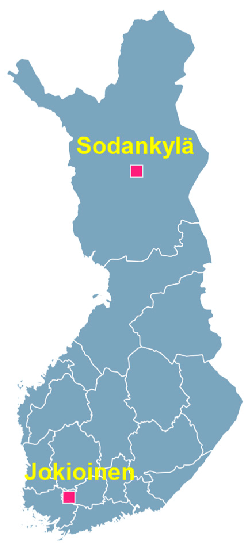
2.1. Stations
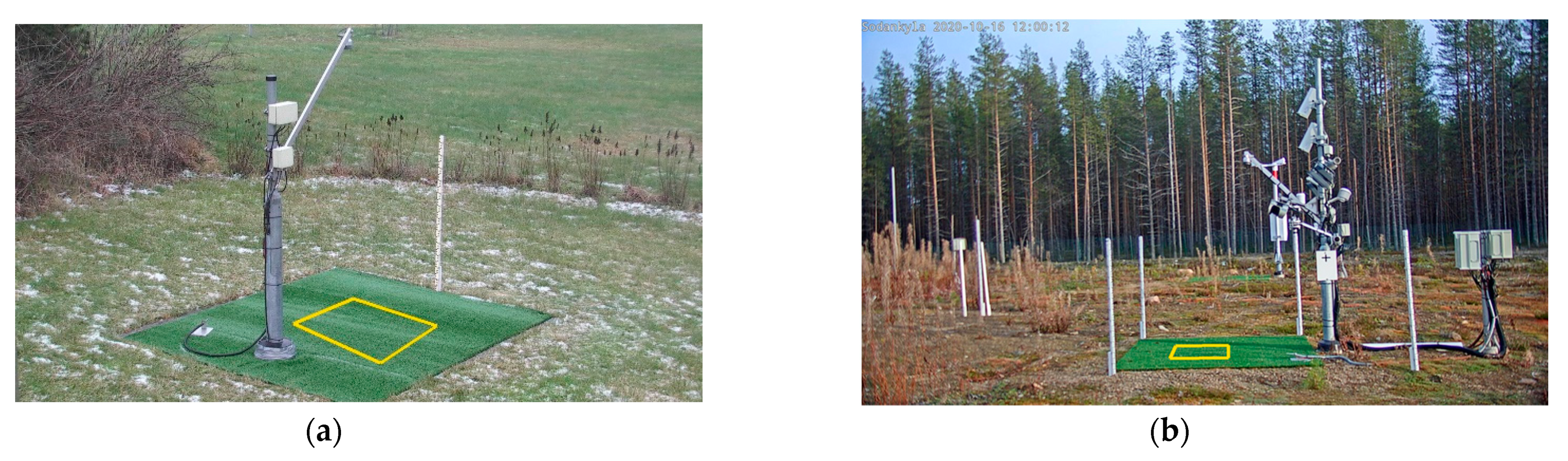
2.1.1. Jokioinen
2.1.2. Sodankylä
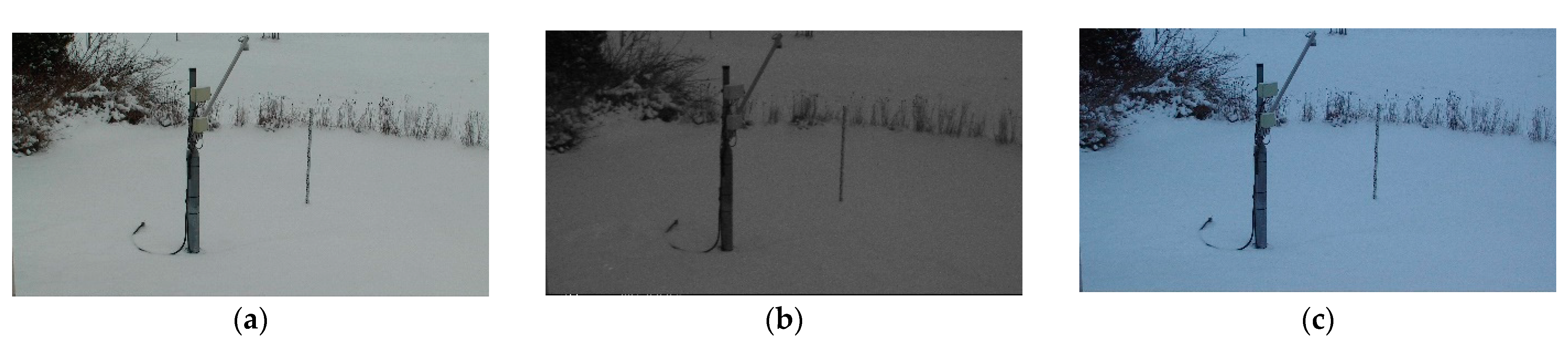
2.2. Camera Imagery
2.3. Ultrasonic Sensors and Snowbed Area
2.4. Visual Inspections
2.5. Estimating FSC from Digital Imagery
2.6. Cloud-Based NRT Processing
2.7. Comparison of FSC from Camera Imagery vs. Visual Inspection
2.8. Comparison of FSC from Camera Imagery vs. SD from US
- SD < 15 mm → SD = 0 mm
- 15 mm ≤ SD < 25 mm → SD = 20 mm
- SD > 20 mm → 5 mm accuracy, e.g.,
- 24 mm rounded to 20 mm.
- 25 mm rounded to 30 mm.
2.9. Assessment of Conditions Where Snow Cover Information Is Fit for Use
2.10. Pilot the Transmission of the FMIPROT Information for the Future Operative Use
3. Results
3.1. Comparison of FSC from Camera Imagery vs. Visual Inspection
3.2. Comparison of FSC from Camera Imagery vs. SD from US
3.3. Validity of FSC When SD from US Is Inaccurate
4. Discussion
Author Contributions
Funding
Data Availability Statement
Acknowledgments
Conflicts of Interest
References
- Pirazzini, R.; Leppänen, L.; Picard, G.; Lopez-Moreno, J.I.; Marty, C.; Macelloni, G.; Kontu, A.; von Lerber, A.; Tanis, C.M.; Schneebeli, M.; et al. European In-Situ Snow Measurements: Practices and Purposes. Sensors 2018, 18, 2016. [Google Scholar] [CrossRef] [PubMed] [Green Version]
- Bongio, M.; Arslan, A.N.; Tanis, C.M.; De Michele, C. Snow depth time series retrieval by time-lapse photography: Finnish and Italian case studies. Cryosphere 2021, 15, 369–387. [Google Scholar] [CrossRef]
- Salvatori, R.; Plini, P.; Giusto, M.; Valt, M.; Salzano, R.; Montagnoli, M.; Cagnati, A.; Crepaz, G.; Sigismondi, D. Snow cover monitoring with images from digital camera systems. Ital. J. Remote Sens. 2011, 43, 137–145. [Google Scholar] [CrossRef]
- Arslan, A.N.; Tanis, C.M.; Metsämäki, S.; Aurela, M.; Böttcher, K.; Linkosalmi, M.; Peltoniemi, M. Automated Webcam Monitoring of Fractional Snow Cover in Northern Boreal Conditions. Geosciences 2017, 7, 55. [Google Scholar] [CrossRef] [Green Version]
- Tanis, C.M.; Peltoniemi, M.; Linkosalmi, M.; Aurela, M.; Böttcher, K.; Manninen, T.; Arslan, A.N. A System for Acquisition, Processing and Visualization of Image Time Series from Multiple Camera Networks. Data 2018, 3, 23. [Google Scholar] [CrossRef] [Green Version]
- Jokinen, P.; Pirinen, P.; Kaukoranta, J.P.; Kangas, A.; Alenius, P.; Eriksson, P.; Johansson, M.; Wilkman, S. Tilastoja Suomen Ilmastosta ja Merestä 1991–2020; Finnish Meteorological Institute: Helsinki, Finland, 2021; Volume 8. [Google Scholar] [CrossRef]
- Nitu, R.; Roulet, Y.A.; Wolff, M.; Earle, M.E.; Reverdin, A.; Smith, C.D.; Kochendorfer, J.; Morin, S.; Rasmussen, R.; Wong, K.; et al. WMO Solid Precipitation Intercomparison Experiment (SPICE) (2012–2015); World Meteorological Organization: Geneva, Switzerland, 2019; Available online: http://hdl.handle.net/20.500.11765/10839 (accessed on 13 February 2023).
- Guide to Instruments and Methods of Observation, Volume I—Measurement of Meteorological Variables, 2018 Edition; World Meteorological Organization: Geneva, Switzerland, 2018; pp. 21–26.
- Lakkala, K.; Jaros, A.; Aurela, M.; Tuovinen, J.-P.; Kivi, R.; Suokanerva, H.; Karhu, J.M.; Laurila, T. Radiation measurements at the Pallas-Sodankylä Global Atmosphere Watch station—Diurnal and seasonal cycles of ultraviolet, global and photosynthetically-active radiation. Boreal Environ. Res. 2016, 21, 427–444. Available online: http://hdl.handle.net/10138/225785 (accessed on 13 February 2023).
- SR50A/AT Sonic Ranging Sensor: User Manual; Campbell Scientific Ltd.: Loughborough, UK, 2011; p. 2.


| Snow Presence | FSC | |
|---|---|---|
| Category | Label | Percent |
| 0 | NULL (e.g., unclear picture) | - |
| 1 | no snow | 0–10 |
| 2 | ground partly covered by snow | 10 < FSC < 90 |
| 3 | full snow cover | 90–100 |
| 4 | frost or ice | - |
| 17.10.2020–4.12.2020 Beginning Season | 4.12.2020–1.4.2021 Winter Season | 1.4.2021–18.5.2021 Melting Season | |||||||
|---|---|---|---|---|---|---|---|---|---|
| Visual Ins. Category | FSC Cat. 1 | FSC Cat. 2 | FSC Cat. 3 | FSC Cat. 1 | FSC Cat. 2 | FSC Cat. 3 | FSC Cat. 1 | FSC Cat. 2 | FSC Cat. 3 |
| 0 | 0 | 0 | 0 | 0 | 0 | 0 | 0 | 0 | 0 |
| 1 | 0 | 0 | 0 | 0 | 0 | 0 | 1 | 1 | 0 |
| 2 | 0 | 0 | 7 | 0 | 0 | 0 | 21 | 107 | 81 |
| 3 | 3 | 3 | 62 | 35 | 145 | 647 | 1 | 58 | 266 |
| 25.12.2020–13.1.2021 Beginning Season | 14.1.2021–1.3.2021 Winter Season | 1.3.2021–15.4.2021 Melting Season | |||||||
|---|---|---|---|---|---|---|---|---|---|
| Visual Ins. Category | FSC Cat. 1 | FSC Cat. 2 | FSC Cat. 3 | FSC Cat. 1 | FSC Cat. 2 | FSC Cat. 3 | FSC Cat. 1 | FSC Cat. 2 | FSC Cat. 3 |
| 0 | 0 | 0 | 1 | 0 | 0 | 0 | 1 | 0 | 0 |
| 1 | 0 | 0 | 0 | 0 | 0 | 0 | 30 | 17 | 0 |
| 2 | 1 | 0 | 27 | 0 | 0 | 0 | 46 | 72 | 37 |
| 3 | 10 | 3 | 36 | 73 | 0 | 184 | 0 | 1 | 37 |
| Observation Site | Snow Season | Number of Obs. | FSC = 0% SD ≥ 15 mm %/Cases | FSC ≤ 10% SD ≥ 15 mm %/Cases | FSC > 0% SD < 15 mm %/Cases | FSC > 10% SD < 15 mm %/Cases | Contradictory Cases/ Day (Based on Days/Season) |
|---|---|---|---|---|---|---|---|
| Sodankylä | melting 2020 (16 days) | 147 | 0.7/1 | 0.7/1 | 29.9/44 | 23.1/34 | 3.0 |
| Sodankylä | beginning 2020 (49 days) | 192 | 1.0/2 | 2.1/4 | 2.6/5 | 2.6/5 | 0.2 |
| Sodankylä | winter 2020–2021 (119 days) | 827 | 0.0/6 | 0.1/17 | 0.0/0 | 0.0/0 | 0.1 |
| Sodankylä | melting 2021 (48 days) | 536 | 0.7/4 | 1.5/8 | 20.0/107 | 15.1/81 | 2.3 |
| Jokioinen | beginning 2020 (20 days) | 75 | 5.3/4 | 5.3/4 | 2.6/2 | 2.6/2 | 0.3 |
| Jokioinen | winter 2020–2021 (47 days) | 257 | 17.9/46 | 17.9/46 | 0.0/0 | 0.0/0 | 1.0 |
| Jokioinen | melting 2021 (46 days) | 241 | 1.2/3 | 1.2/3 | 56.0/135 | 37.3/93 | 3.0 |
| Observation Site | Snow Season | Number of Obs. | FSC > TH% SD < 15 mm V = 1 (False Positive) %/Cases TH = 0 TH = 10 | FSC > TH% SD < 15 mm V = 2 or 3 (True Positive) %/Cases TH = 0 TH = 10 | FSC ≤ TH% SD < 15 mm V = 1 (True Negative) %/Cases TH = 0T H = 10 | FSC ≤ TH% SD < 15 mm V = 2 or 3 (False Negative) %/Cases TH = 0 TH = 10 | Detection Accuracy When SD < 15 mm % TH = 0 TH = 10 |
|---|---|---|---|---|---|---|---|
| Sodankylä | melting 2020 (16 days) | 147 | 1.4/2 0.7/1 | 28.6/42 22.4/33 | 1.4/2 2.0/3 | 0.7/1 6.8/10 | 93.6 76.6 |
| Sodankylä | beginning 2020 (23 days) | 75 | 0.0/0 0.0/0 | 0.0/0 0.0/0 | 0.0/0 0.0/0 | 0.0/0 0.0/0 | N/A N/A |
| Sodankylä | winter 2020–2021 (119 days) | 827 | 0.0/0 0.0/0 | 0.0/0 0.0/0 | 0.0/0 0.0/0 | 0.0/0 0.0/0 | N/A N/A |
| Sodankylä | melting 2021 (48 days) | 536 | 0.4/2 0.2/1 | 19.6/105 14.9/80 | 0.0/0 0.2/1 | 0.9/5 5.6/30 | 93.8 72.3 |
| Sodankylä | All | 1585 | 0.3/4 0.1/2 | 9.3/147 7.1/113 | 0.1/2 0.3/4 | 0.4/6 2.5/40 | 93.7 73.6 |
| Jokioinen | beginning 2020 (20 days) | 75 | 0.0/0 0.0/0 | 1.3/1 1.3/1 | 0.0/0 0.0/0 | 5.3/4 5.3/4 | 20.0 20.0 |
| Jokioinen | winter 2020–2021 (47 days) | 257 | 0.0/0 0.0/0 | 0.0/0 0.0/0 | 0.0/0 0.0/0 | 17.9/46 17.9/46 | 0.0 0.0 |
| Jokioinen | melting 2021 (46 days) | 241 | 15.6/37 9.3/22 | 40.9/97 29.5/70 | 4.1/10 10.4/25 | 1.2/3 1.2/3 | 72.8 79.2 |
| Jokioinen | All | 573 | 6.5/37 3.8/22 | 17.1/98 12.4/71 | 1.7/10 4.2/24 | 9.2/53 9.2/53 | 54.5 55.9 |
| All | melting combined | 924 | 4.4/41 2.6/24 | 26.4/244 19.8/183 | 1.3/12 3.1/29 | 1.0/9 4.7/43 | 83.7 76.0 |
| All | All | 2158 | 1.9/41 1.1/24 | 11.4/245 8.5/184 | 0.6/12 1.3/28 | 2.7/59 4.3/93 | 72.0 64.4 |
Disclaimer/Publisher’s Note: The statements, opinions and data contained in all publications are solely those of the individual author(s) and contributor(s) and not of MDPI and/or the editor(s). MDPI and/or the editor(s) disclaim responsibility for any injury to people or property resulting from any ideas, methods, instructions or products referred to in the content. |
© 2023 by the authors. Licensee MDPI, Basel, Switzerland. This article is an open access article distributed under the terms and conditions of the Creative Commons Attribution (CC BY) license (https://creativecommons.org/licenses/by/4.0/).
Share and Cite
Tanis, C.M.; Lindgren, E.; Frey, A.; Latva, L.; Arslan, A.N.; Luojus, K. Use of Webcams in Support of Operational Snow Monitoring. Geosciences 2023, 13, 92. https://doi.org/10.3390/geosciences13030092
Tanis CM, Lindgren E, Frey A, Latva L, Arslan AN, Luojus K. Use of Webcams in Support of Operational Snow Monitoring. Geosciences. 2023; 13(3):92. https://doi.org/10.3390/geosciences13030092
Chicago/Turabian StyleTanis, Cemal Melih, Elisa Lindgren, Anna Frey, Lasse Latva, Ali Nadir Arslan, and Kari Luojus. 2023. "Use of Webcams in Support of Operational Snow Monitoring" Geosciences 13, no. 3: 92. https://doi.org/10.3390/geosciences13030092