1. Introduction
Snow is a vital component of the hydrological cycle in many mountainous snow-dominated basins where glaciers and seasonal snowpacks are the water supplier of more than 1/6 of the Earth’s population [
1]. Proper estimation of hydrological response in these regions is crucial for the effective operation of the upstream reservoirs which function for hydropower, irrigation, and water supply. To that end, hydrological forecasting systems have been developed and applied for many decades. However, their representations are still challenging due to the complexities associated with snow accumulation and melting processes, the limitation of data availability in rough topography, and harsh weather conditions.
In order to improve the performances, hydrological forecasting for snow-dominated regions in literature copes with different aspects such as accounting for numerical weather prediction data [
2,
3,
4], implementing different type of observations [
5,
6,
7,
8,
9,
10], and applying varying model approaches [
11,
12,
13,
14,
15]. Observing snow by in situ measurements is traditional with ground-based meteorological networks. Still, it is challenging to have spatial variability and to access upper zones where snow cover stands for a more extended period [
16]. Snow physics and harsh topography force modelers to employ advanced satellite and remote sensing tools to detect snow, such as Snow Cover Area (SCA) and Snow Water Equivalent (SWE) [
17,
18].
Model results in hydrological forecasting are not perfect due to uncertainties such as model input data, initial conditions, model structure, and parametrization [
19,
20,
21]. To overcome these uncertainties, forecasting systems are subjected to several improvements. For example, forcing uncertainty may be coupled with ensemble numerical weather predictions [
2] or integrating probabilistic approaches [
22]. Data assimilation methods are useful techniques in many disciplines that help model developers decrease uncertainties by updating the model states and improving initial conditions. Data assimilation approaches are the most common way (often a prerequisite for forecasting) of adapting the observed information into the model to improve initial conditions [
6,
23,
24,
25,
26].
Researchers have shown the advantages of including snow data in hydrological modeling studies for calibration and validation of degree-day based conceptual models [
27]. Optimization of model parameters during calibration may force the model to compensate for rainfall-runoff error while sacrificing snow components. Data assimilation could increase the parsimony of the snow states, however, most of the existing implementations of data assimilation in hydrological forecasting have focused on the assimilation of streamflow. The model states which cannot be directly measured become more robust but still suffer from poor snow states and snow forecasts as the external output from the model itself. This is because the assimilation of snow data (SCA, SWE, or snow depth) is not as straightforward as compared to streamflow data. However, the integration of remote sensing snow data and ground snow measurements into data assimilation applications for an operational system is a relatively new field of research which is receiving growing attention [
7,
28,
29,
30,
31,
32]. This might be even more crucial for data-sparse snow-dominated regions; thus, studying and practicing data assimilation techniques with snow observations contributes to a better representation of models.
On the other hand, accounting for the uncertainty of the model structure (due to parametric and structural uncertainty) is very important since the parameters are generally calibrated and validated for a particular part of the selected historical period. Often, model sensitivity analysis provides useful information to detect the degree of uncertainty [
33]. Additionally, this type of uncertainty can be reduced by using multi-modelling methods [
2,
34,
35,
36].
Data assimilation methods are mainly categorized into: (i) filtering approaches and (ii) smoothing approaches. The filtering approach (Extended Kalman Filter, Ensemble Kalman Filter, Particle Filter, etc.) is one of the most widely used way of updating states since it does not require adjoint modeling and is easy to implement [
37]. In the smoothing approach, updates are done simultaneously over multiple time steps and they can be advantageous in handling time lags between observations and updated states. Variational Data Assimilation (VarDA) is a smoothing type of data assimilation implemented together with Moving Horizon Estimation (MHE) in which an objective function is numerically solved using optimization algorithms to obtain an optimum between model and observation uncertainties. It also provides flexible formulation without considering explicit error covariance matrices [
38]. Alvarado et al. [
29] introduced an innovative probabilistic version of VarDA, so-called Multi-Parametric VarDA (MP-VarDA), and showed that the new version provides more robust results compared to the conventional deterministic VarDA by assimilating both streamflow and SCA. The MP-VarDA consists of using multiple model parametric sets with the same model structure in order to create an ensemble of model runs that quantifies model parametric uncertainty. In the MP-VarDA, the noise introduced by the optimization algorithm is common for all model runs. This enables a unique modification of the model pool during the assimilation procedure. The ensemble of model runs, equivalent to the prior estimate in filtering methods, provides an estimate of the model parametric uncertainty. The model parameter sets are obtained from an Aggregated Distance (AD) method which maximizes the parametric distance between each model set in an effort to provide a maximum diversity in the quantification of parametric uncertainty.
This study aims to implement and test this recent method [
29] that generates a probabilistic estimate of initial states using a multi-parametric modelling method. This study also tests the MP-VarDA method for the first time in a data-scarce snow-dominated region and the performances of the snow outputs are separately analyzed. Apart from that, according to the authors’ knowledge, the appropriate model pool number selection in MP-VarDA has not been tested in any study so far. Therefore, the main innovation of this study is to reveal the sensitivity of the number of models in a model pool using the MP-VarDA method coupled in the HBV model that is needed to capture model dynamics in data assimilation and compare it with its deterministic counterpart (VarDA).
Karasu catchment is a pilot basin for many national and international projects, with a high snowmelt contribution of around 60–70% in annual streamflow volume. Concerning the importance of snow in mountainous Eastern Türkiye and the limited availability of data, incorporating different data assimilation techniques with various snow data sources is crucial in the region’s streamflow predictions. Considering these, the companion paper discusses the conceptual hydrological model (HBV) with variational and sequential data assimilation techniques using satellite snow products as a case study in the Upper Euphrates Basin (Karasu), Türkiye and in the Canales Basin, Spain [
28]. However, the uncertainties associated with model parametrization and their consideration in data assimilation techniques are still research questions for forecasting systems.
This study is also conducted in mountainous Eastern Türkiye for streamflow predictions over the region concerning the importance of snowmelt and the limited data availability. The study aims to clarify the effects of different model pool instances (mpi) in probabilistic variational data assimilation techniques in forecasting streamflow and snow cover area. The study is also valuable by accounting for snow data in assimilation configuration for a snow-dominated region. The objectives of the study are to reveal the value of MP-VarDA, investigate the effect of different model pool instances for capturing the model uncertainty, and finally compare the probabilistic MP-VarDA performances with deterministic VarDA.
2. Materials and Methods
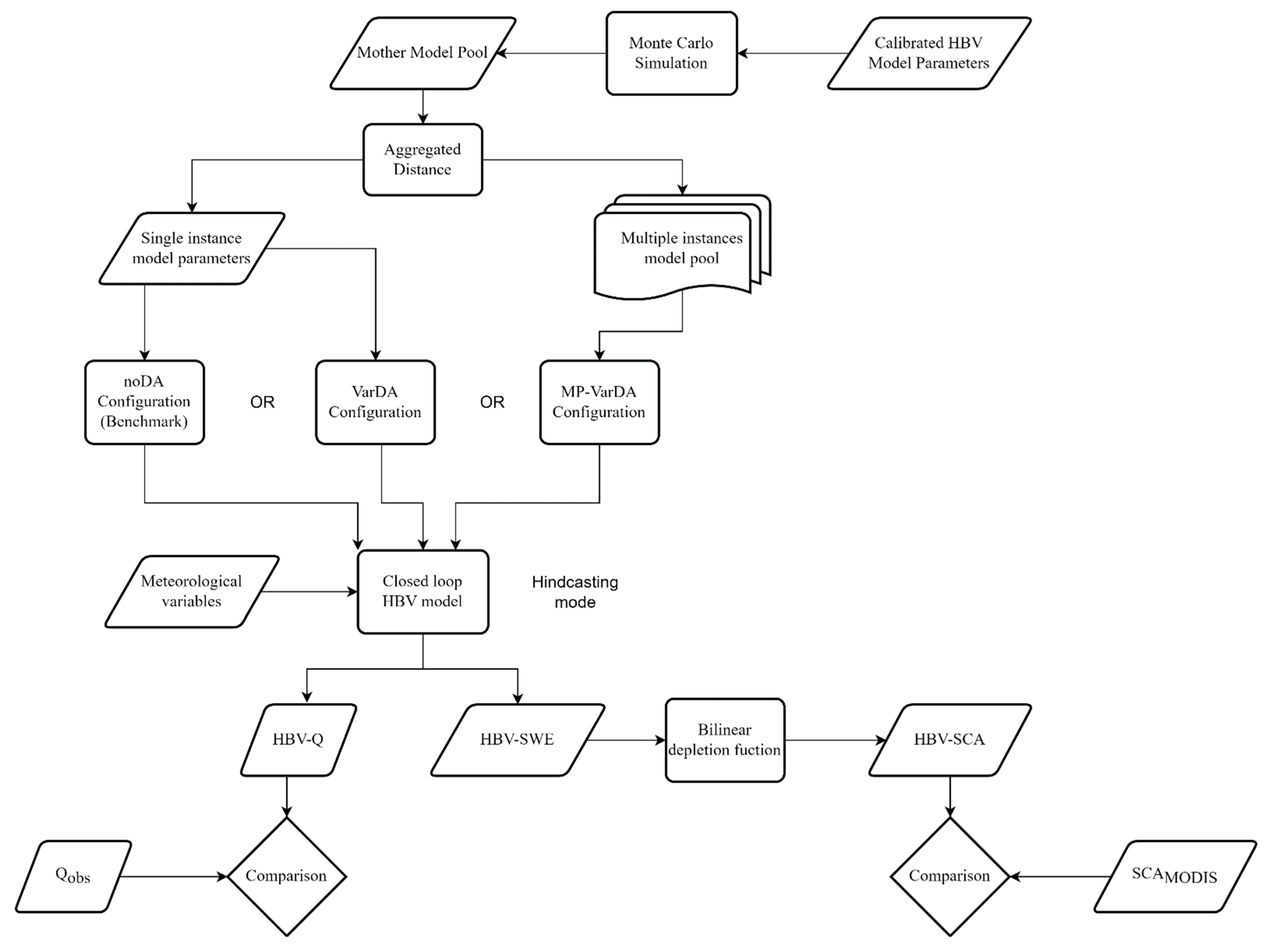
A flowchart is presented in
Figure 1 to demonstrate the methodology of the study. The daily rainfall-runoff relationship is established under the HBV model. The model has 21 parameters to mimic the streamflow observed at the outlet of the basin. The details of the hydrological model are given under
Section 2.3. The structural uncertainty is represented by multiple model instances. To that end, the Monte Carlo simulation creates multiple model parameter sets (so-called mother model pool) around the previously calibrated and validated single model parameter set of the HBV model. Since it is not practical to use all parameterization, AD method was utilized to reduce the number of the model parameter instances. The reduced parameters are mainly split into two categories: (i) single instance model parameters and (ii) multiple instance model pool parameters.
The uncertainties of the initial conditions were tackled with the variational data assimilation technique. The benchmark simulation (noDA configuration) enables the detection of any gain obtained from the data assimilation implementation. The configuration of the assimilation accounts for perturbations over state forcings and observations. Conventional deterministic VarDA is also implemented using a single instance model parameter set. A multiple instance model pool is composed of various sets depending on the number of the instances such as 3, 5, etc. The HBV model is run within a hindcast period, and the comparisons of both techniques, together with the benchmark case, are demonstrated. The forecasts are produced as a set of ensembles for the MP-VarDA method. This is similar to data assimilation based hydrological ensemble forecasting done by numerical weather forecasts, but here forecast members are generated using multi-parametrization and different probabilistic initial conditions, which is different than producing ensemble members using ensemble forcing data into a single hydrologic model and the same initial conditions.
The HBV model produces both streamflow and SWE forecast outputs. In this study, HBV-based SWE values were converted to SCA. The data assimilation implementation also accounted for the assimilation of both observations (streamflow (Q) and SCA). Therefore, the outputs (HBV-Q and HBV-SCA) are also compared with the observation (observed streamflow and satellite SCA) using verification metrics. The study was conducted during the 2009–2012 Water Years (WYs), which are the 12 months between 1 October and 30 September in Türkiye.
2.1. Study Area and Hydro-Meteorological Data
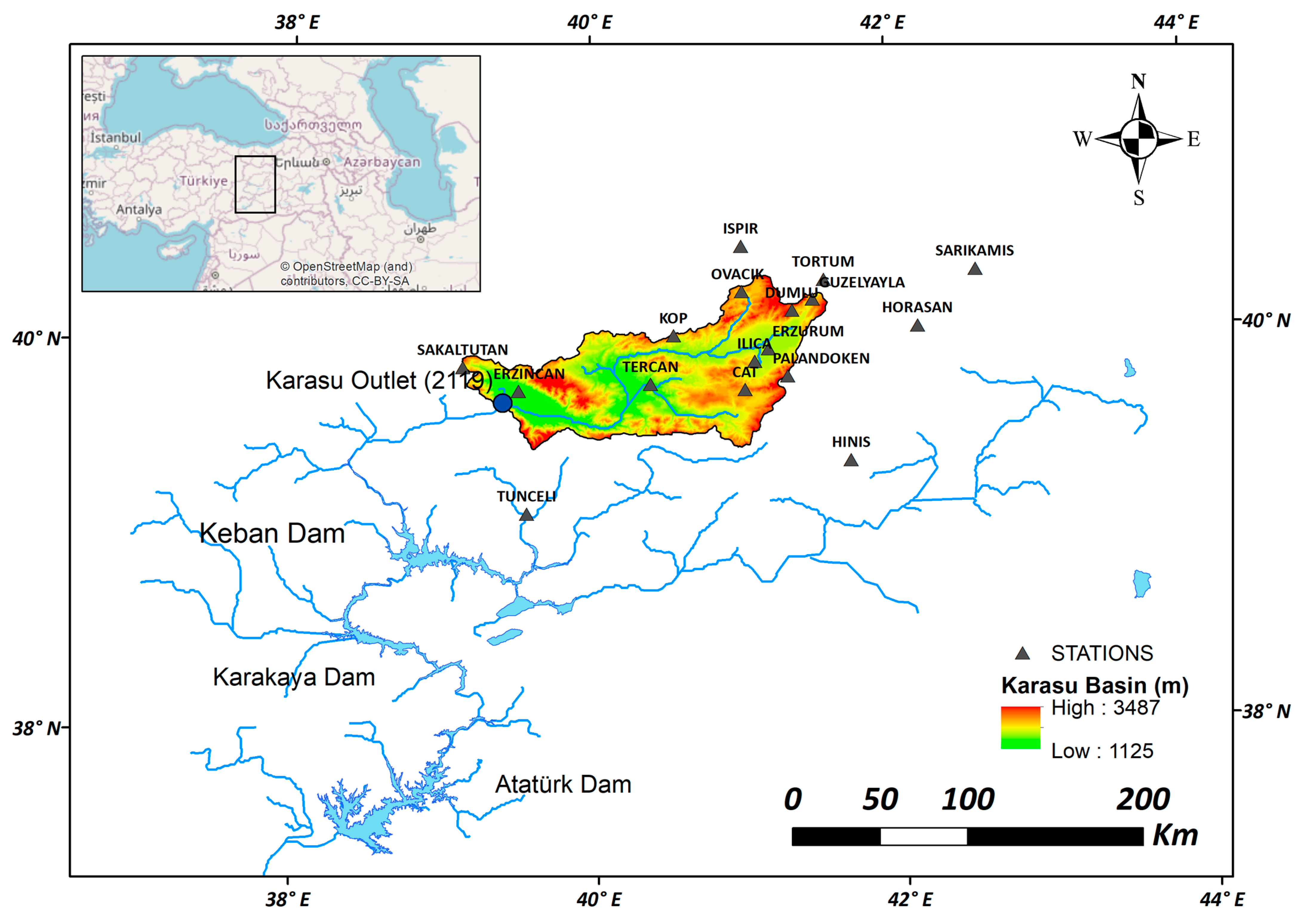
The developed methodology was tested in the Karasu River catchment, a major branch of the Euphrates River in Türkiye. The study area and station network are shown in
Figure 2. The basin with a drainage area of 10,275 km
2 has an elevation range from 1125 m to 3500 m and a hypsometric mean elevation of 1983 m. The main land cover types are pasture, cultivated, and bare land. Snowmelt streamflow in the mountainous eastern part of Türkiye is of great importance. It constitutes approximately two-thirds of the volume of the total yearly streamflow during the spring and early summer months. The streamflow data were collected at the outlet of the basin (2119 station). Karasu Basin is divided into 10 elevation zones (bands) between 1125–3500 m. A total of 18 climatologic and automated weather operating stations (AWOS), ranging in elevation between 981 and 2937 m, are located in and around the basin (
Figure 2). The required input data for the HBV model are daily total Precipitation (P), daily average Temperature (T), and daily Potential Evaporation (PE). In this study, input data are provided as zone-based areal values calculated by the Detrended Kriging distribution method [
39].
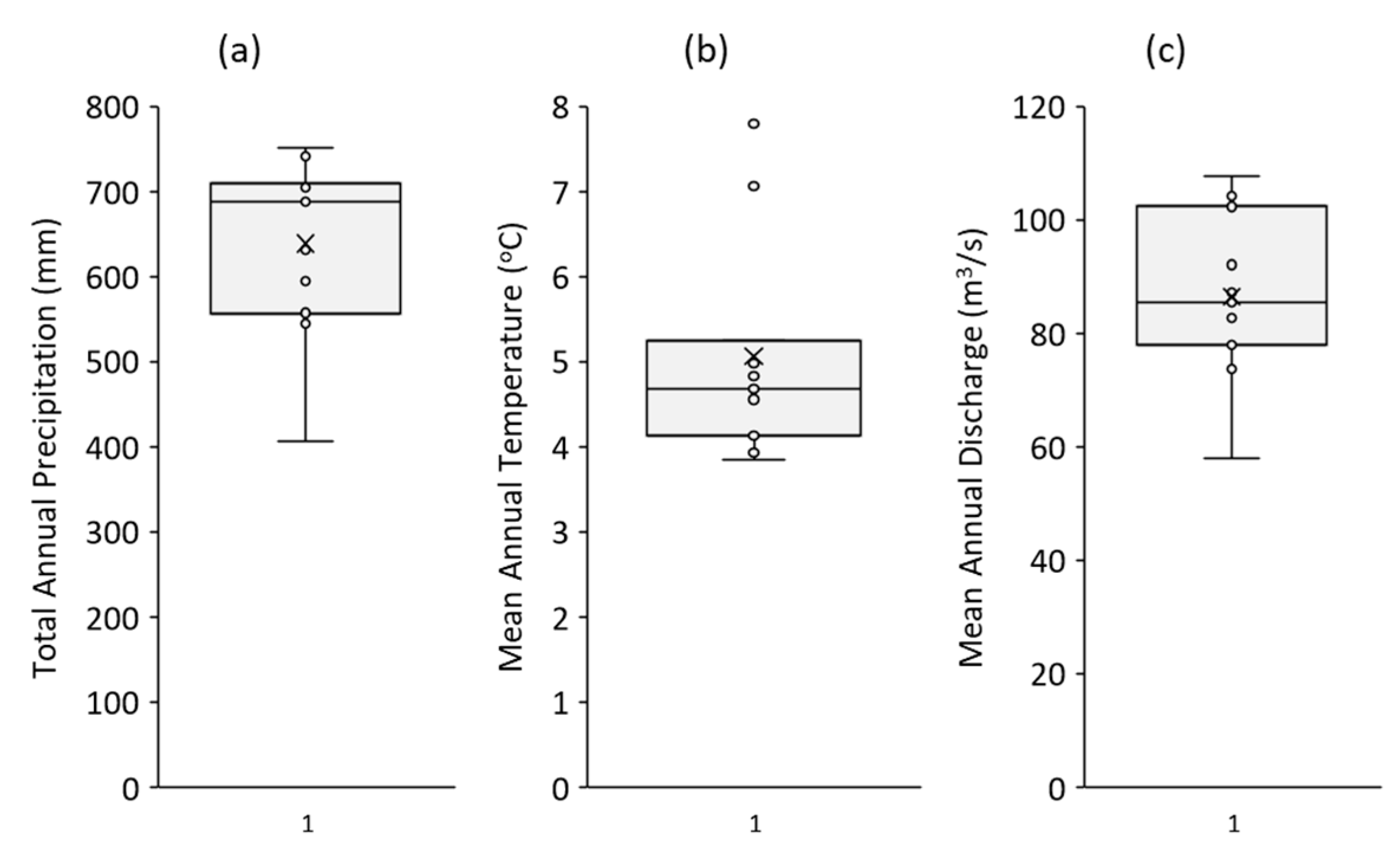
The box and whisker plots of the hydro-climatic data (total annual P, average annual T and the mean annual streamflow) are given in
Figure 3. In summary, the overall basin statistics are observed for the mean total P, and the mean annual temperature and the mean annual streamflow are 638 mm/year, 5.1 °C, 86 m
3/s, respectively.
2.2. Snow Cover Area (SCA) Data
In snowmelt streamflow modeling, it is essential to either use snow data as input to the model or validate the model output with observations. In this study, snow data were calculated from Moderate Resolution Imaging Spectroradiometer (MODIS) observations. The MODIS snow-mapping algorithm is fully automated and is based on the Normalized Difference Snow Index (NDSI) in a set of thresholds [
40]. However, optical satellites like MODIS are suffering from cloud coverage, especially during the snow season, resulting in missing areal SCA data for cloudy days. In this study, cloud-free SCA data are provided by certain filters such as combination, temporal, spatial, and elevation [
41]. Therefore, filtering enables continuous cloud-free observations of MODIS SCA data over the Karasu catchment.
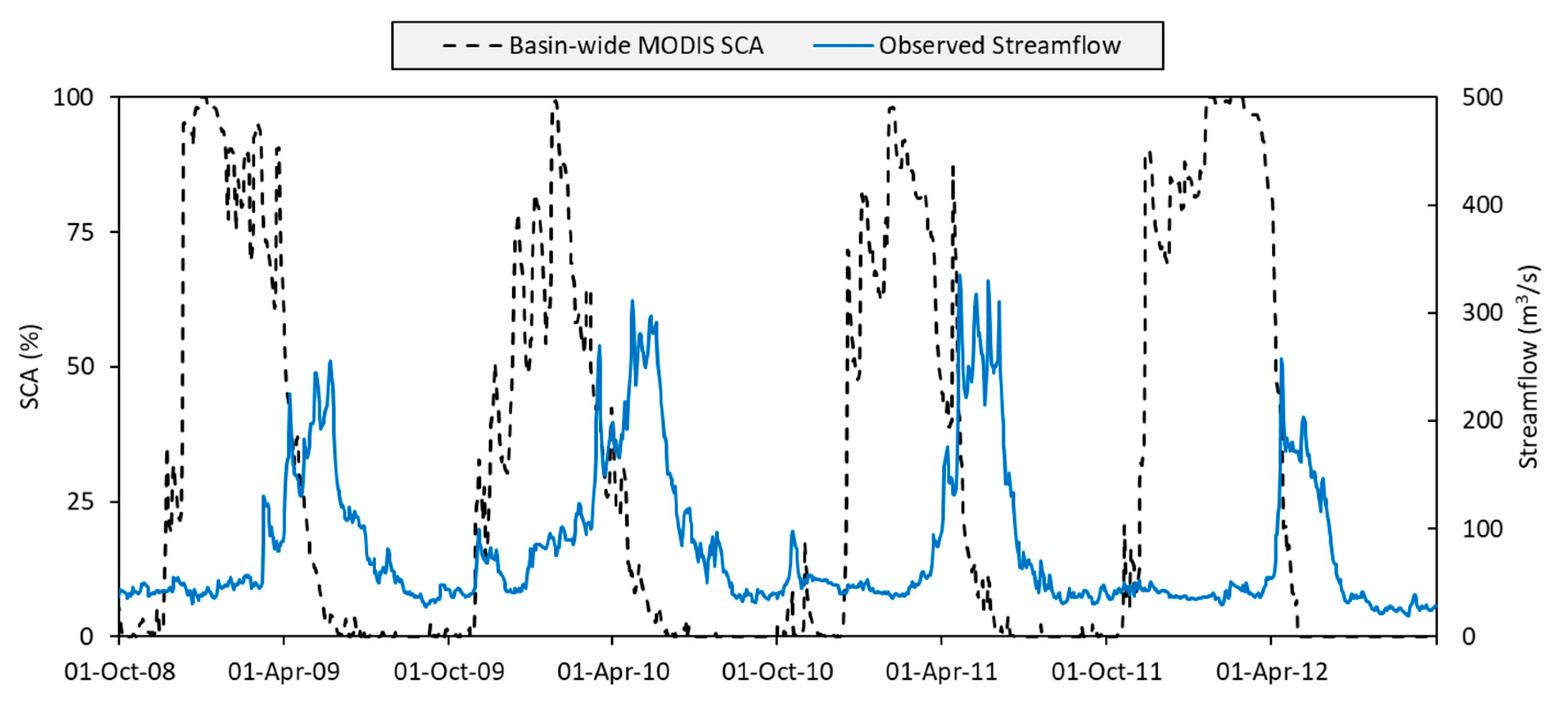
Observed daily SCA data were converted to daily time series for each elevational zone for the study period. HBV model produces SWE, converts it to SCA, and utilizes the observed SCA information for the data assimilation part.
Figure 4 depicts the variation of SCA of the whole catchment and streamflow at the outlet of the basin for the 2009–2012 WY period. During the accumulation period, the streamflow values are low while the major portion comes during and after the start of the melting season. Besides, remote sensing snow products (MODIS, IMS, MSG-SEVIRI) provide above 90% accuracy with ground measurements in the region [
41,
42,
43,
44].
2.3. HBV Hydrological Model
HBV model is a bucket-type, semi-distributed conceptual model to employ the hydrological processes by dividing a hydrological basin into sub-basins and/or elevation ranges [
45]. The model generally consists of three main routines as: snow, soil moisture and runoff response. HBV simulates the rainfall-runoff relationship using the degree-day method in mountainous regions. Our dedicated implementation of the HBV model is documented in Schwanenberg and Bernhard [
46] and refers to Bergström [
47] and Lindström et al. [
48]. For this study, the variational data assimilation (VarDA) approach is based on the Moving Horizon Estimation (MHE) formulation defined in [
29]. Therein, the hydrological model can be described in a time discretization according to:
where
,
, and
are the state, output, and external forcing vectors, respectively,
,
are noise terms,
is the model parameters (see Abbreviation for the definition of each parameter) vector,
and
are functions representing arbitrary linear or non-linear components of the model, and
is the time step index.
The model takes daily total P, daily average T and PE as main inputs and produces modelled outflow. In the HBV model application structure, the basin is divided into ten elevation zones with equal areas. The accumulated streamflow of these elevation zones contributes to modeled outflow, which is compared to the measured streamflow at the outlet streamflow gaging station of the basin (2119 station). The model was chosen to operate on an open area land use along with daily time steps. The model also produces SWE as the model state. A simple bilinear function converts the SWE computed by the model to SCA. Modelled SCA is also compared with observed SCA provided by MODIS snow product.
The model has 21 parameters, including the Muskingum routing parameter, and was calibrated using the interior point algorithm Ipopt [
49]. The calibration was done for the water years 2002–2008, resulting in a Nash–Sutcliffe Efficiency (NSE) performance of 0.84. The calibrated parameters were validated for 2009–2012, which resulted in a NSE of 0.70.
2.4. Deterministic and Multi-Parametric Variational Data Assimilation
A deterministic VarDA approach was conducted for a forecast time
over an assimilation period
of
time steps by the optimization of an objective function
according to Equation (3) and was subject to Equations (4) and (5):
where
and
are observations of the state and the dependent variable vectors, respectively,
,
,
are weighting coefficients to define the trade-off between different penalties,
is a suitable norm penalizing the deviation between observed and simulated quantities as well as the amount of noise introduced by the data assimilation procedure. Note that the optimization setup modifies the noise variables
and
to find the minimum value of the objective function. Furthermore, the noise terms get bounded by inequality constraints which consider constant lower and upper bounds during the complete assimilation period.
Multi-parametric variational data assimilation, MP-VarDA, is an extended version of deterministic Moving Horizon Estimation-based VarDA described above in Equations (3)–(5). The main difference is that MP-VarDA assimilates information into a pool of
number of model instances, according to Equation (6), and subject to Equations (7) and (8). In this study, the probability
for each model is defined as equally likely. The amount of noise introduced to the system is equally distributed among all
models.
The Monte Carlo simulation technique was used to create multiple model parameters based on a previously calibrated hydrological model. The idea is that very different parameter sets can yield almost equally good fits between simulated and observed streamflow. The simulations are bounded by a multiplicative factor concerning the calibrated set as well as a physical limit such that:
where
is the parameter
of the calibrated set,
is a variation factor, and
is the modified parameter bounded to the lower and upper bounds
and
respectively. The parameters
were generated using the Monte Carlo method.
The multiple model parameters include a large set, but it is not practical to implement all of them in MP-VarDA due to its computational expense. Therefore, we aimed at producing a representative set of models (model pool) from the Monte Carlo simulation. Here, we use the AD method [
29] to reduce the number of parameter sets while still keeping the maximum amount of parametric uncertainty in the remaining sets. Model pool(s) were established from the same multiple parameter set (Monte Carlo simulation runs only once in the entire study), but each pool has varying model instances. The study analyzes the performance of different model pools in MP-VarDA. The model pool with more instances always includes a model pool with fewer instances. For example, a model pool having 5 instances includes model pools 3 and 1. This guarantees the inclusion of the same model uncertainty captured in different larger model pools. On the other hand, the model pool having only one model instance is considered to be representative of VarDA to compare with MP-VarDA results and is similarly created from multiple parameter sets.
Since the variational methods use optimization algorithms to minimize an objective function, the trade-off is done between the amount of noise introduced into the model and the distance between simulated and observed variables. Unlike a single VarDA, MP-VarDA optimizes the function using multiple model instances. Streamflow and snow (satellite SCA) observation data were assimilated using noise terms of states and forcings such as precipitation and temperature, as indicated in
Table 1. The other states (SM, UZ, and LZ) of the HBV model are also accounted for in the objective function. The probabilistic initial values are produced by MP-VarDA, and ensemble forecasts are produced with probabilistic initial states and multi-model structure. The range of noise terms and weight of the observations are given in
Table 1. This configuration is compared with other alternatives and the optimum weights were assessed based on forecast gains in Alvarado-Montero et al. [
28]. The setup assimilates streamflow and snow data; thus, it claims to improve both forecast outputs. Moreover, we kept the assimilation window in both applications up to 6 months to capture a larger time lag between forcings and observations.
2.5. Aggregated Distance (AD) Method
The produced multiple parameter sets by Monte Carlo simulation should be reduced to representative members. There are different reduction approaches (fast forward, random selection, tree-based, etc.) in the literature. The selected algorithm plays a key role since it should capture a significant part of parametric uncertainty. AD is a robust method because it is a distance-based method, so the reduction is subjected to eliminating the parameter set m with the minimum aggregated distances to the rest of the parameter sets. The probability of parameter set m is then reassigned to its closest set. This procedure is repeated until the chosen number of parameter sets R is reached after N − R iterations, where N is the initial number of parameter sets. R is also selected by the user. In this study, the effects of selection R are also assessed, and results are compared. The details of the AD method are described in Alvarado-Montero [
50].
2.6. Monte Carlo Configuration and Model Pool Generation
The VarDA configuration is based on a set of calibrated HBV hydrological model parameters (single model pool). The multiple model parameters
pi,m are generated using the Monte Carlo method based on normal distribution perturbation around the previously calibrated parameters. To that end,
Fvar (Equation (9)) is set to 30% and the number of the simulations are selected as 1000 under the Monte Carlo method. The parameter sets (mpi1000) produced by the Monte Carlo method were subjected to the performance threshold (with model performance above 98% of the calibrated model). Among them, only 800 sets (mpi800) satisfies this threshold. It is not practical to account 800 mpi in the MP-VarDA method, thus the parameters (mpi800) are reduced to mpi1, mpi3, mpi5, and mpi10 using the AD reduction technique. After reduction, each mpi is implemented in a hindcasting (closed-loop) mode and represents an experiment, as given in
Table 2. The benchmark NoDA and deterministic VarDA stand for mpi1, whereas the others (mpi3, mpi5, mpi10) represent probabilistic data assimilation under MP-VarDA configuration.
2.7. Performance Metrics
The study tests the close-loop performances of the forecast system. While the deterministic method (VarDA) based forecasts are single trajectories, the probabilistic data assimilation method (MP-VarDA)-based forecasts have multiple members (ensemble). The number of the ensemble is equal to the number of mpi, i.e., probDA-mpi3 produces three different forecasts in each time step up to the lead time. Therefore, the performance metrics in this study are commonly used statistics in ensemble forecast systems and rely on the Ensemble Verification System (EVS) 5.4 developed by the National Oceanic and Atmospheric Administration, NOAA [
51]. The exceedance probabilities are first calculated for Pr = 0.25, Pr = 0.50, and Pr = 0.75 of the observed data set. Following that, these probabilities were set as the thresholds, and forecasted streamflow and SCA were separately assessed over these thresholds.
The Brier Score (BS) in Equation (11) measures the average square error of a probability forecast. It is equivalent to the mean square error of a deterministic forecast, but the forecasts, and hence error units, are given in probabilities. For an event that involves not exceeding some threshold,
, the BS is computed from the forecast probability,
, and the corresponding observed outcome,
, whose cumulative probability is 1 if t is exceeded by the observation and 0 otherwise, as defined by the step function,
.
The Brier Skill Score (BSS) in Equation (12) measures the performance of one forecasting system relative to another in terms of the Brier Score (BS). The BSS comprises a ratio of the BS for the forecasting system to be evaluated (the “main forecasting system”), BS
MAIN, over the BS for the reference forecasting system, BS
REF. BSS closer to 1 is preferred.
On the other hand, data assimilation accuracy was also attained using mean Continuous Ranked Probability Score (m-CRPS), so Continuous Ranked Probability Score (CRPS) was calculated according to Equation (13). The m-CRPS metric is equivalent to the mean absolute error when using deterministic forecasts. It provides information on the accuracy of the forecast.
where:
represents the value of the forecast
with a leadtime
L,
is the indicator of the forecast,
is the number of ensembles,
is the mean of the ensemble forecast,
is the cumulative distribution function, and
is a function that assumes probability 1 for values higher or equal to the observation and 0 otherwise.
3. Results
3.1. Monte-Carlo Simulation and Model Pool Instance Results
Only around 800 of the total 1000 model instances that had different parametrization were selected, considering performance threshold (with model performance above 98% of the calibrated model). This ensures the reliability of the model sets used in data assimilation application.
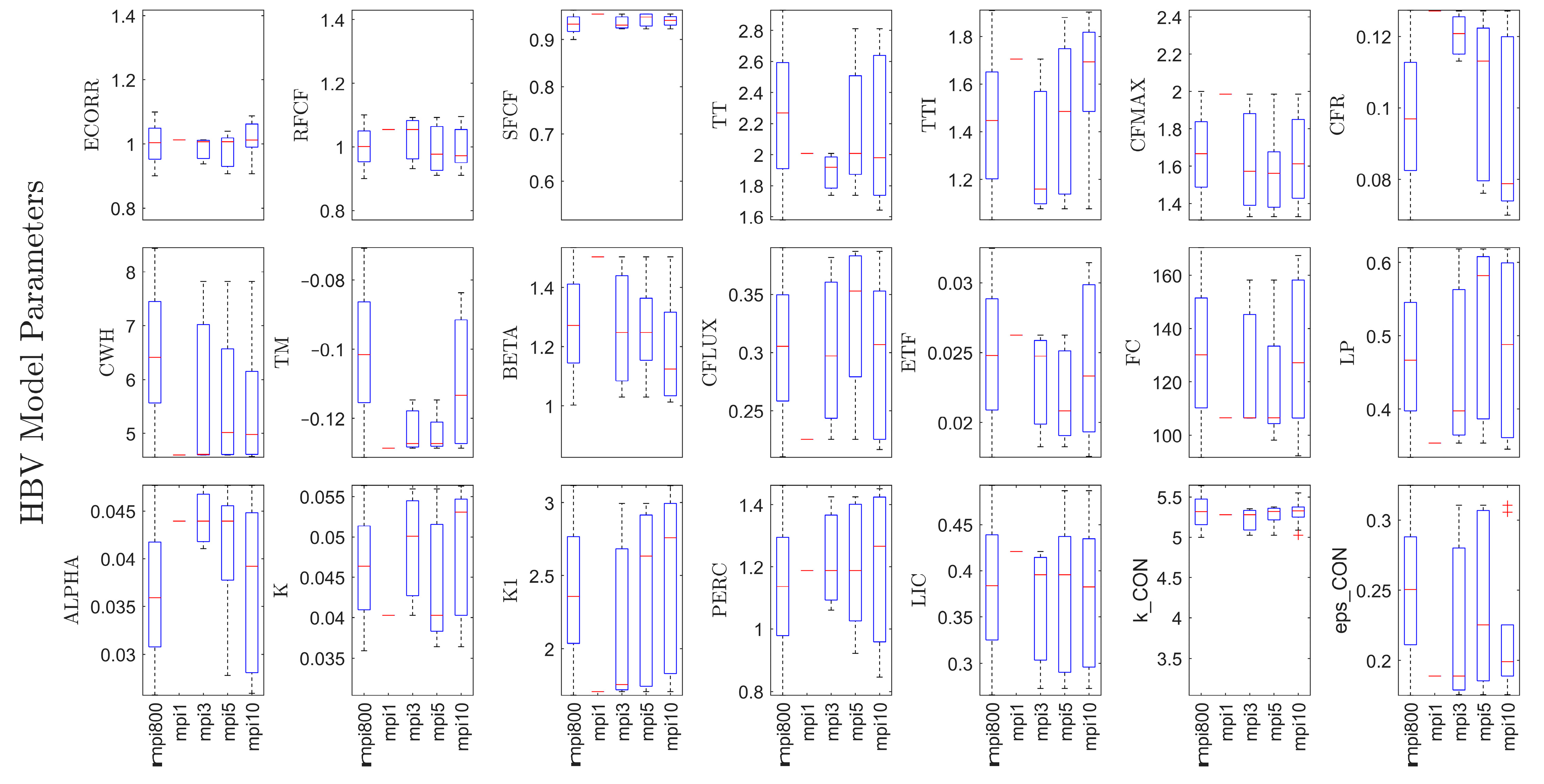
Figure 5 demonstrates the distribution of parameters for each mpi (with box and whisker plots) produced by the Monte Carlo method (both for mpi800 and AD-based reduced mpi). For example, the spread of mpi800 has the highest variation due to its capability of multi-modeling ability. However, the idea here is to demonstrate the variation of the deterministic (mpi1) and reduced probabilistic sets (mpi3, mpi5, and mpi10) in comparison with mother pool (mpi800). The upper and lower y-axis limits of the graph are adjusted according to the physical limits of the parameters.
Table 3 shows the ranges of the mother pool set categorized into three groups depending on the visual parameter comparison in
Figure 5. Accordingly, only 4 parameters have low-range and 3 parameters are within mid-range, while the remaining total 14 parameters are found to provide a good fit, with the observed streamflow having a wide range.
The Monte Carlo method can capture a more extensive distribution by having larger parameter sets. Since mpi1 has a single member parameter set, it provides a single value in the graph (
Figure 5). Thus, the parameters of mpi1 do not always match the mean of the mother pool (mpi800). However, it can be stated that AD-based model pools show promising distribution, even with fewer model instances: correction factor for evaporation (ECORR), correction factor for rainfall (RFCF), temperature interval with a mixture of snow/rain (TTI), degree day factor (CFMAX). Additionally, increasing the number of the model pool can properly represent a larger spread; see temperature limit for snow (rain or snow) (TT), recession coefficient (ALPHA), and field capacity (FC).
Even the small number of AD-based parametrization can rapidly converge to the mother model pool ranges. For example, this is observed for the parameters of K1, CFMAX, or BETA, where the 1 mpi value is close to the minimum or maximum value of the mother pool, while 3 mpi can rapidly capture the mother pool range. Outliers are only detected in Muskingum routing parameters (k_CON and eps_CON) for the 10 mpi.
3.2. Data Assimilation Hindcast Results
The hindcast period starts from 1 October 2008 and ends on 30 September 2012, and has daily time steps. The forecast lead time is set to 10 days (0 to 240 h with 24 h increments). The initial conditions were improved by assimilating both streamflow and snow data under deterministic and probabilistic variational DA. Improved states were utilized as the best initial condition to generate perfect forecasts based on observed forcing data. This also eliminates forecast uncertainty, which is out of the scope of this study. Generated model pool parameter sets (mpi1, mpi3, mpi5, and mpi10) were implemented into data assimilation through the HBV hydrological model in a hindcasting mode. The configuration intended to produce both streamflow and SCA forecasts. Since VarDA is deterministic, it produces a single forecast for each time step up to the lead time, whereas MP-VarDA produces an ensemble set of forecasts considering multiple initial conditions and model parametrization.
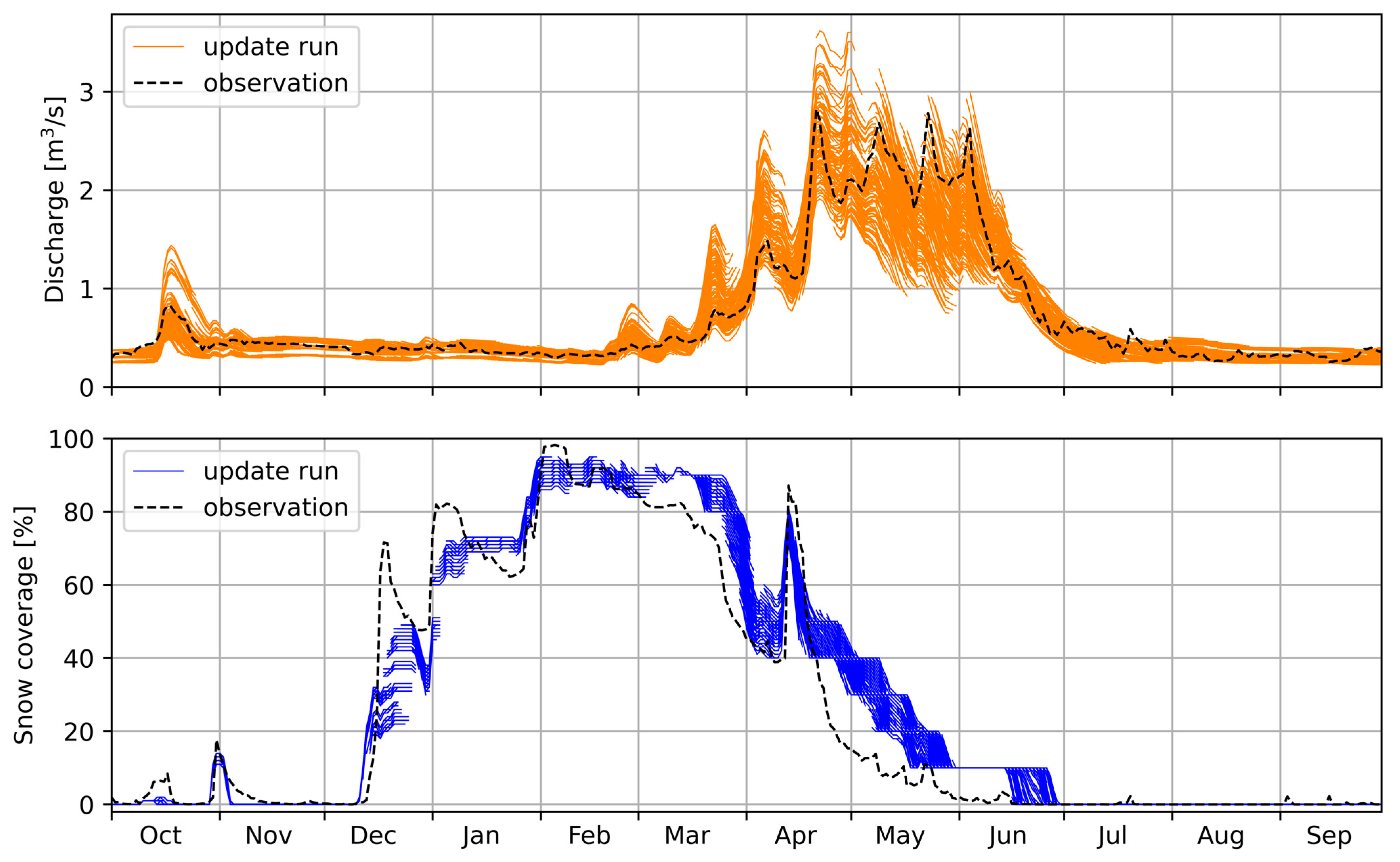
Figure 6 demonstrates the multi-model ensemble forecasts of the probDA-mpi10 experiment as an example case from the 2011 WY by mpi10 parameterization and MP-VarDA application coupled in HBV. The dash lines indicate the streamflow and SCA observations. The orange and blue lines are produced streamflow and SCA forecasts that have 10 members for up to 10-day lead time in daily time step, respectively.
The streamflow thresholds (depending on the exceedance probabilities; Pr = 0.25, Pr = 0.50, Pr = 0.75) from the observations are calculated as 39.5 m3/s, 49.4 m3/s, and 100.4 m3/s, respectively. The SCA thresholds (Pr = 0.25, Pr = 0.50, Pr = 0.75) from satellite observations are calculated as 0.01%, 6.23%, and 69.47%. Thresholds are lower limits for the assessments. Therefore, the forecast members above Pr = 0.25, Pr = 0.50, and Pr = 0.75 for streamflows are deemed as “above low flow”, “above median flow”, and “high flow”, respectively. On the other hand, Pr = 0.25 for SCA encompasses any snow occurrences by excluding summer months, while Pr = 0.50 threshold stands for the accumulation and melting periods, and finally Pr = 0.75 only evaluates the high and full snowy seasons.
Figure 7 and
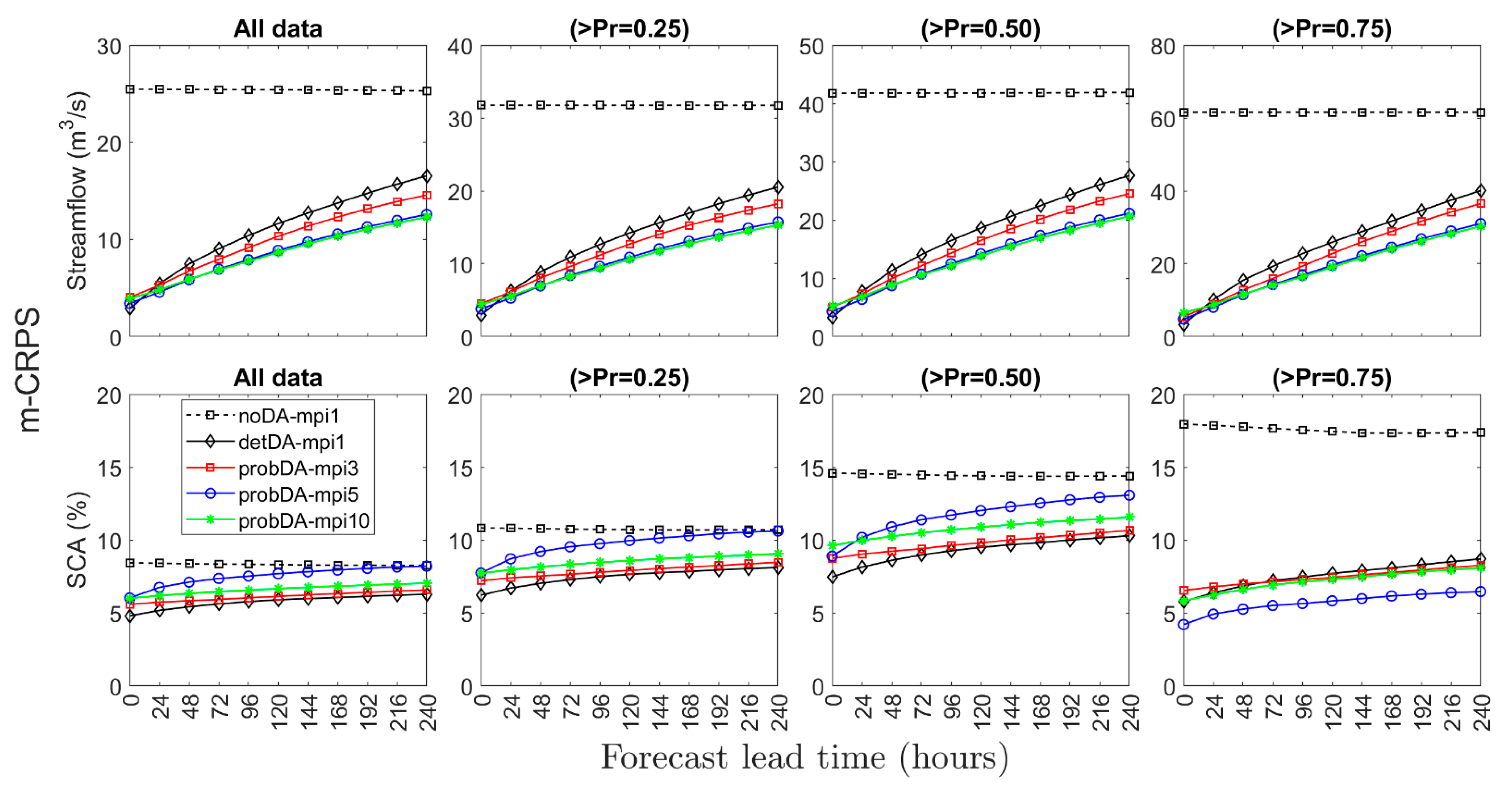
Figure 8 compare the forecast performance using m-CRPS and BSS metrics for VarDA and MP-VarDA experiments, respectively. The performances of the noDA-mpi1 experiment are also shown in the related figures. Since m-CRPS has the same unit as the observations, it provides useful information about the assessment. The m-CRPS of the deterministic experiments are identical to the mean absolute error. The ranges for the streamflow data have wider bounds, and thus the graphs are given in different y-axis scales for m-CRPS, while SCA is kept the same. The m-CRPS of a perfect forecast would be zero, while the BSS for a seamless set of forecasts would be one. Since BSS is always based on a threshold value, the presentations are only available for exceedance probability thresholds, while m-CRPS can be calculated for both all data and forecasts above these thresholds.
The noDA-mpi1 experiment always has the highest error and lowest forecast skill, except for the BSS of the forecasts above Pr = 0.50 in the probDA-10mpi experiment. The data assimilation application seems to improve the performance of hydrological forecasting for both streamflow and snow components. There is a neat order in the data assimilation experiments for the streamflow, which means that m-CRPS values decrease by increasing the number of the model pool in MP-VarDA. According to the snow data graphs, deterministic VarDA gives either less or similar m-CRPS values in comparison to probabilistic MP-VarDA. The order of the error lines is not as representative as in the case of streamflow graphs. Nevertheless, a notable difference can only be stated in the high SCA forecast (>Pr = 0.75), where probDA-mpi5 gives the lowest m-CRPS. On the other hand, BSS skill performance is decreasing over time. The forecast skill of the noDA-mpi1 in streamflow shows that all data have a negative value, indicating the very poor performance of the system without data assimilation implementation. The highest skills are detected for the forecasts above Pr = 0.75 for both streamflow and SCA so that the forecast skills of the high-flows/SCA are better than other forecast groups (>Pr = 0.25 and >Pr = 0.50). The worst skill is detected for the forecasts above Pr = 0.50 in SCA. The lower skills are expected for the forecast above Pr = 0.25.
4. Discussion
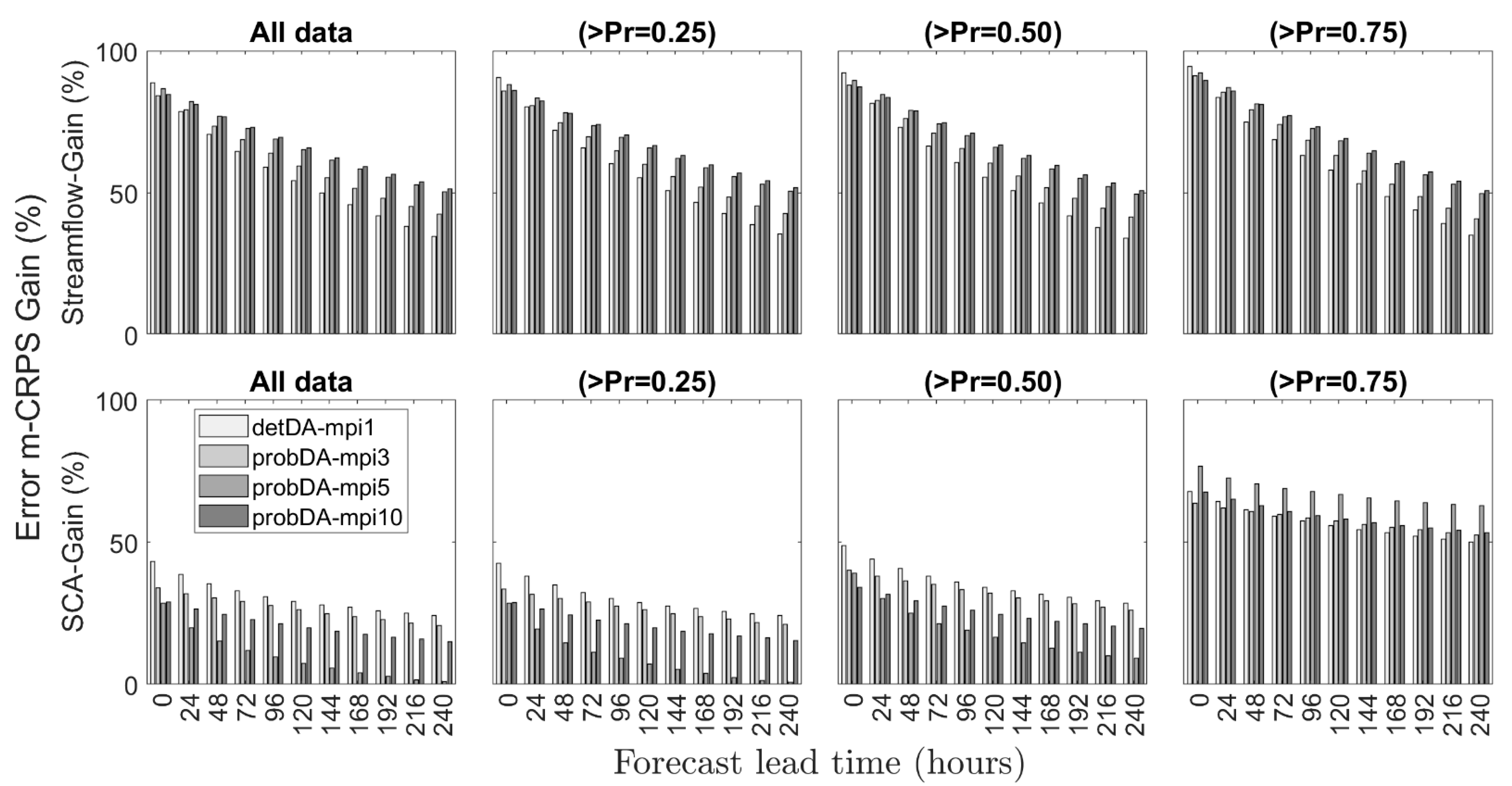
The results are analyzed with percent gains of the data assimilation methods to find the most effective method in the hydrological forecasting system.
Figure 9 compares m-CRPS based error gain (%) for VarDA and MP-VarDA experiments with respect to noDA-mpi1 benchmark simulation. Higher error gains are detected in the MP-VarDA against deterministic VarDA, especially for streamflow forecasts. The error gains intuitively decrease with respect to lead time, but still stay within a considerable level (34% and 50% for detDA-mpi1 and probDA-mpi10 in all data analyses, respectively). Increasing the number of mpi clearly increases the gains. This situation was observed for all data, as well as in different forecast groups above the thresholds. Therefore, it can be stated that MP-VarDA outperforms VarDA for streamflow forecasts in the case of assimilating streamflow and SCA. There is a limit where increasing model pool instances does not contribute further. For example, probDA-mpi5 and probDA-mpi10 seem to give similar results. Compared to streamflow, lower m-CRPS error gains in SCA were detected for both methods. Additionally, VarDA gives a higher gain for all data and the forecasts greater than Pr = 0.25 and Pr = 0.50, while MP-VarDA slightly increases the gains of the forecasts which are greater than Pr = 0.75, especially for probDA-mpi5. This is also detected for longer lead times. However, it is not straightforward to classify which method or mpi gives more accurate results in a general sense.
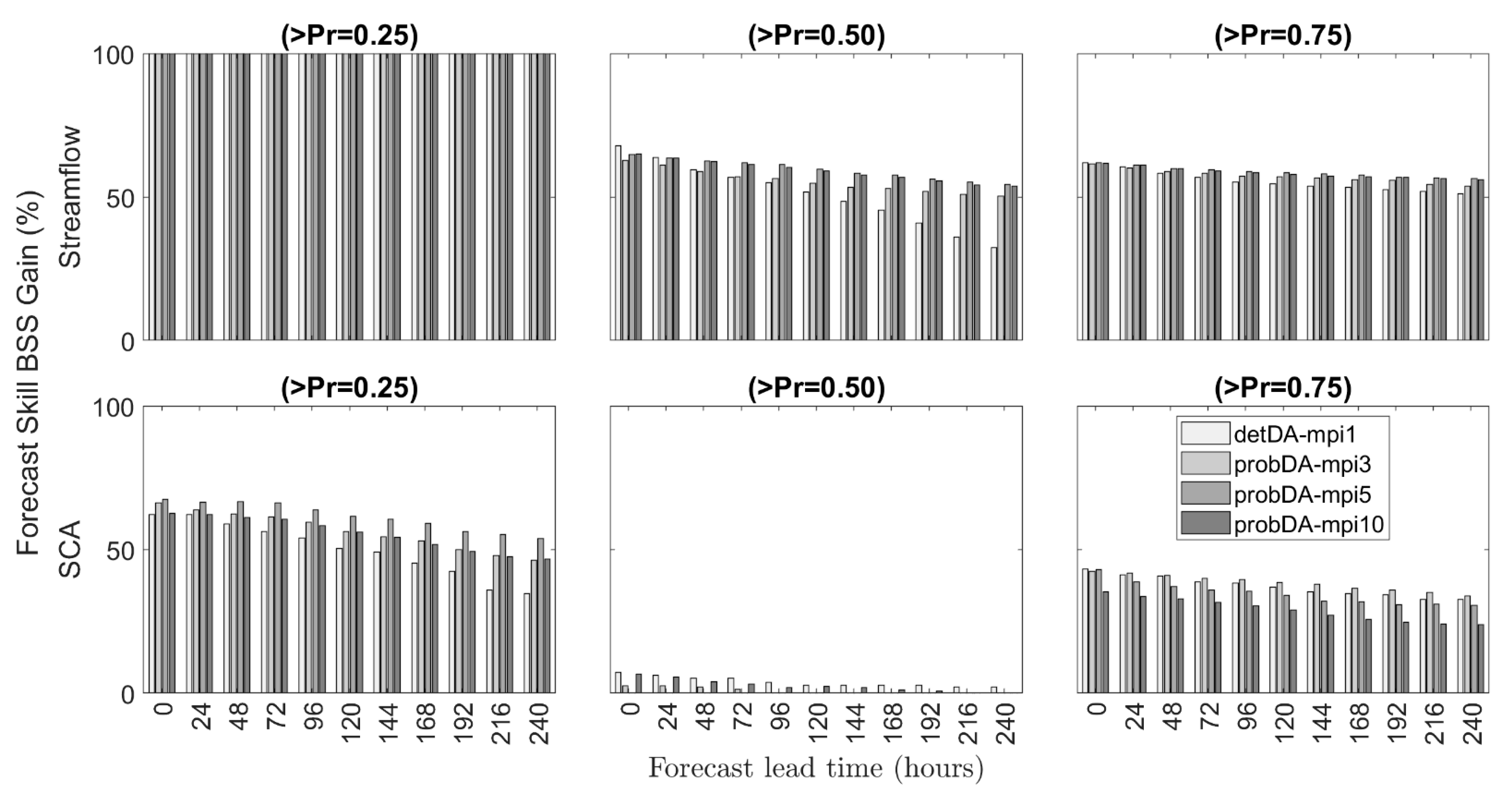
Figure 10 compares the percent forecast BSS-gain of VarDA and MP-VarDA experiments with respect to noDA-mpi1 benchmark simulation. Increasing the mpi in MP-VarDA also enhances forecast skills gains. The gains in streamflow increase above 100% for Pr = 0.25 because of the negative (very poor) BSS performance of the noDA-mpi1 simulation. The BSS gains look similar for the streamflow forecasts above the other thresholds (Pr = 0.50 and Pr = 0.75). The main improvement by MP-VarDA is detected especially for the SCA forecasts above low and high thresholds (Pr = 0.25 and Pr = 0.75). This is also due to the uncertainty capture capacity of the probabilistic case where a larger spread is accounted for in comparison to a single deterministic forecast.
Even though m-CRPS error gains are not increasing as aforementioned, the BSS forecast skill gains seem to be the same or slightly increased in MP-VarDA compared to VarDA. Similarly, the highest BSS gains are detected for the SCA forecasts above Pr = 0.25 following Pr = 0.75. The lowest gain was observed for the SCA forecasts above Pr = 0.50.
As a summary, the mean gain of the whole lead time period (0 to 240 h) was calculated together with their standard deviations for m-CRPS and BSS in
Table 4 and
Table 5, respectively. The mean of the gains for m-CRPS and BSS increase while standard deviations decrease in streamflow from deterministic to probabilistic data assimilation implementation. The highest streamflow m-CRPS mean gain from all experiments within all data and the forecasts above the three thresholds are detected as 67–69% for MP-VarDA, having 5 or 10 mpi. The highest streamflow BSS mean gain of all experiments for all data and within the three thresholds are detected as 63–81% for MP-VarDA, having 5 or 10 mpi. In this study, we kept the variations (F
var) in the Monte Carlo method at 30%, which gives the highest performance according to Alvarado et al. [
29]. The improvements in streamflow forecasts are similar in comparison to their results. The main difference is that the number of mpi is assessed for the first time in this study, and it is found that increasing the number of mpi significantly improves the model performances until a threshold mpi, especially for streamflow metrics. Thus, increasing the model pool seems to converge to a limit where additional gains do not make a significant contribution.
The SCA gains are not appreciated as much as the streamflow, but the models seem to be more robust since they account for the snow component, which is the main driver of the hydrological process. The highest SCA m-CRPS mean gain from all experiments considering all data and the forecasts above the first two thresholds (Pr = 0.25 and Pr = 0.50) are detected as 31–36% from the deterministic VarDA method (1 mpi). However, the maximum SCA m-CRPS gain is calculated as 68% for the forecasts above the upper threshold (Pr = 0.75) in one of the probabilistic experiments (probDA-mpi5). BSS gains of SCA have a different (i.e., not regular) order compared to streamflow. The highest SCA BSS mean gains of all experiments are 12%, 4%, and 47% for probDA-mpi5, VarDA, and probDA-mpi3, respectively. Therefore, the improvement in streamflow seems to decrease SCA performances in MP-VarDA implementation.
Another reason for the variations in SCA performances might be attributed to the assimilation of snow states where SCA is indirectly calculated in the hydrological model. On the other hand, the reduction in AD might affect the performance of SCA in data assimilation application. For example, probDA-mpi5 shows the lowest m-CRPS SCA gain for all thresholds except for Pr = 0.75 (stands for the high SCA values) and this gain is the highest among the others. This could be related to the representation of CFMAX parameter distribution (refer to
Figure 5) of mpi5 among the other model pools and the lower capability of initial state updating of the forecasting during more complex accumulation and melting seasons (refer to
Figure 6 which appears to present lower representation of accumulation or melting seasons with overestimations). We should also keep in mind that CFMAX is a sensitive parameter, which means that a little variation of this parameter could result in large changes especially in SWE, and thus in SCA.
Since a low CFMAX parameter (degree-day factor) causes higher SCA preservation in the model itself (due to slower melting), the overestimation of SCA can result in lower m-CRPS gains in the forecasts above Pr = 0.25 and Pr = 50, but a higher gain for the forecasts above Pr = 0.75 threshold. Additionally, streamflow is dominated by 21 parameters, while only a few of them are directly associated with snow components. This makes the estimation of SWE and indirectly SCA estimation more difficult. On the other hand, BSS gain variation in SCA indicates the complexity of ensemble spread for SCA in the probabilistic method, thus yielding variable best forecast skills. It is also important to keep in mind that SCA still includes uncertainties associated with the temporal and spatial representation of the snow storage.
5. Conclusions
The data assimilation application is a useful technique for a reliable hydrological forecasting system. Integration of data assimilation is especially more challenging in snow-dominated regions due to the complexity of snow processes and limited observations. This study analyzes the forecast performance of multi-parametric probabilistic data assimilation (MP-VarDA) coupled in HBV hydrological model. Streamflow and SCA forecasts up to 10 days are generated using a benchmark simulation without data assimilation application, a deterministic model based on VarDA method, and several probabilistic models based on MP-VarDA method. Since MP-VarDA requires multi-parameterization, Monte Carlo simulation was applied to derive multiple sets of model parameters; however, it is not practical to account for all of them in a real-time forecasting system. In order to make a fair judgment, here we used the same mother model pool to determine both deterministic and probabilistic parameters. To capture model uncertainty without increasing the number of model parameter sets, AD method shows robust representativeness by keeping the maximum amount of parametric uncertainty in the remaining sets. The utilization of AD method in MP-VarDA also enables us to integrate probabilistic methods in the real-time forecasting system more efficiently since probabilistic data assimilation has a higher computational cost relative to deterministic counterpart. The study also reveals the effects of different model instances integrated with a probabilistic assimilation approach. The data assimilation method can incorporate the model pool and improve the hydrological model’s initial states.
In conclusion, we have summarized certain take-home messages and future recommendations below:
The results show the supremacy of MP-VarDA against deterministic VarDA, especially for streamflow forecasts. MP-VarDA reduces the forecast error (m-CRPS) and provides larger forecast skill (BSS) by having probabilistic initial states and ensemble forecasts based on the multi-modeling scheme. The method gives more robust results for different forecast groups above certain threshold values selected from exceedance probabilities. These results should encourage operators to adopt pools with multiple model instances to consider model uncertainty in their forecast estimation.
Considering the data limitation in the upper snow dominated basins, most of the studies in the literature rely on the conceptual semi-distributed approaches. The study was also tested with a single rainfall-runoff relationship through the HBV hydrological model. Our approach takes the advantage of novel assimilation methods and enriching the method with probabilistic states to set up a more reliable forecasting system. The method was also tested in a closed-loop mode which mimics the real-time hydrological forecasting system, and the study demonstrates for forecasters/practitioners that MP-VarDA method can better capture structural uncertainty and improves initial states even using a single hydrological modelling environment.
Assimilating snow with streamflow through hydrological modeling improves both deterministic and probabilistic data assimilation methods. However, considering the complexities of snow accumulation and melting processes, we cannot propose a single best method for SCA forecasts.
We also revealed the impact of selecting different sizes of model pools in a forecast system for a snow-dominated area. Increasing the number of the model pool has a clear impact up to a certain limit on the performance of streamflow forecasts. On the other hand, SCA forecasts are mainly dominated by fewer and more sensitive parameter sets and increments of mpi in MP-VarDA configuration might still increase the forecast performances by capturing better sampling of snow modelling representation.
Future studies should assess and compare these results under numerical weather prediction systems rather than observed meteorological inputs. Even though SCA-SWE is represented by a bilinear depletion function, the more realistic way could be established by a hysteresis. Additionally, in case of having satellite-based SWE, the assimilation can be employed directly by SWE observations so that uncertainties related to the SCA-SWE transition could be reduced.


