Article

Shear-Wave Anisotropy Measurements in the Crust from Receiver Functions: An Interplay of Lower and Upper Crustal Anisotropy

by
Kevin L. McCormack
1,*,
Mark D. Zoback
2,
Andrew W. Frederiksen
3 and
Noam Z. Dvory
1
1
Energy and Geoscience Institute, University of Utah, Salt Lake City, UT 84112, USA
2
Department of Geophysics, Stanford University, Stanford, CA 94305, USA
3
Department of Earth Sciences, University of Manitoba, Winnipeg, MB R3T 2N2, Canada
*
Author to whom correspondence should be addressed.
Geosciences 2023, 13(3), 79; https://doi.org/10.3390/geosciences13030079
Submission received: 7 February 2023 / Revised: 3 March 2023 / Accepted: 7 March 2023 / Published: 10 March 2023

Abstract

:
We report a study using teleseismic P-wave receiver functions to infer the orientation of the maximum horizontal principal stress from the direction of upper crustal shear-wave velocity anisotropy. We apply an inverse approach using the Neighborhood Algorithm to conduct a nonlinear search, attaining a best-fitting crustal model that includes shear velocity anisotropy. Unlike previous methods reported in the literature, this method is able to distinguish anisotropy in the upper, brittle crust from that in the lower, ductile crust in certain instances. We apply this method to teleseismically recorded earthquakes in the Central Valley of California, the Permian Basin, Texas, northern Oklahoma and sites near the San Andreas Fault in California. Of the forty-one stations to which we apply this method, twenty have a good apparent signal. A misfit calculation is performed by calculating a zero-lag cross-correlation coefficient for each modeled receiver function with the data for a given back azimuth range. While the fast polarization direction in the upper crust of some of these stations aligns with independent indicators of the direction of the maximum horizontal principal stress, the fast direction in the upper crust at other stations does not, apparently indicating that the anisotropy was resulting from a different mechanism.

1. Introduction

Knowledge of stress orientation and relative magnitude in the crust are important for geo-energy development and geologic carbon storage. These parameters generally come from four sources of information: wellbore data (principally observations of stress-induced compressional and tensile failures in relatively deep wellbores), earthquake focal plane mechanisms (ideally the inversion of multiple high-quality mechanisms in a given area), relatively recent geologic indicators (volcanic alignments or observations of fault slip) and shear velocity anisotropy from local earthquakes or anthropogenic sources [1]. As originally demonstrated by [2], the application of stringent quality criteria results in remarkable consistency among these methods despite the fact that the depths and volumes of rock sampled vary markedly. Over the past 40 years, there has been considerable improvement in stress determination methodologies as well as the amount of stress data available. Nonetheless, considerable gaps in coverage persist both at local and regional scales in North America and other areas around the world [3,4,5]. In this paper, we present a study investigating whether crustal shear velocity anisotropy determined from receiver functions of teleseismic earthquakes could provide information about stress orientation where no other stress information is available.
Shear-wave velocity anisotropy in the crust could result from two processes—the anisotropy could be related to the current stress state or there could be an intrinsic structural anisotropy due to aligned fractures, fabrics, or foliation. In the former case where the tectonic stresses are controlling the anisotropy, if the upper, brittle portion of the crust contains pre-existing fractures and faults at many orientations, the faults and fractures oriented roughly perpendicular to the direction of the maximum horizontal principal stress (SHmax) will close and/or there could be dilation of faults and fractures oriented parallel to SHmax. Both processes cause the fast polarization direction of the shear-wave anisotropy to align to the direction of SHmax [6,7]. The degree of anisotropy associated with the closure and dilation of faults and fractures is on the order of 2–4% [8,9]. The latter phenomenon that causes shear-wave anisotropy is the structural alignment of rock fabrics, which is typically greater in the lower crust where ductile flow can align minerals [10]. The degree of anisotropy associated with structural alignment can be as high as ~20% [11]. Due to the difference in the magnitudes of anisotropy from the two phenomena, we expect that if the contribution from fabric-induced anisotropy in the upper crust is slight, then it should be possible to determine the direction of SHmax from the fast polarization direction. On the other hand, if there is significant structurally controlled anisotropy, especially in the lower crust where the effect is amplified by the ductility, we show that the ability to determine the direction of SHmax can be complicated.
We test the inversion to perform a nonlinear search of parameter space to minimize the misfit between synthetic data and the recorded receiver function data of forty-one stations. The remainder of this paper details the methodology of this approach and then analyzes the results to examine the interplay between lower and upper crustal anisotropy and the potential for measuring SHmax in such a manner.

2. Materials and Methods

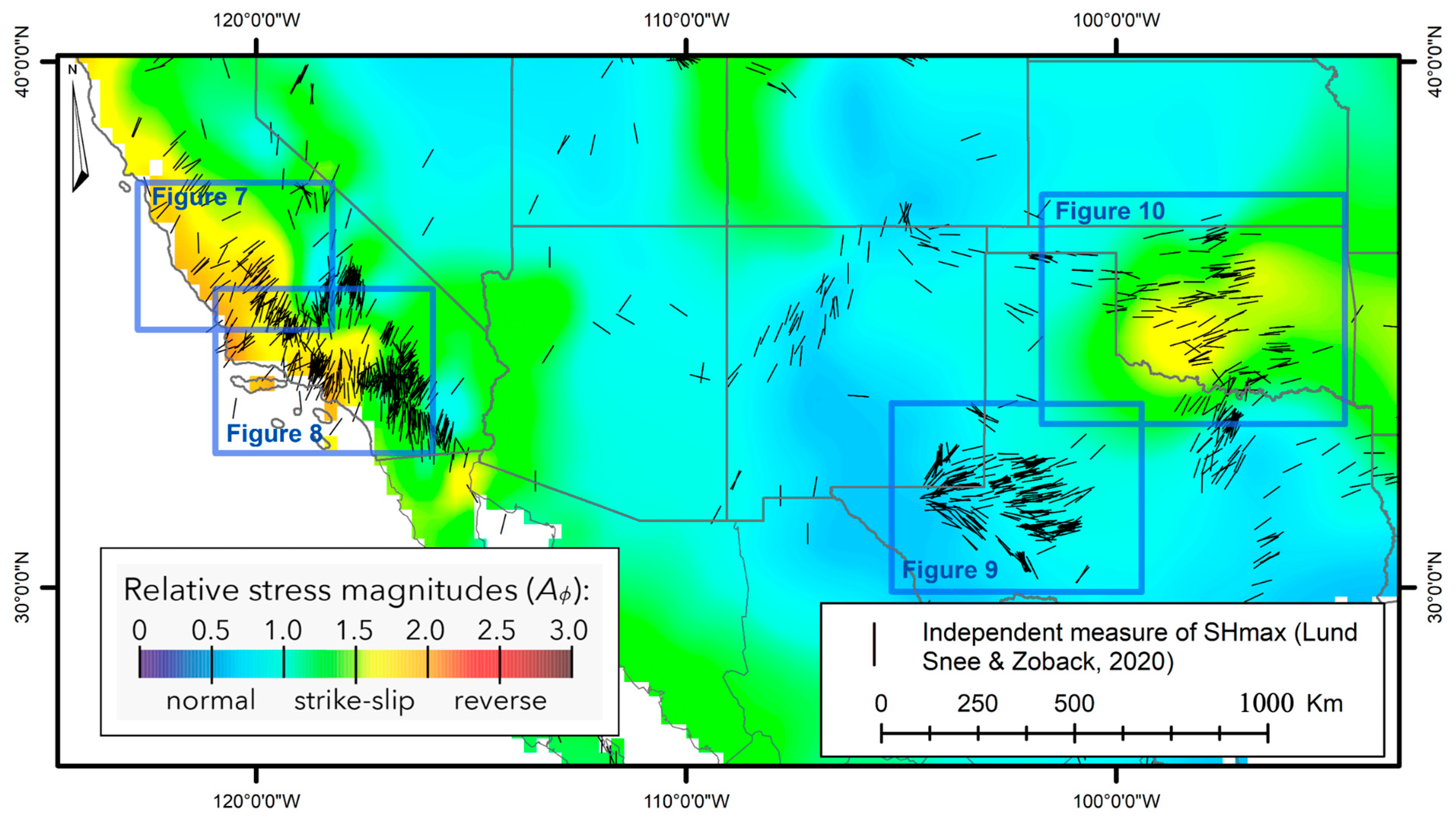
Forty-one stations were analyzed using the Neighborhood Algorithm inversion [12,13]: four in the Central Valley of California, four in southern California, seventeen in the Permian Basin, fifteen in Oklahoma and Kansas, and also the Parkfield station overlying the San Andreas Fault in central California (Figure 1). The southern California stations were chosen because local earthquake shear-wave splitting measurements were performed at nearby stations [14,15]. There are also independent indicators of the orientation of the maximum horizontal principal stress in southern California. The Central Valley and Oklahoma stations were chosen because they had relatively little sedimentary cover, and there are independent stress indicators available [14,16]. The Permian Basin Stations were chosen due to the economic significance of the region. In addition, the number of stations that we analyzed in each region was dictated largely by the computational costs of the inversions. These computational costs are related to the high quantity (>10,000) of receiver functions that were calculated with the total variation deconvolution (Appendix A). The disparity in the number of stations from the California regions to the stable intraplate regions is because we anticipated fewer tectonic impacts on the anisotropy in the latter regions, and thus tested more thoroughly.
The method that we used to assess the anisotropy of the crust using receiver functions is a nonlinear inversion to find a best-fitting model corresponding to the recorded receiver function data. This method has three distinct advantages over shear-wave splitting of Moho converted Ps phases, which is also found in the literature [10,17,18]. First, there is no need to subjectively isolate Ps phases, which despite quality controls, may introduce error into the shear-wave splitting method. Second, events without clear Ps phases can be used, which may contain valuable information about other time periods of the receiver function but may also complicate the stacking. The third advantage of this method is that it could in principle isolate the anisotropy to just the brittle, upper crust where the stress can be controlling the anisotropy.
The method we employed was developed originally by [19] and furthered by [20,
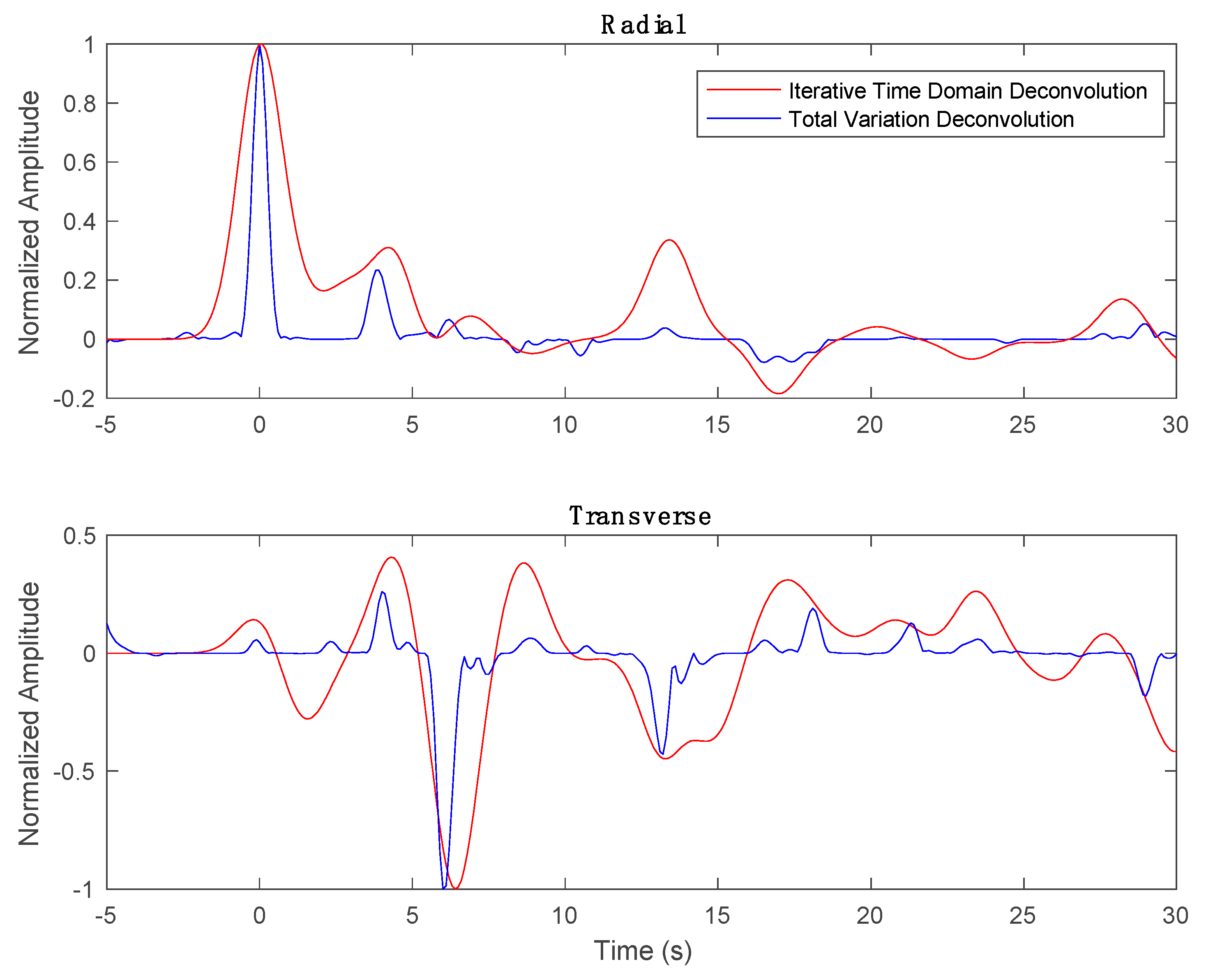
21]. The first step in the methodology was to deconvolve the seismograms using the total variation method outlined in Appendix A. The azimuthal direction from which an earthquake arrives at the station (back azimuth) is important in the treatment of anisotropy because patterns in the amplitudes and arrival times of waveforms with different back azimuths can be used to calculate the velocity anisotropy beneath the station. Thus, we binned the receiver functions into 20-degree back azimuth bins and stacked the receiver functions within each bin after first correcting for the angle of incidence. The 20-degree bin is subjective and dependent upon the number of events per station. If the bin is too small, there are not enough events to stack. If it is too large, the sensitivity to back azimuth and thus anisotropy is lessened.
Once the raw data were processed for each station, the Ps phase was isolated, and all of the analyses presented below corresponded to inverting for just a narrow window of 2 s before and 2 s after the theoretical Ps arrival, which was acquired from the Earthscope Automated Receiver Survey for each location. The 2 s window was intended to capture the full Ps phase, which was anticipated to be most sensitive to crustal anisotropy. Next, the Neighborhood Algorithm was performed in order to find a best-fitting model for this nonlinear inversion [12,13]. The idea behind the Neighborhood Algorithm is that a set of forward models are calculated from an initial batch of models with randomly selected parameters. Next, a misfit calculation was performed for those initial forward models, and a Voronoi cell was placed around each model in parameter space such that when the next step was applied—a random walk from each of the initial models—the new models fell within the Voronoi cell. The misfit calculation was performed on all the new models. Then, the x number of models with the best misfits performed a random walk within their new Voronoi cells to create the next iteration of models. The parameter x was chosen by the user and was a function of both the desired completeness of search of the parameter space and the number of free parameters. The process iterated until convergence, which given the complexity of our model took about 40,000 models and 500 iterations for each station.
The forward modeling was performed using the software RaySum [22], which uses a ray theoretical algorithm to calculate synthetic seismograms for various back azimuths, dipping layers, and anisotropy. The most computationally expensive part of the inversion was performing the total variation deconvolution on the many thousands of seismograms generated by RaySum (Appendix A). The misfit calculation was performed by calculating a zero-lag cross-correlation coefficient between each modeled receiver function and the data with the corresponding back azimuth range within the four second Ps window. We used this coefficient averaged over every back azimuth bin to assess the goodness of fit, but because the Neighborhood Algorithm minimizes misfits, we had to subtract that value from one in the inversion.
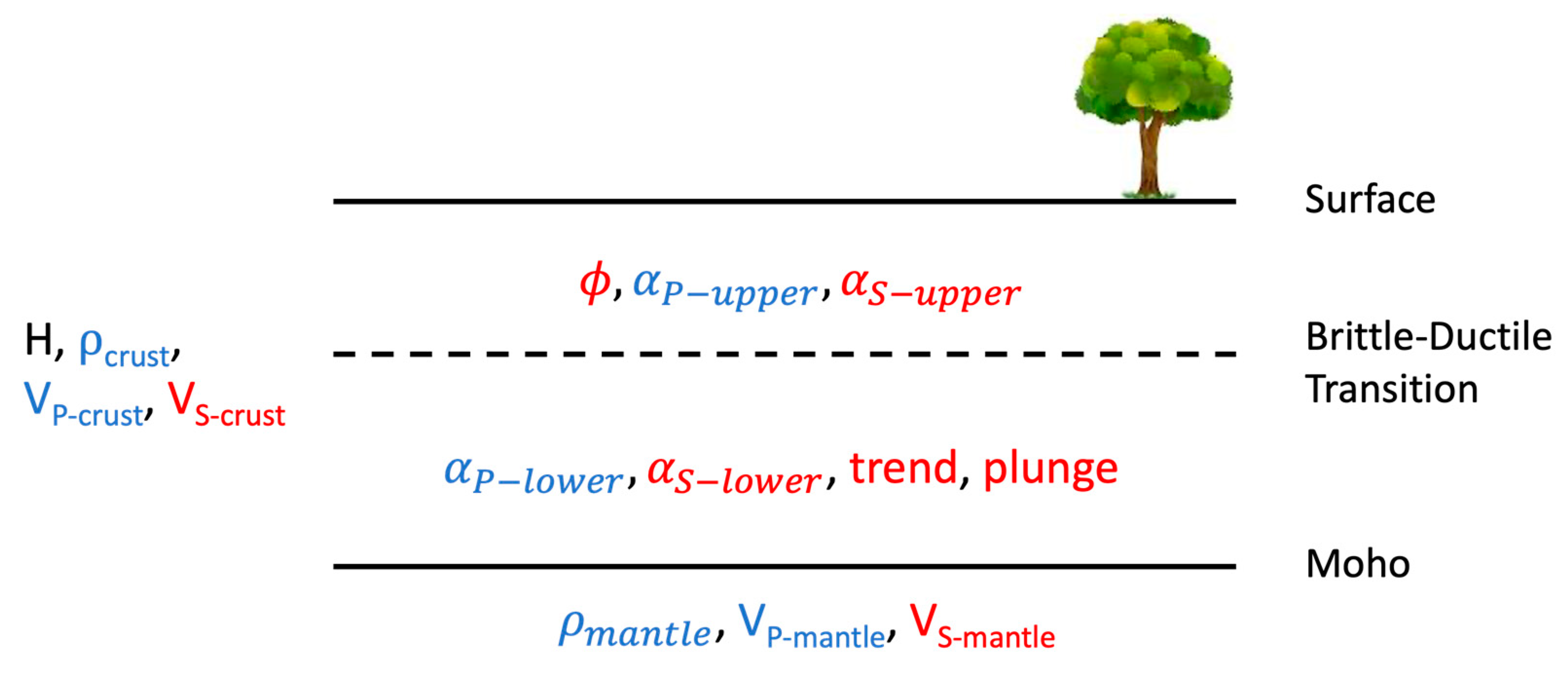
The model we used for the forward calculations has three layers: the mantle, the lower crust, and the upper crust (Figure 2). The motivation for separating the crust into the lower and the upper is that the stress-controlled anisotropy is the result of the closure and dilation of fractures, which would only occur in the upper, brittle portion of the crust. For our objectives it was necessary to split the crust in this fashion. We inverted for a model with only seven parameters (Table 1) by prescribing values for the thicknesses of the upper and lower crust obtained from the Earthscope Automated Receiver Survey H-k stacking [23]. We used a fixed relation between the P- and S-wave anisotropy ( 1.64   A n i P = A n i S ) and an empirical formula for the density of each of the free layers ( ρ = 1.6612 V P 0.4721 V P 2 + 0.0671 V P 3 0.0043 V P 4 + 0.000106 V P 5 ) [24], and by assuming the V P = 3 V S 1.73 V S , which is the case for a Poisson solid. For a detailed argument on why fixing the P-wave anisotropy to the S-wave anisotropy is valid, see Appendix B. In this design, we assumed averaged mechanical properties for the entire crust, and the brittle/ductile transition mattered only for the anisotropy. Although eighteen parameters were used in the forward modeling, only the fast polarization direction of the upper crust (ϕ), the anisotropy percentage of the S-waves of each of the lower and upper crust (αs), the trend and plunge of the anisotropy of the lower crust, and the shear velocity of the averaged crust and uppermost mantle (Vs) were inverted for, because the other parameters were either calculated from those seven or obtained from a reference. The Neighborhood Algorithm only searches over user-prescribed ranges of values for each free parameter. Those ranges are given in Table 1. The output of each inversion is tens of thousands of models with corresponding misfits. These were ordered by ascending misfit and the lowest-misfit model was assessed for the brittle fast polarization direction.

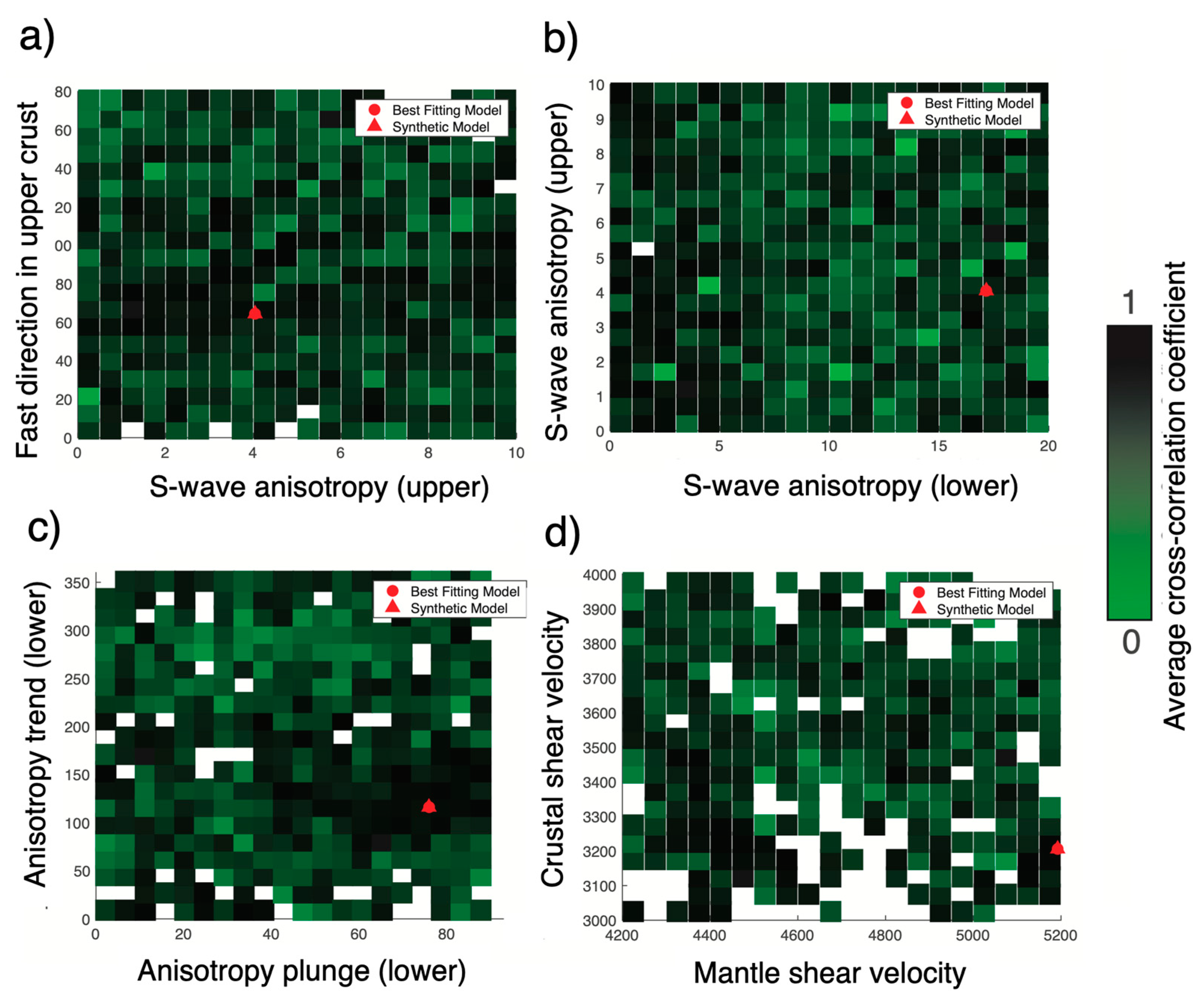
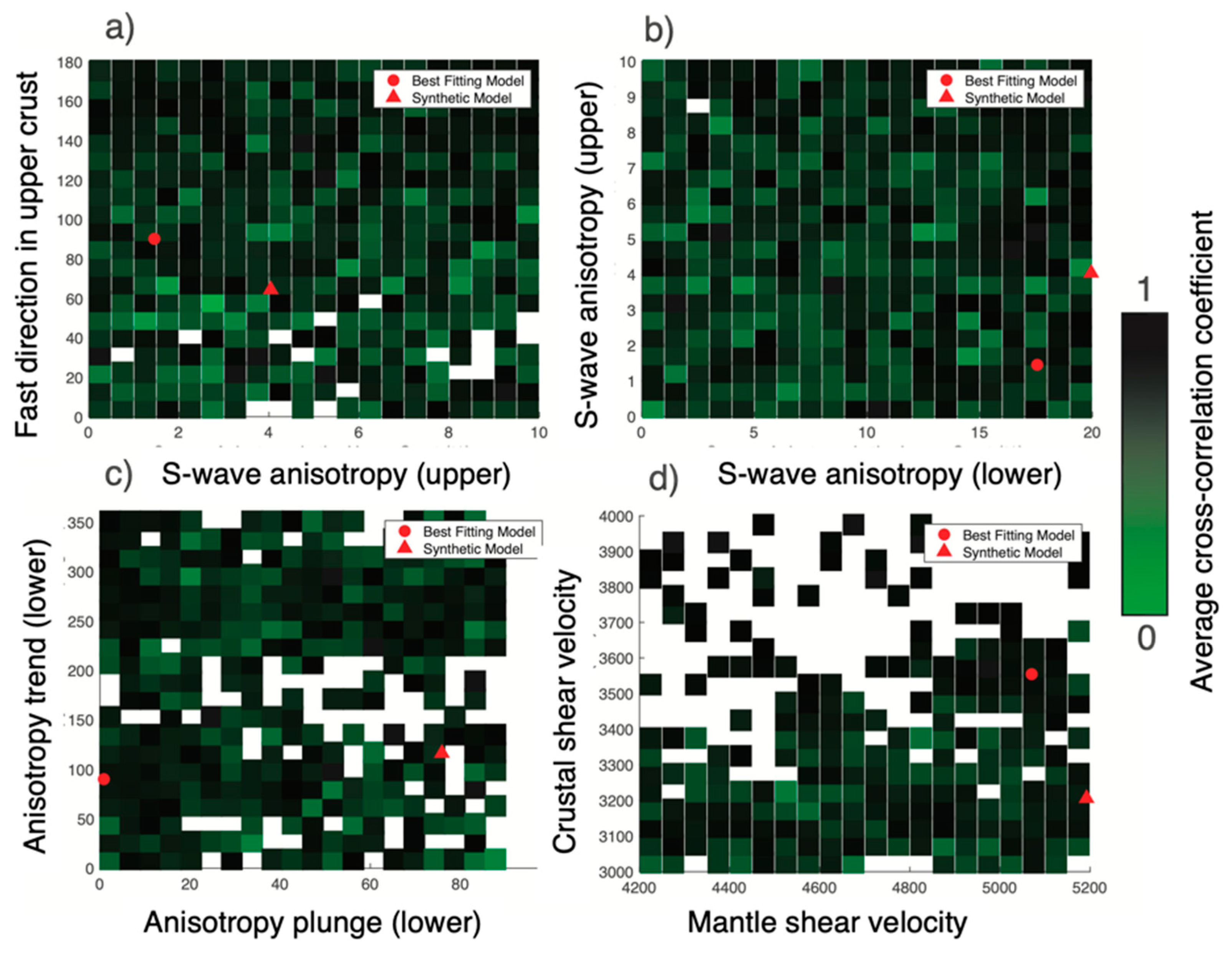
Testing the Inverse Algorithm

We tested the inverse algorithm using the deconvolution scheme for the receiver functions described in Appendix A against data from a synthetic model. For the purposes of the synthetic test, we used a model with anisotropy in both the upper and the lower crust, such that the successful results lend credence to the ability to differentiate between anisotropy in the two layers. The inputs and inverted parameters are shown in Table 2. We chose to plot the model parameters in pairs of similar physical significance (e.g., Vs crustal and Vs mantle), color-coded by the lowest-misfit model in each region of parameter space (Figure 3). These plots allow for the quick assessment of where in the user-prescribed parameter space the best models reside. That is, in the dark squares in Figure 3, the misfit is low and there are good models. In the bright green squares, the misfit is high, and the Neighborhood Algorithm will avoid these regions. The four plots corresponding to the seven parameters can be seen in
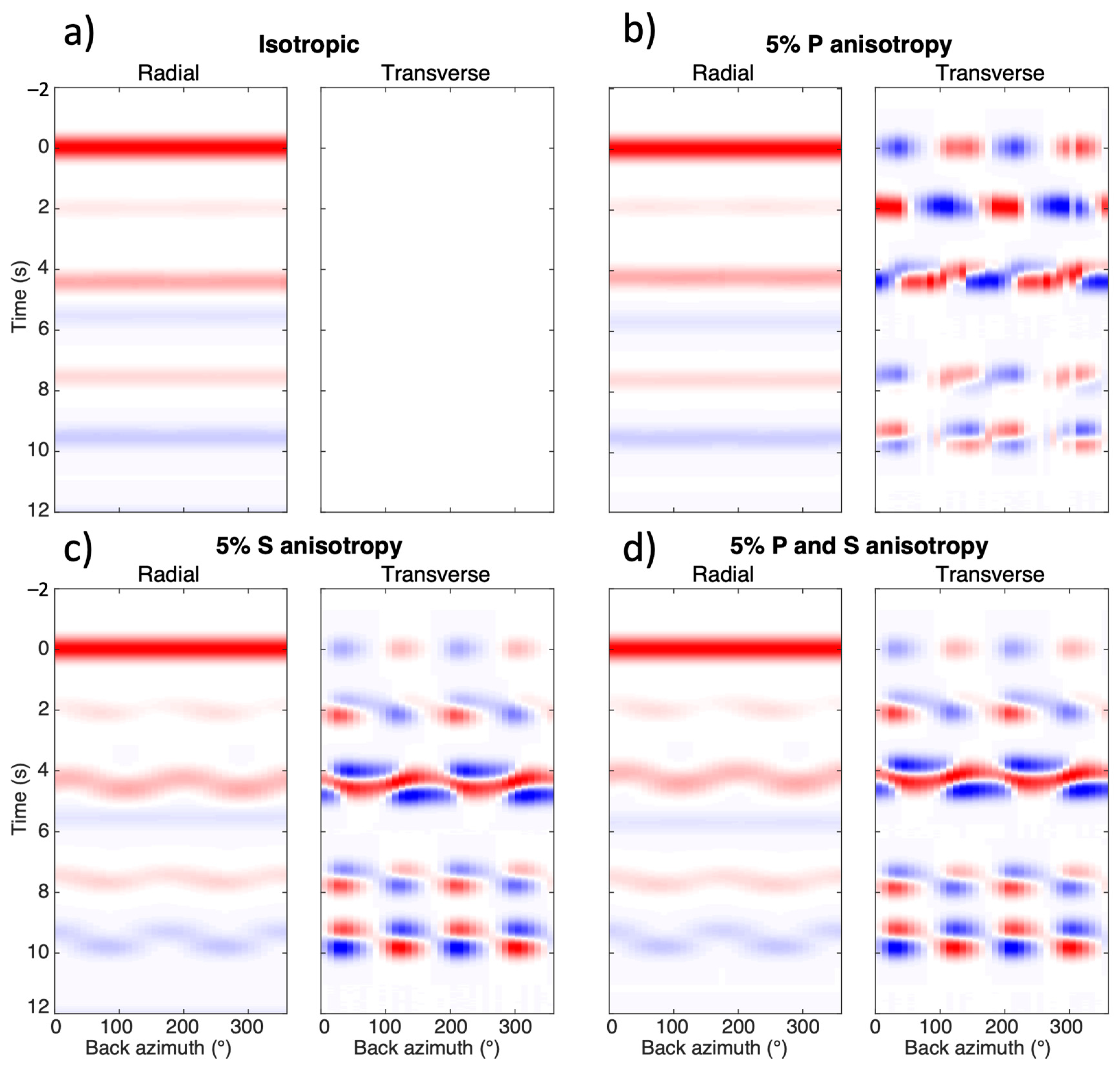
 Figure 3 (the % S-wave anisotropy is plotted twice for visualization purposes—there are an odd number of parameters). The inversion captures all the parameters, and the waveforms were recovered effectively (Figure 4). In nearly every parameter, an almost perfect fit was observed between the best-fitting model and the known input. Thus, for this test, the inversions performed effectively.

3. Results

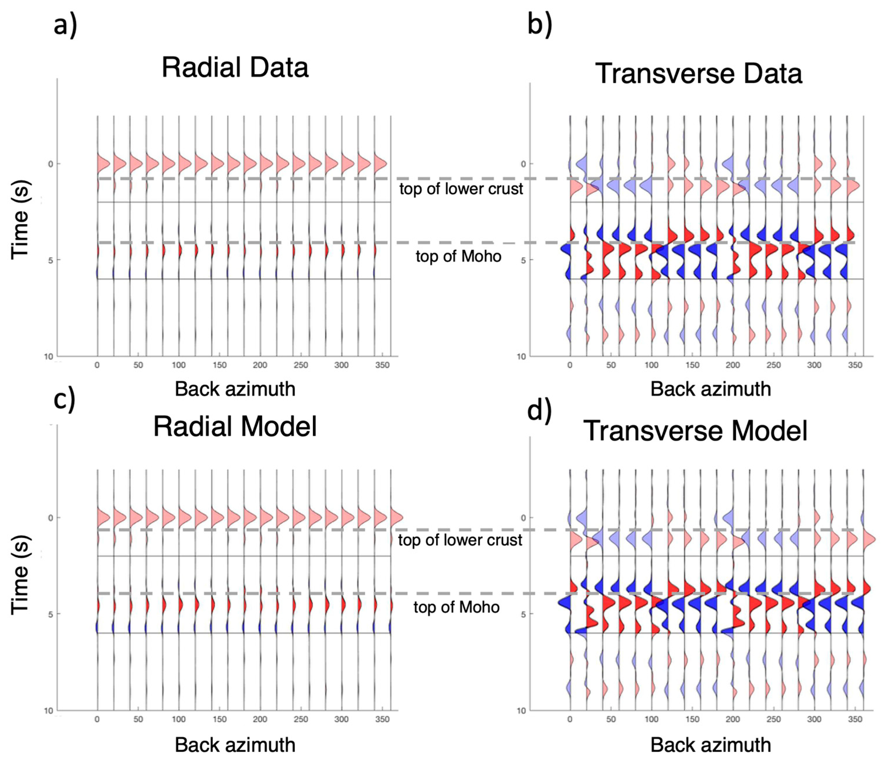
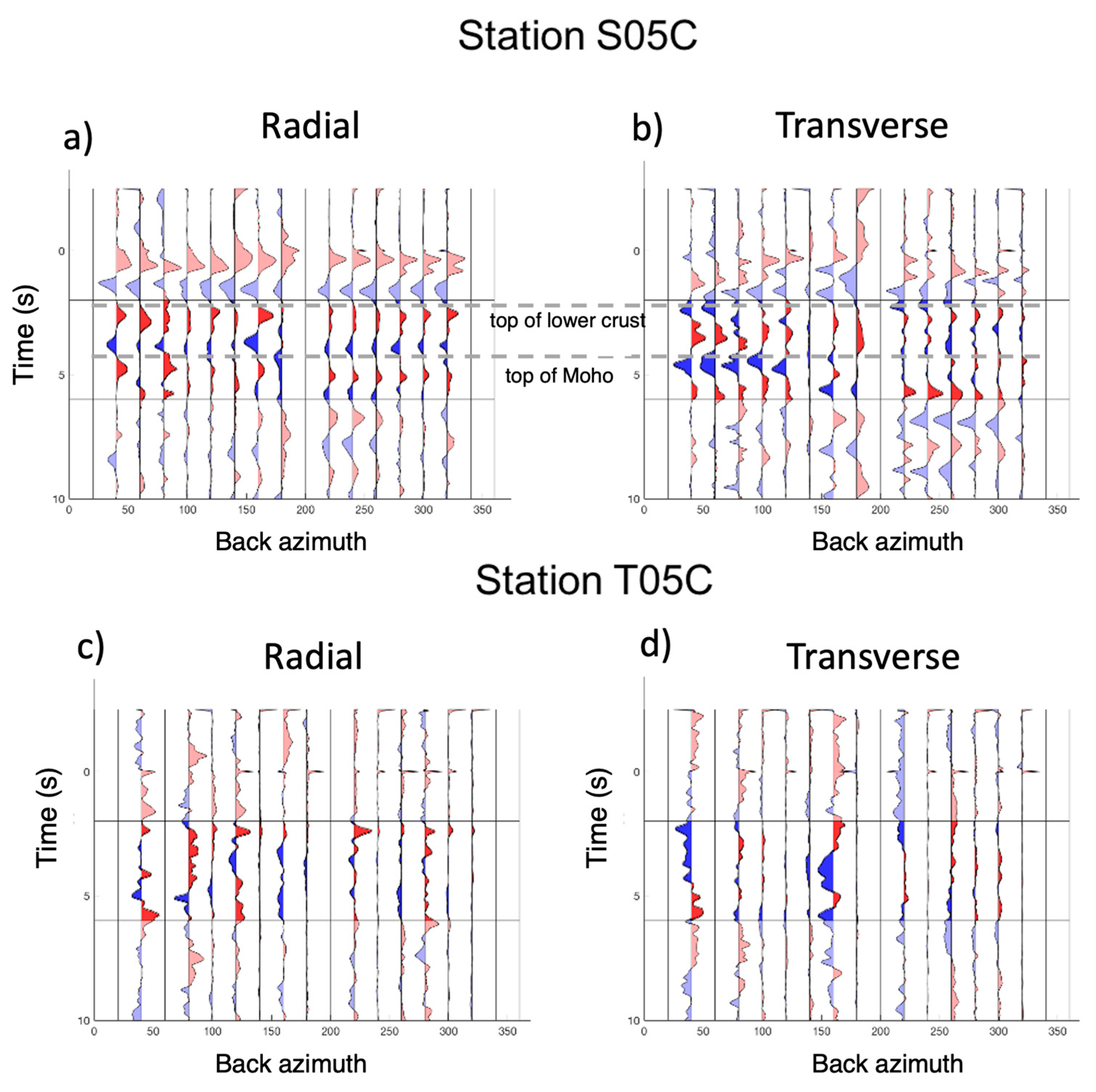
It is instructive to assess the signal quality of the processed data. There is often poor signal-to-noise ratio in the data, so the results for most of these stations could not be used (Table 3). Therefore, we both qualitatively assessed the signal-to-noise ratio of the stacked data (Figure 5), differentiated by back-azimuth, for each station, and measured the average zero-lag cross-correlation coefficient for each of the best-fitting models relative to the data. The qualitative assessment of signal-to-noise ratio was quality control, in which we checked for the presence of distinct P and Ps phases in the receiver functions. We discarded any results where there were not distinct P and Ps phases or there was an average cross-correlation coefficient value below 0.30.
The average zero-lag cross-correlation coefficients of Table 3 are an indication of the quality of the inversion, yet it is helpful as well to visualize the results. 
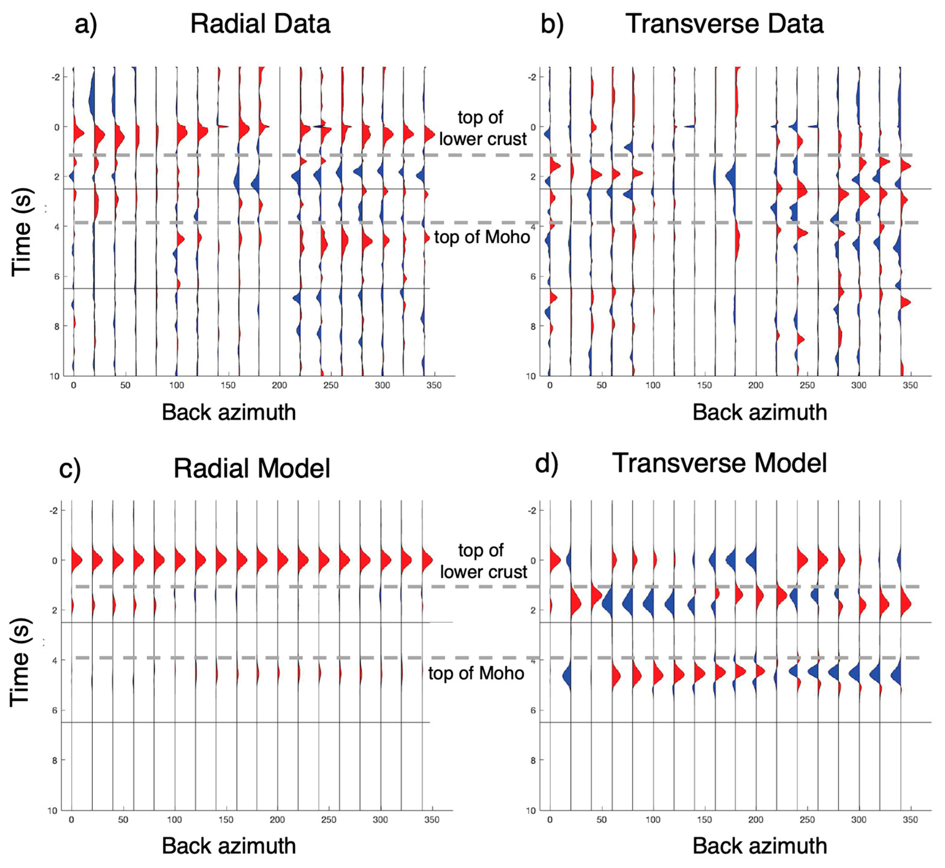
Figure 6 shows the raw data as well as the waveforms from the best-fitting model for the PLM station in southern California. According to the cross-correlation coefficient, this is the highest quality of all of the twenty inversions, although station W32A in Oklahoma has nearly the same cross-correlation coefficient. Visual inspection also corroborates that the inversion was successful. While the waveforms from the data are not captured perfectly, the match is sufficient to validate the efficacy of our methodology. Table 4 shows the parameters of the best-fitting model for all twenty stations tested.
The results detail a comparison of the direction of the maximum horizontal principal stress, as understood from previous studies, to the fast polarization directions obtained from our inversions. The previous studies on maximum horizontal principal stress directions rely on several methods. First, there are earthquake focal plane mechanism inversions, which take regional data on the radiation patterns from earthquakes to invert for the state of stress that best describes the data [3]. Second, wellbore data, whether drilling-induced tensile fractures or wellbore breakouts, are used to provide this measurement [3]. Third, the alignment of hydraulic fractures, typically determined from microseismicity, is used [3]. Finally, shear-wave splitting measurements from local earthquakes constrain the direction of crustal anisotropy [14,15]. These measurements from previous studies are referred to here as independent measurements of SHmax.
We hypothesize that there are four separate phenomena represented by the fast polarization directions of our inversion. First, the stresses are acting on quasi-randomly oriented fractures and faults, inducing a stress-controlled shear-wave velocity anisotropy. Second, there are some stations that lie close to large, crustal-scale discontinuities such as the San Andreas or Elsinore faults, and as was shown in [9], these features tend to align the shear-wave velocity anisotropy to the strike of the discontinuity. Third, the dip of the Moho can often cause effects on receiver functions that are nearly indistinguishable from anisotropy [25]. Finally, the inversion has been observed to be less accurate at high values of lower crustal anisotropy (Appendix C). Therefore, we see the combination of the first three factors in each of the fast polarization directions, and we see the fourth factor in the subset of the polarization directions that have high lower crustal anisotropy.
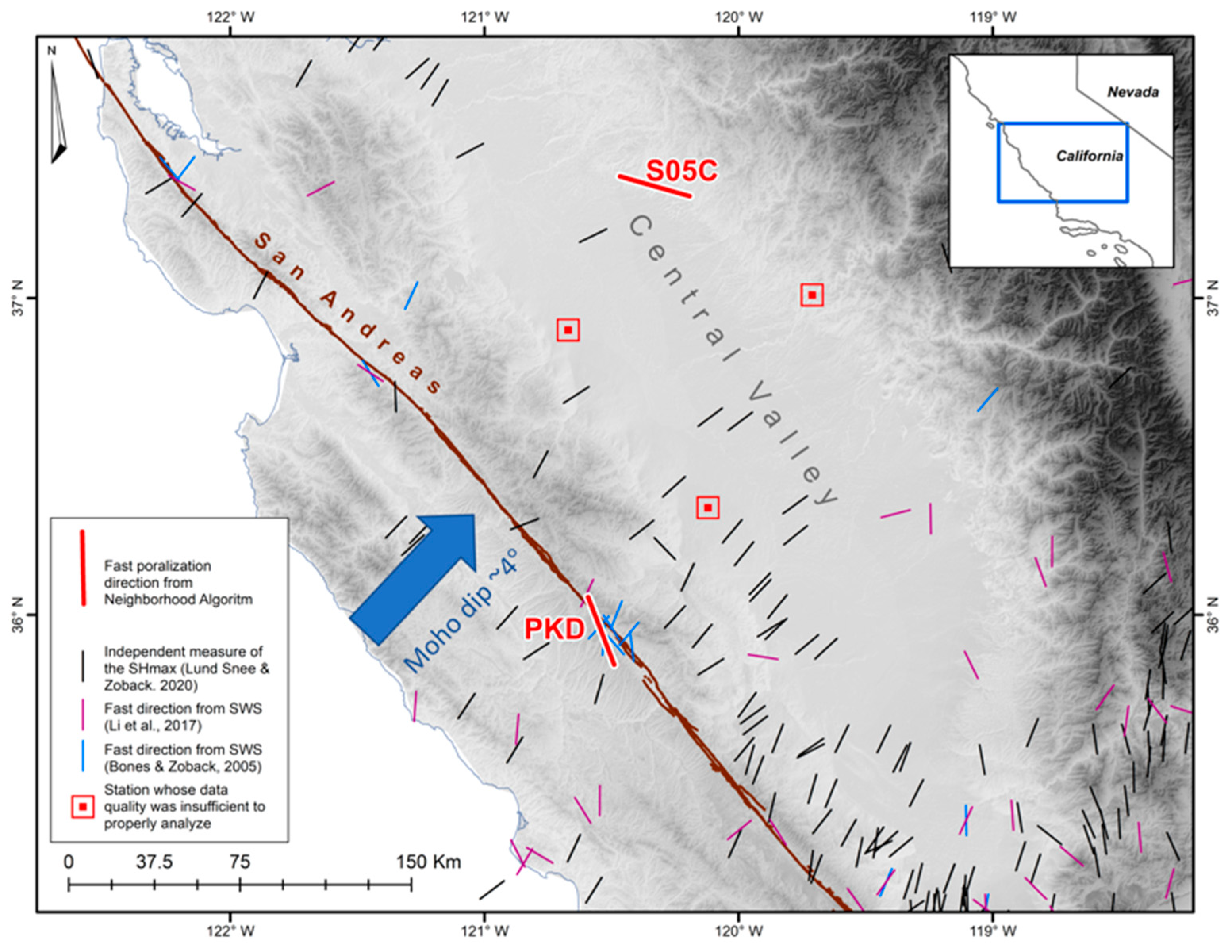
In Figure 7, we see the effect of the data quality wherein only two out of the five stations were able to be analyzed. Indeed, the S05C fast polarization direction aligns poorly with the independent measurement of SHmas, as noted by [3]. In contrast, the data from the PKD station along the San Andreas fault do not align to the known independent stress indicators, which means that that anisotropy is not stress controlled. The PKD inversion result does align with the strike of the San Andreas Fault, however, which may mean that the inversion has identified structural anisotropy. The blue arrow indicates an interpretation of the dip of the Moho [26]. The reason for the small number of stations tested (five) is due to the computational cost of these inversions, and we decided to use the majority of our resources in Texas and Oklahoma where there is not expected to be strong structural anisotropy.
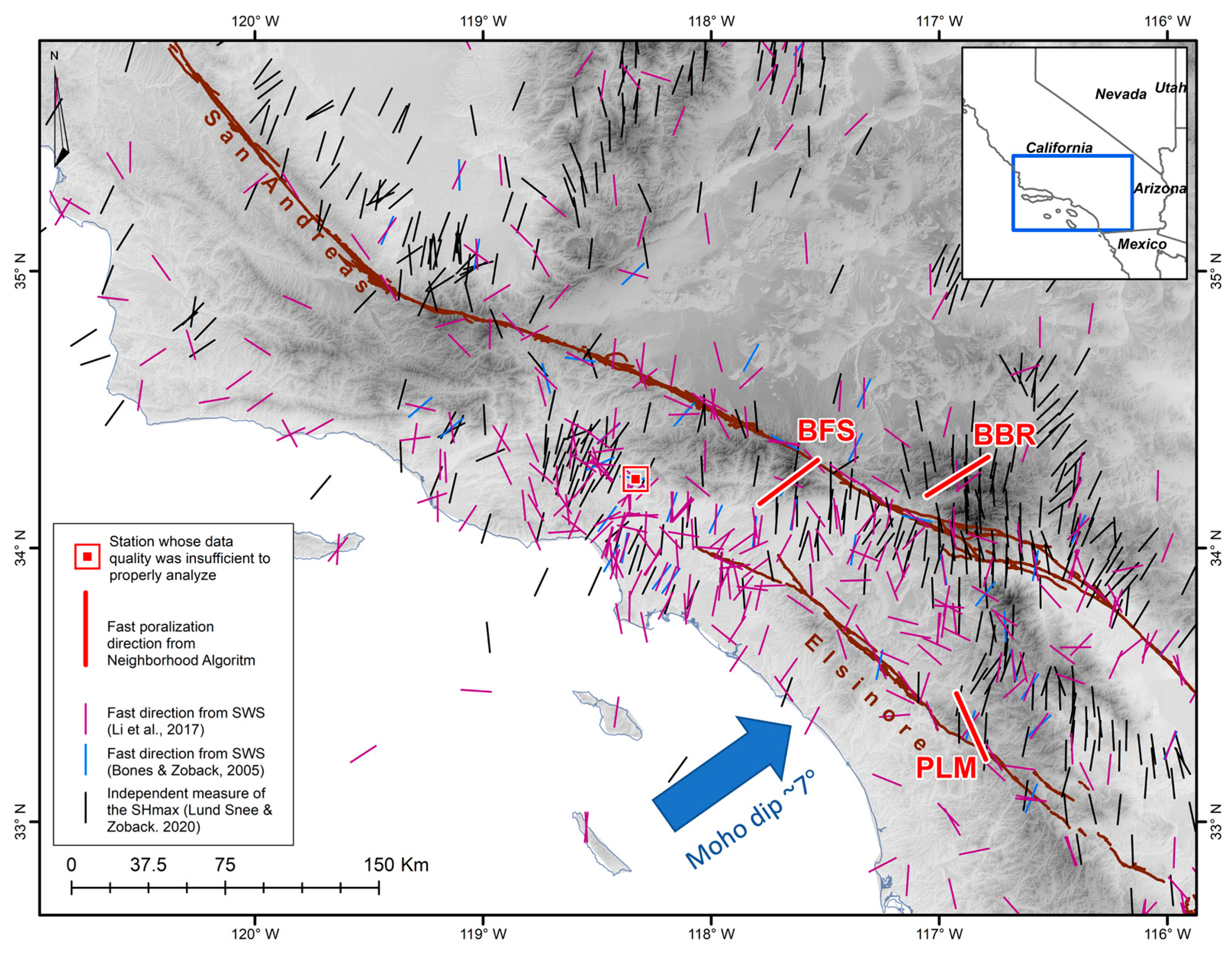
In Figure 8, there are three fast polarization directions that disagree not only with the regional independent measurements of SHmax but also indicators of the regional upper crustal anisotropy [14,15]. This means that the inversion is not obtaining the upper crustal anisotropy for this region, which could be the result of the other three factors influencing the inversion: structural anisotropy, Moho dip, and the limitations of the inversion at high degrees of lower crustal anisotropy. The blue arrow indicates an interpretation of the Moho dip from [27,28], and there is a correlation between that direction of dip and the anisotropy indicators of stations BFS and BBR. The PLM station overlies the Elsinore Fault and aligns well to the strike, which could be an indication of structural anisotropy. Once again, computational cost was the primary impediment to analyzing more stations.
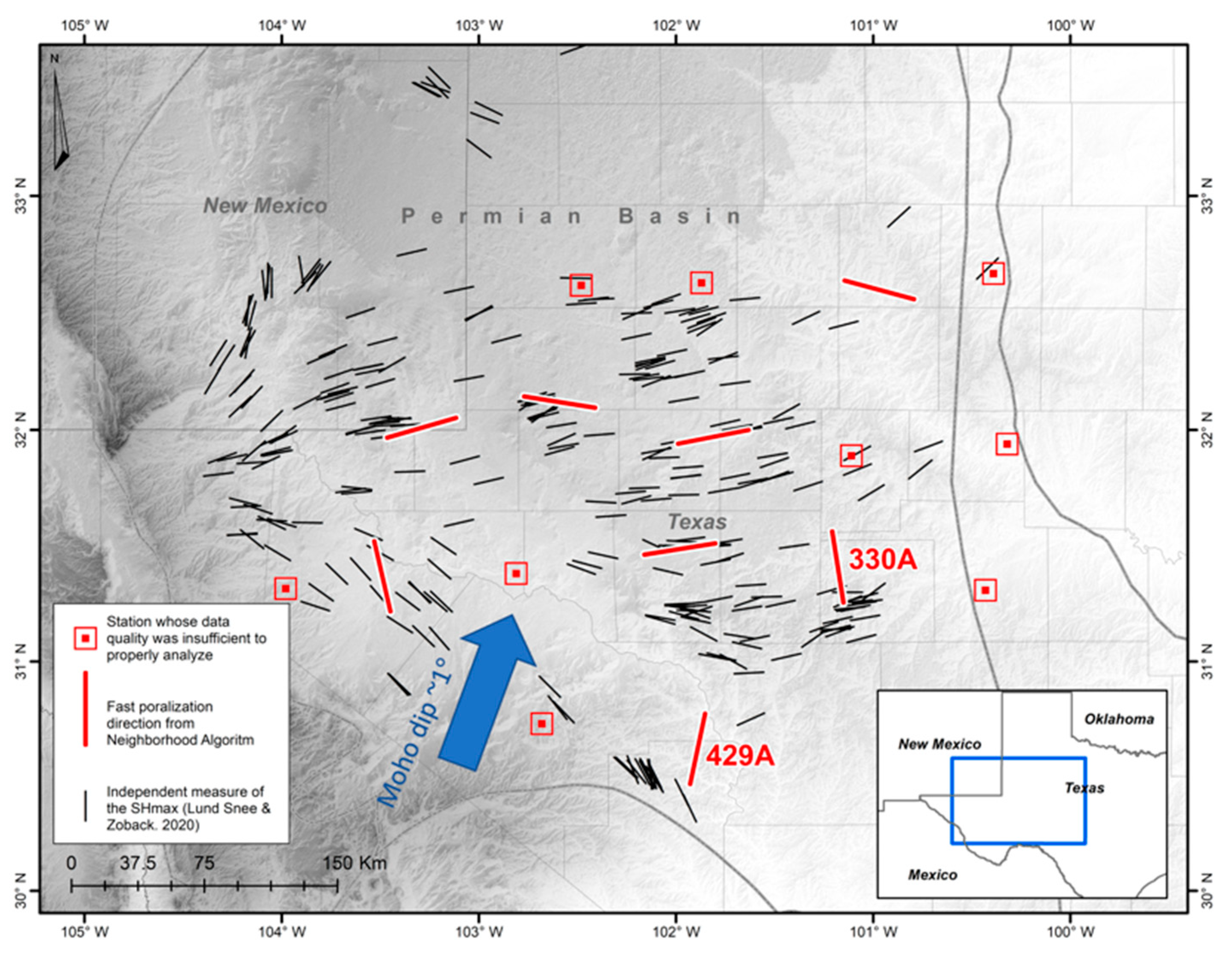
In Figure 9, there are eight out of seventeen stations that had both a qualitatively significant signal-to-noise ratio, and an average zero-lag cross-correlation coefficient greater than 0.30. The average of those coefficients is 0.56. Five of the seven fast polarization directions agree well with the known stress field. The other two (330A and 429A) seem to align at least partially with the Moho dip, and furthermore have lower crustal anisotropy values greater than 18% (see Table 4 for the full best-fitting model results). This mixture of Moho dip, high lower crustal anisotropy, and stress alignment may indicate that in certain subregions the effects from the upper crustal anisotropy might be more pronounced and lead to the good agreement with the stress field, while in other subregions the other three factors are dominant. The Moho dip is interpreted for the Permian basin from Shen and Ritzwoller (2016) [29].
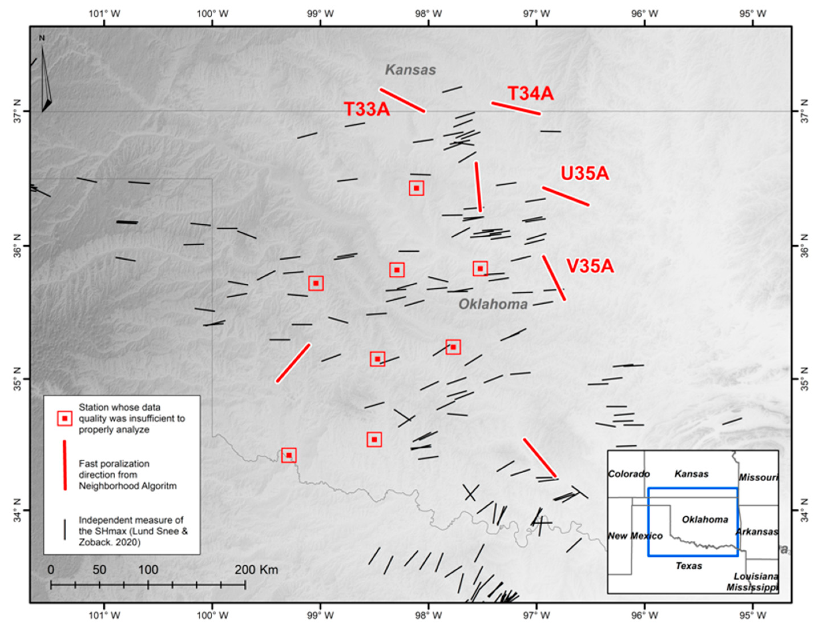
Figure 10 shows some of the complexities of using teleseismic waves to determine the upper crustal stress orientation. Of the fifteen stations analyzed here, seven have sufficient signal. On average, the average zero-lag cross-correlation coefficient is 0.72, which is considerably higher than that of the Permian basin, most likely due to reverberations in the Permian basin sedimentary layers decreasing the signal-to-noise ratio of the receiver functions. Three of the stations in the northern portion of the study region (T33A, T34A, and U35A) exhibit a fast polarization direction that is relatively close to the independent measurements of SHmax. The degree of lower crustal anisotropy according to the best-fitting model for the V35A station is significant (>19%), but the rest of the stations do not have extreme values for the lower crustal anisotropy. We posit that either complicated structural anisotropy due to faulting in the region or fabrics in the lower crust that have been uplifted into the upper crust are the most likely explanations for the moderate performance of the inversion. The Moho dip is not strong or systematic in this region and has thus been omitted from the map [29].

4. Discussion

Refs. [19,21] successfully apply techniques similar to the nonlinear inversion method of this paper to regions in the Tibetan Plateau and Parkfield, California, respectively. In both studies, the authors were interested in anisotropy of the lower crust. Indeed, the potential degree of anisotropy due to mineral alignment may be as high as 20% [11], which is significantly greater than the 2–4% reported for stress-controlled anisotropy in the upper crust [8,9]. Therefore, the upper crustal signature that we want to discern is smaller than the lower crustal and mantle anisotropy wherein there is a greater potential for mineral alignment due to ductile flow. Even though the nonlinear inversion allows us to search for just the brittle crustal anisotropy, the significant contribution from the lower crust still had the potential to obfuscate the results (Appendix C). This is evidenced in our results by the fact that our measurement at the BFS station (Figure 8) did not align to the anisotropy of [14,15]. From this result, it seems clear that the inversion only sometimes successfully differentiated anisotropy between the upper and the lower crust. The other factor that appears to play a role in the results from the nonlinear inversion is the direction and magnitude of the Moho dip. In Southern California (Figure 8), the BFS and BBR stations both seem to align to a steeply dipping Moho, while in the Central Valley (Figure 7) there is no alignment to the Moho dip at roughly 3°. In the Permian Basin, where the dip magnitude is only roughly 1.5°, there are only potentially two stations influenced by the Moho dip (330A and 429A). We must emphasize, however, that the Moho dip depicted in Figure 7, Figure 8 and Figure 9 is only an interpretation of published data, and the true nature of the dip is likely more complicated.
Even in regions where the interplay of lower crustal anisotropy may be too significant to deduce a reliable upper crustal signal, as is seen in many of the measurements of this study, there is still information about the crust contained in these inversions. The measurements that do not align to the direction of the maximum horizontal principal stress may indicate that the structure of the crust is complicated and may be modeled with more sophisticated methods that rely on plunging-axis anisotropy [30]. The results that differ may also represent locations where fabric from the lower crust has been uplifted into the upper crust. The validity of the results that align to the direction of the maximum horizontal principal stress is enhanced by those results that indicate a more complicated structure, in that both reveal different, yet interrelated, properties of the crust. A challenge of this technique is that it may not be possible to discern between complicated structure and stress without prior knowledge of the stress state or crustal structure.
One of the potential problems that our algorithm faces is that the anisotropy is only allowed to have a tilted axis in the lower crust and not the upper crust. The reason for this is that we are interested in the component of anisotropy that lies in the horizontal plane and may be the result of tectonic stresses. Furthermore, it has been shown that often the strongest signal in a receiver function is the two-lobed pattern with back azimuth as a result of tilted-axis anisotropy [31,32,33], yet it is unclear whether our synthetic receiver functions exhibit this behavior. In addition, our model has significant constraints placed on it, such as the two-layered system in the crust, which cannot incorporate multiple, thin anisotropic layers [32]. These constraints also limit the ability to analyze fabrics developed in the lower crust that are later uplifted into the upper crust. The result of the incomplete coverage of tilted-axis anisotropy as well as the constraints on the model means that our algorithm, while it likely resolves a portion of stress-induced anisotropy, does not address the full range of realistic crustal anisotropy.
There are several high values of crustal shear-wave velocity in southern California from our inversion results (Table 4). These may be the result of the restrictions on the model. It is also possible that the difference in the values correspond to different depths sampled by the modeled Ps phase. In a previous study in southern California, with a depth of investigation of 10 km, similar values to our inversion were seen [34]. Furthermore, high S-wave velocities are seen in locations throughout the North American crust [35].
There is a discrepancy in the average zero-lag cross-correlation coefficient values between the Permian Basin and Oklahoma (Table 3). That is, the Permian Basin values are on average smaller than those of Oklahoma. This is likely evidence for basin multiples interfering with the receiver functions in the Permian Basin, but the relatively less sedimentary cover in Oklahoma is allowing for a cleaner, lower misfit inversion. Therefore, when using the nonlinear inversion method, basin multiples could play an important role in the quality of the results.

5. Conclusions

The interplay between the upper and lower crustal anisotropy proved to cause a clean, solely upper crustal signal to be difficult to discern. The upper crustal signal in the nonlinear inversion method was obfuscated by lower crustal anisotropy, as is evidenced by the misalignment between the inversion results and the previously published upper crustal anisotropy from shear-wave splitting measurements on local earthquakes in southern California. In the Permian Basin, five out of the seven stations that could be tested aligned to the stress field, which may indicate that the structural complexity and the interference from the lower crustal anisotropy is less than, for instance, in Oklahoma, where the majority of the stations show upper crustal anisotropy that is misaligned to the stress field. The data quality was an issue in this study, where only twenty of the forty-one stations analyzed had both a good signal quality and a high average zero-lag cross-correlation coefficient. Those stations that did indeed align to the independent measurements of SHmax lend credence that perhaps if the lower crustal anisotropy is weak, and the upper crustal anisotropy is both appreciable and the result of stress, the nonlinear inversion method could be used to determine the direction of SHmax. Finally, a new method of receiver function deconvolution was developed, which creates more impulsive receiver functions, but whose impact on this study was difficult to discern.

Author Contributions

Conceptualization, K.L.M. and M.D.Z.; writing of the first draft, K.L.M.; refining of the algorithm, A.W.F.; writing—review and editing, K.L.M., M.D.Z., A.W.F. and N.Z.D.; supervision, M.D.Z. All authors have read and agreed to the published version of the manuscript.

Funding

This research received no external funding.

Institutional Review Board Statement

Not applicable.

Data Availability Statement

The data used in this study can be obtained at www.IRIS.edu.

Acknowledgments

We would like to thank Simon Klemperer and his research group for numerous fruitful discussions. We also thank Gregory Beroza for his assistance with the total variation deconvolution. Additionally, the Stanford Center for Induced and Triggered Seismicity gave technical support.

Conflicts of Interest

The authors declare no conflict of interest.

Appendix A

To create receiver functions, we must deconvolve the seismograms. We develop a new deconvolution method to create more sparse receiver functions. To explain this new deconvolution method, let us examine the discrete matrix formulation of deconvolution, G m = d , where m is the receiver function (either radial or transverse component), d is the corresponding radial or transverse seismogram, and G is a matrix composed of the vertical component of the seismogram (v with n elements) in the following way,
G = [ v 1 0 0 v 1 0 v n v 1 0 0 v n 0 0 v n v 1 0 v 1 0 v n 0 0 v n ] .
The number of rows in G corresponds to the length of d, and the number of columns corresponds to the desired length of m. In this system, G and d are known components of the seismogram, and we must invert G to solve for m. The analytic solution for over-determined problems to G m = d is
m = ( G T G ) 1 G T d ,  
but due to near linear dependencies in GTG, the system is ill-conditioned and must be regularized. We choose a total variation scheme that minimizes the L1 norm of the receiver function in the regularization. The L1 norm is chosen because it is less sensitive to outliers than the L2 norm, hence since we expect discontinuities at the interfaces causing seismic conversions, the L1 norm will avoid smoothing those like the water-level deconvolution and an L2 norm would. To apply this regularization, we solved a second linear system simultaneously:
α 2 i = 1 n | m i | = 0  
where α is an empirically determined weighting parameter. A larger value of α creates a smaller model norm while a smaller value of α creates a smaller misfit, and α was chosen using an L-curve to balance these competing effects. The equation G m = d and Equation (A3) are solved simultaneously in the following manner,
v 1 0 0 v 1 0 v n v 1 0 0 v n 0 0 v n v 1 0 v 1 0 v n 0 0 v n α m 1 0 0 α m 2 0 0 α m 3 0 0 α m n 1 0 0 0 α m n m 1 m 2 m 2 m 3 m n 1 m n = d 1 d 2 d 3 d n 1 d n 0 0 .
This system is solved with the same analytical solution in Equation (A2), but the process was iterated such that,
[ G W ] m k + 1 = [ d 0 n ]
where
W = [ α | m 1 | 0 0 α | m 2 | 0 0 α | m 3 | 0 0 α | m n 1 | 0 0 0 α | m n | ]
and k is the iteration of the solution. Each time Equation (A5) is solved, the solution is inserted into W and the next iteration is performed. We iterate until the reciprocal of the condition number of the inverted matrix falls below 10−15 to ensure accuracy of the inversion. The number of iterations is thus assessed empirically for each deconvolution. The receiver functions calculated with this total variation regularization are certainly more impulsive than their iterative time-domain counterparts, and they also tend to stay at zero amplitude for longer periods of time, which is a desired effect since the P-to-S conversions are largely expected to be sparse (Figure A1).
Figure A1. Radial and Transverse components of receiver functions generated with a time domain iterative deconvolution (red) and a time-domain total variation deconvolution (blue).
Geosciences 13 00079 g0a1

Appendix B

In formulations of anisotropy that assume an axis of symmetry, the number of independent anisotropic parameters is reduced to seven: five elastic moduli, along with the trend and plunge of the anisotropic axis [36,37]. These moduli may be expressed as isotropic P and S velocities, percentages of P and S anisotropy, and an additional parameter controlling the shape of the velocity surface (η in our formulation, which is fixed at 1.03 as per [36]). A sensitivity analysis by [38] found that at the small ray parameters typical for receiver-function analysis, the number of recoverable anisotropic parameters from the P coda is reduced to four. Thus, it is not possible to constrain fully anisotropic media using Ps conversions, and a simplifying assumption such as hexagonal symmetry must be made.
We make the further assumption of fixing the P and S anisotropies to be equal. This is a common assumption in the literature (see e.g., [39]) due to limitations of noisy real data. An illustration of this is shown in Figure A2, which shows low-pass filtered radial and transverse model impulse responses for a 360° spread of back azimuths at a fixed ray parameter (0.05 s/km, corresponding to a source-receiver arc of about 78°). The model used contains two crustal layers (15 and 25 km thick, with P velocities of 5.2 and 5.7 km/s, and S velocities of 3.1 and 3.4 km/s) whose horizontal anisotropic axes are 45° apart (trending N and NE); anisotropies of 0 and 5% in P and S in both layers are tested. The basic back-azimuthal patterns of polarity are essentially the same for all anisotropic scenarios, though there are subtle differences between the P-only and S-only anisotropic patterns that would require very high-quality data to differentiate; the pattern for dual P and S anisotropy is essentially the same as for S-only anisotropy. This similarity of patterns explains why P and S anisotropy are difficult to recover independently through inversion (see e.g., [19]). For realistic lower crustal lithologies, P and S anisotropies are not independent of each other and are typically of the same order [40] and therefore fixing the two to be equal is a reasonable procedure in the absence of sufficient constraints to resolve them separately.
Figure A2. An example of how the results are not highly dependent on the % P anisotropy. (a) Isotropic model. (b) Only P-wave anisotropy in the model. (c) Only S-wave anisotropy in the model. (d) Both P- and S-wave anisotropy in the model. The difference between (c,d) is minimal.
Geosciences 13 00079 g0a2
To test whether the low P anisotropy sensitivity holds when the anisotropic axes are not horizontal, we repeated the synthetic test with a 30° plunge applied to the axes in both layers. Even with this significant plunge, the back-azimuth pattern of polarities remains very similar between the S-only and P+S anisotropies; the pattern is also very similar to what is seen in the horizontal case, though the pattern of transverse polarities of the P arrival becomes two-lobed. For the particular converted arrivals considered in this work, the data are more sensitive to the horizontal component of anisotropy than to its plunge, and more sensitive to the S anisotropy than the P, justifying our focus on the horizontal-axis case with equal P and S anisotropy.

Appendix C

The Neighborhood Algorithm inversion has been shown to perform less accurately when the lower crustal shear-wave velocity anisotropy is increased. We present results of a synthetic test where the lower crustal anisotropy is increased to 19.5% from 16.5%—as was the case in the original synthetic test (Figure A3). We are still relatively far removed from the maximum allowable anisotropy in our code (20%), yet areas of high lower crustal anisotropy will obfuscate the result of the upper crustal fast polarization direction. Indeed, in the inversion with the higher lower crustal anisotropy, the fast polarization direction of the upper crust rotates by 26 degrees.
Figure A3. Results from the synthetic test of higher lower crustal anisotropy. (a) Fast direction (azimuth) versus shear-wave anisotropy in the upper crust (%). (b) Shear-wave anisotropy in the upper crust (%) versus shear-wave anisotropy in the lower crust (%). (c) Trend (degree) versus plunge (degree) of lower crustal anisotropy. (d) Crustal versus mantle shear-wave velocity (m/s). Note that the agreement between the synthetic model and the best-fitting model was noticeably worse than the first synthetic test.
Geosciences 13 00079 g0a3
As further evidence for the better performance of the inversion at intermediate values of lower crustal anisotropy, Figure A4 shows the average cross-correlation coefficients, which are an indication of the robustness of the inversion, as a function of the lower crustal anisotropy percentage. In this figure, we can see for all twenty stations analyzed that at the extremes of low and high lower crustal anisotropy values, the inversion performs less accurately.
Figure A4. The average zero-lag cross-correlation coefficient drops markedly at low and high values for the lower crustal anisotropy.
Geosciences 13 00079 g0a4

References

  1. Zoback, M.D. Reservoir Geomechanics; Cambridge University Press: Cambridge, UK, 2007. [Google Scholar]
  2. Zoback, M.L.; Zoback, M. State of stress in the conterminous United States. J. Geophys. Res. Solid Earth 1980, 85, 6113–6156. [Google Scholar] [CrossRef]
  3. Snee, J.-E.L.; Zoback, M.D. Multiscale variations of the crustal stress field throughout North America. Nat. Commun. 2020, 11, 1951. [Google Scholar] [CrossRef] [Green Version]
  4. Snee, J.-E.L.; Zoback, M.D. State of stress in areas of active unconventional oil and gas development in North America. AAPG Bull. 2022, 106, 355–385. [Google Scholar] [CrossRef]
  5. Heidbach, O.; Rajabi, M.; Cui, X.; Fuchs, K.; Müller, B.; Reinecker, J.; Reiter, K.; Tingay, M.; Wenzel, F.; Xie, F.; et al. The World Stress Map database release 2016: Crustal stress pattern across scales. Tectonophysics 2018, 744, 484–498. [Google Scholar] [CrossRef]
  6. Crampin, S.; Evans, R.; Üçer, B.; Doyle, M.; Davis, J.P.; Yegorkina, G.V.; Miller, A. Observations of dilatancy-induced polarization anomalies and earthquake prediction. Nature 1980, 286, 874–877. [Google Scholar] [CrossRef]
  7. Crampin, S.; Peacock, S. A review of shear-wave splitting in the compliant crack-critical anisotropic Earth. Wave Motion 2005, 41, 59–77. [Google Scholar] [CrossRef]
  8. Li, Y.G.; Teng, T.L.; Henyey, T.L. Shear-wave splitting observations in the northern Los Angeles Basin, southern California. Bull. Seismol. Soc. Am. 1994, 84, 307–323. [Google Scholar]
  9. Boness, N.L.; Zoback, M.D. Mapping stress and structurally controlled crustal shear velocity anisotropy in California. Geology 2006, 34, 825–828. [Google Scholar] [CrossRef]
  10. McNamara, D.E.; Owens, T.J. Azimuthal shear wave velocity anisotropy in the Basin and Range province using Moho Ps converted phases. J. Geophys. Res. Solid Earth 1993, 98, 12003–12017. [Google Scholar] [CrossRef]
  11. Schulte-Pelkum, V.; Monsalve, G.; Sheehan, A.; Pandey, M.R.; Sapkota, S.; Bilham, R.; Wu, F. Imaging the Indian subcontinent beneath the Himalaya. Nature 2005, 435, 1222–1225. [Google Scholar] [CrossRef]
  12. Sambridge, M. Geophysical inversion with a neighbourhood algorithm—II. Appraising the ensemble. Geophys. J. Int. 1999, 138, 727–746. [Google Scholar] [CrossRef] [Green Version]
  13. Sambridge, M. Geophysical inversion with a neighbourhood algorithm—I. Searching a parameter space. Geophys. J. Int. 1999, 138, 479–494. [Google Scholar] [CrossRef] [Green Version]
  14. Boness, N.L.; Zoback, M.D. A multiscale study of the mechanisms controlling shear velocity anisotropy in the San Andreas Fault Observatory at Depth. Geophysics 2006, 71, F131–F146. [Google Scholar] [CrossRef]
  15. Li, Z.; Peng, Z. Stress- and Structure-Induced Anisotropy in Southern California From Two Decades of Shear Wave Splitting Measurements. Geophys. Res. Lett. 2017, 44, 9607–9614. [Google Scholar] [CrossRef] [Green Version]
  16. Alt, R.C.; Zoback, M.D. In Situ Stress and Active Faulting in Oklahoma. Bull. Seismol. Soc. Am. 2017, 107, 216–228. [Google Scholar] [CrossRef] [Green Version]
  17. Nagaya, M.; Oda, H.; Akazawa, H.; Ishise, M. Receiver Functions of Seismic Waves in Layered Anisotropic Media: Application to the Estimate of Seismic Anisotropy. Bull. Seism. Soc. Am. 2008, 98, 2990–3006. [Google Scholar] [CrossRef]
  18. Nagaya, M.; Oda, H.; Kamimoto, T. Regional variation in shear-wave polarization anisotropy of the crust in southwest Japan as estimated by splitting analysis of Ps-converted waves on receiver functions. Phys. Earth Planet. Inter. 2011, 187, 56–65. [Google Scholar] [CrossRef]
  19. Frederiksen, A.W.; Folsom, H.; Zandt, G. Neighbourhood inversion of teleseismic Ps conversions for anisotropy and layer dip. Geophys. J. Int. 2003, 155, 200–212. [Google Scholar] [CrossRef] [Green Version]
  20. Ozacar, A.A.; Zandt, G. Crustal seismic anisotropy in central Tibet: Implications for deformational style and flow in the crust. Geophys. Res. Lett. 2004, 31. [Google Scholar] [CrossRef] [Green Version]
  21. Ozacar, A.A.; Zandt, G. Crustal structure and seismic anisotropy near the San Andreas Fault at Parkfield, California. Geophys. J. Int. 2009, 178, 1098–1104. [Google Scholar] [CrossRef] [Green Version]
  22. Frederiksen, A.W.; Bostock, M.G. Modelling teleseismic waves in dipping anisotropic structures. Geophys. J. Int. 2000, 141, 401–412. [Google Scholar] [CrossRef] [Green Version]
  23. Okaya, D.; Christensen, N.; Stanley, D.; Stern, T.; South Island Geophysical Transect (SIGHT) Working Group. Crustal anisotropy in the vicinity of the Alpine Fault Zone, South Island, New Zealand. N. Z. J. Geol. Geophys. 1995, 38, 579–583. [Google Scholar] [CrossRef] [Green Version]
  24. Brocher, T.M. Empirical relations between elastic wavespeeds and density in the Earth’s crust. Bull. Seismol. Soc. Am. 2005, 95, 2081–2092. [Google Scholar] [CrossRef]
  25. Savage, M. Lower crustal anisotropy or dipping boundaries? Effects on receiver functions and a case study in New Zealand. J. Geophys. Res. Solid Earth 1998, 103, 15069–15087. [Google Scholar] [CrossRef]
  26. Tape, C.; Plesch, A.; Shaw, J.H.; Gilbert, H. Estimating a Continuous Moho Surface for the California Unified Velocity Model. Seism. Res. Lett. 2012, 83, 728–735. [Google Scholar] [CrossRef]
  27. Zhu, L.; Kanamori, H. Moho depth variation in southern California from teleseismic receiver functions. J. Geophys. Res. Solid Earth 2000, 105, 2969–2980. [Google Scholar] [CrossRef] [Green Version]
  28. Ozakin, Y.; Ben-Zion, Y. Systematic Receiver Function Analysis of the Moho Geometry in the Southern California Plate-Boundary Region. Pure Appl. Geophys. 2014, 172, 1167–1184. [Google Scholar] [CrossRef]
  29. Shen, W.; Ritzwoller, M.H. Crustal and uppermost mantle structure beneath the United States. J. Geophys. Res. Solid Earth 2016, 121, 4306–4342. [Google Scholar] [CrossRef]
  30. Schulte-Pelkum, V.; Mahan, K.H. A method for mapping crustal deformation and anisotropy with receiver functions and first results from USArray. Earth Planet. Sci. Lett. 2014, 402, 221–233. [Google Scholar] [CrossRef]
  31. Park, J.; Levin, V. Anisotropic shear zones revealed by backazimuthal harmonics of teleseismic receiver functions. Geophys. Suppl. Mon. Not. R. Astron. Soc. 2016, 207, 1216–1243. [Google Scholar] [CrossRef] [Green Version]
  32. Liu, Z.; Park, J. Seismic receiver function interpretation: Ps splitting or anisotropic underplating? Geophys. J. Int. 2017, 208, 1332–1341. [Google Scholar] [CrossRef] [Green Version]
  33. Levin, V.; Park, J. Shear zones in the Proterozoic lithosphere of the Arabian Shield and the nature of the Hales discontinuity. Tectonophysics 2000, 323, 131–148. [Google Scholar] [CrossRef]
  34. Chandler, A.M.; Lam, N.T.K.; Tsang, H.H. Shear wave velocity modelling in crustal rock for seismic hazard analysis. Soil Dyn. Earthq. Eng. 2005, 25, 167–185. [Google Scholar] [CrossRef]
  35. Schulte-Pelkum, V.; Mahan, K.H.; Shen, W.; Stachnik, J.C. The distribution and composition of high-velocity lower crust across the continental U.S.: Comparison of seismic and xenolith data and implications for lithospheric dynamics and history. Tectonics 2017, 36, 1455–1496. [Google Scholar] [CrossRef] [Green Version]
  36. Farra, V.; Vinnik, L.P.; Romanowicz, B.; Kosarev, G.L.; Kind, R. Inversion of teleseismic S particle motion for azi-muthal anisotropy in the upper mantle: A feasibility study. Geophys. J. Int. 1991, 106, 421–431. [Google Scholar] [CrossRef] [Green Version]
  37. Levin, V.; Park, J. P-SH conversions in layered media with hexagonally symmetric anisotropy: A cookbook. In Geodynamics of Lithosphere & Earth’s Mantle: Seismic Anisotropy as a Record of the Past and Present Dynamic Processes; Birkhäuser: Basel, Switzerland, 1998; pp. 669–697. [Google Scholar]
  38. Bank, C.-G.; Bostock, M.G. Linearized inverse scattering of teleseismic waves for anisotropic crust and mantle structure: 2. Numerical examples and application to data from Canadian stations. J. Geophys. Res. Solid Earth 2003, 108. [Google Scholar] [CrossRef]
  39. Licciardi, A.; Agostinetti, N.P. A semi-automated method for the detection of seismic anisotropy at depth via receiver function analysis. Geophys. J. Int. 2016, 205, 1589–1612. [Google Scholar] [CrossRef] [Green Version]
  40. Weiss, T.; Siegesmund, S.; Rabbel, W.; Bohlen, T.; Pohl, M. Seismic velocities and anisotropy of the lower continental crust: A review. In Seismic Exploration of the Deep Continental Crust; Methods and Concepts of DEKORP and Accompanying Projects; Springer: Berlin/Heidelberg, Germany, 1999; pp. 97–122. [Google Scholar]
Figure 1. The four regions analyzed. The black lines are the orientations of SHmax, and the colors are the relative stress magnitudes (Aϕ) based on [3,4]. An Aϕ value of 0 corresponds to an extensional stress regime and 3 corresponds to compressive.
Geosciences 13 00079 g001
Figure 2. The three-layered model used for the forward modeling. Note that seven of the parameters were either derived from the other parameters (blue) or fixed based on a reference (black). The red parameters are the free parameters. H = crustal thickness. Φ = fast polarization direction. αp and αs = the anisotropy percentages of the P- and S-waves; one set of values for the upper crust and a second for the lower crust. ρ = the crustal density and the mantle density. Vp and vs. = the P- and S-wave velocity; one set for the crust, one for the mantle.
Geosciences 13 00079 g002
Figure 3. Results from the synthetic test of the Neighborhood Algorithm inversion. (a) Fast direction (azimuth) versus shear-wave anisotropy in the upper crust (%). (b) Shear-wave anisotropy in the upper crust (%) versus shear-wave anisotropy in the lower crust (%). (c) Trend (degree) versus plunge (degree) of lower crustal anisotropy. (d) Crustal versus mantle shear-wave velocity (m/s). Note that the agreement between the synthetic model and the best-fitting model is nearly indistinguishable in all cases.
Geosciences 13 00079 g003
Figure 4. The radial and transverse receiver functions, binned by back azimuth, created from the synthetic model (a,b) and by the best-fitting model in the inversion (c,d); (a,b) the radial and transverse synthetic data. (c,d) the radial and transverse receiver functions from the best-fitting model. The solid, horizontal black lines indicate the four second Ps window, and the dashed horizontal gray lines are the interpretation of the top of the lower crust and the Moho. The average zero-lag cross-correlation coefficient between corresponding traces is 0.99. The 0° and the 360° traces are identical; data are only displayed in the 360° trace after the inversion.
Geosciences 13 00079 g004
Figure 5. Comparison of data from two stations in the Central Valley, California where the S05C station has a clear signal, yet the T05C station does not. (a,b) radial and transverse data from the S05C station. (c,d) radial and transverse data from the T05C station. The horizontal black, solid lines indicate the four second Ps window, and the horizontal dashed gray lines represent the interpretation of the top of the lower crust and the Moho. For every station, the qualitative assessment was similarly straightforward.
Geosciences 13 00079 g005
Figure 6. The radial and transverse receiver functions, binned by back azimuth, measured by the PLM station in southern California (a,b) and by the best-fitting model in the inversion (c,d); (a,b) the radial and transverse data; (c,d) the radial and transverse receiver functions from the best-fitting model. The horizontal solid, black lines indicate the four second Ps window, and the horizontal dashed gray lines represent the interpretations of the top of the lower crust and the Moho. The average zero-lag cross-correlation coefficient between corresponding traces is 0.81.
Geosciences 13 00079 g006
Figure 7. Map of the four US Transportable Array stations in the Central Valley plus the PKD station with independent stress indicators [3], Moho dip direction and magnitude [26] and fast polarization directions [14,15]. “SWS” signifies shear-wave splitting.
Geosciences 13 00079 g007
Figure 8. Map of the four permanent seismic stations in southern California with independent stress indicators [3], Moho dip direction [27,28] and dip magnitude [26] and fast polarization directions [14,15]. “SWS” signifies shear-wave splitting.
Geosciences 13 00079 g008
Figure 9. Map of the seven US Array stations analyzed in the Permian Basin Texas (red symbols), Moho dip direction and magnitude (inferred from [29]), and independent stress indicators (black symbols) [3]. The black outlines are the sedimentary basins. Most of the indicators are in the Permian Basin.
Geosciences 13 00079 g009
Figure 10. Map of the seven US Array stations analyzed in Oklahoma and Kansas (red symbols) and independent stress indicators (black symbols) [3,16].
Geosciences 13 00079 g010
Table 1. Ranges of values searched for each free parameter.
ParameterUpper CrustLower CrustMantle
Anisotropy Trend0–180Degree--
Anisotropy (S)0–10%0–20%
Shear velocity Vs3000–4000m/s3000–4000m/s4200–5200m/s
Lower Crustal Anisotropy Trend-0–360degree-
Lower Crustal Anisotropy Plunge-0–90degree-
Table 2. Results from the synthetic test.
Average Cross-Correlation Coefficient [Unitless]Upper Crustal Fast Polarization Direction [Degrees]%S Anisotropy Upper Crustal
[Percentage]
Vs Crustal [m/s]Vs Mantle [m/s]%S Anisotropy Lower Crust [Percentage]Anisotropy Trend Lower Crust [Degree]Anisotropy Plunge Lower Crust [Degree]
Synthetic Modeln/a654.03222491516.511776
Inverted Model0.97644.03205519217.211676
Table 3. The qualitative signal-to-noise ratio and zero-lag cross-correlation coefficient for each station used in this study. The × marks indicate stations with insufficient signal quality.
RegionStationAverage Zero-Lag
Cross-Correlation Coefficient
Assessment of Signal Quality
Central Valley, CAS05C0.51
T05C-×
T06C-×
U05C-×
PKD0.74
OklahomaT33A0.68
T34A0.72
U33A-×
U34A
U35A
V32A
V33A
V34A
V35A
W32A
W33A
W34A
X32A
X33A
X35A
0.71
0.71
-
-
-
0.66
0.81
-
-
-
-
0.72


×
×
×


×
×
×
×
Southern CaliforniaDEC-×
BFS0.63
BBR0.74
PLM0.81
Permian Basin, TX128A-×
129A
130A
131A
227A
228A
-
0.72
-
0.49
0.48
×

×

229A0.65
230A
231A
326A
327A
328A
329A
330A
331A
428A
429A
-
-
-
0.52
-
0.48
0.60
-
-
0.55
×
×
×

×


×
×
Table 4. Full results from the best-fitting model for each of the twenty stations.
StationFast Pol Dir% UpperVs CrustalVs Mantle% LowerTrendPlungeAve-Cross-Corr
Central ValleyPKD159.542.183040.974472.899.61347.2083.280.74
S05C107.279.943000.084371.237.43200.6122.520.52
OklahomaT33A118.509.983001.454828.879.1115.7865.600.68
T34A104.078.263412.474842.8416.75238.2849.240.72
U34A176.660.053186.664629.4814.0497.7688.500.71
U35A111.949.963384.274278.478.0836.7314.150.71
V35A154.907.463877.314718.1319.4387.802.240.66
W32A41.579.993251.724301.477.7737.3311.620.81
X35A141.069.963109.194914.6410.74141.2578.140.72
Permian Basin130A104.569.993197.424855.1410.4443.8761.750.72
227A73.676.323000.455134.447.95137.6830.880.49
228A99.322.853000.395117.565.34277.1961.700.48
229A79.150.343711.204306.8913.3760.8519.230.65
327A166.590.133256.534217.3619.76113.4248.720.52
330A170.924.973573.394794.8719.99271.1321.010.60
429A12.223.463368.835141.9918.75219.8731.950.55
Southern
California
BBR173.630.583967.054646.4211.4966.1186.460.74
BFS125.6010.003990.804896.4417.7779.8761.960.63
PLM130.389.013983.574434.028.9140.0055.890.81
Disclaimer/Publisher’s Note: The statements, opinions and data contained in all publications are solely those of the individual author(s) and contributor(s) and not of MDPI and/or the editor(s). MDPI and/or the editor(s) disclaim responsibility for any injury to people or property resulting from any ideas, methods, instructions or products referred to in the content.

