


Probabilistic Forecasts of Flood Inundation Maps Using Surrogate Models


Abstract
:1. Introduction
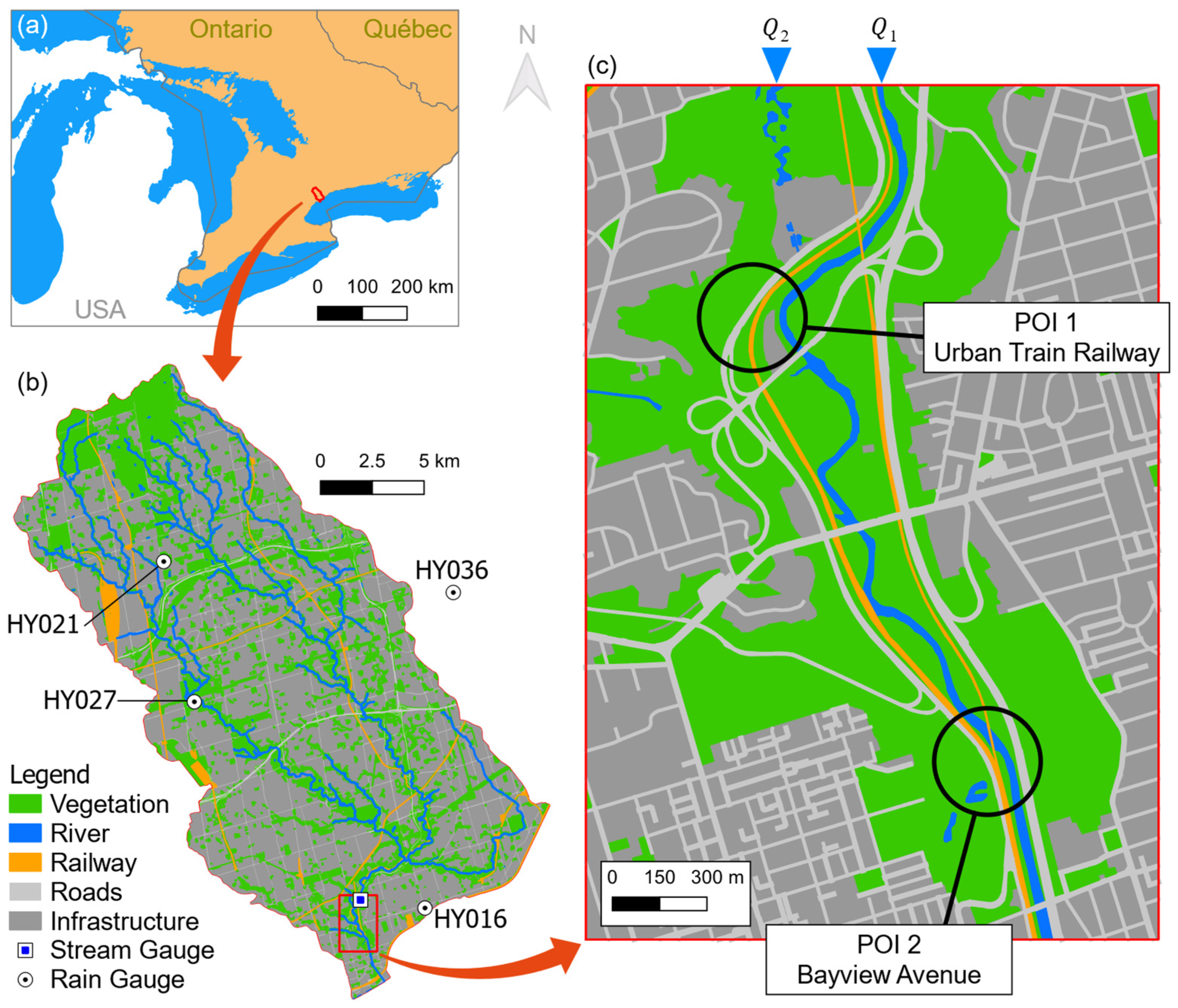
2. Study Area
3. Materials and Methods
3.1. Materials
3.1.1. Data
3.1.2. Hydrodynamic Model
3.2. Methodology Overview
3.3. Setting Up the Ensemble Surrogate Model System (Offline Stage)
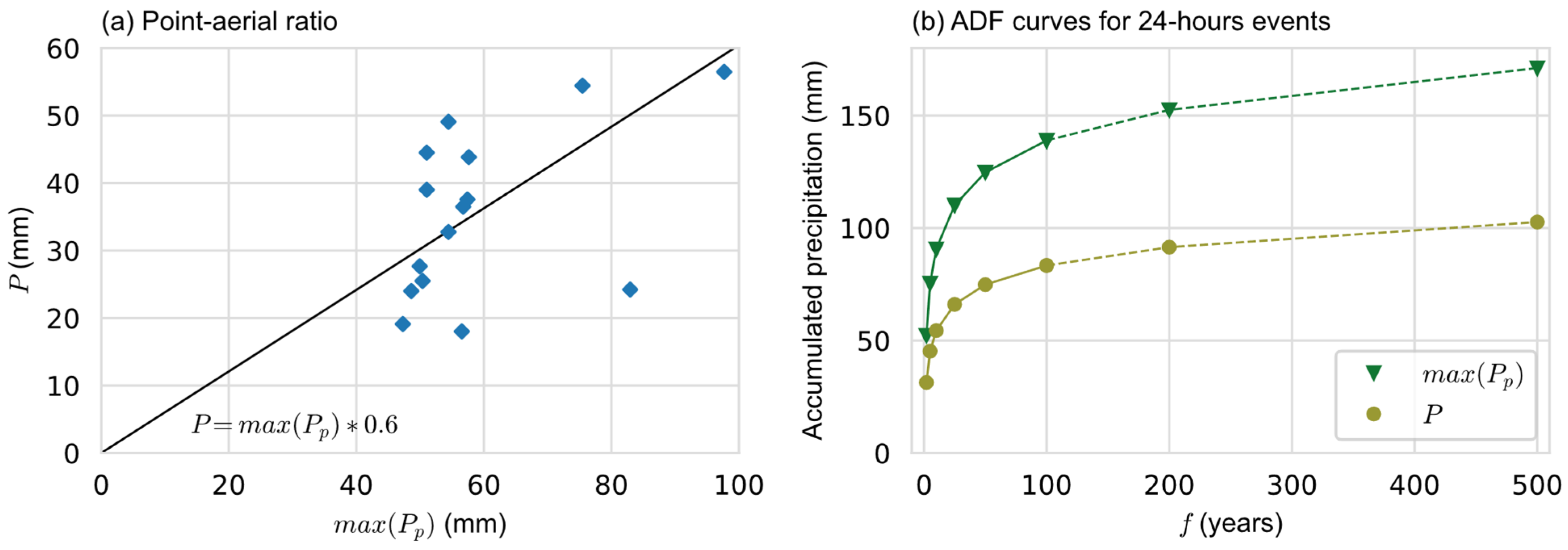
3.3.1. Establishing a Dataset of Significant Rainfall Events
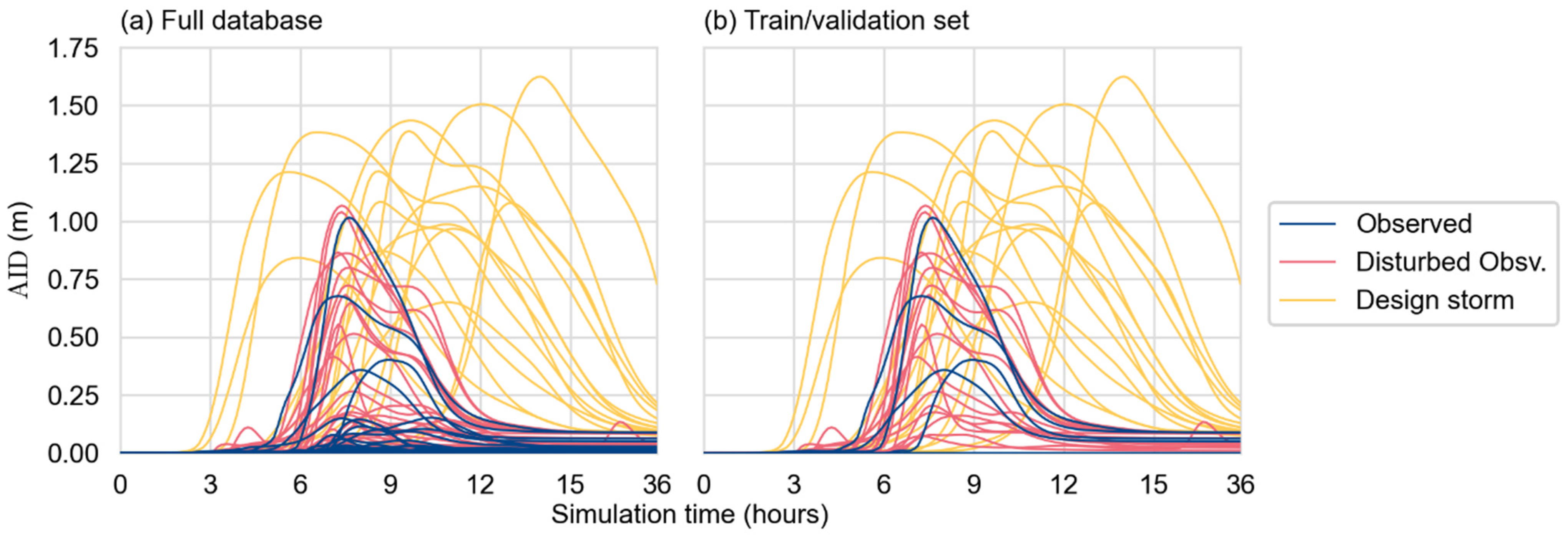
3.3.2. Construction of the Simulations Database
3.3.3. Selection of the Training/Validation and Test Dataset
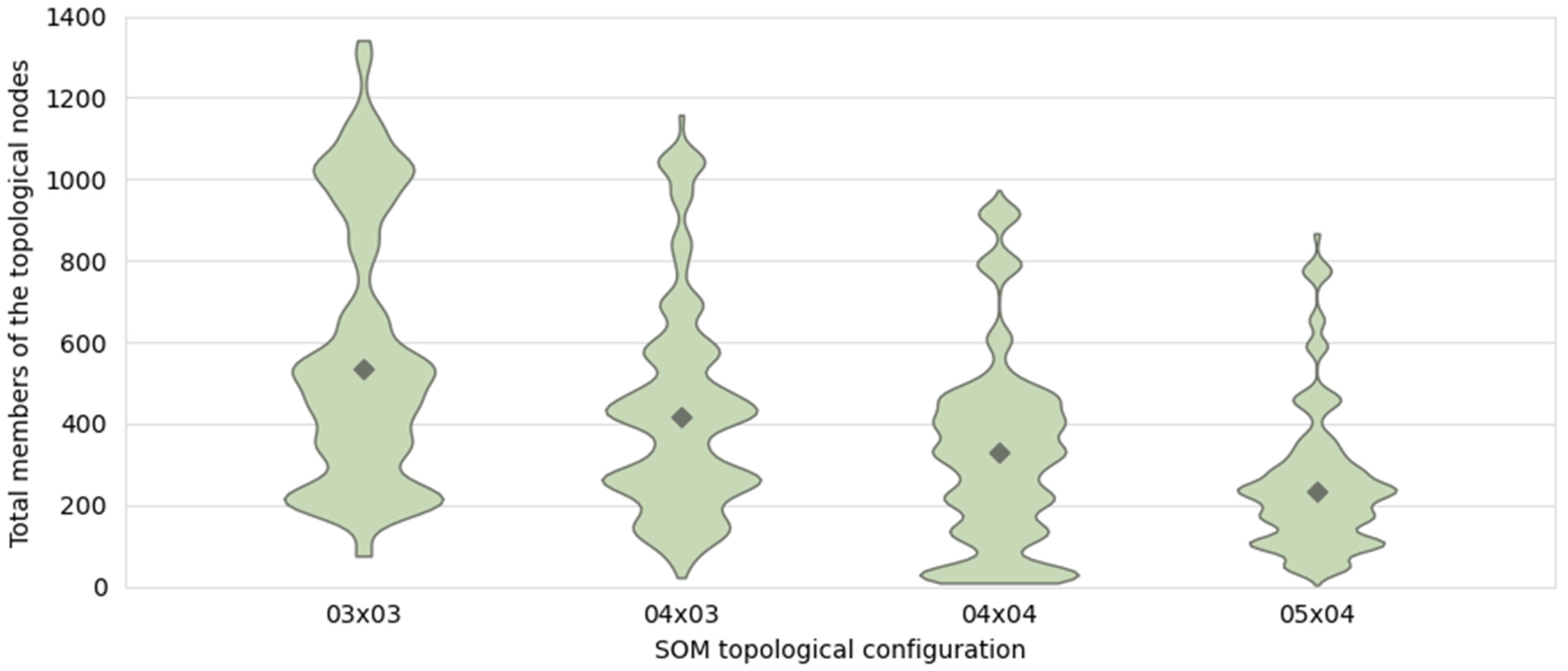
3.3.4. Establishing the Hyperparameters of the Surrogate Models
3.3.5. Training the Surrogate Models
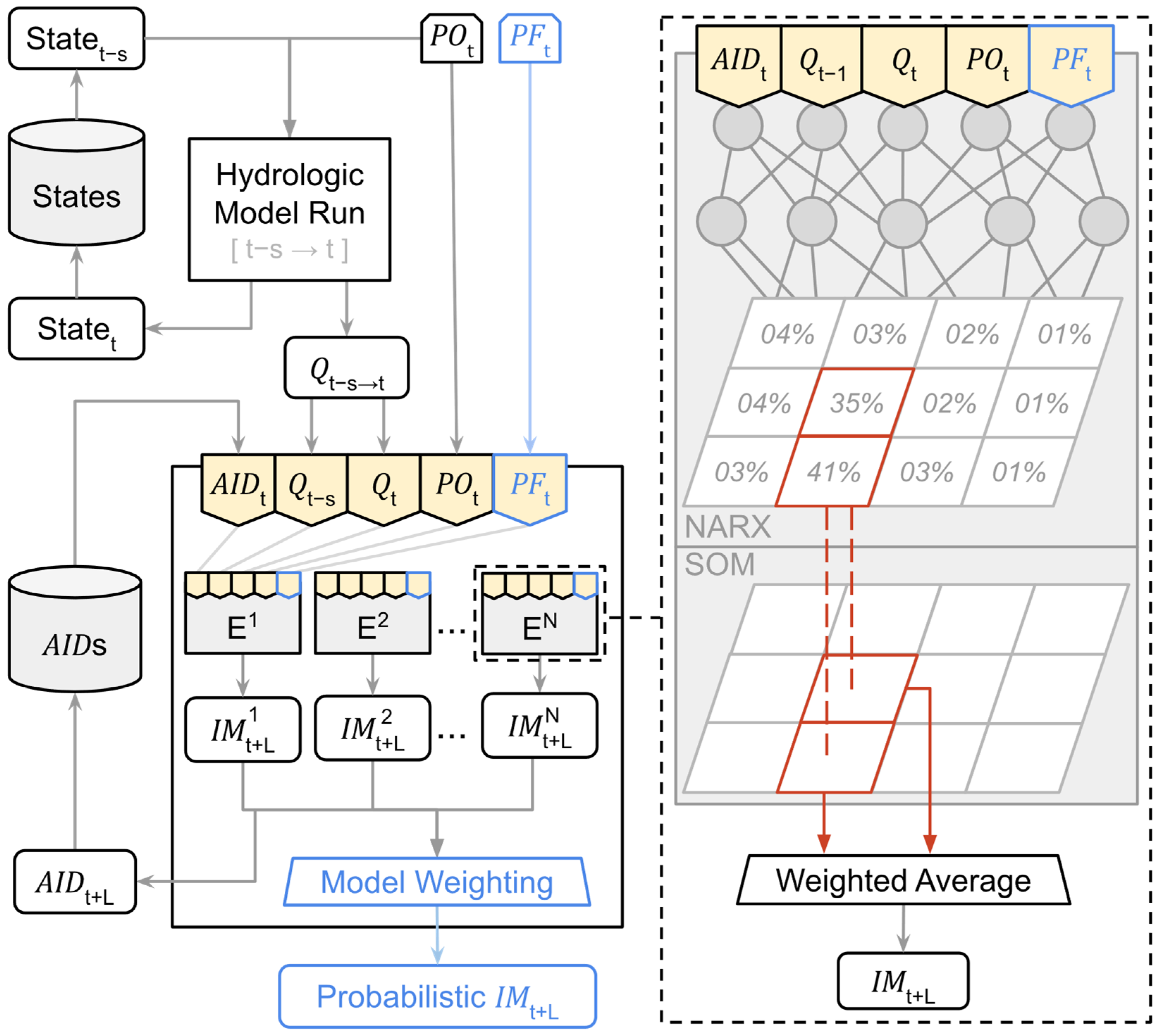
3.4. Forecasting the Probabilistic Inundation Maps
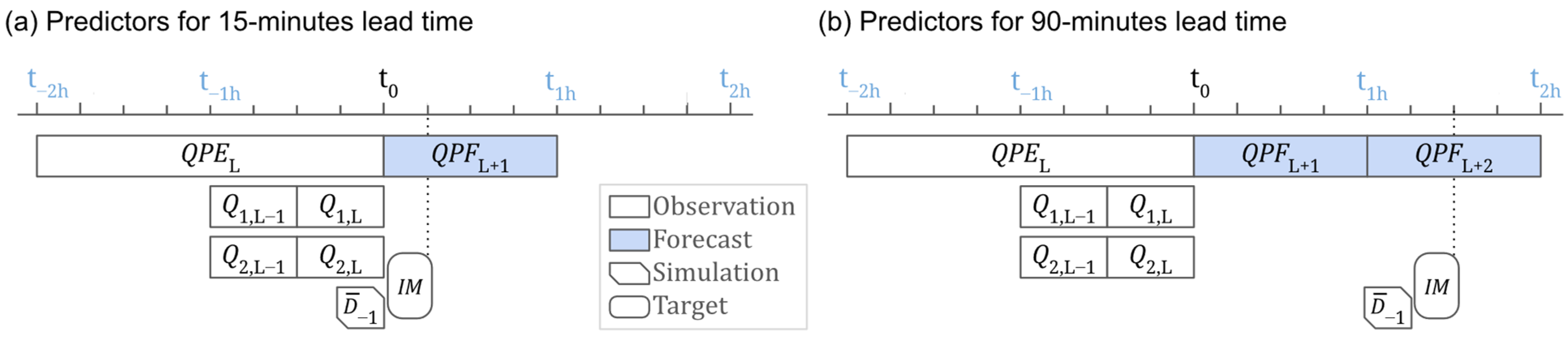
3.4.1. Generating Ensemble Forecasts
3.4.2. Converting Ensembles into Probabilistic Forecasts
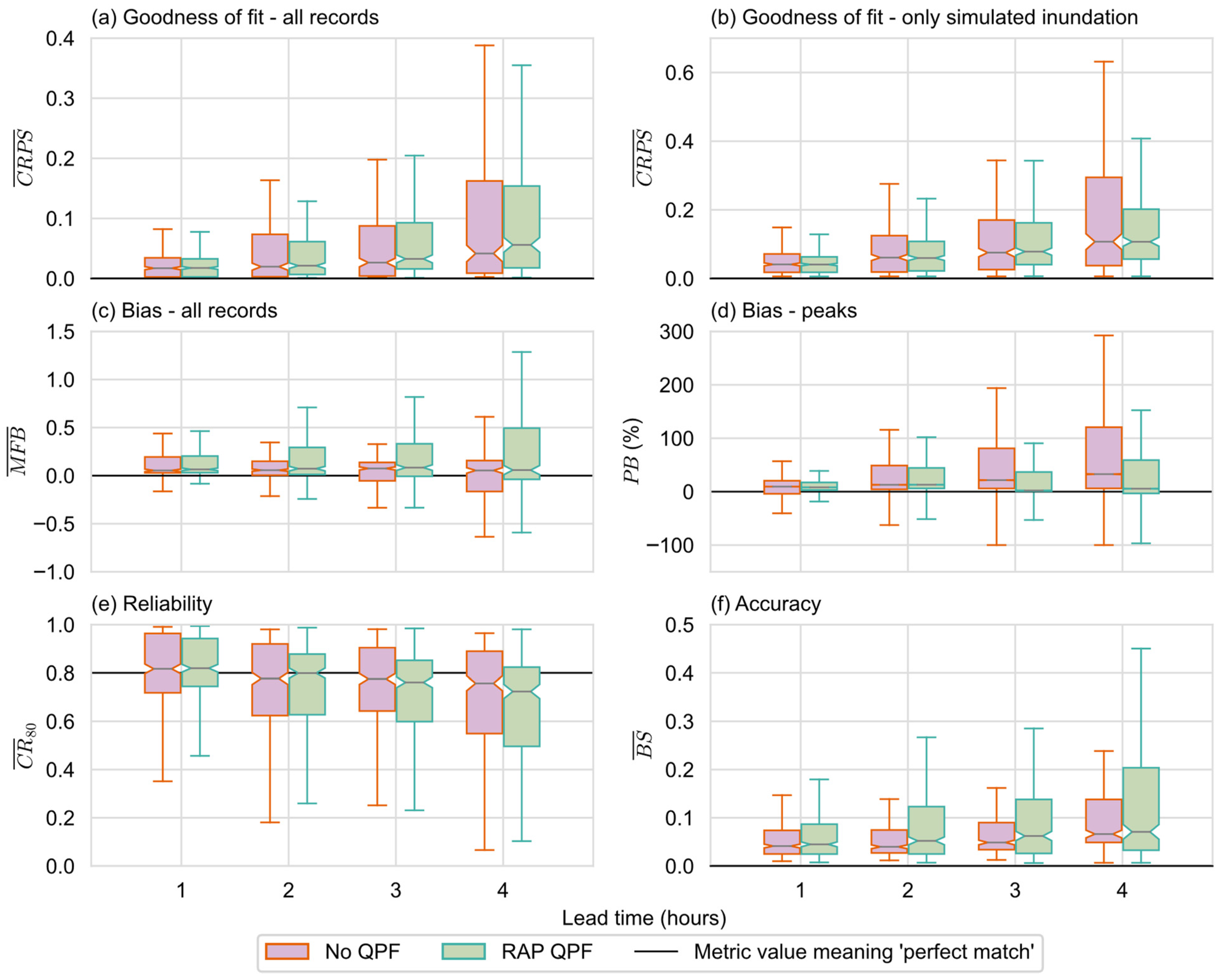
3.5. Evaluation
4. Results and Discussion
4.1. Overall Performance
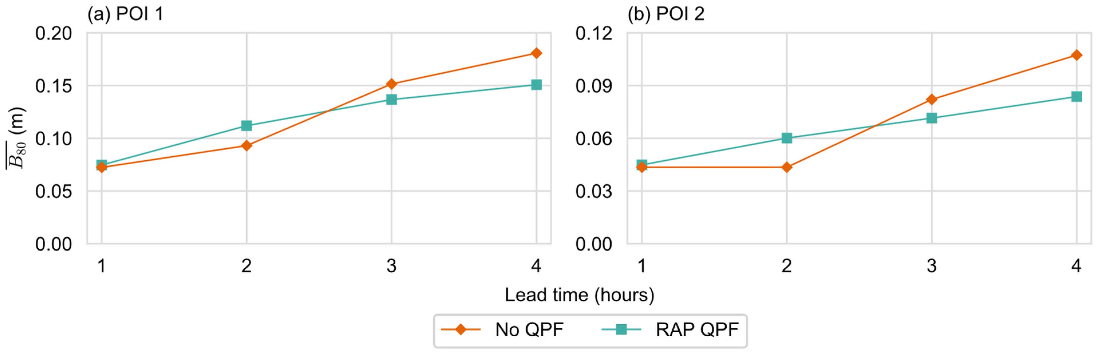
4.2. Study Cases
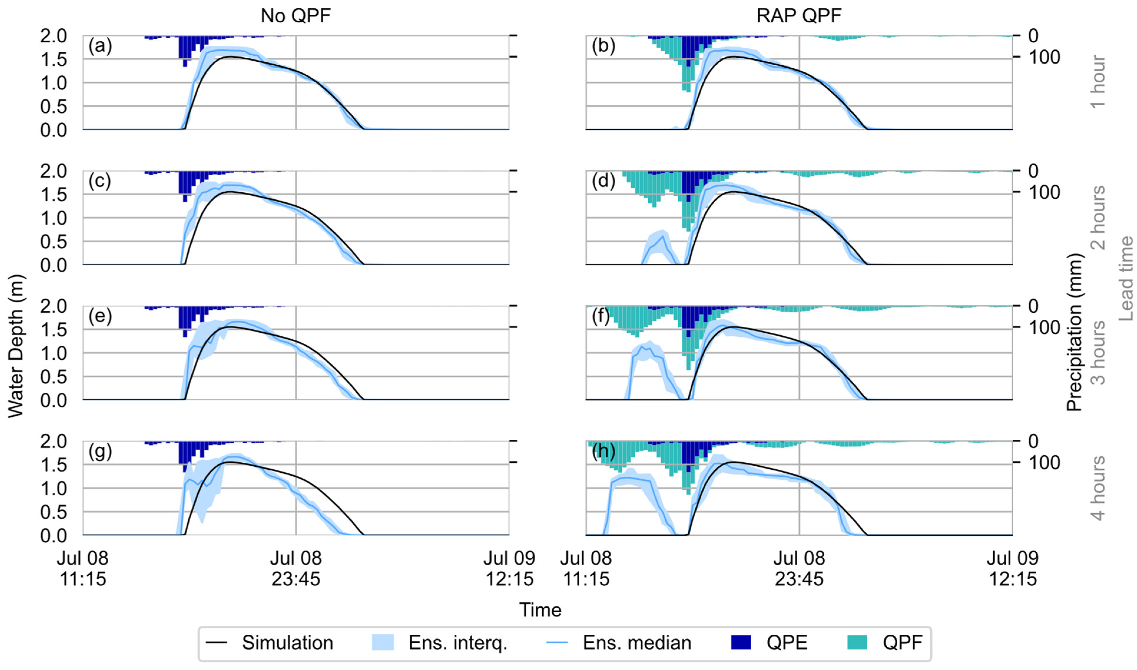
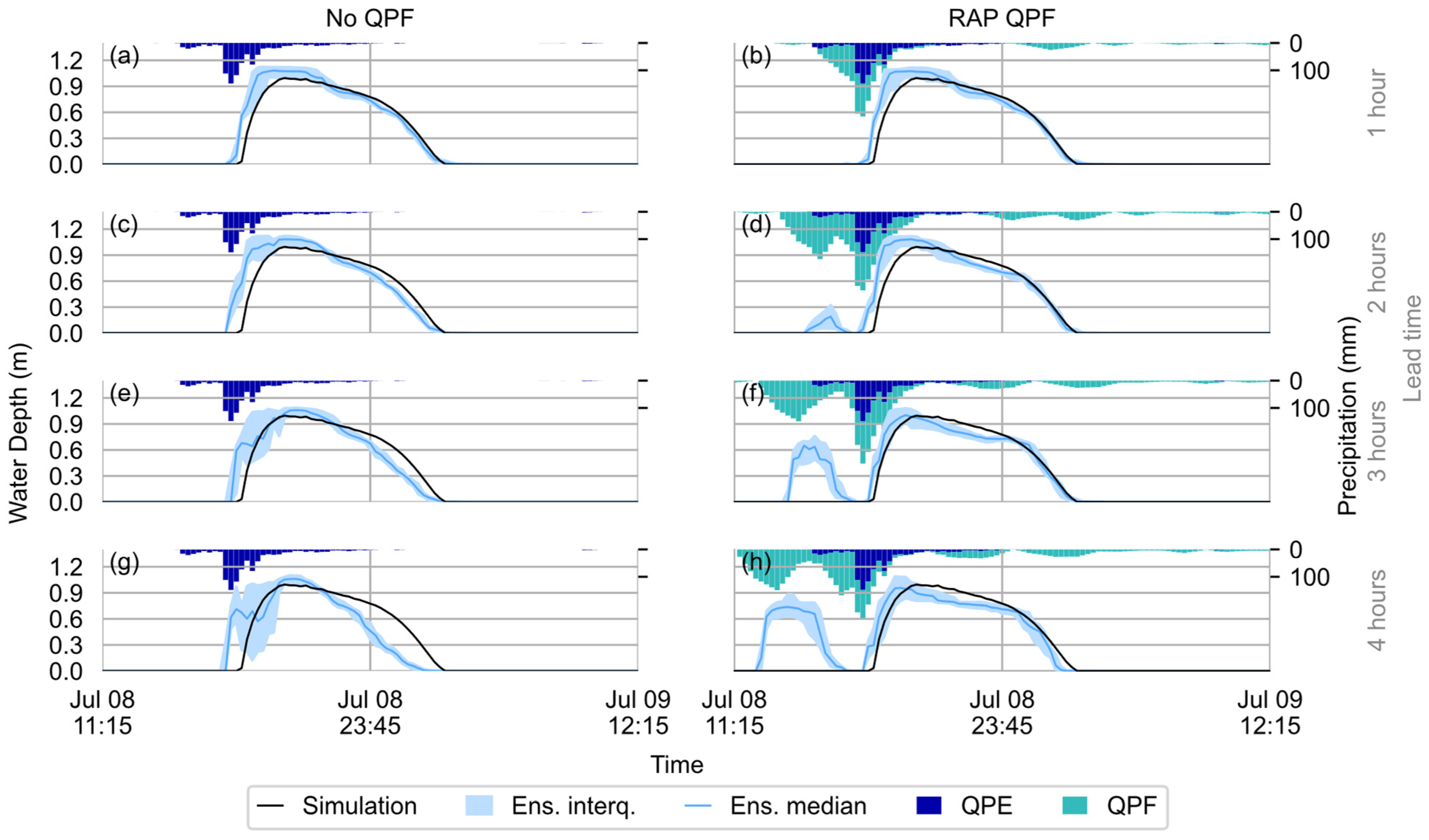
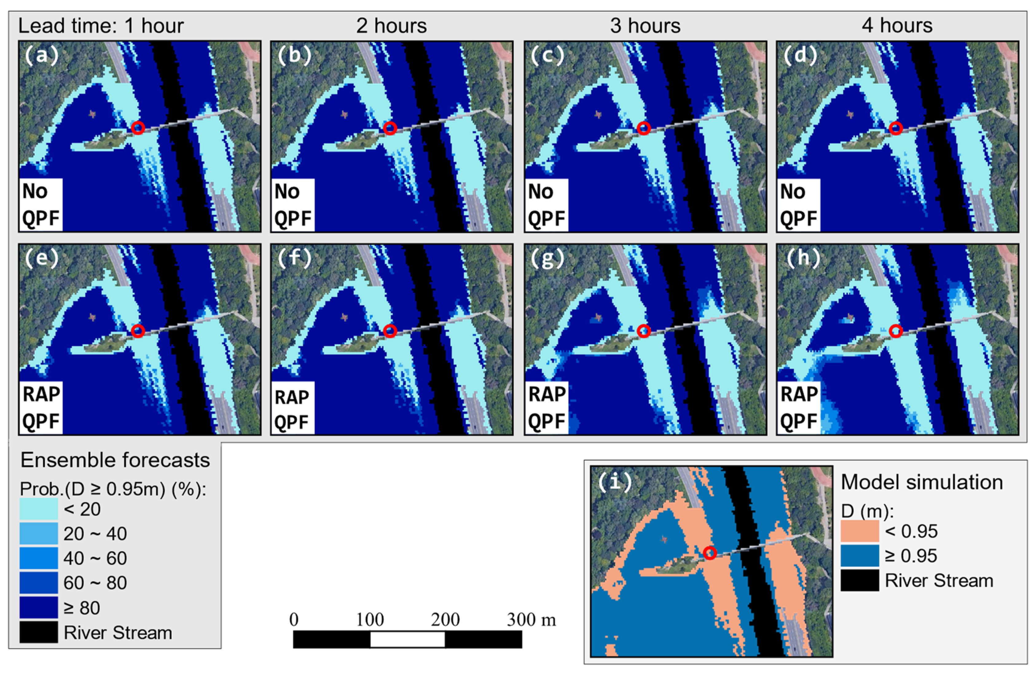
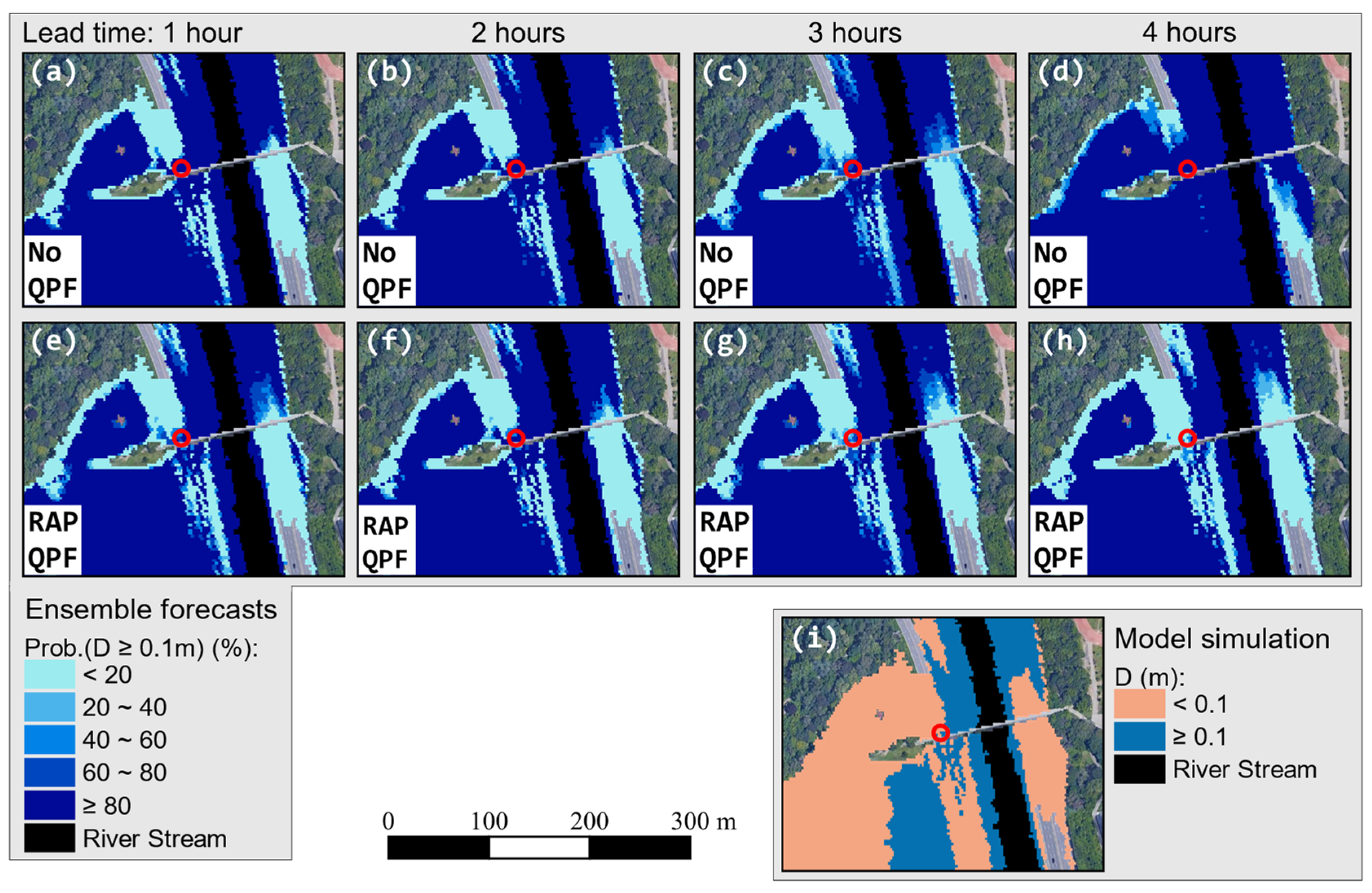
4.2.1. 8 July 2013
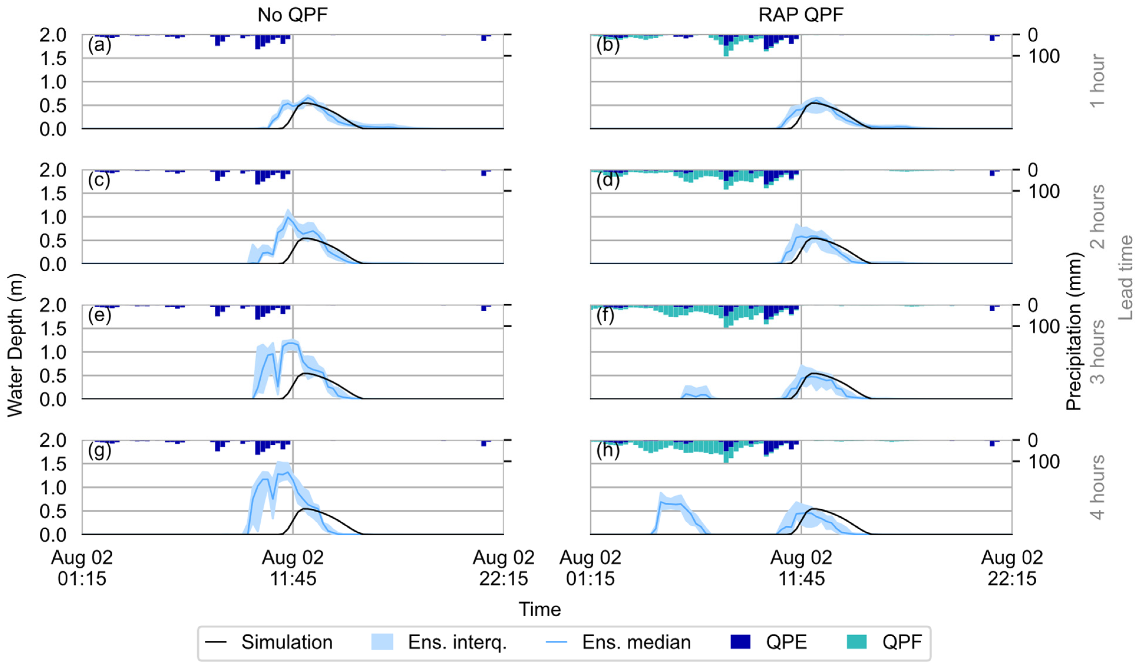
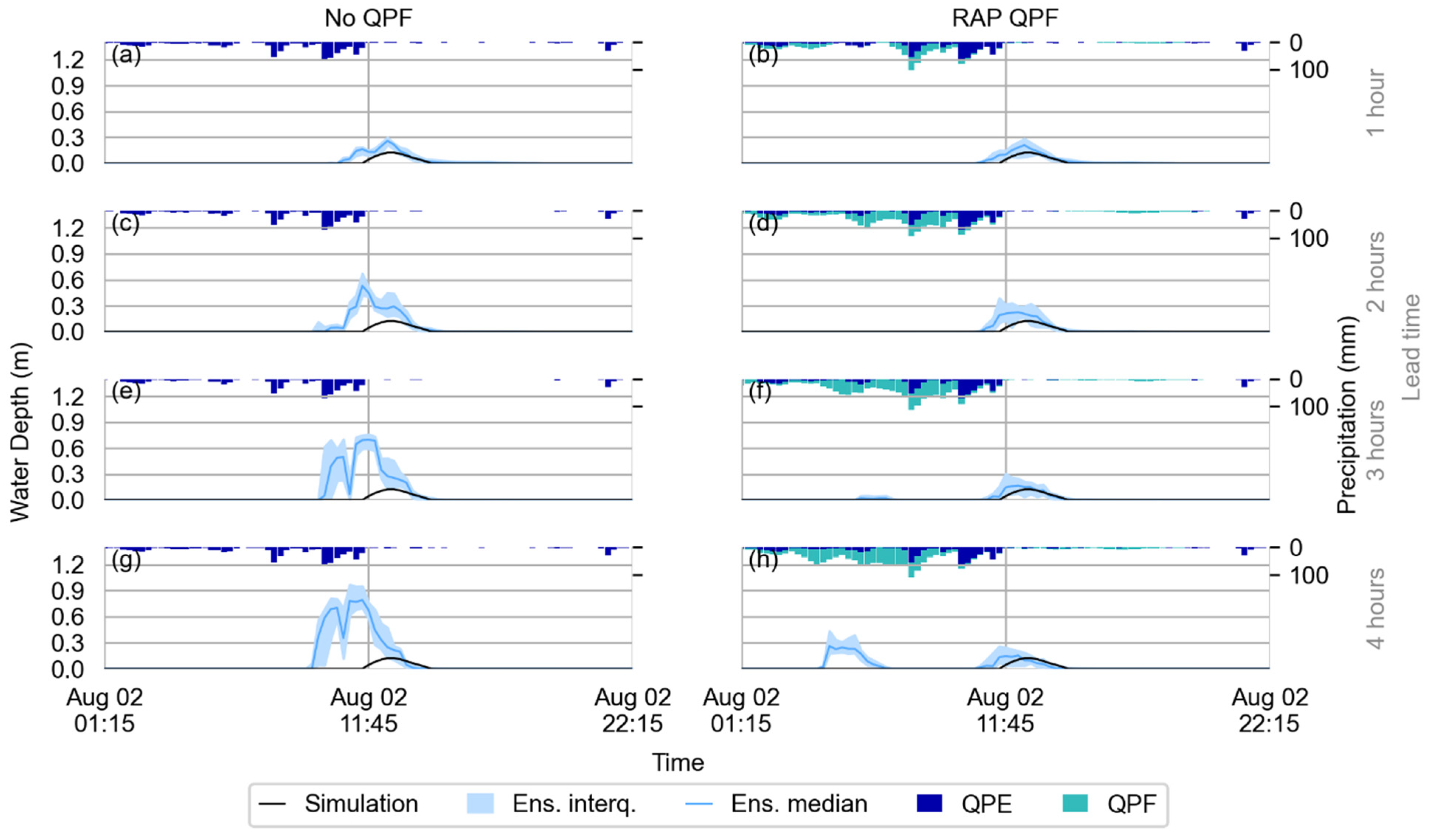
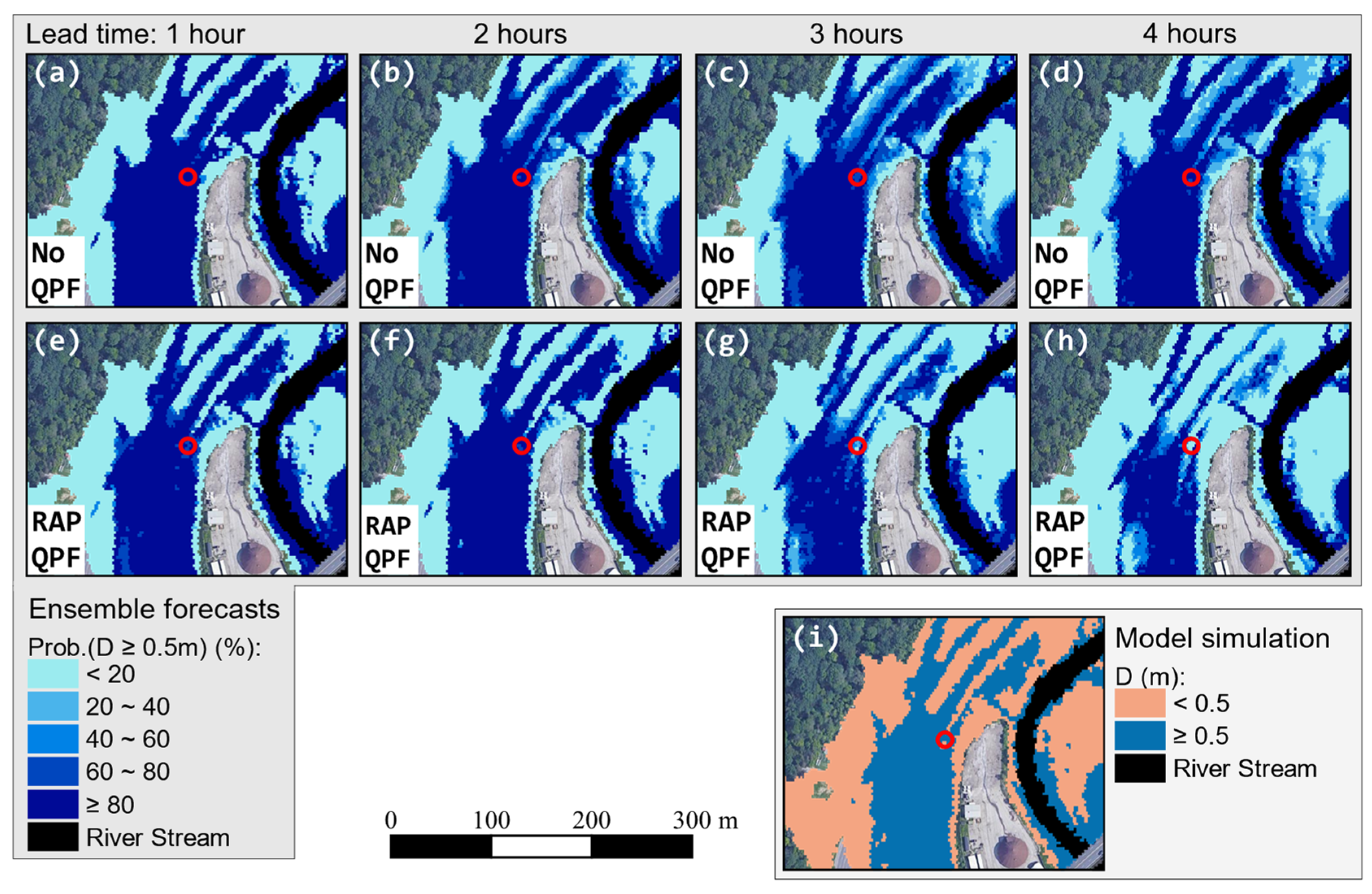
4.2.2. 2 August 2020
4.3. Discussion Summary
4.4. Runtime
5. Conclusions, Limitations, and Future Works
Author Contributions
Funding
Data Availability Statement
Acknowledgments
Conflicts of Interest
Abbreviations
| Acronym | Meaning |
| 2D | Two-dimensional |
| ADF | Accumulation-Duration-Frequency |
| AID | Average Inundation Depth |
| ARF | Aerial Reduction Factor |
| Bα | Bandwidth of α confidence interval |
| BS | Brier Score |
| CADEX | Computer Aided Design of Experiments |
| CRα | Containing Ratio of α confidence interval |
| CRPS | Continuous Ranked Probability Score |
| DEM | Digital Elevation Model |
| ECCC | Environment and Climate Change Canada |
| GRU | Gated Recurrent Unit |
| IDF | Intensity-Duration-Frequency |
| IM | Inundations Map |
| LSTM | Long Short-Term Memory |
| MFB | Mean Fractional Bias |
| NARX | Nonlinear Autoregressive Recurrent Networks with eXogenous inputs |
| POI | Points of Interest |
| QPE | Quantitative Precipitation Estimate |
| QPF | Quantitative Precipitation Forecasts |
| PB | Peak Bias |
| RAM | Random-Access Memory |
| RAP | Rapid Refresh system |
| SOM | Self-Organizing Maps |
| SWE | Snow Water Equivalent |
| SWMM | Storm Water Management Model |
| TRCA | Toronto and Region Conservation Authority |
References
- Fofana, M.; Adounkpe, J.; Larbi, I.; Hounkpe, J.; Djan’na Koubodana, H.; Toure, A.; Bokar, H.; Dotse, S.Q.; Limantol, A.M. Urban Flash Flood and Extreme Rainfall Events Trend Analysis in Bamako, Mali. Environ. Chall. 2022, 6, 100449. [Google Scholar] [CrossRef]
- Sofia, G.; Roder, G.; Dalla Fontana, G.; Tarolli, P. Flood Dynamics in Urbanised Landscapes: 100 Years of Climate and Humans’ Interaction. Sci. Rep. 2017, 7, 40527. [Google Scholar] [CrossRef] [PubMed]
- Yang, L.; Smith, J.A.; Wright, D.B.; Baeck, M.L.; Villarini, G.; Tian, F.; Hu, H. Urbanization and Climate Change: An Examination of Nonstationarities in Urban Flooding. J. Hydrometeorol. 2013, 14, 1791–1809. [Google Scholar] [CrossRef]
- Zanchetta, A.D.L.; Coulibaly, P. Recent Advances in Real-Time Pluvial Flash Flood Forecasting. Water 2020, 12, 570. [Google Scholar] [CrossRef] [Green Version]
- Teng, J.; Jakeman, A.J.; Vaze, J.; Croke, B.F.W.; Dutta, D.; Kim, S. Flood Inundation Modelling: A Review of Methods, Recent Advances and Uncertainty Analysis. Environ. Model. Softw. 2017, 90, 201–216. [Google Scholar] [CrossRef]
- Kaya, C.M.; Tayfur, G.; Gungor, O. Predicting Flood Plain Inundation for Natural Channels Having No Upstream Gauged Stations. J. Water Clim. Change 2019, 10, 360–372. [Google Scholar] [CrossRef] [Green Version]
- Zarzar, C.M.; Hosseiny, H.; Siddique, R.; Gomez, M.; Smith, V.; Mejia, A.; Dyer, J. A Hydraulic MultiModel Ensemble Framework for Visualizing Flood Inundation Uncertainty. J. Am. Water Resour. Assoc. 2018, 54, 807–819. [Google Scholar] [CrossRef]
- Aureli, F.; Prost, F.; Vacondio, R.; Dazzi, S.; Ferrari, A. A GPU-Accelerated Shallow-Water Scheme for Surface Runoff Simulations. Water 2020, 12, 637. [Google Scholar] [CrossRef] [Green Version]
- Ming, X.; Liang, Q.; Xia, X.; Li, D.; Fowler, H.J. Real-Time Flood Forecasting Based on a High-Performance 2-D Hydrodynamic Model and Numerical Weather Predictions. Water Resour. Res. 2020, 56, e2019WR025583. [Google Scholar] [CrossRef]
- Morsy, M.M.; Goodall, J.L.; O’Neil, G.L.; Sadler, J.M.; Voce, D.; Hassan, G.; Huxley, C. A Cloud-Based Flood Warning System for Forecasting Impacts to Transportation Infrastructure Systems. Environ. Model. Softw. 2018, 107, 231–244. [Google Scholar] [CrossRef]
- Bhola, P.K.; Leandro, J.; Disse, M. Framework for Offline Flood Inundation Forecasts for Two-Dimensional Hydrodynamic Models. Geosciences 2018, 8, 346. [Google Scholar] [CrossRef] [Green Version]
- Crotti, G.; Leandro, J.; Bhola, P.K. A 2D Real-Time Flood Forecast Framework Based on a Hybrid Historical and Synthetic Runoff Database. Water 2020, 12, 114. [Google Scholar] [CrossRef] [Green Version]
- Ying, X. An Overview of Overfitting and Its Solutions. J. Phys. Conf. Ser. 2019, 1168, 022022. [Google Scholar] [CrossRef]
- Bermúdez, M.; Cea, L.; Puertas, J. A Rapid Flood Inundation Model for Hazard Mapping Based on Least Squares Support Vector Machine Regression. J. Flood Risk Manag. 2019, 12, 1–14. [Google Scholar] [CrossRef] [Green Version]
- Berkhahn, S.; Fuchs, L.; Neuweiler, I. An Ensemble Neural Network Model for Real-Time Prediction of Urban Floods. J. Hydrol. 2019, 575, 743–754. [Google Scholar] [CrossRef]
- Chang, L.-C.; Amin, M.; Yang, S.-N.; Chang, F.-J. Building ANN-Based Regional Multi-Step-Ahead Flood Inundation Forecast Models. Water 2018, 10, 1283. [Google Scholar] [CrossRef] [Green Version]
- Kim, H.I.; Keum, H.J.; Han, K.Y. Real-Time Urban Inundation Prediction Combining Hydraulic and Probabilistic Methods. Water 2019, 11, 293. [Google Scholar] [CrossRef] [Green Version]
- Kim, H.I.; Han, K.Y. Data-Driven Approach for the Rapid Simulation of Urban Flood Prediction. KSCE J. Civ. Eng. 2020, 24, 1932–1943. [Google Scholar] [CrossRef]
- Zanchetta, A.D.L.; Coulibaly, P. Hybrid Surrogate Model for Timely Prediction of Flash Flood Inundation Maps Caused by Rapid River Overflow. Forecasting 2022, 4, 126–148. [Google Scholar] [CrossRef]
- Bales, J.D.; Wagner, C.R. Sources of Uncertainty in Flood Inundation Maps. J. Flood Risk Manag. 2009, 2, 139–147. [Google Scholar] [CrossRef]
- Zahmatkesh, Z.; Han, S.; Coulibaly, P. Understanding Uncertainty in Probabilistic Floodplain Mapping in the Time of Climate Change. Water 2021, 13, 1248. [Google Scholar] [CrossRef]
- Brandt, S.A. Modeling and Visualizing Uncertainties of Flood Boundary Delineation: Algorithm for Slope and DEM Resolution Dependencies of 1D Hydraulic Models. Stoch. Environ. Res. Risk Assess 2016, 30, 1677–1690. [Google Scholar] [CrossRef] [Green Version]
- Rincón, D.; Khan, U.T.; Armenakis, C. Flood Risk Mapping Using GIS and Multi-Criteria Analysis: A Greater Toronto Area Case Study. Geosciences 2018, 8, 275. [Google Scholar] [CrossRef] [Green Version]
- Krajewski, M.; Brown, D.; Gibbons, E. Flash Flooding, Stormwater, and Decision Making Flash Flooding, Stormwater, and Decision Making for Cities in the Great Lakes; University of Michigan—Climate Center: Ann Arbor, MI, USA, 2015. [Google Scholar]
- Sills, D.; Ashton, A.; Knott, S.; Boodoo, S.; Klaassen, J. A Billion Dollar Flash Flood in Toronto-Challenges for Forecasting and Nowcasting. In Proceedings of the 28th Conference on Severe Local Storms, Portland, OR, USA, 7–11 November 2016. [Google Scholar]
- Benjamin, S.G.; Weygandt, S.S.; Brown, J.M.; Hu, M.; Alexander, C.R.; Smirnova, T.G.; Olson, J.B.; James, E.P.; Dowell, D.C.; Grell, G.A.; et al. A North American Hourly Assimilation and Model Forecast Cycle: The Rapid Refresh. Mon. Weather Rev. 2016, 144, 1669–1694. [Google Scholar] [CrossRef]
- Hapuarachchi, H.A.P.; Wang, Q.J.; Pagano, T.C. A Review of Advances in Flash Flood Forecasting. Hydrol Process. 2011, 25, 2771–2784. [Google Scholar] [CrossRef]
- ECCC-Environment Climate Change Canada Engineering Climate Datasets. Available online: https://climate.weather.gc.ca/prods_servs/engineering_e.html (accessed on 1 May 2022).
- Rossman, L.A. Storm Water Management Model.-User’s Manual Version 5.1; US EPA: Cincinnati, OH, USA, 2015. [Google Scholar]
- Computational Hydraulics International-CHI PCSWMM. Available online: https://www.pcswmm.com/ (accessed on 10 June 2022).
- Dinu, C.; Sîrbu, N.; Drobot, R. Delineation of the Flooded Areas in Urban Environments Based on a Simplified Approach. Appl. Sci. 2022, 12, 3174. [Google Scholar] [CrossRef]
- Huff, F.A. Time Distribution of Rainfall in Heavy Storms. Water Resour Res. 1967, 3, 1007–1019. [Google Scholar] [CrossRef]
- Chow, V.T. Applied Hydrology; Clark, B.J., Morriss, J., Eds.; McGraw-Hill: New York, NY, USA, 1988; ISBN 0 07-010810-2. [Google Scholar]
- Wright, D.B.; Mantilla, R.; Peters-Lidard, C.D. A Remote Sensing-Based Tool for Assessing Rainfall-Driven Hazards. Environ. Model. Softw. 2017, 90, 34–54. [Google Scholar] [CrossRef] [Green Version]
- Kennard, R.W.; Stone, L.A. Computer Aided Design of Experiments. Technometrics 1969, 11, 137. [Google Scholar] [CrossRef]
- Shenk, J.S.; Westerhaus, M.O. Population Definition, Sample Selection, and Calibration Procedures for Near Infrared Reflectance Spectroscopy. Crop. Sci. 1991, 31, 469–474. [Google Scholar] [CrossRef]
- Cook, R.L. Stochastic Sampling in Computer Graphics. ACM Trans. Graph. 1986, 5, 51–72. [Google Scholar] [CrossRef]
- Kohonen, T. Self-Organized Formation of Topologically Correct Feature Maps. Biol. Cybern. 1982, 43, 59–69. [Google Scholar] [CrossRef]
- Kohonen, T. MATLAB Implementations and Applications of the Self-Organizing Map; Unigrafia Oy: Helsinki, Finland, 2014; ISBN 9789526036786. [Google Scholar]
- Xiong, L.; Wan, M.; Wei, X.; O’Conno, K.M. Indices for Assessing the Prediction Bounds of Hydrological Models and Application by Generalised Likelihood Uncertainty Estimation. Hydrol. Sci. J. 2009, 54, 852–871. [Google Scholar] [CrossRef] [Green Version]
- Boylan, J.W.; Russell, A.G. PM and Light Extinction Model Performance Metrics, Goals, and Criteria for Three-Dimensional Air Quality Models. Atmos. Environ. 2006, 40, 4946–4959. [Google Scholar] [CrossRef]
- CBC News. Toronto’s All Wet: Some Images From The Flash Floods That Hit T.O. Last Night. 2013. Available online: https://www.cbc.ca/strombo/news/torontos-all-wet-some-images-from-the-flash-floods-that-hit-to-last-night.h (accessed on 12 September 2022).
- CTV News. What’s Open and Closed This Holiday Monday in Toronto? 2020. Available online: https://toronto.ctvnews.ca/what-s-open-and-closed-this-civic-holiday-monday-in-toronto-1.6008664 (accessed on 12 September 2022).
- DailyHive News. Rain Causes Flooding on Low-Lying Toronto Highway Ramps. 2020. Available online: https://dailyhive.com/toronto/highway-ramp-flooding-rain (accessed on 12 September 2022).
- Burg, T.; Elmore, K.L.; Grams, H.M. Assessing the Skill of Updated Precipitation-Type Diagnostics for the Rapid Refresh with MPING. Weather 2017, 32, 725–732. [Google Scholar] [CrossRef]
- Chen, C.; Jiang, J.; Zhou, Y.; Lv, N.; Liang, X.; Wan, S. An Edge Intelligence Empowered Flooding Process Prediction Using Internet of Things in Smart City. J. Parallel Distrib. Comput. 2022, 165, 66–78. [Google Scholar] [CrossRef]
- Fu, M.; Fan, T.; Ding, Z.; Salih, S.Q.; Al-Ansari, N.; Yaseen, Z.M. Deep Learning Data-Intelligence Model Based on Adjusted Forecasting Window Scale: Application in Daily Streamflow Simulation. IEEE Access 2020, 8, 32632–32651. [Google Scholar] [CrossRef]
- Song, T.; Ding, W.; Wu, J.; Liu, H.; Zhou, H.; Chu, J. Flash Flood Forecasting Based on Long Short-Term Memory Networks. Water 2019, 12, 109. [Google Scholar] [CrossRef] [Green Version]
- Arsenault, R.; Martel, J.; Mai, J. Continuous Streamflow Prediction in Ungauged Basins: Long Short- Term Memory Neural Networks Clearly Outperform Hydrological Models. Hydrol. Earth Syst. Sci. 2022; in review. [Google Scholar] [CrossRef]
- Kilsdonk, R.A.H.; Bomers, A.; Wijnberg, K.M. Predicting Urban Flooding Due to Extreme Precipitation Using a Long Short-Term Memory Neural Network. Hydrology 2022, 9, 105. [Google Scholar] [CrossRef]
- Ghaith, M.; Yosri, A.; El-Dakhakhni, W. Synchronization-Enhanced Deep Learning Early Flood Risk Predictions: The Core of Data-Driven City Digital Twins for Climate Resilience Planning. Water 2022, 14, 3619. [Google Scholar] [CrossRef]
- Mosavi, A.; Ozturk, P.; Chau, K.W. Flood Prediction Using Machine Learning Models: Literature Review. Water 2018, 10, 1536. [Google Scholar] [CrossRef]


| Coefficient | Return Period (Years) | ||||
|---|---|---|---|---|---|
| 25 | 50 | 100 | 200 | 500 | |
| 41.0 | 46.0 | 50.9 | 55.7 | 61.9 | |
| −0.689 | −0.686 | −0.684 | −0.683 | −0.680 | |
| Type of Precipitation | ||||
|---|---|---|---|---|
| Set of Simulations | Observed | Disturbed Observation | Design Storm | Total |
| Full database | 31 | 62 | 15 | 108 |
| Training/Validation | 5 | 16 | 15 | 36 |
| Predictor | Meaning | On Lead Time L |
|---|---|---|
| Mean estimated precipitation, 2-h accumulation | All | |
| Earlier inflow discharge at , 30-min mean | All | |
| Later inflow discharge at , 30-min mean | All | |
| Earlier inflow discharge at , 30-min mean | All | |
| Later inflow discharge at , 30-min mean | All | |
| (or ) | Average antecedent simulated inundated depth, instant | All |
| Mean predicted forecast, 1-h accumulation, 1 h ahead | All | |
| Mean predicted forecast, 1-h accumulation, 2 h ahead | L > 60 min | |
| Mean predicted forecast, 1-h accumulation, 3 h ahead | L > 120 min | |
| Mean predicted forecast, 1-h accumulation, 4 h ahead | L > 180 min |
| Lead Time (h) | |||||
|---|---|---|---|---|---|
| Number of Folds | 1 | 2 | 3 | 4 | Mean |
| 04 | 0.026 | 0.030 | 0.034 | 0.032 | 0.030 |
| 06 | 0.033 | 0.029 | 0.029 | 0.029 | 0.030 |
| 09 | 0.026 | 0.034 | 0.042 | 0.049 | 0.038 |
| 12 | 0.021 | 0.023 | 0.026 | 0.029 | 0.024 |
| 18 | 0.021 | 0.027 | 0.031 | 0.032 | 0.028 |
Publisher’s Note: MDPI stays neutral with regard to jurisdictional claims in published maps and institutional affiliations. |
© 2022 by the authors. Licensee MDPI, Basel, Switzerland. This article is an open access article distributed under the terms and conditions of the Creative Commons Attribution (CC BY) license (https://creativecommons.org/licenses/by/4.0/).
Share and Cite
Zanchetta, A.D.L.; Coulibaly, P. Probabilistic Forecasts of Flood Inundation Maps Using Surrogate Models. Geosciences 2022, 12, 426. https://doi.org/10.3390/geosciences12110426
Zanchetta ADL, Coulibaly P. Probabilistic Forecasts of Flood Inundation Maps Using Surrogate Models. Geosciences. 2022; 12(11):426. https://doi.org/10.3390/geosciences12110426
Chicago/Turabian StyleZanchetta, Andre D. L., and Paulin Coulibaly. 2022. "Probabilistic Forecasts of Flood Inundation Maps Using Surrogate Models" Geosciences 12, no. 11: 426. https://doi.org/10.3390/geosciences12110426