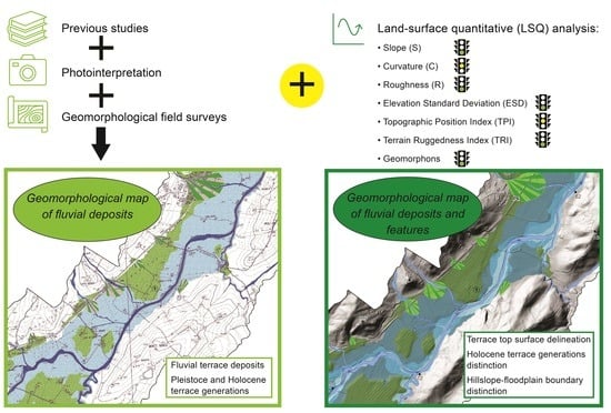
1. Introduction
Fluvial deposits provide one of the most-studied continental records of climate changes, and consequently, fluvial terraces represent important geomorphological features in diverse morphoclimatic contexts worldwide [
1]. There is now a wide consensus on the role of climate variability in producing alternation in the fluvial incision and sedimentation processes recorded in fluvial terraces [
2,
3]. Therefore, the cyclical interchange between the erosional and depositional processes during quaternary can be considered the main response of fluvial systems to climate change [
1]. Further, many studies have demonstrated that fluvial terrace staircases are responses to regional uplift at a long time scale (10
4–10
6 year) [
4]. Therefore, the sensitivity of fluvial dynamics to tectonics and climate variability allows for the use of geomorphic and stratigraphic records as quantitative archives of past climatic conditions and tectonics.
Focusing on the last glacial–interglacial cycle, the fluvial sequence is often represented by several fill-cut episodes, which have formed two/three (or more) terrace steps since the last glacial maximum during the Holocene [
5,
6]. Minor aggradation phases along the inner valley sectors from the Holocene can be recognized at several places in the world. These phases are often accelerated either by increased mass wasting along hillslopes or by anthropogenic soil erosion. Although the late glacial and Holocene terrace sequences are among the best studied and exposed alluvial records worldwide, their complexity and intriguing arrangement stimulates further research perspectives aimed at unraveling the types and ages as well as the altimetric arrangement and along-valley distribution. Indeed, the late glacial and Holocene terrace sequences are often dissimilar not only because of the diverse morphoclimatic and geodynamic contexts, but even along adjacent valleys in the same region.
Along the river valleys draining the Adriatic side of the northern Marche Apennines (
Figure 1), a late Pleistocene-to-Holocene terrace sequence constitutes the present valley floors hanging from a few meters up to maximum of 18–20 m above the thalweg. Even though mapping fluvial terraces in the field is a standard geomorphological procedure, over wide and low-relief floodplains, traditional geomorphological mapping is particularly challenging [
7], as is the case along the valley floors within the northern Marche Apennines [
8]. In facts, the difficulty of detecting Holocene fluvial terraces in the field, as well as distinguishing the latter from the ancient late Pleistocene terrace generation, has many origins, including (i) the size of the terrace surfaces, often too large to be completely seen in the field, and (ii) the subjectivity of the examiner in detecting all terrace features and their geometric and geomorphological characteristics (e.g., external scarp, inner edge, lateral edges, basal strath, deposit thickness and composition, and terrace surface) with adequate accuracy and detail. From this perspective, fluvial terraces exposed along the northern Marche river valleys are ideal for testing a geomorphological approach to enhancing the detection and interpretation of fluvial terraces and better comprehending their morpho-evolutive implications.
The introduction of digital terrain models (DTMs) has provided a great opportunity for the remote analysis of terrace morphology and surficial geometry using geographic information systems (GIS). Different efforts have been carried out over the course of the last twenty years for the automatic extraction of terrace features, such as terrace surfaces or terrace scarps, using low-resolution interpolated DTMs [
9] and high-resolution DTMs derived from light detection and ranging (LiDAR) [
10,
11]. Automated methods for the extraction of fluvial terraces have proven to be supportive in different contexts, and they have often been often for extracting terrace features, even where terrace remnants were scarcely observable [
12]. Nonetheless, the analysis of late Pleistocene–Holocene floodplains, characterized by a very complex spatial arrangement of terrace morphology and structure, can be difficult to perform, and the purely automatic detection of terrace features is challenging. Therefore, a great opportunity is offered by the combination of land-surface quantitative (LSQ) analysis based on high-resolution DTMs with ground-truth geomorphological investigations, which have proven to be effective for the analysis of Earth surface processes and landforms at different space–time scales [
6,
13,
14,
15].
In this work, a combined approach is presented for the identification and mapping of the late Pleistocene–Holocene fluvial terraces exposed along the mid sector of the Misa River valley. This approach is based on geomorphological field surveys and mapping combined with the computation and assessment of different morphometric parameters (local, statistical, and object-based). These parameters have been calculated from high-resolution DTM derived from LiDAR surveys conducted in the frame of the national project called “Not Ordinary Plan of Remote Sensing” [
16]. After a short presentation of the study area and the exhibition of the complete methodological approach, the main results are presented, and their general methodological implications are discussed together with site-specific geomorphological findings and implications.
Figure 1.
Geological sketch, derived from a geo-lithological map of Italy [
17], of the northern Marche Apennines, encompassing the study area. In the mainframe: 1. River; 2. Coastline; 3. Pleistocene and Holocene fluvial deposits; 4. Plio-Pleistocene sands and conglomerates; 5. Plio-Pleistocene clays; 6. Miocene marly-calcareous, evaporitic, and terrigenous unit; 7. Mesozoic limestones. In the top left corner: the location of the study area in the Italian peninsula. Coordinate references are provided in World Geodetic System (WGS) 1984, Universal Transverse Mercator (UTM) Zone 32N (EPSG: 32632).
2. Study Area
The northern Marche Apennines consist of an inner, mainly mountainous area merging to the NE into a hilly coastal zone (
Figure 1), the latter developing for about 65 km along the western side of the central Adriatic Sea. The first area pertains to the Meso-Cenozoic carbonatic and marly-carbonatic, autochthonous Umbria–Marche geological domain, while the latter zone is shaped from Neogene terrigenous formations. The inland Umbria–Marche domain is characterized by two regionally extended anticlines (i.e., the Umbria–Marche Ridge to the SW and the Marche Ridge to the SE), separated by a broad, mainly terrigenous syncline where several minor carbonate anticlines also rise. The fold shape is typically imprinted on the planform of the derived sub-parallel, NW–SE-trending morphostructures (
Figure 1).
Tectonic uplift rates over the last 1 Ma have been estimated to be comprised of between 0.3 and 0.5 mm/year in the inner sectors of the chain, and between 0.15 and 0.18 mm/year along the Adriatic coastal sectors [
8].
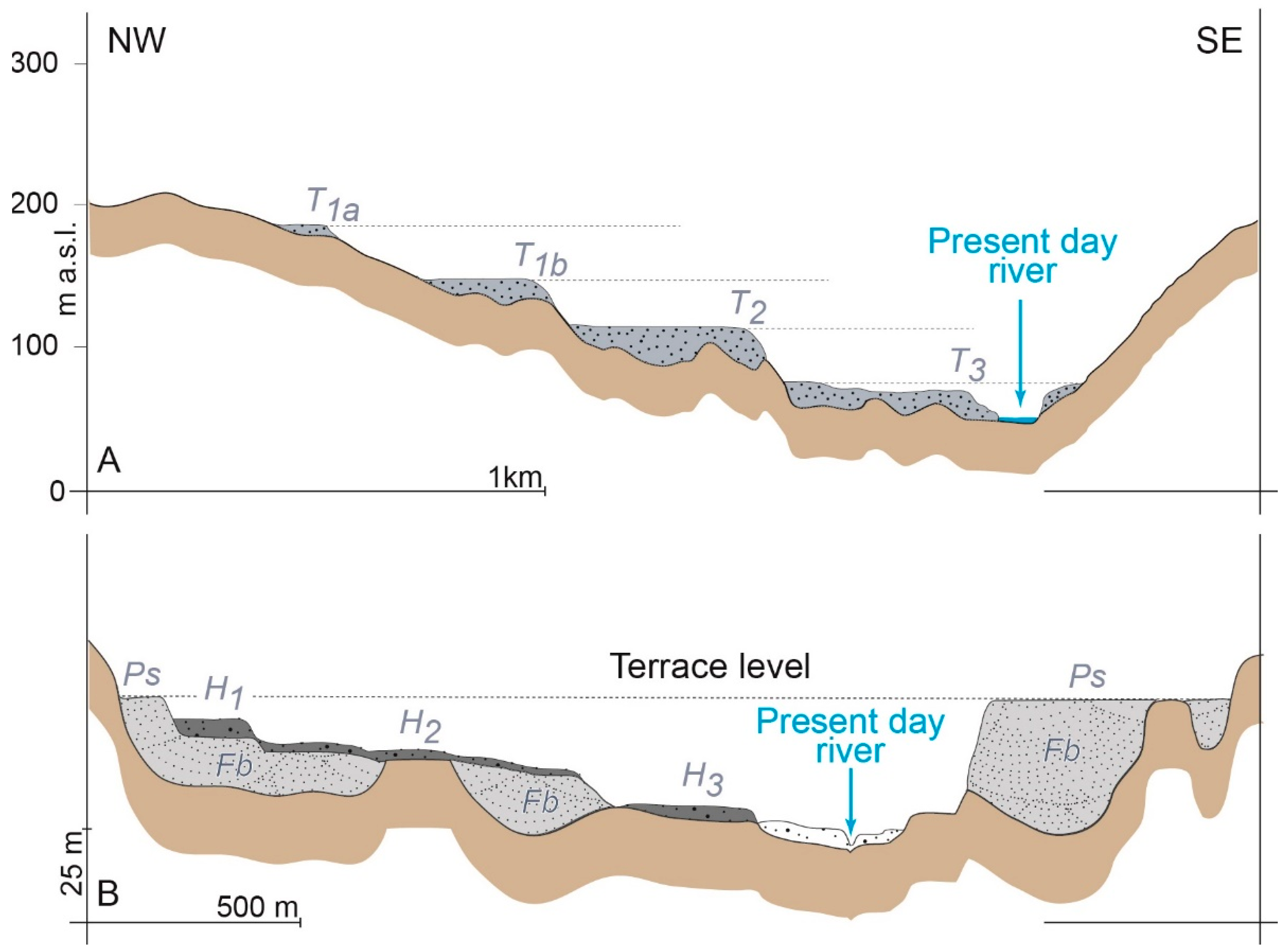
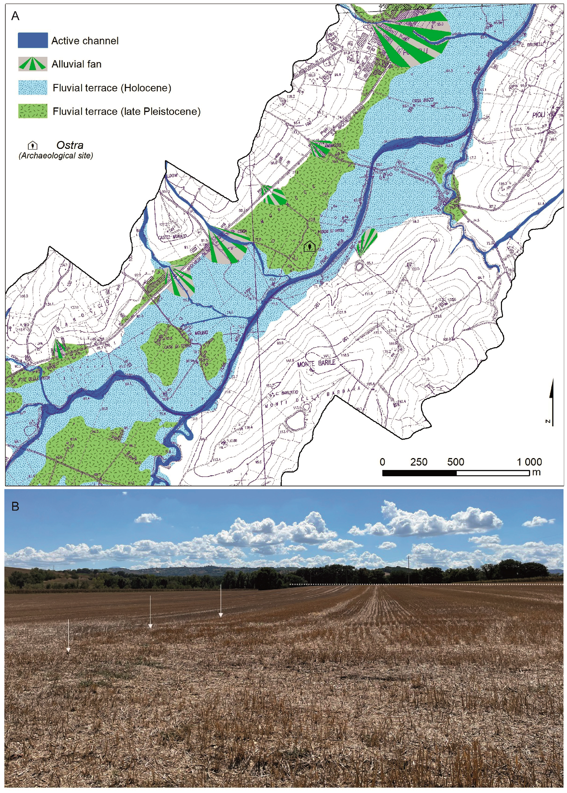
The main watercourses mostly drain eastward, cross cutting the main geological structures and forming sub-parallel valleys. The last ones, along their middle and lowermost sectors expose a well-preserved terrace staircase hanging at different heights along the valley sides and flat floodplains up to 2–4 km wide (
Figure 2A). Floodplains typically enlarge in proximity of the river mouths, showing bell-shaped planforms that have been interpreted by [
18] as the surficial expression of wide coastal fan bodies developed during the last sea level rise but still under low stand conditions in the late Pleistocene–early Holocene. The complex arrangement of the fluvial terrace staircase has been widely studied and discussed in the past (see the works by [
19,
20]). In general, up to ten levels compose an ideal fluvial terraces staircase, which, as a rule, starts with the remnants of ancient strath terraces. These hang at heights above the present thalweg higher than 150–180 m, and their origin has widely been accepted to be related to tectonic uplift [20 and references therein]. The fill terraces sequence is mainly represented by remnants of up to five generations of gravel-dominated terraces, from middle-Pleistocene to Holocene in age, hanging at heights above the thalweg from a few of meters up to 120–150 m, named, from the ancient ones, T1a-1b, T2, T3, and T4 (
Figure 2A). This latter is a complex series of nested minor terrace levels formed during a general post-glacial downcutting phase [
18,
19,
20] (
Figure 2B). Late Quaternary climate changes, in a context of active regional tectonic uplift, principally accounts for the genesis and development of different fill terrace generations. During the Pleistocene, the northern Marche inland was glacier-free, therefore the influence of small local glaciers on fluvial terraces’ development must be considered as irrelevant [
20]. The terrace deposits belonging to the different generations are generally composed of a fluvial depositional sequence that starts at the base with thick gravels and sands of braided-type river channels, representing the main alluvial infilling during glacial cold conditions, which often superimposes late-glacial alluvial fan deposits [
21]. These latter show different thickness, with maxima at the tributary junctions, and represent the termination of the depositional phase of each terrace generation, especially the ancient ones, after which the valley entrenchment started. This cyclical deposition pattern principally characterizes the highest, ancient depositional terrace generations (i.e., T1a–1b, T2, and, partially, T3), being an exception the youngest terrace generation starting from the T3 [
20,
22,
23,
24] (
Figure 2B). Moreover, the late Pleistocene–Holocene terrace is characterized by a series of sub-horizontal terrace treads, slightly dipping towards the present channel, separated by minor terrace scarps (with heights often less than 2–3 m), which are often slightly convex slope breaks remolded by shallow mass movements and surficial running waters. The present floodplains, composed by these terrace generations, are often covered by patches of arboreal and shrubby vegetation, hosting intense agricultural practices and deep anthropogenic changes since the first urbanization of the area as far back as the Roman times [
25]. In fact, the current valley floors host several Roman archeological sites and connected structures. The ancient Ostra Roman village along the Misa River, as well as the Forum Sepronii along the Metauro River and the ancient Suasa Roman village along the Cesano River, developed above the T3 terrace surface or immediately below along the inner margin of the Holocene minor terrace levels, indicating complex interrelations between early human occupation and the watercourses [
24,
25].
3. Materials and Methods
The available datasets on fluvial terraces along the Adriatic margin of the Marche Apennines partially provide details on the most recent fluvial terrace generation starting from the T3. Indeed, also considering the cartographic scale, they just report the general spatial information and sedimentological data, lacking geomorphological details. For example, the updated geological map [
26,
27] only reports the types of the predominant deposits and their spatial distribution along the main floodplains, whereas neither provides a precise morpho-stratigraphic, nor have geometric distinctions been made among the different terrace levels younger than the late Pleistocene and, eventually, the evidence of fill-cut episodes starting from late Pleistocene terrace generation [
19] (
Figure 2A). In fact, in the available geological dataset, the Holocene fluvial terraces are considered as an indistinct terrace level. Consequently, minor terrace features, such as terraced surfaces and scarps forming different minor Holocene terrace generations, result as undistinguishable. These terrace features are important, as geomorphological evidence for several depositional and/or erosional episodes occurred during the Holocene.
In this work, a combination of field-based and remote sensing techniques consisting of geomorphological surveys and LSQ analysis [
13,
14] was performed along a sector, ca. 4 km long, of the Misa River floodplain. The topographic dataset, available for the study area in vector format at a scale of 1:10,000, was used as a base map for the field work performed on a Samsung Galaxy S7+ tablet equipped with the QField app (
https://qfield.org/, accessed on 21 September 2022). Field surveys were preliminarily supported by the interpretation of panchromatic orthophotos, available for the years 1988–1989 and 1994–1998 at
www.pcn.minambiente.it (accessed on 21 September 2022) as a web map service (WMS), together with panchromatic aerial photos available in stereo-pair at the scale of 1:33,000 (year 1954) and 1:75,000 (year 1989). Google Earth optical satellite imagery was also used for the preliminary geomorphological interpretations, and Google Street Map has been used to virtually run across the main roads network for the preliminary checking of possible outcrops and/or geomorphological features useful for the successive fieldworks.
LSQ analysis was performed starting with a DTM derived from the LiDAR survey with density of points > 1.5 per square meter. The dataset for the Italian floodplains is available at
www.pcn.minambiente.it (accessed on 21 September 2022) [
16]. The DTM, with a ground resolution of 1 m, presents an error accuracy lower than ± 15 cm in elevation and ± 30 cm in plane [
16].
A geographic information system (GIS) using the ESRI ArcGIS 10.8.1 desktop software platform was principally used for storing the geomorphological data derived from field works, managing the whole dataset, other than for performing images processing and LSQ analysis, and for preparing the layouts of the final products. QGIS 3.2 software has also been adopted for completing some morphometric analyses and for the synchronization of the GIS layers with the QGIS mobile app during the surveys.
3.1. Geomorphological Field Survey
A series of geomorphological field surveys was carried out in order to corroborate previous datasets derived from the works by [
28,
29,
30] and the one already reported in the new geological map available for the study area at the scale of 1:50,000 [
26,
27]. Specifically, the surveys performed in this work aimed at refining the detection and mapping of fluvial processes and landforms as well as at acquiring major details about the types and spatial arrangement of the terrace deposits with a particular attention to those starting from the late Pleistocene main terrace generation. Moreover, the geometry and morphology of the features associated with each terrace generation, such as the inner and external edges, main scarps, and top–surfaces, were the object of the surveys. Field works have also been concentrated upon the present active channel in order to distinguish the channel sectors presently incising into bedrock from those that display depositional behavior. On the field, a general screening of the anthropogenic landforms has also been performed to eventually filter these artifacts from the DTM. The main outputs are reported on a geomorphological scheme created with the cartographic accuracy corresponding to a scale < 1:10,000 (
Figure 3). Field surveys have been supported by the interpretations of remote sensing imagery such as panchromatic orthophotos and aerial photos in addition to Google Earth optical satellite data. This support has turned out to be profitable in identifying terrace features through their surface expression (i.e., color, texture, structure) and for defining the landform state of activity based on the multitemporal interpretation of images taken in different years.
3.2. Land-Surface Quantitative (LSQ) Analysis
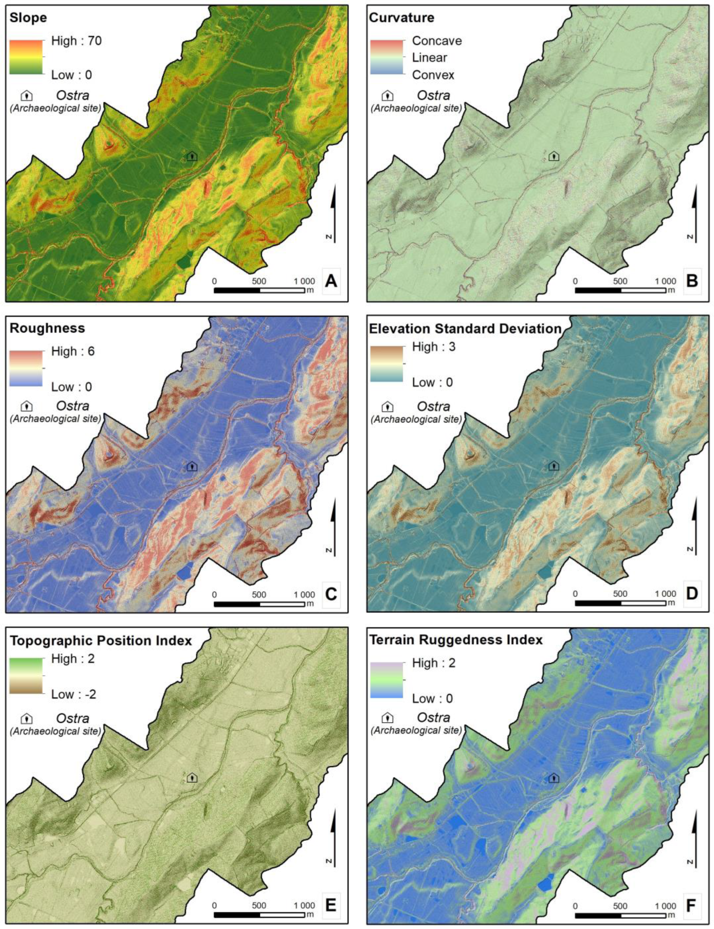
The quantitative characterization of the topography, aimed at identifying the fluvial terraces, was carried out considering the geometric properties of the specific landforms being detected. As a result, 7 morphometric parameters, both primary and secondary [
31], were selected. Namely, the computed morphometric parameters are slope (S), curvature (C), roughness (R), elevation standard deviation (ESD), topographic position index (TPI), terrain ruggedness index (TRI), and geomorphons. The primary parameters, which consider a moving window with respect to the central cell in the computation, comprise local parameters both of geometric (slope and curvature) and statistical types (roughness and elevation standard deviation). Between the secondary parameters, both indexes (the topographic position index and terrain ruggedness index) and objects (geomorphons) have been considered. The first was intended as a combination of primary parameters [
32], while the second was conceived as an elementary unit expressing geometric terrain types [
33]. These parameters have been selected with the purpose of remotely supporting the identification of terraces and evaluating their specific statistics in each terrace order. The considered morphometric parameters consist of 6 of continuous type (slope, curvature, roughness, elevation standard deviation, topographic position index, and terrain ruggedness index) and 1 of categorical type (geomorphons).
S (
Figure 4A) has been calculated by exploiting the algorithm running in the Spatial Analyst tool of the ArcGIS software, which considers the parameter as the first derivative of the elevation surface or the maximum change in elevation on a cell-by-cell basis [
34]. This geometric parameter has been considered, as it is considered to be a basic variable for defining the specific signature of several geomorphic processes [
35].
C (
Figure 4B) was calculated by combining the planform and the profile values in order to estimate the magnitude of the concavity and convexity of the land surface and to describe the general shape of the slopes [
36]. Curvature was computed by exploiting the algorithm running in the Spatial Analyst tool of the ArcGIS software.
R (
Figure 4C) is a local-statistical parameter and was computed by considering the largest inter-cell absolute difference of a focal cell and its surroundings [
14,
37], defined as a 3 × 3 cell moving window. The R values were computed using the focal statistics approach in the Spatial Analyst tool of the ArcGIS software and the Raster calculator tool.
ESD (
Figure 4D) is a parameter of the local-statistic type and was computed by performing a neighborhood operation using a 3 × 3 moving window, wherein the output value for each cell represents the standard deviation value within the considered window. ESD is a measure of the amount of variation in height within the selected area, with values close to zero indicating flat zones. The ESD values were computed using the focal statistics approach in the Spatial Analyst tool of the ArcGIS software.
TPI (
Figure 4E) measures the difference between the elevation at a central point with respect to the average elevation of its neighborhood, and it is used to describe the relative position of the cells of the DTM with respect to the surrounding area [
38,
39]. This parameter is highly scale-dependent and enables one quantitatively express the morphology of the area being considered. In this study, TPI values were computed by considering an area corresponding to the 3 × 3 windows adopted in the calculation of other morphometric parameters. TPI was calculated with the specific GDAL tool available in the QGIS software.
TRI (
Figure 4F) represents a measurement of the topographic heterogeneity quantifying the mean value of the absolute difference in elevation between a focal cell and its surroundings [
40]. In our study, it is defined in in a 3 × 3 cell window. TRI was calculated with the specific GDAL tool available in the QGIS software.
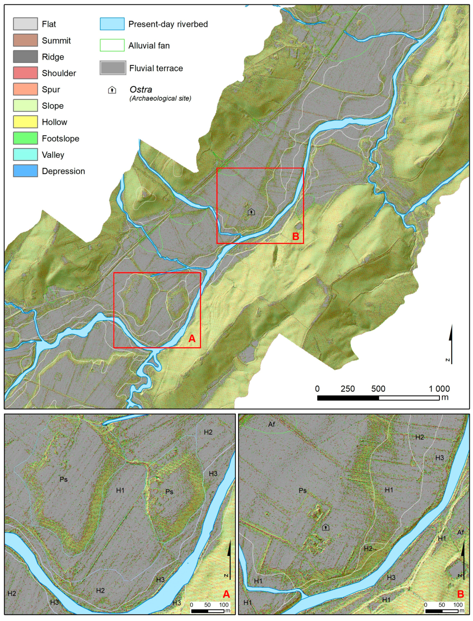
Geomorphons (
Figure 5) are an object-based parameter which identifies geomorphological types based on pattern recognition rather than differential geometry. This parameter consists of 10 classes which classify the terrain in terms of the following features: depression (or pit), flat, footslope, hollow, ridge, shoulder, slope, spur, summit (or peak), and valley [
33]. The geomorphon parameter was calculated using the specific GRASS tool available in the QGIS software. Geomorphons were computed considering several combinations of input information, among which the best-performing example considered an outer search radius equal to 3, an inner search radius of 0, and a flatness threshold equal to 3°.
4. Results
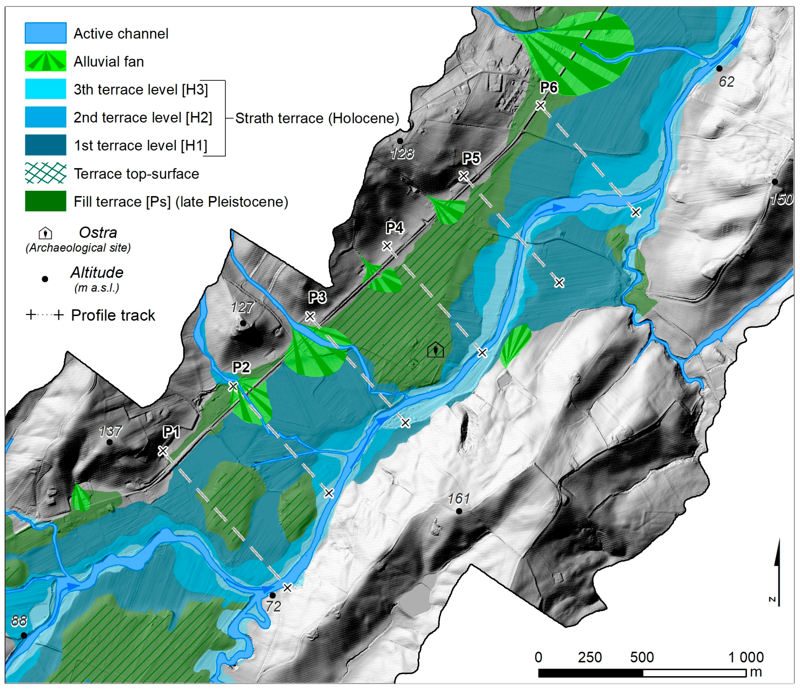
The field survey allowed us to distinguish the main terrace generation (
Figure 3), corresponding to the late Pleistocene fill terrace, thanks to the good preservation of the planar geometry of the terrace top–surface, which hangs at a mean of 12–16 m above the present thalweg, and the large presence, above and immediately below of this thalweg, of well-rounded fluvial cobbles of different dimensions, taken as markers of the late Pleistocene gravel deposits ([
16] and references therein). The presence of gravel above the terrace surface seems to diminish starting at the higher terrace level and continuing to the lower ones. Despite the good preservation of the original geometry of the late Pleistocene terrace top–surface, the inner and external edges of the main terrace have not been successfully recognized in the field because of the profound remodeling caused by agricultural practices, hydraulic works, urbanization, and the overall very low altitudinal differences between the single terrace features. Furthermore, the inner terrace edge, corresponding to the inner margin of the present valley floor, is often crossed by a main road, is fringed by a shallow colluvial cover, and, at the main tributary streams, is at places hidden by wide alluvial fan bodies (
Figure 3). The latter have been reported in the geomorphological scheme, and their limits have been mapped using aerial photo interpretation based on the different colors and textures shown by different landforms [
41]. The limits between the main, late Pleistocene fill terrace reported in the present geological map and the Holocene terraces have been checked and adjusted where possible thanks to the presence of a remolded scarp that, at places, preserved the original landform geometry (
Figure 3b). On the contrary, as expected, the distinction between different minor terrace steps starting from those of the late Pleistocene (hanging at heights from few meters up to about 10 m from the present thalweg) has not been possible due to the apparent absence in the field of recognizable landforms and deposit outcrops. In addition, field survey allows for the recognition that the active river channel is characterized by bedrock typology and, at places, is covered by a thin alluvial cover represented by shallow gravel bars. The bedrock incising tendency of the active river channel is also testified to by the presence of 2–3 m high, sub-vertical active river banks fringing the active channel with a relative spatial continuity.
To support the field survey findings, a visual inspection of the spatial distribution of the selected morphometric parameters was carried out (
Figure 4 and
Figure 5). This visual inspection was conducted by cross-checking the outputs, specifically symbolized to optimize the thresholds between significant values, of the LSQ analysis.
In the S output, the contrast between the floodplain and the slope sector is evident as well as the location of the present active channels (
Figure 4A). Major S values are found in correspondence with the present-day riverbeds and along slopes that are mainly occupied by landslides and alluvial fans. Furthermore, in the defined floodplain, the geometric delineation between the late Pleistocene and Holocene fluvial terraces is evident, as the former are surrounded by noticeable slope breaks which contoured the terrace top–surface. Likewise in the R, ESD, and TRI outputs (
Figure 4C,D,F) where these same distinctions are detectable, with differences are mainly due to the range of values computed and the graduated color scale employed. The C and TPI outputs (
Figure 4B,E), conversely, do not supply an effective visual support for terrace identification, as the wide value range is opposed by a limited variance of around zero. Finally, the 10 classes of geomorphons (
Figure 5) allow for a more detailed description of the local morphology and relative changes, especially when a 1 m resolution DTM is employed, as is the case in this study site; however, they require a large-scale interpretation and an overall generalization in order to be functional for fluvial terrace delimitation (
Figure 5A,B). The floodplain, clearly distinguishable from the slope sectors, is dominated by the flat class interspersed with alternating geometries (i.e., hollow, footslope, and spur) which describe the slope breaks and corresponding fluvial terrace limit.
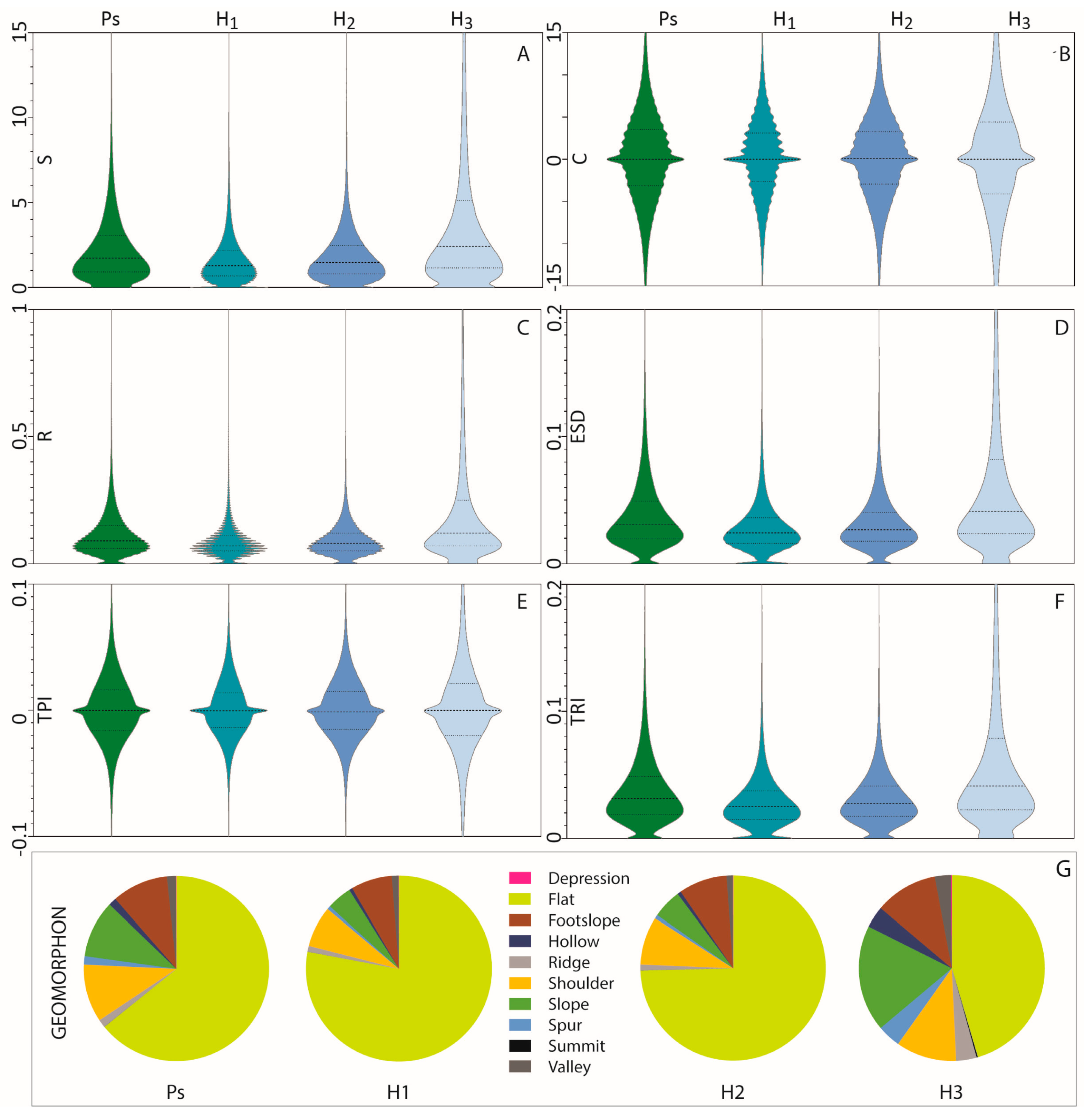
The computed S values show a value range from 0° to 69.78° (
Figure 4A,
Table 1) with a mean value of about 7°, median value of about 5°, and a third quartile of about 10°. If only terraced deposits are considered, then the mean value drops by about to 2° with 87% of the values less being than 5°, and 94% of the values being less than 10°. Differences in S-value distribution between the Ps terraces and H terraces are slightly delineable, as the former have a mean value of 2.53°, while the latter present a mean value of 3.50°. More detectable, especially in relation to the small range of values, are the distinctions that fit out in the S values of the three Holocene terrace levels; H1 shows a lower median value equal to 1.30° in comparison with the median value of the H3 level, which is equal to 2.43° (
Figure 6A).
The C values present a mean value of 0.13 × 10
−2 m and a median value of about 0.00 × 10
−2 m, with a third quartile of 4.99 × 10
−2 m (
Figure 4B,
Table 1). Taking into account the terraced deposits, the mean value is 0.15 × 10
−2 m for the Ps terraces and 0.33 × 10
−2 m for the H ones. The zones with positive C values represent about 50% of the total terraced deposits, while the flat zones represent 6%, and the zones with negative C values represent about 44%. Despite the high range in values, 94% of the values are in the range from −15 × 10
−2 m to 15 × 10
−2 m (
Figure 6B). C value distribution does not considerably differ between Ps and H terraces; in fact, respectively, the median values are 0.00 and 0.03 × 10
−2 m, the mean values are 0.15 and 0.33 × 10
−2 m, and the third quartile is 3.54 and 3.73× 10
−2 m. Even the contrast between the three H terrace levels is marginally marked, except for the H3 level, which presents distinct values for the first and third quartiles, respectively, equal to −4.11 and 4.43 × 10
−2 m.
The R morphometric parameter exhibits values ranging from 0 m to 5.68 m (
Figure 4C,
Table 1) with a mean value of 0.33 m, a median value of 0.23 m, and a third quartile of about 0.47 m. Considering terraced deposits, the mean value is 0.12 m, with 91% of the values being less than 0.23 m and 97% of the values being less than 0.47 m (
Figure 6C). As for S values, differences in value distribution between Ps terraces and H terraces are hardly delineable, as all parameters are very close in value, but the distinction between the three Holocene terraces appears to be identifiable. Though H1 and H2 are distinguished by limited differences in value distribution, H3 presents a different distribution, with a median value of 0.12 m and a third quartile equal to 0.25 m.
ESD values range between 0.00 and 2.31 m (
Figure 4D,
Table 1) with a median value of 0.08 m and with first and third quartiles, respectively, of 0.03 and 0.15 m. A total of 97% of the terraced deposits show values less than 0.15 m (
Figure 6D). Ps statistics do not differ from H values, but for this parameter some differences are notable between the three H levels and, in particular, in the H3 level.
TPI morphometric index offers values which are more difficult to interpret both through visual inspection and numerical interpretation. Values range between −2.58 m and 2.78 m (
Figure 4E,
Table 1), but the descriptive statistics show an equivalent distribution, as 91% of the total study area presents values ranging between −0.1 and 0.1 m, and this percentage rises to 98% if only terraced deposits are considered. The small range of values does not allow for the detection of significant differences, only the H3 level stands out slightly, as already noted in the other morphometric parameters, with the first and third quartiles, respectively, being equal to −0.02 and 0.02 m (
Figure 6E).
The computed TRI values show a value range from 0 to 2.78 m (
Figure 4F,
Table 1) with a mean value of about 0.1 m, a median value of 0.07 m, and a third quartile of about 0.15 m. If only terraced deposits are considered, then the mean value drops to about 0.04 m, with 90% of the values being less than 0.07 m, and 97% of the values being less than 0.15 m. Differences in the TRI value distribution between Ps terraces and H terraces are, as shown by the above-mentioned morphometric parameters, slightly delineable, as the descriptive statistic values are close to be equal. Appreciable are, instead, the distinctions that fit out between the H3 terrace level and the other two H1 and H2 levels (
Figure 6F). In particular, H3 shows high values for the median and third quartile equal to 0.04 and 0.08 m, respectively.
Geomorphon outputs are of categorical type, and they consequently have been analyzed by means of visual inspection (
Figure 5) and with consideration for the general distribution of the 10 classes within the alluvial terraces (
Figure 6G,
Table 2). The study area feature types are predominantly slope (38%) and flat (32%), followed by shoulder (7%), spur (7%), footslope (6%), hollow (6%), and then the remaining classes. In the alluvial terraces, the dominant feature is flat, with a percentage of 64% for Ps terraces and 72% for H terraces (respectively 78%, 75%, and 45%). Next in line are footslope and shoulder with percentages of 10% in Ps terraces and 8% in H terraces. Slope type represents a percentage of 10% in the Ps terraces and 7% in H terraces. Other features are irrelevant with percentages less than 2% both for Ps and H terraces. Considering the distribution characterizing the three H levels, notably the H3 distinction with flat features less than 50% and a relatively high percentage of slope, footslope, and shoulder types as well as a generalized percentage higher that both Ps and other H terraces.
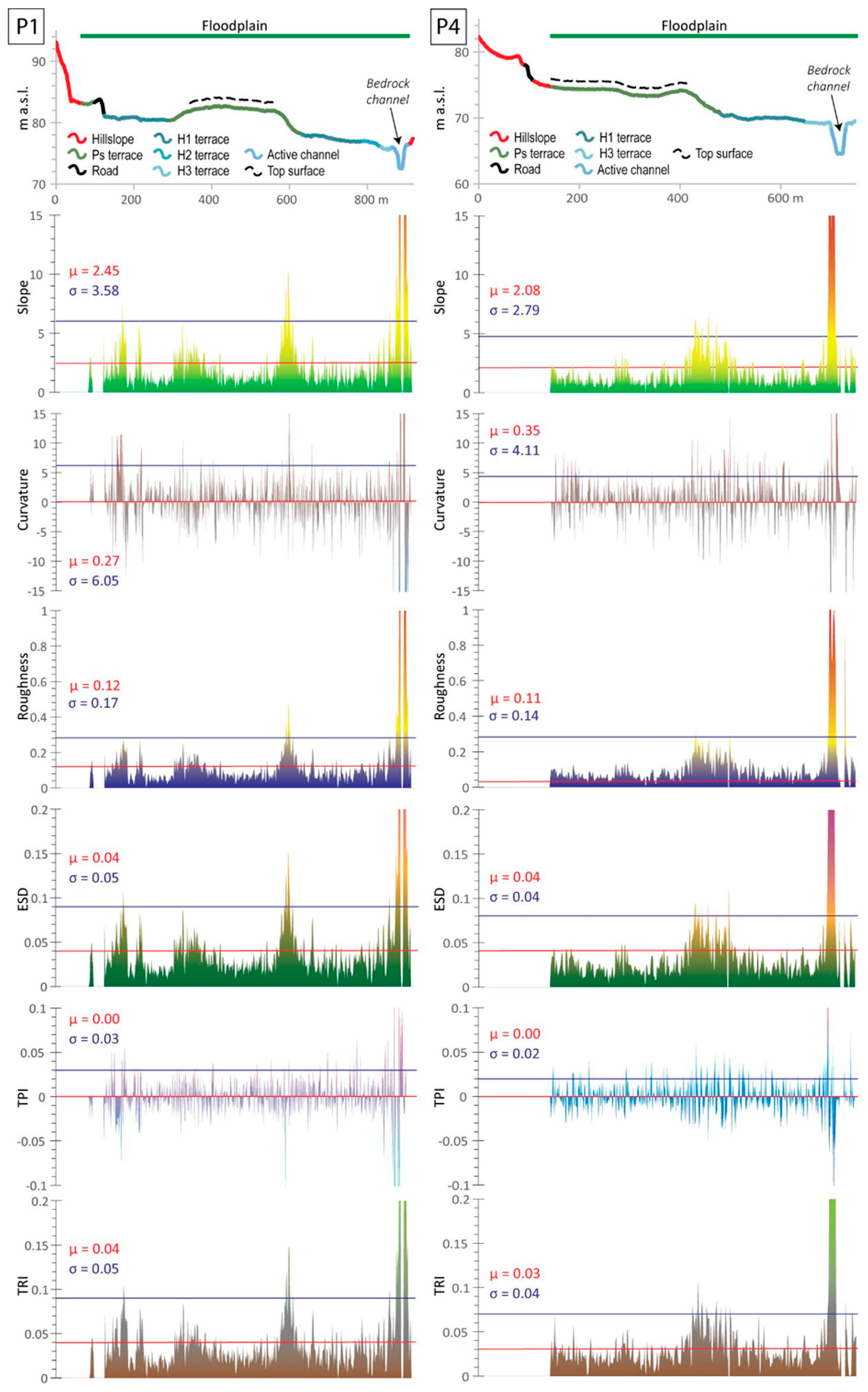
The spatial distribution of morphometric continuous parameters has been also compared, considering their trends (
Figure 7) along with selected altimetric profiles (P1–P6 in
Figure 8). S, R, ESD, and TRI show observable peaks, denoting evident changes in values, which are supportive to locating the boundaries between different terrace levels as well as to top surface identification. Meanwhile, C and TPI exhibit fluctuating trends which are not interpretable for terrace delimitation. In
Figure 7, by way of example, the trends along P1 and P4 are shown. In both, S, R, ESD, and TRI display analogous trends with peak values, those higher than the mean corresponding with terrace limits and low steady values, those lower than the mean, in correspondence with the terrace top–surface. All of the parameters show a noticeable peak at the first flex point above the talweg, potentially marking the height of the channel bankfull. In particular, the C parameter shows a rapid switch from negative to positive values, confirming the occurrence of a flex point at the external margin of the floodplain, above the present active channel.
5. Discussion
Despite previous studies and the efforts made in the field, the individuation of some terrace features and the assessment of their spatial distribution and continuity remained elusive, therefore, LSQ analysis has been supportive to obtaining more detailed identifications and precise mapping.
Field surveys have proven to be of basic relevance in identifying the terrace typologies (fill and strath) for both Ps and H levels. A main terrace of fill typology (Ps on
Figure 2B) and three different discontinuous levels of strath terraces (H1, H2, and H3 on
Figure 2B) compose the fluvial terraces staircase in the analyzed sector of the Adriatic side of the northern Marche Apennines, confirming the model proposed [
16] for the arrangement of the main floodplains in the study region (
Figure 7 and
Figure 8). The highest and most continuous fill terrace, corresponding to the T3 terrace generation [
20], formed during the late Pleistocene under cold, full-glacial conditions. Gravels and sands of braided-type river pattern compose the terrace deposits, whose sedimentation ended at about 14 ka (see the scheme of valley development reported in [
18], which is valid for the mid and lowermost section of the river valleys draining the Adriatic side of the Marche Apennines). The main late-Pleistocene fill terrace shows a sub-planar terrace top–surface, well-continued along the valley and slightly dipping toward the main channel at the valley bottom and hanging at heights between 10 and 16 m above the present thalweg. The terrace surface at places results as being remolded by tributary streams’ entrenchment and human activities. Starting from this terrace surface, at lower heights between 3–4 and 9–10 m above the preset thalweg, a series of discontinuous terrace steps can be found due to episodic overbank sedimentation during a general entrenchment phase [
42], changing river regimes coupled with lateral river migrations [
43], and/or in-grown meanders [
20,
24]. Therefore, considering the thin depositional cover never exceeding 2–3 m in thickness [
20,
23,
24], these terrace levels can reasonably be interpreted as strath terraces generated in short episodes of river stationarity. Accordingly, minor filling stages account for thin gravel and sand deposition during a general post-glacial downcutting phase, the latter characterizing the entirety of the Holocene fluvial morphodynamics at the inner portion of the river basins in the study region. Extreme flooding events, such as the one which occurred on 16 September 2022, to cite the most recent, have reached the heights of the lowest terrace levels. Therefore, at places, it is somewhat difficult to distinguish these younger and lower levels from the flooding area. The latter is due to the plain inundation by either the main watercourse or tributary streams along their lowermost sectors crossing the floodplain.
In this research, no chronological investigations have been done, and therefore the chronology of the terrace generations here described has been extrapolated by adopting mere extra-valley correlation criteria which have already been adopted and accepted for the study region [
8,
18,
19,
20,
24] based on similar terrace generations located at the same position along valley sides and floodplains. Nonetheless, the position of the ancient Roman village of Ostra, lying at the margin of the late Pleistocene fill terrace top–surface, supports the adopted relative chronology, interpreting the three strath terrace levels, according to [
28,
29,
30], as early Holocene (10–8.0 ka BP) and late Holocene (ca. 3–2 ka BP and VI–VII century AD) in age, from the higher to the lower one, respectively. Obviously, the lack of absolute chronological constraints in the specific study site provides a wide margin of uncertainty with regard to the hypothesized terrace chronology, and, considering the climate and tectonic relevance of the terrace record here described, the geomorphological results of this work should be taken as stimulus for further targeted research.
The computation and the assessment (both visual and objective) of the selected morphometric parameters have indeed allowed for the refinement of terrace features’ identification, completing the conventional geomorphological field surveys and remote imagery interpretations. In particular, the LSQ analysis allows for evaluation of the general along-valley continuity of the Ps surface, refinement of the identification of the terrace top–surfaces, as well as relocation of the Holocene terrace boundaries (H1, H2 and H3), also identifying their along-valley continuity.
The morphometric parameters S, R, ESD, TRI, and geomorphons (
Figure 4A,C,D,F and
Figure 5) have proven to be effective in supporting the visual interpretation of the investigated fluvial landforms. Conversely, C and TPI were demonstrated to be unreliable in highlighting the limits of fluvial terrace sequence, even if they did contribute to delineating the overall morphology of the considered sector (
Figure 4B,E). Corresponding consideration also emerged from the quantitative evaluation of the descriptive statistics of the parameter values (
Table 1 and
Table 2 and
Figure 6). It is noticeable that these assessments can support the distinction between the slope sectors and the fluvial terraced deposits as well as the detection of the three Holocene terrace levels. Among these, the characterization of the most recent one (H3) turned out to be particularly evident, as it shows distinctive values for most parameters (
Table 1 and
Table 2).
The interpretation of parameters’ values along some profiles and their comparison with the high-detail altimetry derived from LiDAR (
Figure 7) allowed for the inner margin of the higher terrace generation to be clearly distinguished, and thus the boundary between the hillslope and floodplain. Along the single profiles, both principal and minor terrace scarps can be identified, thus allowing for a good distinction between the single terrace generations. Moreover, marked by a peak in the C parameter, the channel bankfull can be identified, resulting in the first flex point above the thalweg and the external, channel-wards margin of the floodplain.
The main limitations of the proposed approach are the impossibility of estimating the terrace deposits belonging to the ancient fill terrace generation, and intrinsic difficulties in identifying some small terrace remnants belonging to the youngest strath generations due to the very small altimetric differences between some of them and the presence of some DTM artifacts.
6. Conclusions
In this work a combined geomorphological approach based on a field survey and land-surface quantitative (LSQ) analysis has been applied for better identification and the detailed mapping of fluvial terraces along low-relief floodplains. The late Pleistocene–Holocene fluvial terrace staircase along a segment in the mid-Misa River valley has been taken as an example of the floodplains developing along the Adriatic side of the Marche Apennines. Here, the combination of fieldwork with the assessment of some morphometric parameters (S, C, ESD, R, TPI, TRI, and geomorphons) derived from a high-resolution DTM, were demonstrated to enhance the identification and mapping of fluvial terraces. Thus, this combined approach allowed for distinguishing and mapping in detail the main terrace generation characterized by the fill typology, the well-developed and continuous terrace surface, and the remodeled, ca. 3 m-high, low-angle terrace scarp that separates the terrace top–surface from the lower and younger terrace generations. These latter are of strath typology, formed during the Holocene, rarely display a well-developed surface, and are discontinuous, though the first Holocene terrace is the most developed. The main terrace was formed during the late Pleistocene under full-glacial, cold conditions, whereas the younger ones were formed at periods of channel stationarity during the general post-glacial downcutting phase.
From a methodological point of view, the field surveys were revealed to be precious for distinguishing the terrace typologies and verifying the results from the quantitative remote analyses. These latter were helpful for distinguishing the different Holocene terrace levels and assessing their along-valley distribution, as well as for objectively identifying and mapping the top–surface of the main fill terrace generation.
The proposed approach, which includes both field surveys and quantitative analysis based on a high-resolution DTM, led to distinguishing the late Pleistocene–Holocene fluvial terrace staircase, thus taking advantage of the quantitative characterization of the geometric properties of these specific fluvial landforms.
The presented approach can potentially be adopted as a preliminary investigation for remote study areas, where field surveys can more-or-less be conducted. Moreover, the early distinction between fluvial terrace features (i.e., top–surface and main scarps) is useful for a preliminary selection of sampling areas, where dating and additional analysis can be conducted for the chronological and sedimentological characterization of the fluvial deposits. Finally, the proposed approach can be reliable for detailing previous geomorphological maps as well as their first fulfillment.


