


A Comparison of Semilandmarking Approaches in the Analysis of Size and Shape
Abstract
:Simple Summary
Abstract
1. Introduction
2. Materials and Methods
2.1. Samples
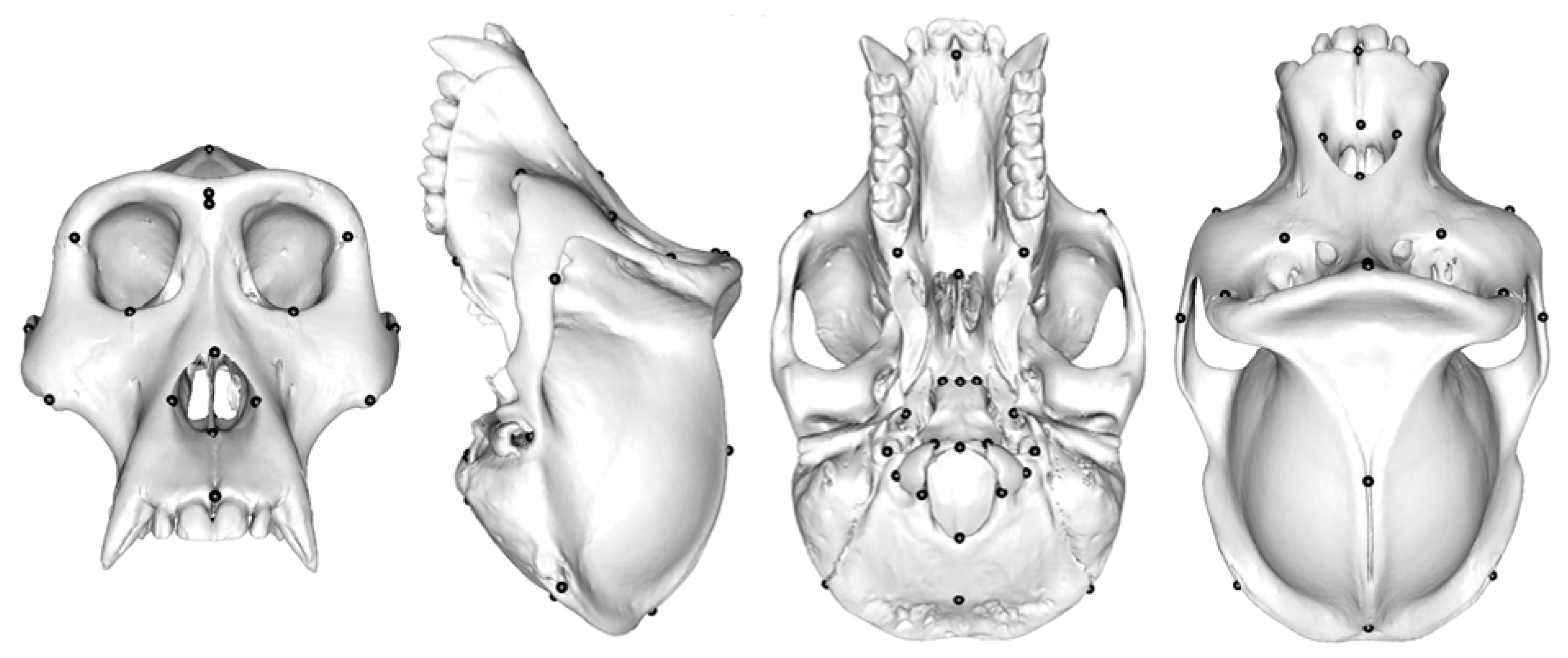
Ape Crania
2.2. Methods
2.2.1. Three Semilandmarking Approaches
Generation of the Template
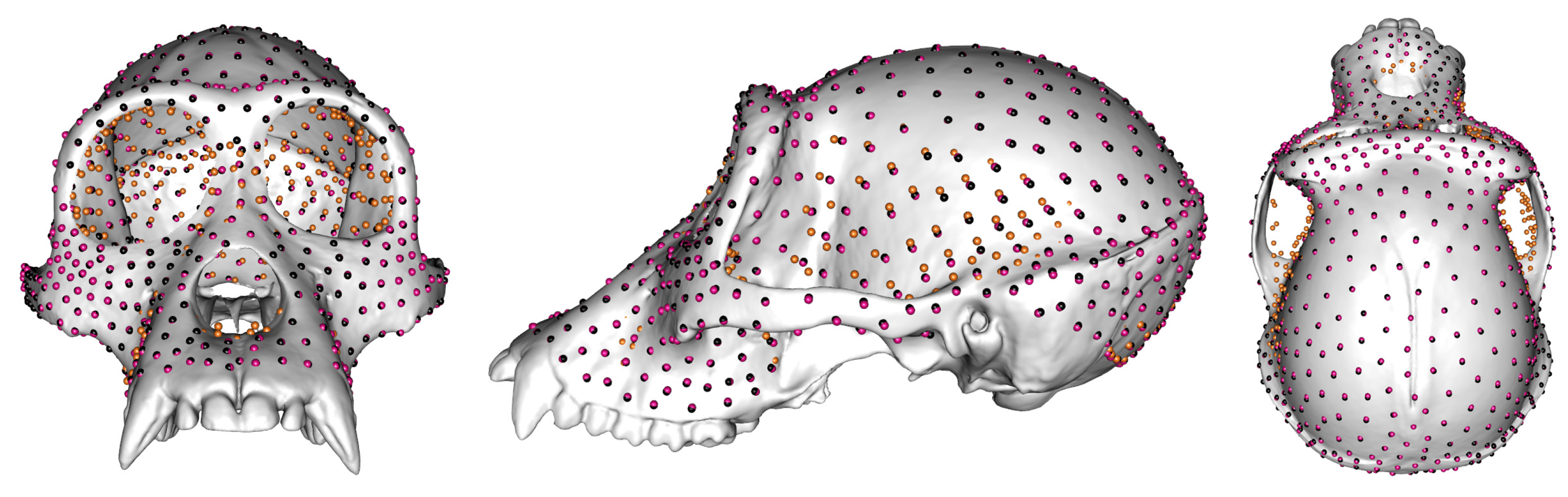
Semilandmarking Approaches
- (a)
- Sliding TPS
- (b)
- Rigid registration
- (c)
- Non-rigid registration
2.2.2. Comparison of Three Semilandmarking Approaches
The Locations of Semilandmarks
Comparisons of Mean Landmark and Semilandmark Configurations
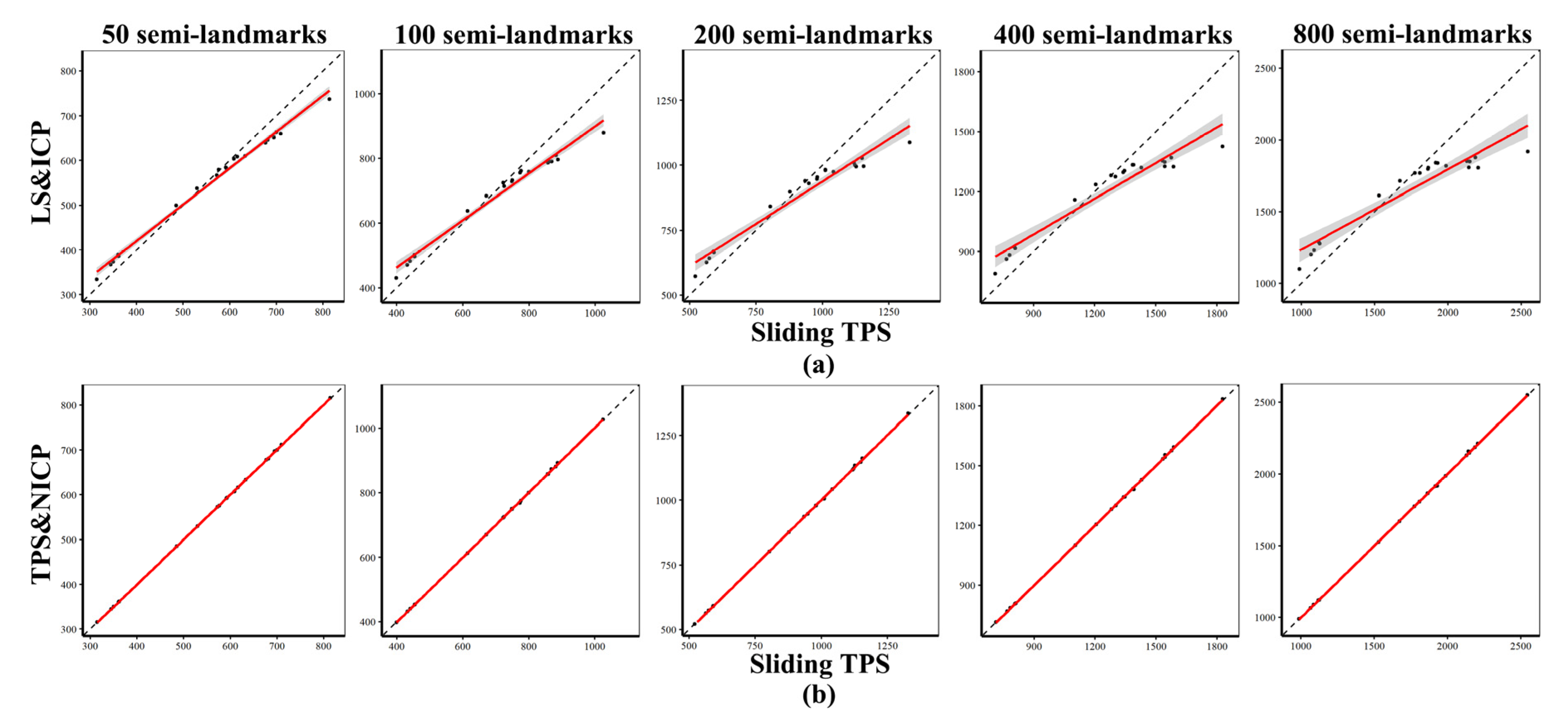
Procrustes Distances among Specimens Obtained Using Different Semilandmarking Approaches and Densities
- (a)
- The effect of different semilandmarking approaches
- (b)
- The effect of different densities of semilandmarks
PCA and Allometry
3. Results
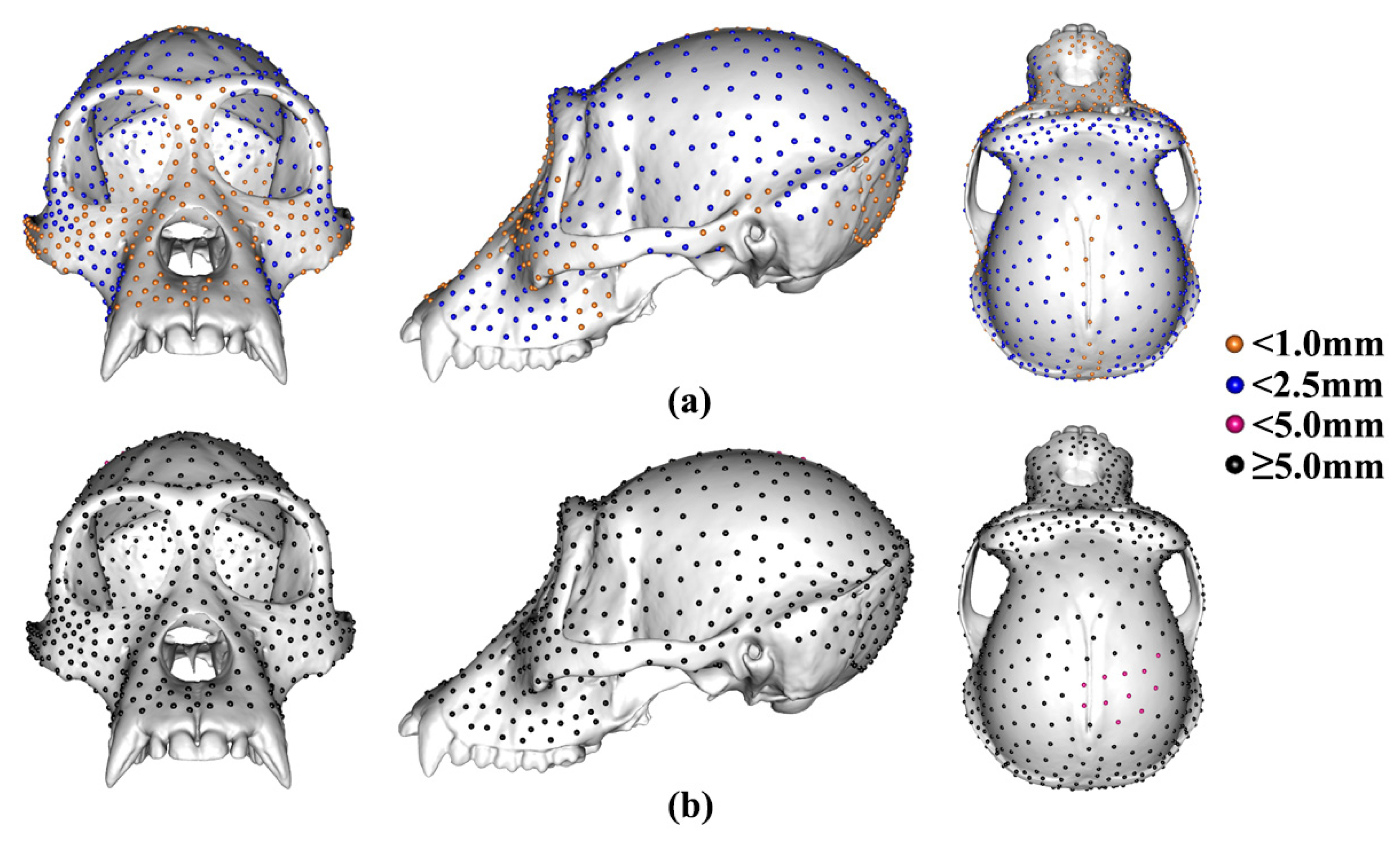
3.1. The Locations of Semilandmarks
3.2. Differences among Mean Landmark and Semilandmark Locations
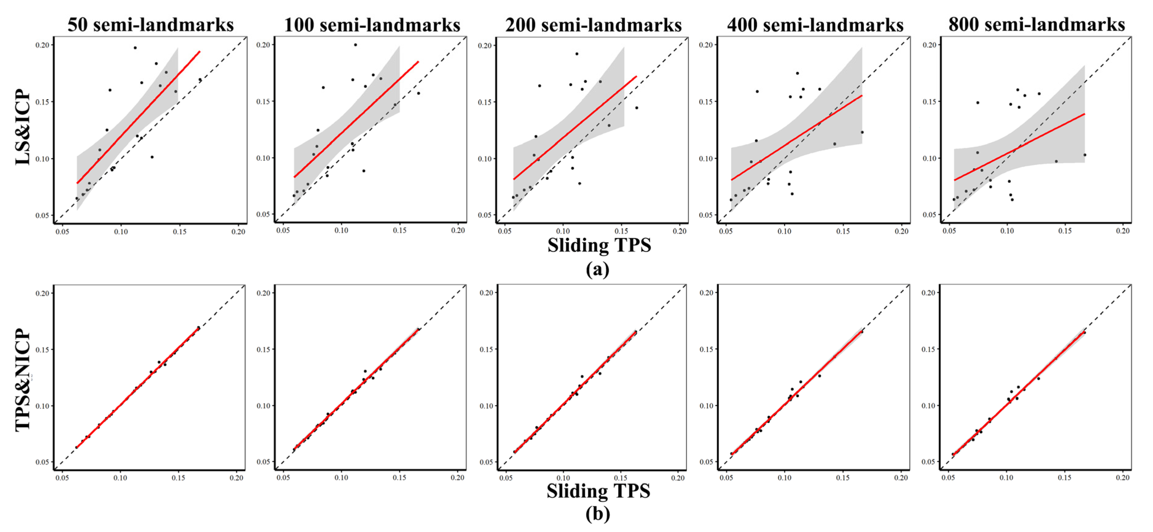
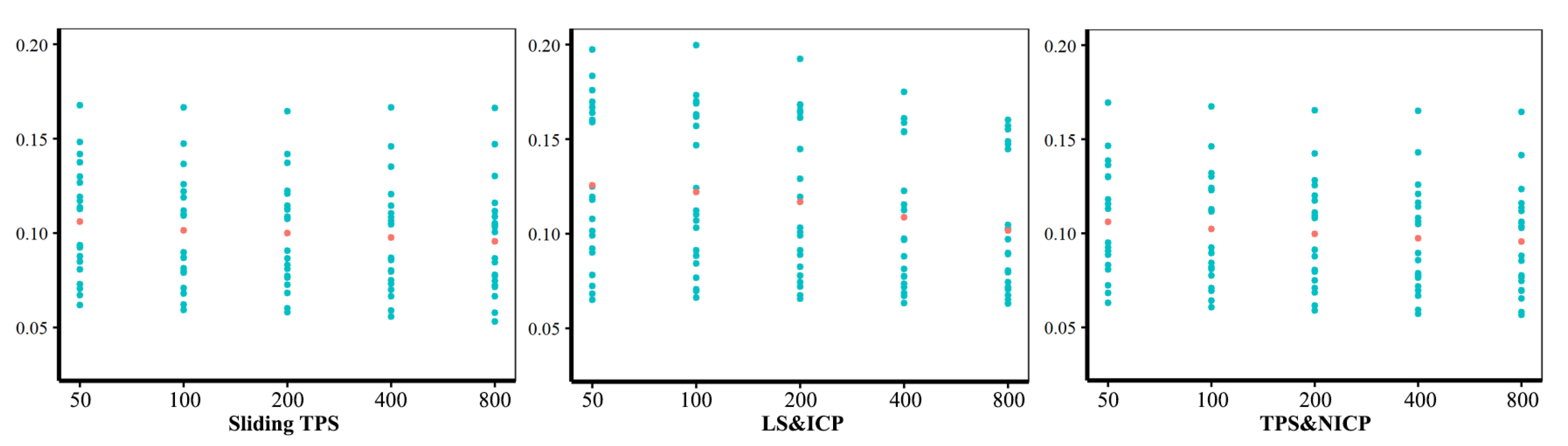
3.3. Comparison of Centroid Sizes and Procrustes Distance Matrices
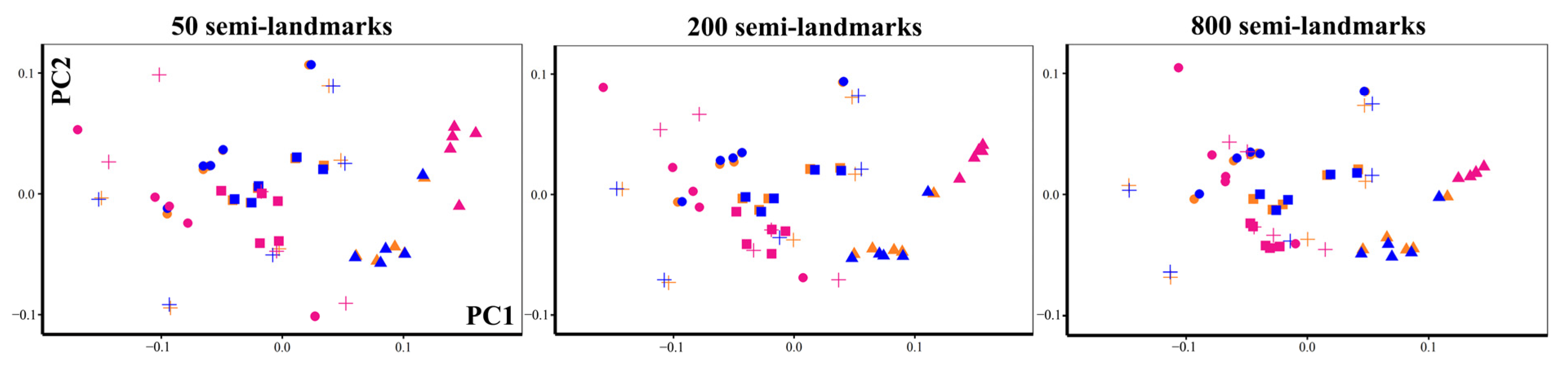
3.4. PCA and Allometry
4. Discussion
4.1. Significance and Implications of Findings
4.2. Limitations and Future Work
5. Conclusions
Supplementary Materials
Author Contributions
Funding
Institutional Review Board Statement
Informed Consent Statement
Data Availability Statement
Acknowledgments
Conflicts of Interest
References
- O’Higgins, P. The study of morphological variation in the hominid fossil record: Biology, landmarks and geometry. J. Anat. 2000, 197, 103–120. [Google Scholar] [CrossRef]
- Adams, D.; Rohlf, J.; Slice, D. Geometric morphometrics: Ten years of progress following the ‘revolution’. Ital. J. Zool. 2004, 71, 5–16. [Google Scholar] [CrossRef] [Green Version]
- Viscosi, V.; Cardini, A. Leaf morphology, taxonomy and geometric morphometrics: A simplified protocol for beginners. PLoS ONE 2011, 6, e25630. [Google Scholar] [CrossRef] [PubMed] [Green Version]
- Mitteroecker, P.; Gunz, P. Advances in geometric morphometrics. Evol. Biol. 2009, 36, 235–247. [Google Scholar] [CrossRef] [Green Version]
- Mitteroecker, P.; Schaefer, K. Thirty years of geometric morphometrics: Achievements, challenges, and the ongoing quest for biological meaningfulness. Am. J. Biol. Anthropol. 2022, 178, 181–210. [Google Scholar] [CrossRef]
- Marshall, A.F.; Bardua, C.; Gower, D.J.; Wilkinson, M.; Sherratt, E.; Goswami, A. High-density three-dimensional morphometric analyses support conserved static (intraspecific) modularity in caecilian (Amphibia: Gymnophiona) crania. Biol. J. Linn. Soc. 2019, 126, 721–742. [Google Scholar] [CrossRef] [Green Version]
- Blanz, V.; Vetter, T. A morphable model for the synthesis of 3D faces. In Proceedings of the 26th Annual Conference on Computer Graphics and Interactive Techniques, Los Angeles, CA, USA, 1 July 1999; pp. 187–194. [Google Scholar]
- Bookstein, F.L. Landmark methods for forms without landmarks: Morphometrics of group differences in outline shape. Med. Image Anal. 1997, 1, 225–243. [Google Scholar] [CrossRef]
- Oxnard, C.; O’Higgins, P. Biology clearly needs morphometrics. Does morphometrics need biology? Biol. Theory 2009, 4, 84–97. [Google Scholar] [CrossRef]
- Rolfe, S.; Davis, C.; Maga, A.M. Comparing semi-landmarking approaches for analyzing three-dimensional cranial morphology. Am. J. Phys. Anthropol. 2021, 175, 227–237. [Google Scholar] [CrossRef] [PubMed]
- Gunz, P.; Mitteroecker, P.; Bookstein, F.L. Semilandmarks in three dimensions. In Modern Morphometrics in Physical Anthropology; Springer: Berlin, Germany, 2005; pp. 73–98. [Google Scholar]
- Perez, S.I.; Bernal, V.; Gonzalez, P.N. Differences between sliding semi-landmark methods in geometric morphometrics, with an application to human craniofacial and dental variation. J. Anat. 2006, 208, 769–784. [Google Scholar] [CrossRef]
- Gunz, P.; Mitteroecker, P. Semilandmarks: A method for quantifying curves and surfaces. Hystrix Ital. J. Mammal. 2013, 24, 103–109. [Google Scholar]
- Chui, H.; Rangarajan, A. A new point matching algorithm for non-rigid registration. Comput. Vis. Image Underst. 2003, 89, 114–141. [Google Scholar] [CrossRef]
- Mydlová, M.; Dupej, J.; Koudelová, J.; Velemínská, J. Sexual dimorphism of facial appearance in ageing human adults: A cross-sectional study. Forensic Sci. Int. 2015, 257, 519. e511–519. e519. [Google Scholar] [CrossRef]
- Musilová, B.; Dupej, J.; Velemínská, J.; Chaumoitre, K.; Bruzek, J. Exocranial surfaces for sex assessment of the human cranium. Forensic Sci. Int. 2016, 269, 70–77. [Google Scholar] [CrossRef]
- Amberg, B.; Romdhani, S.; Vetter, T. Optimal step nonrigid ICP algorithms for surface registration. In Proceedings of the IEEE Conference on Computer Vision and Pattern Recognition (CVPR’07), Minneapolis, MN, USA, 17–22 June 2007; pp. 1–8. [Google Scholar]
- Booth, J.; Roussos, A.; Ponniah, A.; Dunaway, D.; Zafeiriou, S. Large scale 3D morphable models. Int. J. Comput. Vis. 2018, 126, 233–254. [Google Scholar] [CrossRef] [Green Version]
- Shui, W.; Zhou, M.; Maddock, S.; Ji, Y.; Deng, Q.; Li, K.; Fan, Y.; Li, Y.; Wu, X.J. A computerized craniofacial reconstruction method for an unidentified skull based on statistical shape models. Multimed. Tools Appl. 2020, 79, 25589–25611. [Google Scholar] [CrossRef]
- White, J.D.; Ortega-Castrillón, A.; Matthews, H.; Zaidi, A.A.; Ekrami, O.; Snyders, J.; Fan, Y.; Penington, T.; Van Dongen, S.; Shriver, M.D. MeshMonk: Open-source large-scale intensive 3D phenotyping. Sci. Rep. 2019, 9, 6085. [Google Scholar] [CrossRef] [Green Version]
- Dai, H.; Pears, N.; Smith, W.; Duncan, C. Statistical Modeling of Craniofacial Shape and Texture. Int. J. Comput. Vis. 2020, 128, 547–571. [Google Scholar] [CrossRef] [Green Version]
- Van Kaick, O.; Zhang, H.; Hamarneh, G.; Cohen-Or, D. A survey on shape correspondence. Comput. Graph. Forum 2011, 30, 1681–1707. [Google Scholar] [CrossRef] [Green Version]
- Besl, P.J.; McKay, N.D. A method for registration of 3-D shapes. IEEE Trans. Pattern Anal. Mach. Intell. 1992, 14, 239–256. [Google Scholar] [CrossRef] [Green Version]
- Rusinkiewicz, S.; Levoy, M. Efficient variants of the ICP algorithm. In Proceedings of the Third IEEE International Conference on 3-D Digital Imaging and Modeling, Quebec City, QC, Canada, 28 May–1 June 2001; pp. 145–152. [Google Scholar]
- Pomidor, B.J.; Makedonska, J.; Slice, D.E. A landmark-free method for three-dimensional shape analysis. PLoS ONE 2016, 11, e0150368. [Google Scholar] [CrossRef]
- Boyer, D.M.; Puente, J.; Gladman, J.T.; Glynn, C.; Mukherjee, S.; Yapuncich, G.S.; Daubechies, I. A new fully automated approach for aligning and comparing shapes. Anat. Rec. 2015, 298, 249–276. [Google Scholar] [CrossRef] [PubMed] [Green Version]
- Vitek, N.S.; Manz, C.L.; Gao, T.; Bloch, J.I.; Strait, S.G.; Boyer, D.M. Semi-supervised determination of pseudocryptic morphotypes using observer-free characterizations of anatomical alignment and shape. Ecol. Evol. 2017, 7, 5041–5055. [Google Scholar] [CrossRef]
- Gao, T.; Yapuncich, G.S.; Daubechies, I.; Mukherjee, S.; Boyer, D.M. Development and assessment of fully automated and globally transitive geometric morphometric methods, with application to a biological comparative dataset with high interspecific variation. Anat. Rec. 2018, 301, 636–658. [Google Scholar] [CrossRef] [PubMed] [Green Version]
- Wang, S.; Wang, Y.; Jin, M.; Gu, X.D.; Samaras, D. Conformal geometry and its applications on 3D shape matching, recognition, and stitching. IEEE Trans. Pattern Anal. Mach. Intell. 2007, 29, 1209–1220. [Google Scholar] [CrossRef] [Green Version]
- Gu, X.; Wang, Y.; Chan, T.F.; Thompson, P.M.; Yau, S.-T. Genus zero surface conformal mapping and its application to brain surface mapping. IEEE Trans. Med. Imaging 2004, 23, 949–958. [Google Scholar] [CrossRef]
- Boyer, D.M.; Lipman, Y.; Clair, E.S.; Puente, J.; Patel, B.A.; Funkhouser, T.; Jernvall, J.; Daubechies, I. Algorithms to automatically quantify the geometric similarity of anatomical surfaces. Proc. Natl. Acad. Sci. USA 2011, 108, 18221–18226. [Google Scholar] [CrossRef] [PubMed] [Green Version]
- Koehl, P.; Hass, J. Landmark-free geometric methods in biological shape analysis. J. R. Soc. Interface 2015, 12, 20150795. [Google Scholar] [CrossRef] [Green Version]
- Toussaint, N.; Redhead, Y.; Vidal-García, M.; Lo Vercio, L.; Liu, W.; Fisher, E.M.; Hallgrímsson, B.; Tybulewicz, V.L.; Schnabel, J.A.; Green, J.B.J. A landmark-free morphometrics pipeline for high-resolution phenotyping: Application to a mouse model of Down syndrome. Development 2021, 148, dev188631. [Google Scholar] [CrossRef]
- Porto, A.; Rolfe, S.; Maga, A.M. ALPACA: A fast and accurate computer vision approach for automated landmarking of three-dimensional biological structures. Methods Ecol. Evol. 2021, 12, 2129–2144. [Google Scholar] [CrossRef]
- Gonzalez, P.N.; Barbeito-Andrés, J.; D’Addona, L.A.; Bernal, V.; Perez, S.I. Performance of semi and fully automated approaches for registration of 3D surface coordinates in geometric morphometric studies. Am. J. Phys. Anthropol. 2016, 160, 169–178. [Google Scholar] [CrossRef] [PubMed]
- Harper, C.M.; Goldstein, D.M.; Sylvester, A.D. Comparing and combining sliding semilandmarks and weighted spherical harmonics for shape analysis. J. Anat. 2022, 240, 678–687. [Google Scholar] [CrossRef] [PubMed]
- Profico, A.; Piras, P.; Buzi, C.; Di Vincenzo, F.; Lattarini, F.; Melchionna, M.; Veneziano, A.; Raia, P.; Manzi, G. The evolution of cranial base and face in Cercopithecoidea and Hominoidea: Modularity and morphological integration. Am. J. Primatol. 2017, 79, e22721. [Google Scholar] [CrossRef] [PubMed]
- Schlager, S. Morpho and Rvcg–Shape Analysis in R: R-Packages for geometric morphometrics, shape analysis and surface manipulations. In Statistical Shape and Deformation Analysis; Elsevier: Amsterdam, The Netherlands, 2017; pp. 217–256. [Google Scholar]
- Shui, W.; Zhang, Y.; Wu, X.; Zhou, M. A computerized facial approximation method for archaic humans based on dense facial soft tissue thickness depths. Archaeol. Anthropol. Sci. 2021, 13, 186. [Google Scholar] [CrossRef]
- Dutilleul, P.; Stockwell, J.D.; Frigon, D.; Legendre, P. The Mantel test versus Pearson’s correlation analysis: Assessment of the differences for biological and environmental studies. J. Agric. Biol. Environ. Stat. 2000, 5, 131–150. [Google Scholar] [CrossRef]
- Klingenberg, C.P. Size, shape, and form: Concepts of allometry in geometric morphometrics. Dev. Genes Evol. 2016, 226, 113–137. [Google Scholar] [CrossRef]
- Gonzalez, P.N.; Perez, S.I.; Bernal, V. Ontogeny of robusticity of craniofacial traits in modern humans: A study of South American populations. Am. J. Phys. Anthropol. 2010, 142, 367–379. [Google Scholar] [CrossRef]
- Bastir, M.; García-Martínez, D.; Torres-Tamayo, N.; Palancar, C.A.; Fernández-Pérez, F.J.; Riesco-López, A.; Osborne-Márquez, P.; Ávila, M.; López-Gallo, P. Workflows in a Virtual Morphology Lab: 3D scanning, measuring, and printing. J. Anthropol. Sci. 2019, 97, 107–134. [Google Scholar]
- Cardini, A.; O’Higgins, P.; Rohlf, F.J. Seeing distinct groups where there are none: Spurious patterns from between-group PCA. Evol. Biol. 2019, 46, 303–316. [Google Scholar] [CrossRef]
- Cardini, A. Less tautology, more biology? A comment on “high-density” morphometrics. Zoomorphology 2020, 139, 513–529. [Google Scholar] [CrossRef]
- Schlager, S.; Rüdell, A. Sexual Dimorphism and population affinity in the human zygomatic structure—Comparing surface to outline data. Anat. Rec. 2017, 300, 226–237. [Google Scholar] [CrossRef] [Green Version]
- Shui, W.; Zhou, M.; Maddock, S.; He, T.; Wang, X.; Deng, Q. A PCA-Based method for determining craniofacial relationship and sexual dimorphism of facial shapes. Comput. Biol. Med. 2017, 90, 33–49. [Google Scholar] [CrossRef] [PubMed] [Green Version]
- Klingenberg, C.P. Visualizations in geometric morphometrics: How to read and how to make graphs showing shape changes. Hystrix Ital. J. Mammal. 2013, 24, 15–24. [Google Scholar]
- Duncan, C.; Pears, N.E.; Dai, H.; Smith, W.A.P.; O’Higgins, P. Applications of 3D Photography in Craniofacial Surgery. J. Paediatr. Neurosci. 2022, 17, 21–28. [Google Scholar] [CrossRef]
- O’Higgins, P.; Cobb, S.N.; Fitton, L.C.; Gröning, F.; Phillips, R.; Liu, J.; Fagan, M.J. Combining geometric morphometrics and functional simulation: An emerging toolkit for virtual functional analyses. J. Anat. 2011, 218, 3–15. [Google Scholar] [CrossRef]
- O’Higgins, P.; Fitton, L.C.; Godinho, R.M. Geometric morphometrics and finite elements analysis: Assessing the functional implications of differences in craniofacial form in the hominin fossil record. J. Archaeol. Sci. 2019, 101, 159–168. [Google Scholar] [CrossRef] [Green Version]
- Shui, W.; Profico, A.; O’Higgins, P. A comparison of semilandmarking approaches in the visualisation of shape differences. Animals 2023, 13, 385. [Google Scholar] [CrossRef]
- Smith, O.A.; Nashed, Y.S.; Duncan, C.; Pears, N.; Profico, A.; O’Higgins, P. 3D Modeling of craniofacial ontogeny and sexual dimorphism in children. Anat. Rec. 2020, 304, 1918–1926. [Google Scholar] [CrossRef] [PubMed]


| diff. mm | 50 | 100 | 200 | 400 | 800 | |||||
|---|---|---|---|---|---|---|---|---|---|---|
| dev | % | dev | % | dev | % | dev | % | dev | % | |
| [0.0–1.0) | 0.56 | 52.00 | 0.64 | 46.00 | 0.70 | 35.50 | 0.68 | 30.25 | 0.70 | 33.75 |
| [1.0–2.5) | 1.34 | 48.00 | 1.44 | 54.00 | 1.47 | 64.00 | 1.49 | 69.50 | 1.50 | 66.13 |
| [2.5–5.0) | - | - | - | - | 2.99 | 0.5 | 2.57 | 0.25 | 2.73 | 0.12 |
| 5.00 | - | - | - | - | - | - | - | - | - | - |
| Total | 0.94 | 100.00 | 1.08 | 100.00 | 1.21 | 100.00 | 1.25 | 100.00 | 1.23 | 100.00 |
| diff. mm | 50 | 100 | 200 | 400 | 800 | |||||
|---|---|---|---|---|---|---|---|---|---|---|
| dev | % | dev | % | dev | % | dev | % | dev | % | |
| [0.0–1.0) | - | - | - | - | - | - | - | - | - | - |
| [1.0–2.5) | - | - | - | - | - | - | - | - | - | - |
| [2.5–5.0) | 4.93 | 2.00 | 4.54 | 4.00 | 4.58 | 5.50 | 4.82 | 1.25 | 4.80 | 1.38 |
| 5.00 | 9.04 | 98.00 | 9.89 | 96.00 | 10.41 | 94.50 | 11.05 | 98.75 | 11.52 | 98.62 |
| Total | 8.96 | 100.00 | 9.68 | 100.00 | 10.09 | 100.00 | 10.97 | 100.00 | 11.37 | 100.00 |
| 50 | 100 | 200 | 400 | 800 | |
|---|---|---|---|---|---|
| Sliding TPS LS&ICP | 0.0419 | 0.0532 | 0.0554 * | 0.0582 * | 0.0581 * |
| Sliding TPS TPS&NICP | 0.0051 | 0.0061 | 0.0072 | 0.0067 | 0.0072 |
| LS&ICP TPS&NICP | 0.0419 | 0.0534 | 0.0556 * | 0.0589 * | 0.0591 * |
| 50 | 100 | 200 | 400 | 800 | ||||||
|---|---|---|---|---|---|---|---|---|---|---|
| Pearson | Mantel | Pearson | Mantel | Pearson | Mantel | Pearson | Mantel | Pearson | Mantel | |
| Sliding TPS LS&ICP | 0.7630 | 0.8024 | 0.6789 | 0.7403 | 0.5954 | 0.6711 | 0.5066 # | 0.5993 | 0.4185 * | 0.5241 |
| Sliding TPS TPS&NICP | 0.9988 | 0.9986 | 0.9962 | 0.9970 | 0.9959 | 0.9961 | 0.9951 | 0.9947 | 0.9948 | 0.9944 |
| LS&ICP TPS&NICP | 0.7540 | 0.7929 | 0.6643 | 0.7268 | 0.5806 | 0.6561 | 0.4739 # | 0.5761 | 0.3881 * | 0.5050 |
| 50 | 100 | 200 | 400 | |||||
|---|---|---|---|---|---|---|---|---|
| Pearson | Mantel | Pearson | Mantel | Pearson | Mantel | Pearson | Mantel | |
| Sliding TPS | 0.9770 | 0.9752 | 0.9907 | 0.9899 | 0.9945 | 0.9945 | 0.9991 | 0.9990 |
| LS&ICP | 0.8931 | 0.9123 | 0.9324 | 0.9453 | 0.9688 | 0.9752 | 0.9918 | 0.9931 |
| TPS&NICP | 0.9849 | 0.9833 | 0.9943 | 0.9937 | 0.9973 | 0.9974 | 0.9993 | 0.9994 |
| 50 | 100 | 200 | 400 | 800 | ||||||
|---|---|---|---|---|---|---|---|---|---|---|
| Pearson | Mantel | Pearson | Mantel | Pearson | Mantel | Pearson | Mantel | Pearson | Mantel | |
| Sliding TPS | 0.9619 | 0.9579 | 0.9460 | 0.9401 | 0.9303 | 0.9244 | 0.9160 | 0.9079 | 0.9105 | 0.8995 |
| LS&ICP | 0.7424 | 0.7951 | 0.6627 | 0.7532 | 0.6081 | 0.7153 | 0.5413 # | 0.6742 | 0.4916 # | 0.6402 |
| TPS&NICP | 0.9602 | 0.9551 | 0.9473 | 0.9391 | 0.9350 | 0.9241 | 0.9260 | 0.9135 | 0.9221 | 0.9076 |
| 50 | 100 | 200 | 400 | 800 | ||||||
|---|---|---|---|---|---|---|---|---|---|---|
| PC1 | PC2 | PC1 | PC2 | PC1 | PC2 | PC1 | PC2 | PC1 | PC2 | |
| Sliding TPS LS&ICP | 0.9400 | 0.9387 | 0.8981 | 0.8119 | 0.8561 | 0.6647 | 0.8163 | 0.4961 # | 0.7666 | 0.3334 * |
| Sliding TPS TPS&NICP | 0.9993 | 0.9989 | 0.9983 | 0.9992 | 0.9978 | 0.9985 | 0.9974 | 0.9977 | 0.9972 | 0.9967 |
| LS&ICP TPS&NICP | 0.9357 | 0.9264 | 0.8919 | 0.8030 | 0.8443 | 0.6610 | 0.7988 | 0.4749 # | 0.7498 | 0.3291 * |
| 50 | 100 | 200 | 400 | 800 | ||||||
|---|---|---|---|---|---|---|---|---|---|---|
| PC1 | PC2 | PC1 | PC2 | PC1 | PC2 | PC1 | PC2 | PC1 | PC2 | |
| Sliding TPS | 0.9487 | 0.8634 | 0.9238 | 0.8435 | 0.9104 | 0.8188 | 0.9021 | 0.8155 | 0.8963 | 0.8077 |
| LS&ICP | 0.9399 | 0.7606 | 0.9329 | 0.6427 | 0.9291 | 0.5515 # | 0.9228 | 0.4363 * | 0.9116 | 0.3325 * |
| TPS&NICP | 0.9430 | 0.8732 | 0.9186 | 0.8434 | 0.8999 | 0.8020 | 0.8880 | 0.8108 | 0.8833 | 0.8012 |
| 50 | 100 | 200 | 400 | |||||
|---|---|---|---|---|---|---|---|---|
| PC1 | PC2 | PC1 | PC2 | PC1 | PC2 | PC1 | PC2 | |
| Sliding TPS | 0.9888 | 0.9769 | 0.9971 | 0.9900 | 0.9987 | 0.9963 | 0.9996 | 0.9984 |
| LS&ICP | 0.9512 | 0.6821 | 0.9692 | 0.8368 | 0.9837 | 0.9268 | 0.9942 | 0.9838 |
| TPS&NICP | 0.9876 | 0.9765 | 0.9962 | 0.9908 | 0.9989 | 0.9965 | 0.9998 | 0.9993 |
| 50 | 100 | 200 | 400 | 800 | |
|---|---|---|---|---|---|
| Sliding TPS LS&ICP | 65.19 * | 75.25 * | 82.38 * | 86.50 * | 90.25 * |
| Sliding TPS TPS&NICP | 6.52 | 7.67 | 8.68 | 8.97 | 8.73 |
| LS&ICP TPS&NICP | 65.83 * | 75.68 * | 82.82 * | 86.19 * | 90.16 * |
| 50 | 100 | 200 | 400 | 800 | |
|---|---|---|---|---|---|
| Max | 0.0095 | 0.0113 | 0.0122 | 0.0124 | 0.0134 |
| Min | 0.0168 | 0.0189 | 0.0211 | 0.0214 | 0.0202 |
Disclaimer/Publisher’s Note: The statements, opinions and data contained in all publications are solely those of the individual author(s) and contributor(s) and not of MDPI and/or the editor(s). MDPI and/or the editor(s) disclaim responsibility for any injury to people or property resulting from any ideas, methods, instructions or products referred to in the content. |
© 2023 by the authors. Licensee MDPI, Basel, Switzerland. This article is an open access article distributed under the terms and conditions of the Creative Commons Attribution (CC BY) license (https://creativecommons.org/licenses/by/4.0/).
Share and Cite
Shui, W.; Profico, A.; O’Higgins, P. A Comparison of Semilandmarking Approaches in the Analysis of Size and Shape. Animals 2023, 13, 1179. https://doi.org/10.3390/ani13071179
Shui W, Profico A, O’Higgins P. A Comparison of Semilandmarking Approaches in the Analysis of Size and Shape. Animals. 2023; 13(7):1179. https://doi.org/10.3390/ani13071179
Chicago/Turabian StyleShui, Wuyang, Antonio Profico, and Paul O’Higgins. 2023. "A Comparison of Semilandmarking Approaches in the Analysis of Size and Shape" Animals 13, no. 7: 1179. https://doi.org/10.3390/ani13071179