
A Hybridization Grey Wolf Optimizer to Identify Parameters of Helical Hydraulic Rotary Actuator
by
 , , and
Yukun Zheng
1,2,
Ruyue Sun
1,2,
Yixiang Liu
1,2,
Yanhong Wang
1,2,*,
Rui Song
1,2,* and
Yibin Li
1,2 1
School of Control Science and Engineering, Shandong University, Jinan 250061, China
2
Engineering Research Center of Intelligent Unmanned System, Ministry of Education, Jinan 250061, China
*
Authors to whom correspondence should be addressed.
Actuators 2023, 12(6), 220; https://doi.org/10.3390/act12060220
Submission received: 27 April 2023
/
Revised: 20 May 2023
/
Accepted: 24 May 2023
/
Published: 25 May 2023
(This article belongs to the Section Aircraft Actuators)
Abstract
:Based on the grey wolf optimizer (GWO) and differential evolution (DE), a hybridization algorithm (H-GWO) is proposed to avoid the local optimum, improve the diversity of the population, and compromise the exploration and exploitation appropriately. The mutation and crossover principles of the DE algorithm are introduced into the GWO algorithm, and the opposition-based optimization learning technology is combined to update the GWO population to increase the population diversity. The algorithm is then benchmarked against nine typical test functions and compared with other state-of-the-art meta-heuristic algorithms such as particle swarm optimization (PSO), GWO, and DE. The results show that the proposed H-GWO algorithm can provide very competitive results. On this basis, the forgetting factor recursive least squares (FFRLS) method and the proposed H-GWO algorithm are combined to establish a parameter identification algorithm to identify parameters of the helical hydraulic rotary actuator (HHRA) with nonlinearity and uncertainty questions. In addition, the proposed method is verified by practical identification experiments. After comparison with the least squares (LS), recursive least squares (RLS), FFRLS, PSO, and GWO results, it can be concluded that the proposed method (H-GWO) has higher identification accuracy.
1. Introduction
Hydraulic servo systems (HSSs) play a vital role in the industrial sector due to their ability to generate high torque and force at high speeds. In different scenarios, hydraulic actuators can exhibit different forms [1], such as linear and rotary. Thereof, a helical hydraulic rotary actuator (HHRA) is used to convert hydraulic power into rotary mechanical power. With a set of helical gears and a cylinder, it converts a linear output into an oscillatory or rotary output [2]. Therefore, HHRA has been widely applied in various engineering equipment [3,4,5], including aircraft, tunnel boring machines, robotics, and agricultural, construction, and mining machinery.
According to control theory [6], a better system control requires a more accurate model, which is also a prerequisite for improving the robustness control of a complex system. As a nonlinear element, HHRA considers the dead zone in the flow zone, the static friction of the fluid, compressibility and leakage, and the complex flow pressure characteristics of the control valve [7,8], exhibiting high nonlinearity and large uncertainty [9,10]. Therefore, establishing an accurate hydraulic mathematical model faces great challenges.
Swarm intelligence (SI) algorithms have been prevalent the past few decades, including genetic algorithm (GA) [11], particle swarm optimization (PSO) [12], differential evolution (DE) [13], and evolutionary programming (EP) [14]. They can achieve relatively satisfactory results for complex optimizations but tend to fall into a local optimum and stagnate, especially for multi-objective value problems [15]. Differential evolution (DE), a popular evolutionary algorithm inspired by Darwin’s evolution theory, has been widely studied to solve optimization and engineering applications in different fields since it was introduced by Storn in 1997 [16]. The algorithm framework of basic DE includes four stages, namely, initialization, mutation, crossover, and selection. Many scholars have proposed different improvement strategies for the four stages [17,18,19]. For a faster convergence rate and better robustness against premature convergence, a chaotically initialized DE (CIDE) algorithm was proposed [17]. In [19], a ranking-based DE mutation operator was presented. The parents in the mutation operators are randomly selected based on their current population rankings. The famous No Free Lunch (NFL) theorem has proved that no one algorithm is suitable for all optimizations [20]. Therefore, the algorithms have to be optimized continuously, and some new algorithms are constantly proposed, such as ant colony algorithm (ACA) [21], shark algorithm (SA) [22], artificial bee colony (ABC) [23], and grey wolf algorithm (GWO) [24]. GWO, a meta-heuristics swarm intelligence method, was proposed by Mirjalili [24], and it was inspired by prey activity of the grey wolf. Compared with other meta-heuristic algorithms, GWO is advantaged due to a strong convergence performance, few parameters, and easy implementation [25,26,27,28]. In [25], evolutionary population dynamics (EPD) were used to improve the performance of the GWO algorithm in terms of exploration, local optimum avoidance, exploitation, local search, and convergence speed. In [28], a new well-organized solid oxide fuel cell (SOFC) stack model identification method was proposed based on GWO. In recent years, it has been extensively favored by researchers and widely tailored for various optimizations, such as parameter optimization [29], image classification [30], and controller design [31]. However, the global search capability of GWO requires an appropriate trade-off between exploration and exploitation. Targeting at this, many improved algorithms [32,33] such as multi-algorithm fusion and fused neural network have been developed and achieved good experimental results.
Inspired by above discussion, it is found that the meta-heuristic algorithms, as a new technique for system identification, provide satisfactory results. However, it is well known that no meta-heuristic algorithm can optimally solve all kinds of optimizations [20]. Therefore, a newly developed meta-heuristic technique is proposed in this study to improve the identification efficiency of HHRA model as much as possible. The main contributions of this study are as follows:
- A hybridization optimization algorithm is provided to optimize the system of complex nonlinear function.
- Using the hybridization optimization algorithm, an improved version of parameter identification algorithm for HHRA is presented.
The next sections of this paper are briefly organized as follows. In Section 2, a HHRA is explained in detail, and an identification mathematical model is provided. In Section 3, the proposed hybridization optimization algorithm is explained, and the H-GWO algorithm exhibits a superior performance demonstrated by the benchmark results. The method for optimizing the parameter identification of the HHRA is defined and details for validation of the experiment are provided. Finally, this study concludes in Section 5.
2. Helical Hydraulic Rotary Actuator
2.1. Problem Formulation
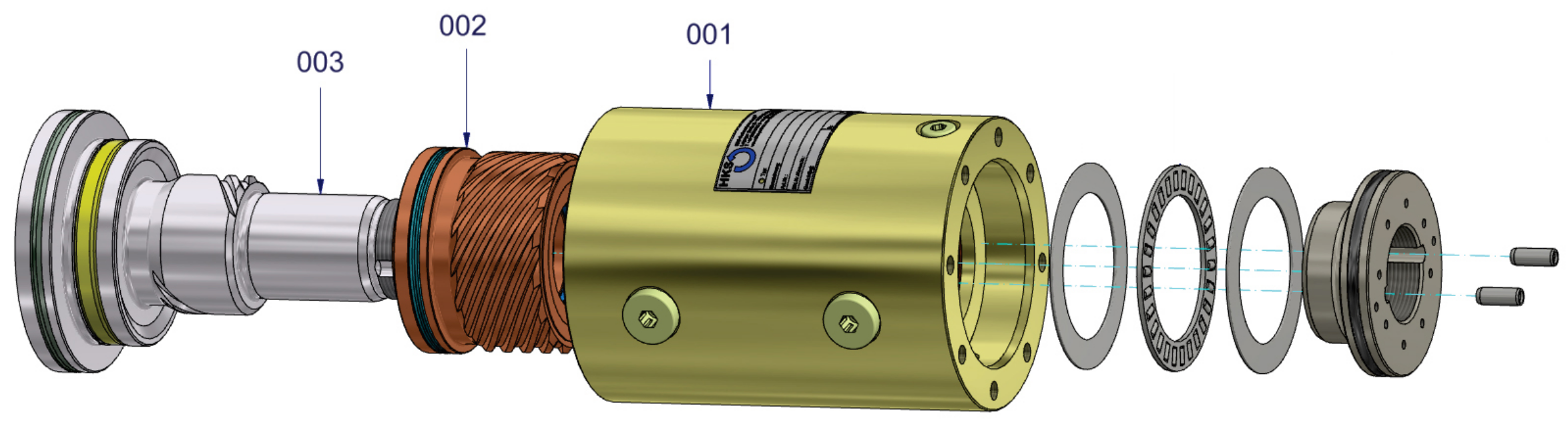
HHRA is referred to as a swing hydraulic cylinder. Figure 1 exhibits a diagram of the swing hydraulic cylinder mechanism of HKS Company [34], and its output angle has the range of [−90, 90] degrees. With HHRA, the rotary motion of the output shaft is achieved by the linear motion of the piston based on the double helical structure. Hence, the linear motion of the piston is converted into rotary motion by multiple counter-rotating high-helix threads on the housing (001), piston (002), and shaft (003).
Due to technical patent protection, detailed technical parameters are not available, so accurate mathematical models cannot be obtained. Based on this, the problem of how to develop a system model using the system identification method will be addressed.
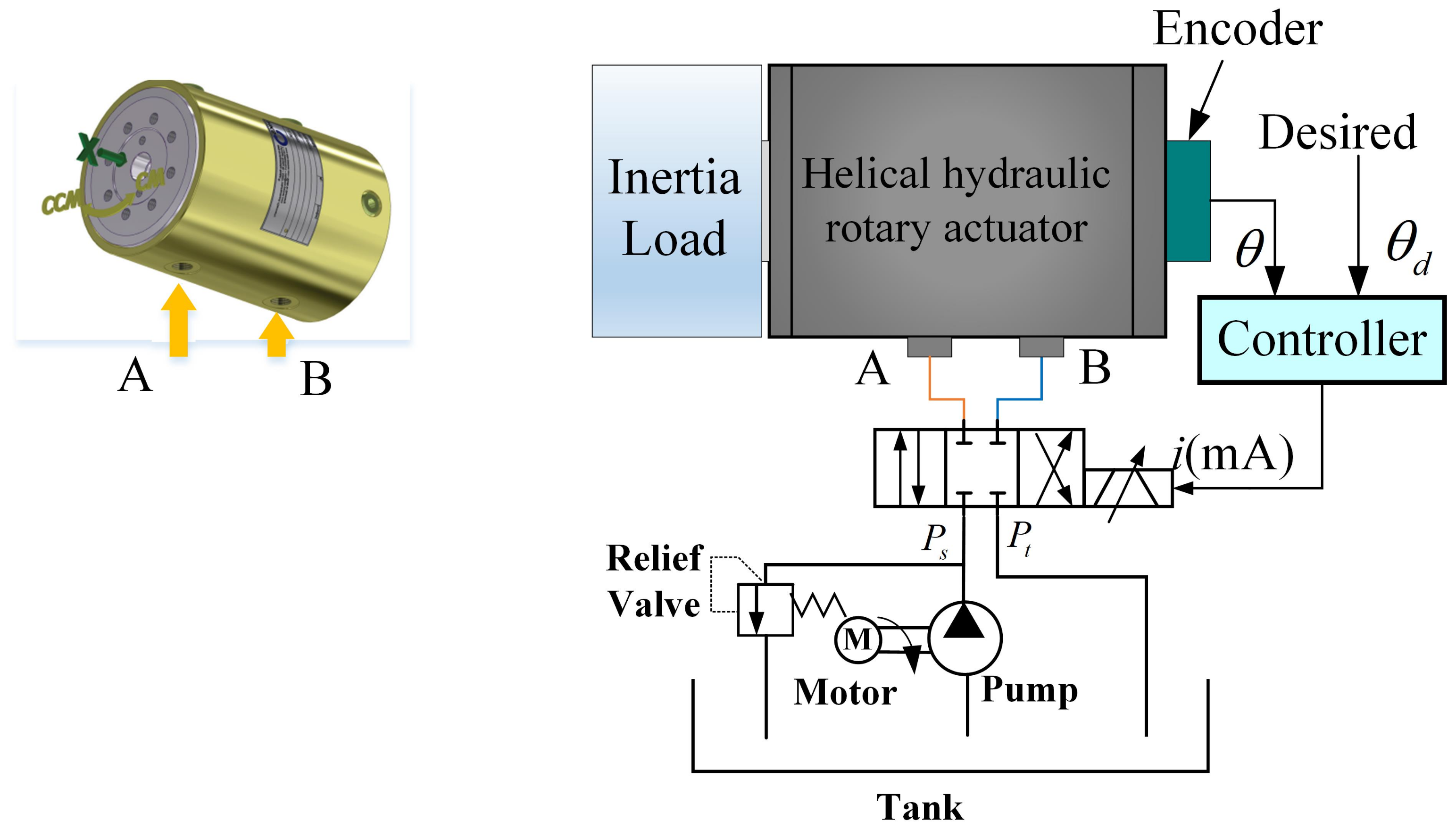
Figure 2 shows a schematic diagram of the valve-controlled HHRA, which mainly includes an encoder, a hydraulic actuator driven by a three-way four-port servo valve, and a controller. Labels A and B represent the inlet and outlet of the HHRA, respectively. The oil pressure is transmitted through the joint; otherwise, the actuator shaft would undergo rotational motion. Therefore, the linear motion of the piston is converted into rotational motion.
2.2. Model Design
To obtain a dynamic model of the valve controlled HHRAs, four fundamental formulas are required [35], namely flow continuity, load balance, output torque, and rotational balance formulas.
- (1)
- Flow continuity formula
Neglecting pressure loss and dynamics of the piping, the flow continuity formula for HHRA is given by [10]
where refers to the load flow; and are the supply flow rates; , is the piston displacement [2]; denotes the rotation angle; represents the leads of the two-stage helical pair; A denotes the effective area of the hydraulic cylinder piston; refers to the effective hydraulic fluid bulk modulus; is the coefficient of internal leakage; refers to the total control volume of the hydraulic actuator; and shows the load pressure difference, where and are forward chamber pressure and return chamber pressure, respectively.
- (2)
- Load balance formula
Dynamic characteristics of hydraulic power components are affected by load forces. The dynamics of the driving cylinder can be obtained as follows:
where m refers to the mass of the load; denotes the viscous friction coefficient; and F represents the axial force.
- (3)
- Rotational equilibrium formula
The load is assumed as a concentrated load, and then the torque balance equation can be expressed as follows:
where refers to the torque generated or developed by actuator, d denotes the reference diameter; and , where is the friction angle; and are the pitch angles of the helical pair. In addition, refers to the total viscous damping coefficient; J represents the total inertia of actuator and load; denotes the arbitrary load torque on shaft; and G refers to the torsional spring stiffness of the load, commonly assuming .
- (4)
- Flow equation of servo valve
In this study, it is assumed that the pump supply pressure is a constant and the return pressure is zero. The flow equation of servo valve can be expressed as follows [8]:
where denotes the linear relationship between the control signal and the position of the spool ; denotes the flow gain, therein represents the flow coefficient; refers to the valve area gradient; denotes the oil density; and refers to signum.
The flow equation for the servo valve in the forward/reverse direction is the same [36]. After full differential linearization is performed on the above equation and the incremental symbol is removed, the pressure-flow curve equation can be obtained as follows:
where and refer to the flow gain and flow pressure coefficient of the servo valve, respectively. Laplace transforms Equations (1)–(3) and (5) to get the fundamental equation of the HHRA, as follows:
- (5)
- Transfer function equation
According to Equations (6)–(9), the transfer function equation can be expressed as follows after the intermediate variables are eliminated:
where , , , .
Without consideration of the external interference, the transfer function between the rotation angle and the control input current can be expressed as follows (refer to the Appendix A for the detailed derivation process):
where .
2.3. Identification Model
Discretization of the transfer function is necessary for a system identification. A general system can be described by the follow differential equation:
where ; ; and refer to the input and output, respectively; denotes the delay time; and represents the disturbance. The discrete equation can be obtained based on Equation (11) using Tustin’s method:
According to the above equation, the differential equation of the system can be expressed as follows:
where and are parameters to be identified; denotes the observed value of the kth system output; refers to the actual value of the th system output; and represents the expected given value (i.e., system input) of the th system.
3. Methodology
3.1. Preliminary
Definition 1.
Let be a point in a dimensional space with , . The opposite point is defined as follows: .
Based on the above definitions, opposition scheme for learning can be formulated as follows.
Definition 2.
Opposition-based optimization (OBO) learning: is assumed as a fitness function to measure the candidate optimality. According to Definition 1, and can be obtained in every iteration; means point P can be replaced with .
3.2. GWO Algorithm
The GWO algorithm is inspired by the social leadership and hunting behavior of grey wolves in nature. The fittest solution is considered as alpha (). Consequently, the second and third best solutions are named as beta () and delta (), respectively. The rest of the candidate solutions are assumed to be omega (). The wolf hunting involves three main steps: hunting siege, hunting, and attacking prey.
- (1)
- Hunting siege
To simulate the hunting behavior of the grey wolves, the encircling operation can be represented as
where t indicates the current iteration; refers to the next location of the wolf; and denote the prey position and the position vector of a grey wolf at the current iteration t; D denotes the distance between the target prey and the grey wolves; and A and C represent the convergence coefficients, which can be calculated with the following equations:
where and represent two random vectors in [0, 1], components of the vectors decrease linearly from [2, 0], and denotes the maximum number of iterations.
- (2)
- Hunting
To mathematically model the hunting behavior of grey wolves, the other wolves are obliged to follow the position of the three best solutions , , and . The hunting behavior can be expressed as follows:
Positions of the individual grey wolf are updated using following equation:
- (3)
- Attacking
In this step, exploration and exploitation are guaranteed by the adaptive values of a and A; a is a distance control parameter, which decides the distance approaching the prey; A balances the exploration and exploitation capabilities of the GWO algorithm. Exploration is promoted when , whereas there is emphasis on exploitation when . When , a repeated attack will be carried out, and a return attack will be stopped.
3.3. Modified Differential Evolution
The classical DE algorithm consists of three basic steps: mutation, crossover, and selection.
- (1)
- Mutation
In this study, based on a mutation operator DE/best/1 [37] of classical DE, the improved mutant individual will be updated as follows:
where refers to the scaling factor, which is a fixed constant that is used to add diversity to the search; denotes the differential weight or scaling factor, larger values for F result in higher diversity in generation population and lower values result in faster convergence, and represents the global best wolf with a minimum during the iteration. In addition, and are two randomly chosen indices () in the range , and denotes the population size.
- (2)
- Crossover
A modified crossover operation is introduced after the mutation to enhance the potential diversity of the population. The binomial crossover is represented as follows:
where denotes the crossover rate in the range [0, 1], and [0, 1] refers to a uniformly distributed random number; denotes a randomly chosen index. The following equation can be selected to check and process the boundary condition.
where a and b are the pre-specified lower and upper limit, respectively; and denotes a uniform random number in the range [0, 1].
- (3)
- Selection
A one-to-one greedy selection between a parent and its corresponding offspring can judge whether the target or the trial vector survives to the next generation. The minimization can be stated as follows:
where denotes the fitness function; and denote the trial vector and the current target vector, respectively.
3.4. GWO with DE Hybrid Algorithm
The GWO algorithm has been verified to show high superiority in many fields, but it inevitably faces some deficiency such as local optimum, slow calculation speed, and low accuracy. Herein, based on the previous sections about GWO and DE, a novel hybrid approach, H-GWO, is proposed to enhance the search performance.
- (1)
- Initialization scheme
Initial value of the population can govern the quality of the final solution and the convergence speed of the SI algorithm [38]. In this direction, a hybrid population initialization scheme is designed by combining OBO and chaotic maps.
A randomly distributed population (n refers to the population size) is obtained based on the tent chaotic maps. Then, chaotic sequences in (0, 1) will be generated in the following form:
where ; represents the value of the kth mapping function. A randomly distributed population can be obtain by
where and denote the maximum and minimum limits, respectively. Opposite population is calculated by the following equation:
Here, the final initial population is determined by selecting the best n individual solutions evaluated from the combined population set of
where ⊗ represents the optimal selection operation, and the detailed steps are described as follows: First, the parent population is sorted after duplicate data are removed in a non-descending order. Then, based on the fitness function, the parental population of grey wolves is sorted from smallest to largest, and the first n individual positions in the grey wolf parent population are found and determined as the initial population position.
- (2)
- Population diversification strategy
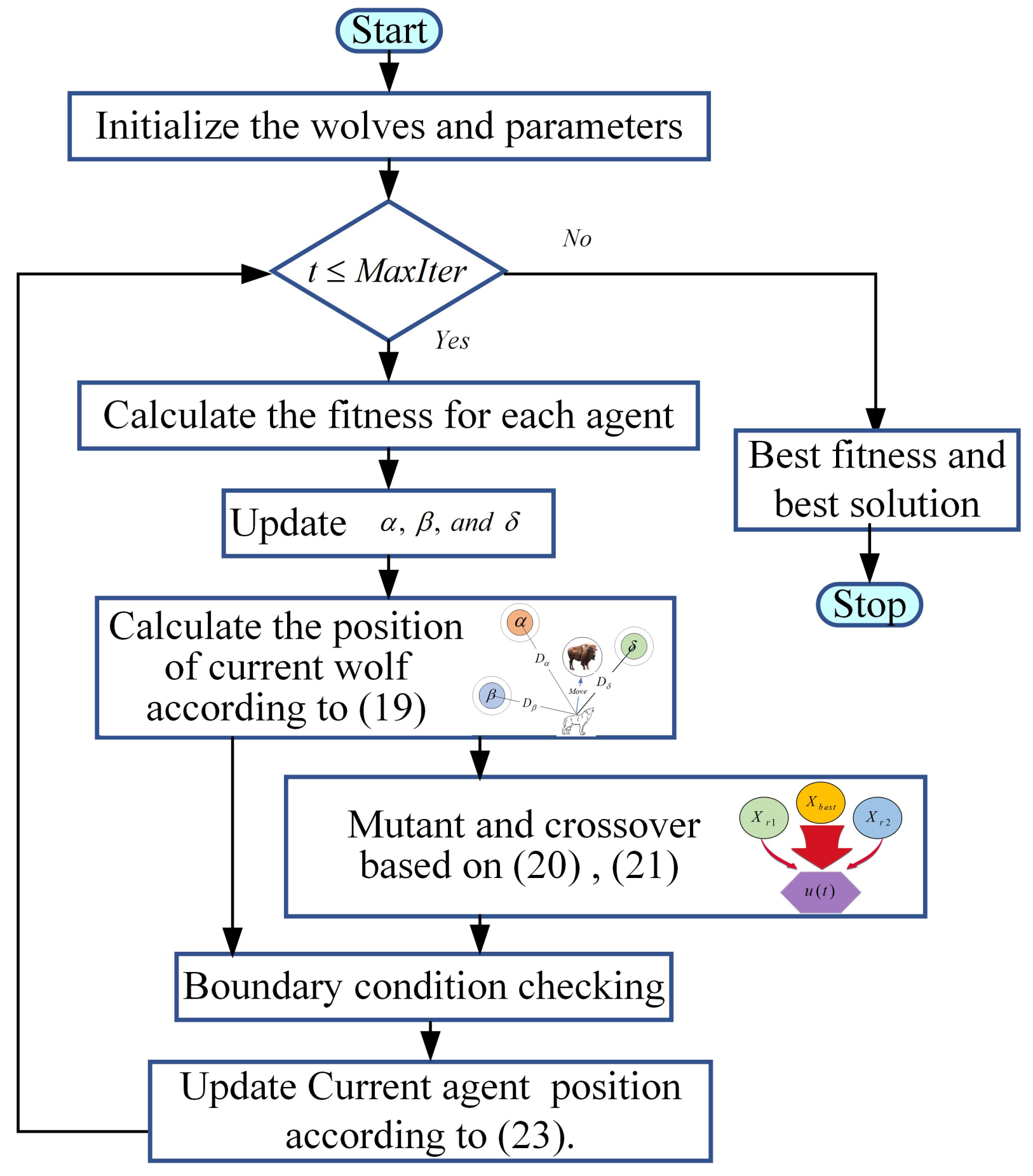
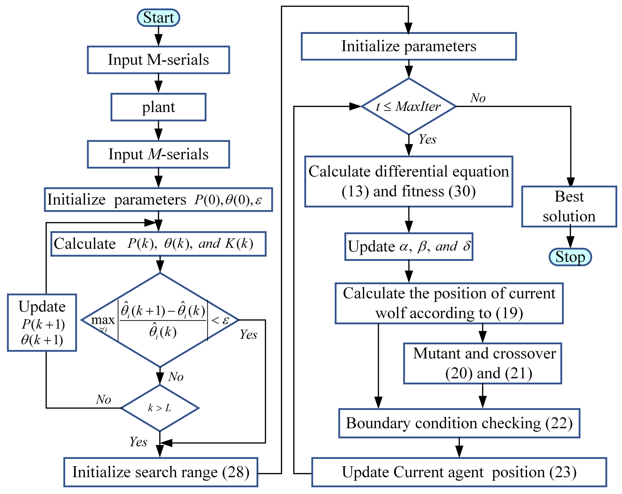
The opposition-based differential evolution (ODE) is introduced to enhance the potential diversity of the population. The mutation, crossover, and selection under the DE algorithm involve the update of the new wolf position. The H-GWO algorithm can be described by the following steps, and its flowchart is presented in Figure 3.
- Step 1.
- Initializing parameters and values of a, A, and C as well as the crossover rate , scaling factor F, and maximum number of iterations ;
- Step 2.
- Initializing a population of n agents position randomly according to Equation (27);
- Step 3.
- Calculating the fitness f for all individuals;
- Step 4.
- Updating , , and ;
- Step 5.
- Step 6.
- Calculating the position of the current wolf according to Equation (19);
- Step 7.
- Step 8.
- Checking and processing the boundary condition according to Equation (22);
- Step 9.
- Updating position of the current agent according to Equation (23);
- Step 10.
- Returning the Step 3 at stopping criteria , or otherwise going to next step;
- Step 11.
- Returning the best fitness and the best solution .
3.5. Verification and Discussion of H-GWO Algorithm
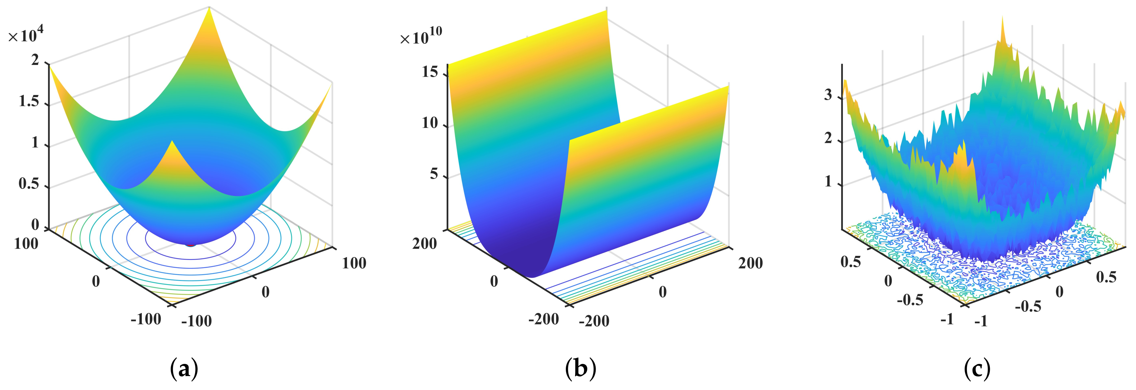
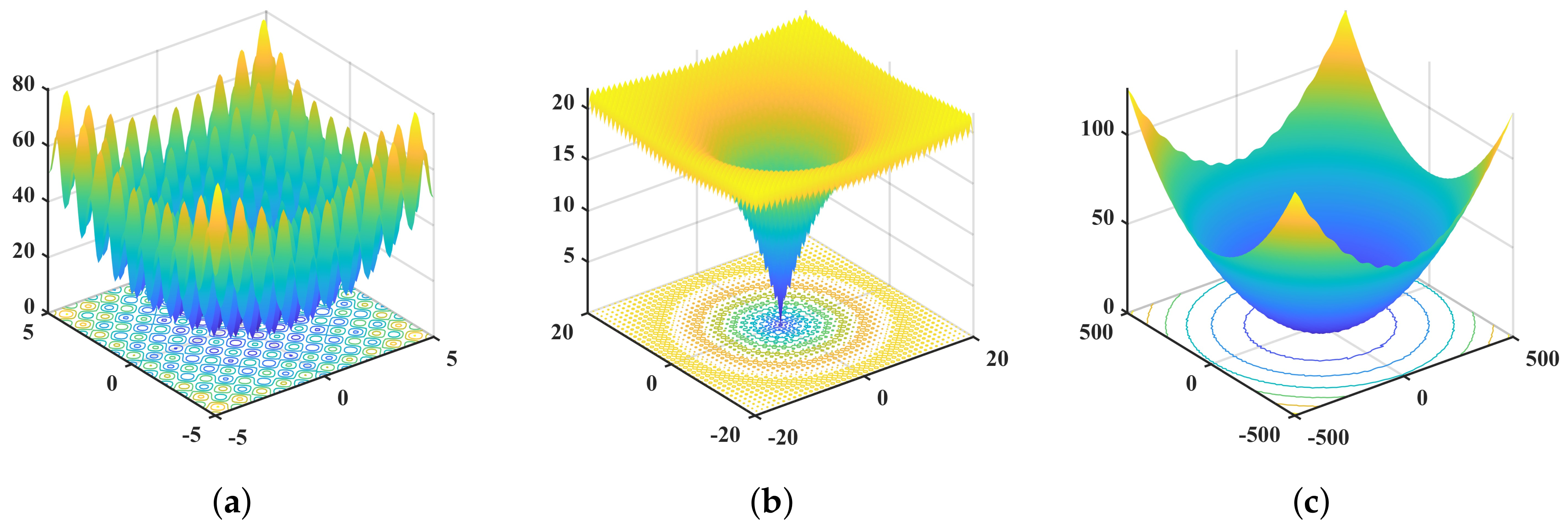
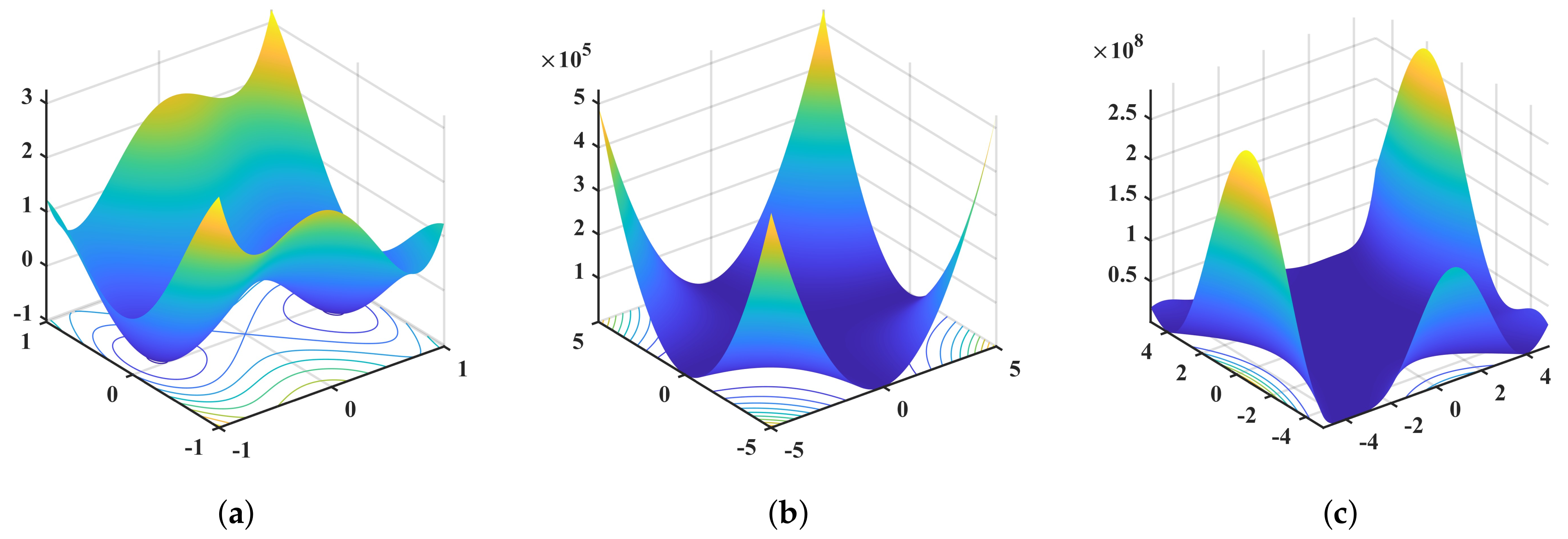
In this section, nine classic and popular benchmark functions are employed to test its performance [24]. They can be divided into three groups: unimodal benchmark functions (Figure 4), multimodal benchmark functions (Figure 5), and fixed-dimensional multimodal benchmark functions (Figure 6), as listed in Table 1. In the Table 2, Dim indicates dimension of the function, Range is the boundary of the function’s search space, and represents the optimal value.
The H-GWO algorithm is compared with PSO, GWO, and DE algorithms to illustrate its better performance. For ease of understanding, the parameter configurations of the above four methods are described as follows. Additionally, the same population size and the same maximum number of iterations are set for all algorithms.
- (1)
- PSO:
Maximum speed , inertia weight , and acceleration coefficient .
- (2)
- GWO:
Parameters , .
- (3)
- DE:
Scaling factor crossover probability .
- (4)
- H-GWO:
Scaling factor , crossover probability , and .
The all algorithm is run 30 times on each benchmark function. Experimental results consist of statistical parameters such as mean and standard deviation (St.dev), as listed in Table 2.
- (1)
- Discussion on exploitation and exploration
Table 2 shows the Average and St.dev results for the benchmark functions. According to the results of in Table 2, the H-GWO algorithm can provide very competitive results. The unimodal benchmark function is very suitable for testing the utilization of the algorithm. These results confirm the superior performance of the H-GWO algorithm in exploiting the optimality. Compared with the unimodal benchmark function, the multimodal benchmark function is subjected to many local optima, so it is suitable for testing the benchmark exploration performance. In addition, Table 2 reveals that the H-GWO algorithm can achieve competitive results on multimodal benchmark functions. Therefore, the proposed H-GWO algorithm outperforms the GWO, PSO, and DE algorithms on most of the multimodal benchmark functions, demonstrating its advantages in terms of exploration.
- (2)
- Local minima avoidance
The multimodal benchmark function shows multiple local minima, so it can be used to test the local minima avoidance. Again, Table 2 suggests that the proposed algorithm exhibits superior convergence performance on the multi-modal benchmark function, reflecting its good performance on local minimum avoidance simultaneously.
In summary, the experimental results validate the performance of the proposed algorithm in computing various benchmark functions compared to other meta-heuristic algorithms. Next, the proposed algorithm is further adopted for parameter identification in engineering applications.
4. Application of H-GWO Algorithm for Parameter Identification
In this section, the H-GWO algorithm proposed in this study is for parameter identification of the HHRA, that is, to identify unknown parameters from known system inputs and outputs. For this purpose, a hybrid identification algorithm combining FFRLS and H-GWO algorithms is proposed.
4.1. Parameter Identification Strategy
In this section, the estimated expansion function is designed based on the FFRLS as the initial search range. The algorithmic strategy of forgetting factor recursive least squares (FFRLS) is to revise the parameter estimates based on new data while gradually forgetting or attenuating the influence of older data. The iterative update equation of the FFRLS algorithm can be expressed as follows:
where and are initial values, represents a real positive constant, and refers to a sufficiently small positive real vector; denotes a forgetting factor, and the time-varying forgetting factor is , , . With the above FFRLS estimation, the identification result shows a low accuracy. Here, the initial search range expansion function is introduced as follows by referring to the above parameter results as interim parameter estimation:
In the above equation, refers to the expansion space gain coefficient. As for the H-GWO algorithm, the estimated expansion function is undertaken as the initial search space.
In short, Figure 7 illustrates the improved identification algorithm that combines the FFRLS and H-GWO algorithms.
4.2. Accuracy Index
There are three commonly used criteria with definitions as follows:
Definition 3.
Integral of the time weighted absolute error (ITAE) integrates the absolute error multiplied by the time over time, which is defined as follows:
Herein, the ITAE index is chosen as the fitness function.
Definition 4.
Mean squared error (MSE) represents the mean of the squared measurement errors of an estimator, which is expressed as follows. The smaller the value, the higher the degree of approximation.
where and represent the actual and predicted value, respectively; and n is the total length of the data.
Definition 5.
The variance accounted for (VAF) refers to the percentage of a variance ratio, which is often adopted to verify the model correctness. VAF between and for the ith component is defined as follows:
where is the variance.
4.3. Results and Analysis
In this section, the parameter identification and experimental results will be presented for a hydraulic system.
- Experiment setup
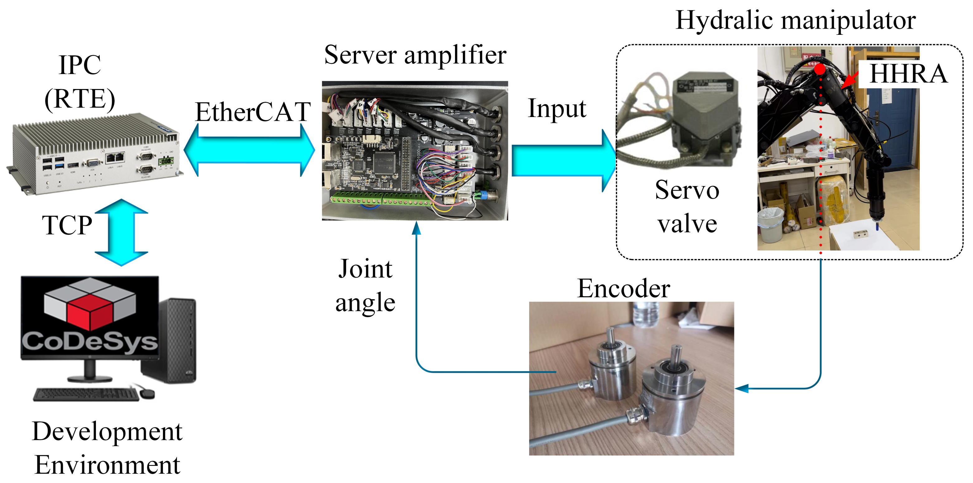
The platform consists of a HHRA (HKS), a servo valve (HY110), a rotary encoder (SSI), servo amplifier, and industrial personal computer (IPC). The sampling time is 250 Hz (4 ms), and the duration is taken as 20 s. The experimental platform is shown in Figure 8. CodeSys software is adopted in the development environment.
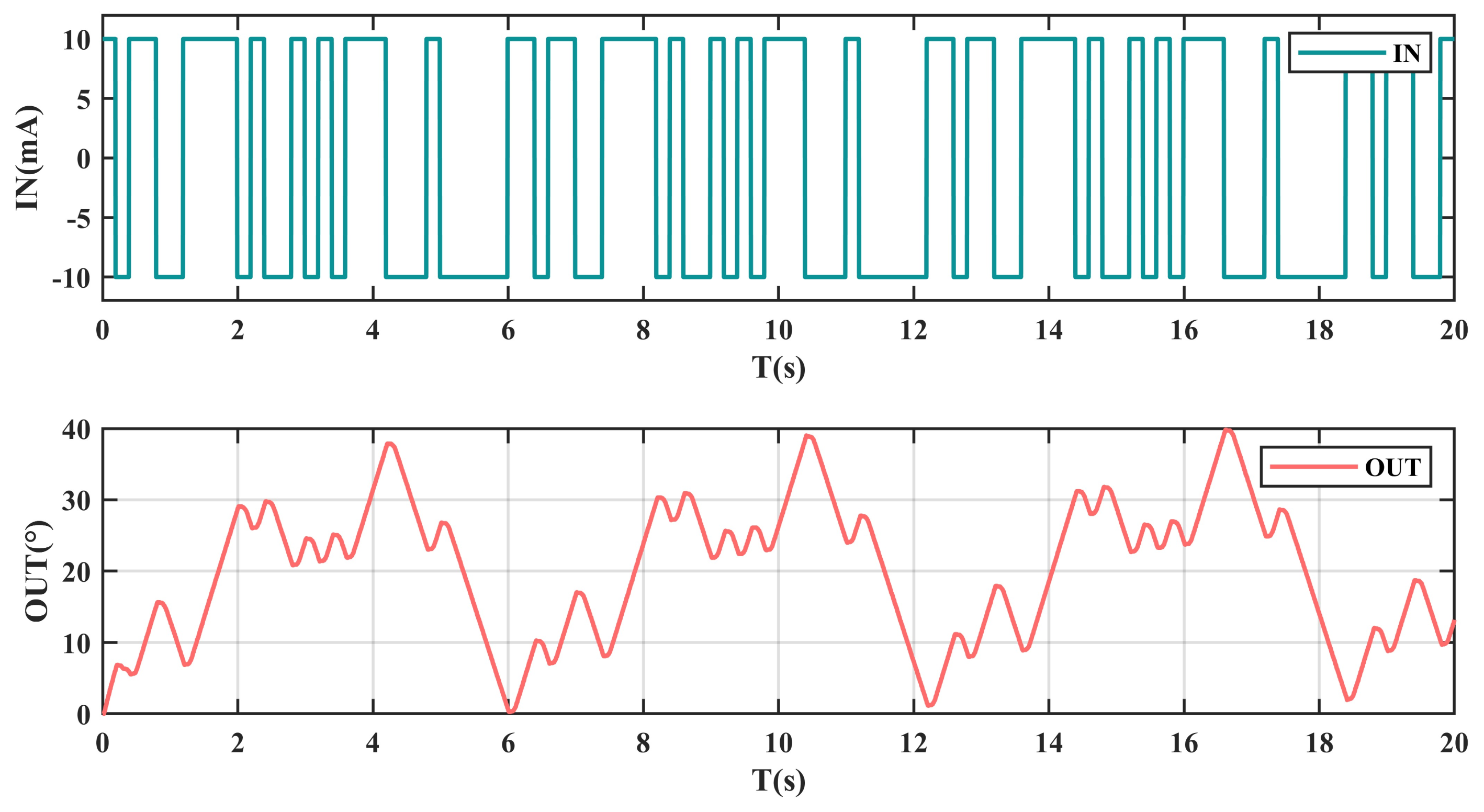
The experimental process is as follows: First, an irregular continuous step control signal (current value) is sent as the input to the servo system through an IPC. Then, the feedback value of the HHRA is collected as the output signal through an encoder. Therein, the 4th-order inverse M sequence is selected as the excitation signal in this study,
The input and output collected in the experiment are displayed in Figure 9. Thereof, the top sub-picture is the input signal, and the bottom sub-picture is the corresponding system output.
- B.
- Experimental Results
Herein, the proposed method is compared with LS, RLS, FFRLS, PSO, and GWO. To facilitate understanding, the expressions of the above methods are presented as follows.
- (1)
- LS method:
- (2)
- RLS method
- (3)
- FFRLS method
- (4)
- PSO method
- (5)
- GWO method
The GWO method is presented in Equations (14)–(19), where ; ; Initial search range [−5, 5]; and , .
- (6)
- FFRLS and H-GWO hybrid method
The method described in Section 4 is applied here, where population size ; and maximum iterations . Scaling factor ; crossover probability ; and . Other parameters are the same as in (3).
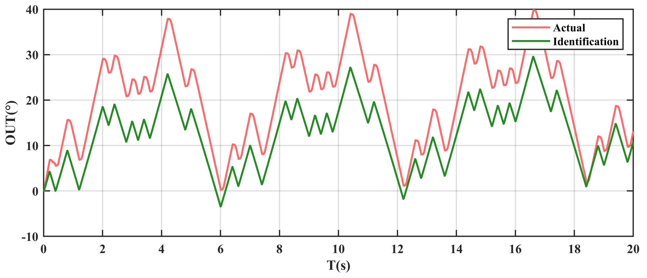
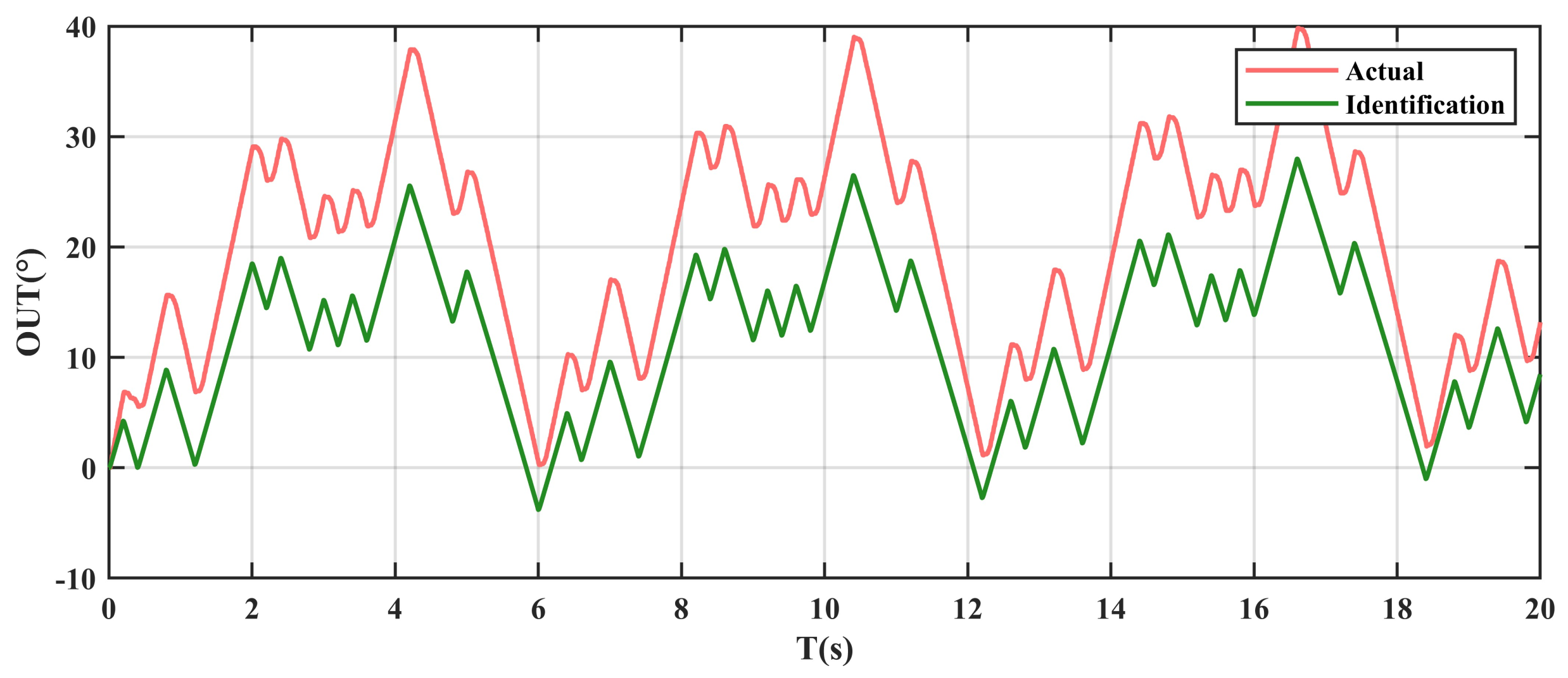
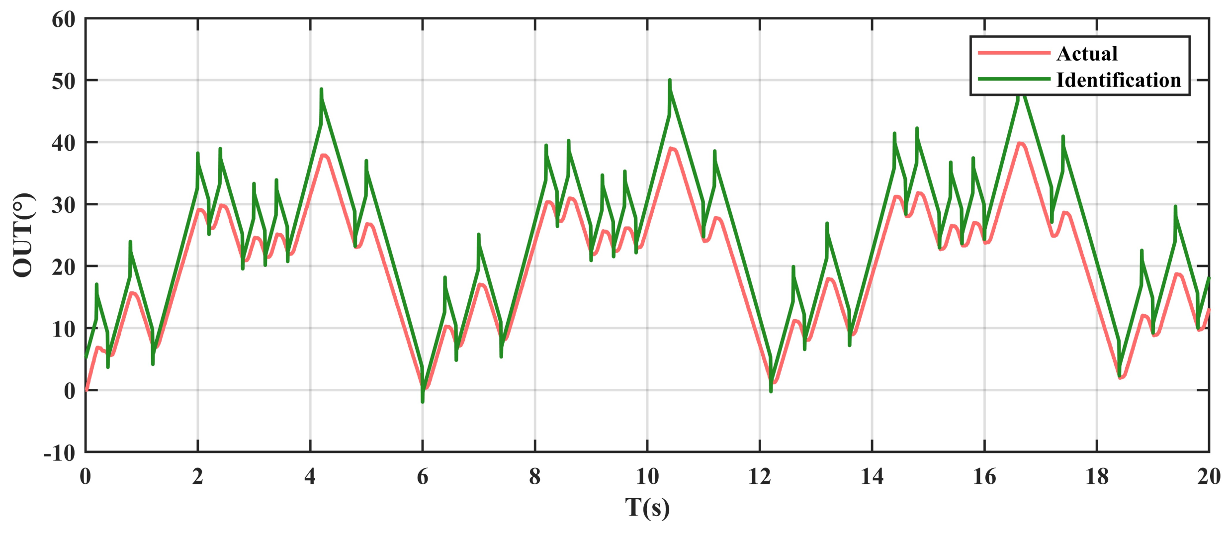
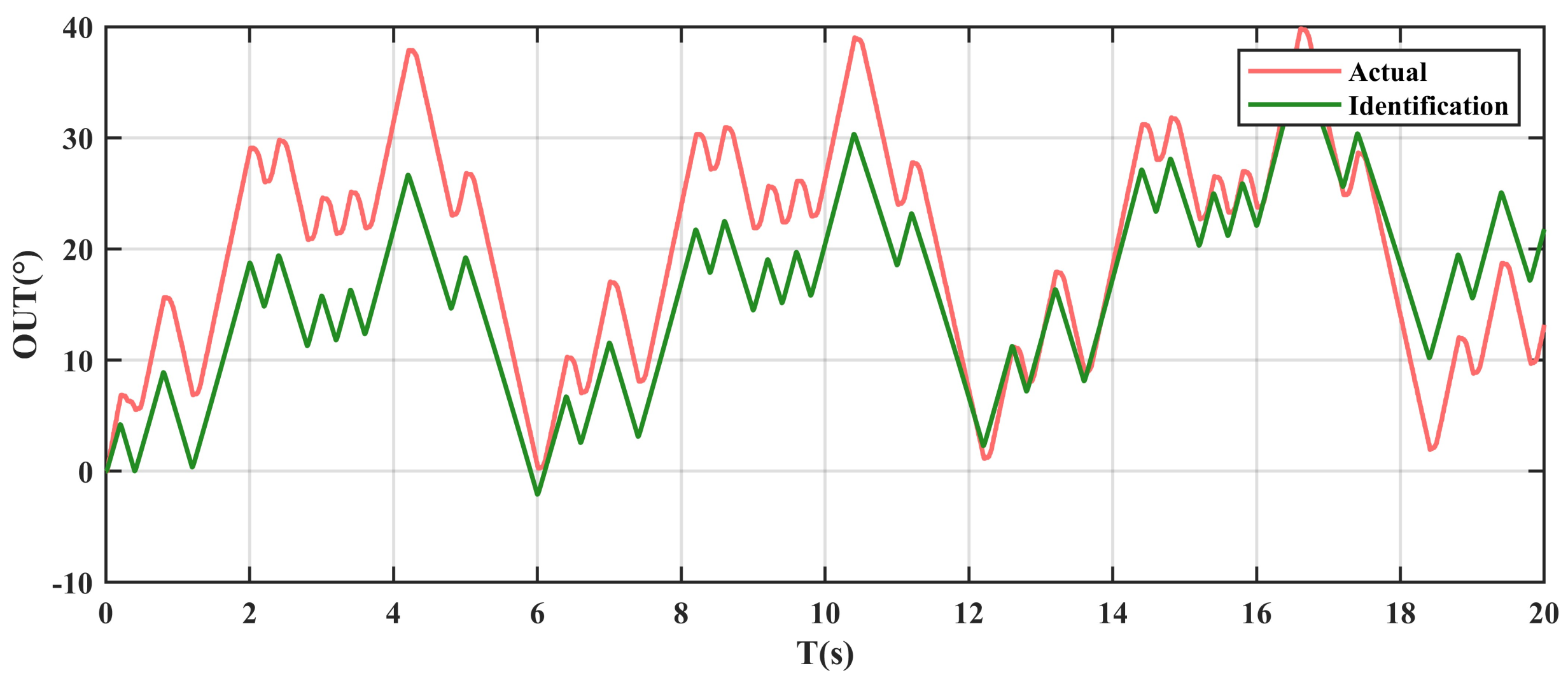
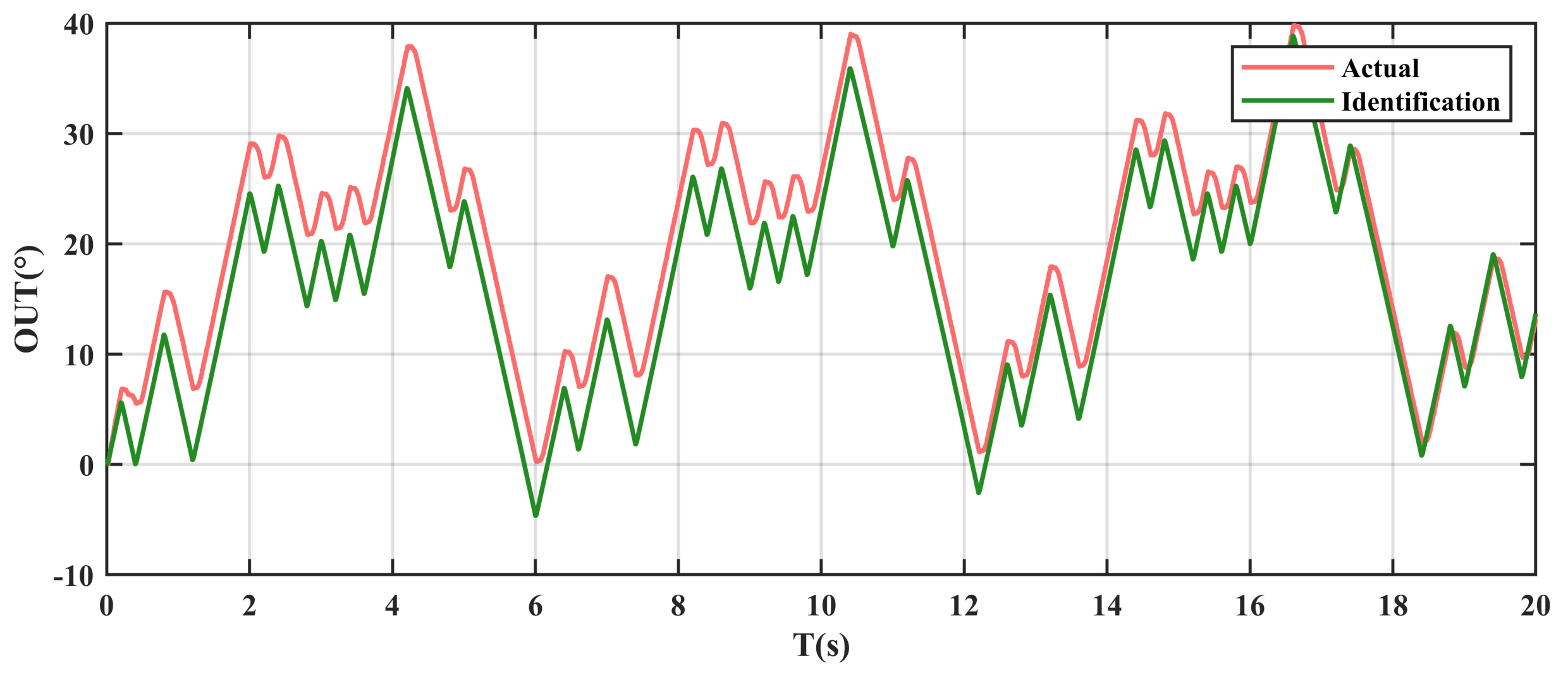
The parameters MSE, VAF, and number of iterations (NOI) are employed to better present the superior performance of the proposed method. Figure 10, Figure 11, Figure 12, Figure 13, Figure 14 and Figure 15 represent the identification result of LS, RLS, FFRLS, PSO, GWO, and the proposed algorithm, respectively. The figures suggest that identification accuracy of the proposed algorithm is significantly higher than that of other algorithms.
From Figure 10, Figure 11 and Figure 12, it can be seen that the identification results based on least squares has very similar results. However, from the VAF results in Table 3, it can be seen that FFRLS has improved accuracy relative to RLS, but the overall accuracy is still not good enough, especially with the MSE results having larger values. The reason for this may be due to the insufficient amount of data in the experiment, but increasing the amount of data will undoubtedly increase the computational time.
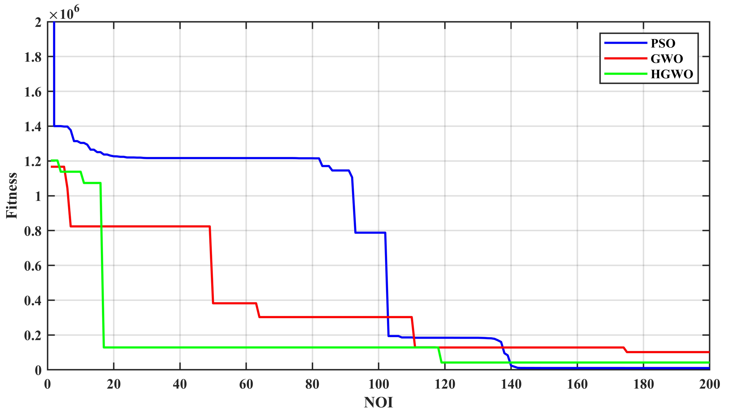
Table 3 shows the MSE, VAF, and NOI indexes of the three identification methods for comparison. The proposed algorithm exhibits a higher identification accuracy according to the data listed in Table 3 and Definitions 3 and 4. In addition, the proposed algorithm shows fewer NOI. In Figure 16, the convergence of the fitness function is presented, demonstrating that the proposed method achieves faster convergence without premature convergence.
Remark 1.
From the results in Figure 13 and Table 3, it can be seen that the PSO algorithm also has a high identification accuracy, but the identification result has an impact at the peak, which is inconsistent with the actual system. The algorithm proposed in this paper combines the advantages of FFRLS and H-GWO to achieve higher accuracy. In particular, as the amount of data increases, the accuracy is further improved, as shown in Figure 15.
5. Conclusions
The H-GWO algorithm combining GWO and DE is presented in this study. In addition, the OBO learning technology is fused to update the GWO population, increasing the diversity of the population, avoiding the local optimum, and making an appropriate compromise between exploration and exploitation. A parameter identification algorithm combining FFRLS and the proposed H-GWO algorithm is designed for parameter identification of HHRA. In addition, its validity and accuracy are proved by simulation and experimental results. System identification is of great significance in control engineering and system analysis. It provides a theoretical basis for system understanding, system analysis, controller design, system optimization, etc. Through system identification, the behavior characteristics of the system can be deeply understood, and then the system can be better analyzed, controlled, and optimized. Practical control problems for which the identification model is used will be considered in the future.
Author Contributions
Conceptualization, Y.Z., Y.L. (Yixiang Liu) and R.S. (Ruyue Sun); methodology, Y.Z. and R.S. (Ruyue Sun); software, Y.Z.; validation, Y.Z., R.S. (Ruyue Sun) and Y.L. (Yixiang Liu); investigation, Y.W. and Y.L. (Yixiang Liu); resources, Y.Z. and Y.L. (Yixiang Liu); data curation, Y.Z. and R.S. (Ruyue Sun); writing—original draft preparation, Y.Z. and R.S. (Ruyue Sun); writing—review and editing, Y.Z. and R.S. (Ruyue Sun); visualization, Y.W. and Y.L. (Yixiang Liu); supervision, Y.L. (Yibin Li) and R.S. (Rui Song); project administration, R.S. (Rui Song); funding acquisition, R.S. (Rui Song). All authors have read and agreed to the published version of the manuscript.
Funding
This research was funded by the National Key Research and Development Program of China (2022YFC2604004), the Key Research and Development Program of Hebei Province under Grant 20311803D, and the Natural Science Foundation of China under Grant U20A20201.
Data Availability Statement
The datasets of the current study are available from the corresponding author upon reasonable request.
Conflicts of Interest
The authors declare no conflict of interest.
Appendix A
According to Equations (6) and (9), we can obtain
The load pressure difference can be obtained:
According to Equation (3), we can obtain
Substitute Equation (8) into Equation (A3):
Substitute Equation (A2) into Equation (A4):
By further rearranging the above expression, we can get
Finally, we can obtain
References
- Jelali, M.; Kroll, A. Hydraulic Servo-Systems: Modelling, Identification, and Control; Springer Science & Business Media: Berlin/Heidelberg, Germany, 2002. [Google Scholar]
- Zhang, K.; Zhang, J.; Gan, M.; Zong, H.; Wang, X.; Huang, H.; Xu, B. Modeling and Parameter Sensitivity Analysis of Valve-Controlled Helical Hydraulic Rotary Actuator System. Chin. J. Mech. Eng. 2022, 35, 66. [Google Scholar] [CrossRef]
- Zhu, T.; Xie, H.; Yang, H. Design and tracking control of an electro-hydrostatic actuator for a disc cutter replacement manipulator. Autom. Constr. 2022, 142, 104480. [Google Scholar] [CrossRef]
- Heng, L. Mobile Machinery Cylinders-Aerial Work Platform Cylinder. Available online: https://www.henglihydraulics.com/en/application/ApplicationCenter (accessed on 29 November 2021).
- Parker. Helac Products|Parker Cylinder Division. Available online: https://promo.parker.com/promotionsite/helac/us/en/products (accessed on 29 November 2021).
- Schwenzer, M.; Ay, M.; Bergs, T.; Abel, D. Review on model predictive control: An engineering perspective. Int. J. Adv. Manuf. Technol. 2021, 117, 1327–1349. [Google Scholar] [CrossRef]
- Tran, D.T.; Do, T.C.; Ahn, K.K. Extended high gain observer-based sliding mode control for an electro-hydraulic system with a variant payload. Int. J. Precis. Eng. Manuf. 2019, 20, 2089–2100. [Google Scholar] [CrossRef]
- Yao, J.; Jiao, Z.; Ma, D. Extended-state-observer-based output feedback nonlinear robust control of hydraulic systems with backstepping. IEEE Trans. Ind. Electron. 2014, 61, 6285–6293. [Google Scholar] [CrossRef]
- Yao, J.; Jiao, Z.; Ma, D.; Yan, L. High-accuracy tracking control of hydraulic rotary actuators with modeling uncertainties. IEEE/ASME Trans. Mechatron. 2013, 19, 633–641. [Google Scholar] [CrossRef]
- Sadeghieh, A.; Sazgar, H.; Goodarzi, K.; Lucas, C. Identification and realtime position control of a servo-hydraulic rotary actuator by means of a neurobi-ologically motivated algorithm. ISA Trans. 2012, 51, 208–219. [Google Scholar] [CrossRef]
- Katoch, S.; Chauhan, S.S.; Kumar, V. A review on genetic algorithm: Past, present, and future. Multi-Media Tools Appl. 2021, 80, 8091–8126. [Google Scholar] [CrossRef]
- Marini, F.; Walczak, B. Particle swarm optimization (PSO): A tutorial. Chemom. Intell. Lab. Syst. 2015, 149, 153–165. [Google Scholar] [CrossRef]
- Das, S.; Suganthan, P.N. Differential evolution: A survey of the state-of-the-art. IEEE Trans. Evol. Comput. 2010, 15, 4–31. [Google Scholar] [CrossRef]
- Kim, J.H.; Myung, H. Evolutionary programming techniques for constrained optimization problems. IEEE Trans. Evol. Comput. 1997, 1, 129–140. [Google Scholar]
- Lin, Q.; Ma, Y.; Chen, J.; Zhu, Q.; Coello, C.A.C.; Wong, K.C.; Chen, F. An adaptive immune-inspired multi-objective algorithm with multiple differential evolution strategies. Inf. Sci. 2018, 430, 46–64. [Google Scholar] [CrossRef]
- Storn, R.; Price, K. Differential evolution-a simple and efficient heuristic for global optimization over continuous spaces. J. Glob. Optim. 1997, 11, 341. [Google Scholar] [CrossRef]
- Ozer, A.B. CIDE: Chaotically initialized differential evolution. Expert Syst. Appl. 2010, 37, 4632–4641. [Google Scholar] [CrossRef]
- Ahmad, M.F.; Isa, N.A.M.; Lim, W.H.; Ang, K.M. Differential evolution: A recent review based on state-of-the-art works. Alex. Eng. J. 2022, 61, 3831–3872. [Google Scholar] [CrossRef]
- Gong, W.; Cai, Z. Differential evolution with ranking-based mutation operators. IEEE Trans. Cybern. 2013, 43, 2066–2081. [Google Scholar] [CrossRef]
- Wolpert, D.H.; Macready, W.G. No free lunch theorems for optimization. IEEE Trans. Evol. Comput. 1997, 1, 67–82. [Google Scholar] [CrossRef]
- Dorigo, M.; Stützle, T. Ant Colony Optimization: Overview and Recent Advances; Springer International Publishing: Berlin/Heidelberg, Germany, 2019. [Google Scholar]
- Abedinia, O.; Amjady, N.; Ghasemi, A. A new metaheuristic algorithm based on shark smell optimization. Complexity 2016, 21, 97–116. [Google Scholar] [CrossRef]
- Karaboga, D.; Gorkemli, B.; Ozturk, C.; Karaboga, N. A comprehensive survey: Artificial bee colony (ABC) algorithm and applications. Artif. Intell. Rev. 2014, 42, 21–57. [Google Scholar] [CrossRef]
- Mirjalili, S.; Mirjalili, S.M.; Lewis, A. Grey Wolf Optimizer. Adv. Eng. Softw. 2014, 69, 46–61. [Google Scholar] [CrossRef]
- Saremi, S.; Mirjalili, S.Z.; Mirjalili, S.M. Evolutionary population dynamics and grey wolf optimizer. Neural Comput. Appl. 2015, 26, 1257–1263. [Google Scholar] [CrossRef]
- Mirjalili, S.; Saremi, S.; Mirjalili, S.M.; Coelho, L.D.S. Multi-objective grey wolf optimizer: A novel algorithm for multicriterion optimization. Expert Syst. Appl. 2016, 47, 106–119. [Google Scholar] [CrossRef]
- Faris, H.; Aljarah, I.; AlBetar, M.A.; Mirjalili, S. Grey wolf optimizer: A review of recent variants and applications. Neural Comput. Appl. 2018, 30, 413–435. [Google Scholar] [CrossRef]
- Wang, J.; Xu, Y.P.; She, C.; Bagal, H.A. Optimal parameter identification of SOFC model using modified gray wolf optimization algorithm. Energy 2022, 240, 122800. [Google Scholar] [CrossRef] [Green Version]
- Yang, Y.; Li, C.; Ding, H.F. Modeling and Parameter Identification of High Voltage Pulse Rock-breaking Discharge Circuit. J. Mech. Eng. 2022, 58, 243–251. [Google Scholar]
- Ladi, S.K.; Panda, G.K.; Dash, R.; Ladi, P.K.; Dhupar, R. A novel grey wolf optimisation based CNN classifier for hyper-spectral image classification. Multimed. Tools Appl. 2022, 81, 28207–28230. [Google Scholar] [CrossRef]
- Li, S.X.; Wang, J.S. Dynamic modeling of steam condenser and design of PI controller based on grey wolf optimizer. Math. Probl. Eng. 2015, 2015, 120975. [Google Scholar] [CrossRef]
- Achom, A.; Das, R.; Pakray, P. An improved Fuzzy based GWO algorithm for predicting the potential host receptor of COVID-19 infection. Comput. Biol. Med. 2022, 151, 106050. [Google Scholar] [CrossRef]
- Mohammed, H.; Rashid, T. A novel hybrid GWO with WOA for global numerical optimization and solving pressure vessel design. Neural Comput. Appl. 2020, 32, 14701–14718. [Google Scholar] [CrossRef]
- HKS. HKS—Products. Available online: https://www.hks-partner.com/en/products (accessed on 29 November 2021).[Green Version]
- Song, B.L. Dynamic Characteristics Study of Screw Oscillating Hydraulic Cylinder; Central South University: Changsha, China, 2011. [Google Scholar]
- Ye, X.H. Research on Modeling and Control Method of Valve-Controlled Asymmetrical Cylinder System; Hefei University of Technology: Hefei, China, 2014. [Google Scholar] [Green Version]
- Gupta, S.; Deep, K.; Moayedi, H.; Foong, L.K.; Assad, A.L. Sine cosine grey wolf optimizer to solve engineering design problems. Eng. Comput. 2021, 37, 3123–3149. [Google Scholar] [CrossRef] [Green Version]
- Ahmad, M.F.; Isa, N.A.M.; Lim, W.H.; Ang, K.M. Differential evolution with modified initialization scheme using chaotic oppositional based learning strategy. Alex. Eng. J. 2022, 61, 11835–11858. [Google Scholar] [CrossRef]
Figure 1.
Structural diagram of HHRA [34].
Figure 1.
Structural diagram of HHRA [34].

Figure 2.
Architecture of the valve-controlled HHRA.

Figure 3.
Flowchart of H-GWO.

Figure 4.
Two—dimensional versions of unimodal benchmark functions: (a) ; (b) ; (c) .

Figure 5.
Two—dimensional versions of multimodal benchmark functions: (a) ; (b) ; (c) .

Figure 6.
Two−dimensional version of fixed-dimension multimodal benchmark functions: (a) ; (b) ; (c) .
Figure 6.
Two−dimensional version of fixed-dimension multimodal benchmark functions: (a) ; (b) ; (c) .

Figure 7.
Flowchart of parameter identification using H-GWO.

Figure 8.
Physical prototype workbench.

Figure 9.
Input and output.

Figure 10.
Comparison of identification results using LS.

Figure 11.
Comparison of identification results using RLS.

Figure 12.
Comparison of identification results using FFRLS.

Figure 13.
Comparison of identification results using PSO.

Figure 14.
Comparison of identification results using GWO.

Figure 15.
Comparison of identification results using the proposed method.

Figure 16.
Comparison of convergence.


Table 1.
Nine benchmark test functions [24].
Table 1.
Nine benchmark test functions [24].
| Function | Dim | Range | |
|---|---|---|---|
| Unimodal benchmark functions | |||
| 30 | [−100, 100] | 0 | |
| 30 | [−30, 30] | 0 | |
| 30 | [−1.28, 1.28] | 0 | |
| Multimodal benchmark functions | |||
| 30 | [−5.12, 5.12] | 0 | |
| 30 | [−30, 30] | 0 | |
| 30 | [−600, 600] | 0 | |
| Fixed-dimension Multimodal benchmark functions | |||
| 2 | [−5, 5] | −1.0316 | |
| 4 | [−5, 5] | 0.0003 | |
| 2 | [−2, 2] | 3 |
Table 2.
Experimental results (average, standard) of benchmark functions.
| Function | PSO | GWO | DE | H-GWO | ||||
|---|---|---|---|---|---|---|---|---|
| Average | St. dev | Average | St. dev | Average | St. dev | Average | St. dev | |
| 5.107963 | 2.045059 | 0.002765 | 1.3874 | 4.0215 | ||||
| 68.341611 | 39.848151 | 27.960574 | 0.00391 | 28.940232 | 0.02895 | 25.901103 | 0.671705 | |
| 8.714045 | 6.275347 | 0.003067 | 0.003762 | 0.030475 | 0.039981 | 0.001465 | ||
| 38.039407 | 31.421778 | 1.544107 | 35.973785 | 81.892454 | 17.961906 | 0.513119 | ||
| 3.080351 | 0.351753 | 0.004442 | 0.014036 | |||||
| 18.80006 | 5.574793 | 0.006625 | 0.020953 | |||||
| −1.031628 | −1.031628 | −1.028604 | 0.003393 | −1.031628 | ||||
| 0.001655 | 0.003372 | 0.002952 | 0.001598 | |||||
| 3.00001 | 3.000219 | 6.944784 | 4.913727 | 3.000008 | ||||
Table 3.
Comparison of MSE, VAF, and NOI indexes.
| Criterion | MSE | VAF (%) | NOI |
|---|---|---|---|
| LS | 95.31 | 61.52 | – |
| RLS | 89.98 | 65.73 | – |
| FFRLS | 77.47 | 91.28 | – |
| PSO | 13.94 | 93.21 | 142 |
| GWO | 40.68 | 71.24 | 175 |
| Proposed | 12.73 | 96.18 | 118 |
Disclaimer/Publisher’s Note: The statements, opinions and data contained in all publications are solely those of the individual author(s) and contributor(s) and not of MDPI and/or the editor(s). MDPI and/or the editor(s) disclaim responsibility for any injury to people or property resulting from any ideas, methods, instructions or products referred to in the content. |
© 2023 by the authors. Licensee MDPI, Basel, Switzerland. This article is an open access article distributed under the terms and conditions of the Creative Commons Attribution (CC BY) license (https://creativecommons.org/licenses/by/4.0/).
Share and Cite
MDPI and ACS Style
Zheng, Y.; Sun, R.; Liu, Y.; Wang, Y.; Song, R.; Li, Y. A Hybridization Grey Wolf Optimizer to Identify Parameters of Helical Hydraulic Rotary Actuator. Actuators 2023, 12, 220. https://doi.org/10.3390/act12060220
AMA Style
Zheng Y, Sun R, Liu Y, Wang Y, Song R, Li Y. A Hybridization Grey Wolf Optimizer to Identify Parameters of Helical Hydraulic Rotary Actuator. Actuators. 2023; 12(6):220. https://doi.org/10.3390/act12060220
Chicago/Turabian StyleZheng, Yukun, Ruyue Sun, Yixiang Liu, Yanhong Wang, Rui Song, and Yibin Li. 2023. "A Hybridization Grey Wolf Optimizer to Identify Parameters of Helical Hydraulic Rotary Actuator" Actuators 12, no. 6: 220. https://doi.org/10.3390/act12060220
Note that from the first issue of 2016, this journal uses article numbers instead of page numbers. See further details here.