
Integrated Security Control for Nonlinear CPS with Actuator Fault and FDI Attack: An Active Attack-Tolerant Approach
1
College of Intelligent Manufacturing, Longdong University, Qingyang 745000, China
2
College of Electrical and Information Engineering, Lanzhou University of Technology, Lanzhou 730050, China
*
Author to whom correspondence should be addressed.
Actuators 2023, 12(5), 216; https://doi.org/10.3390/act12050216
Submission received: 10 April 2023
/
Revised: 10 May 2023
/
Accepted: 17 May 2023
/
Published: 22 May 2023
(This article belongs to the Section Control Systems)
Abstract
:This paper investigated the co-design problem of less conservative integrated security control and communication for a nonlinear cyber-physical system (CPS) with an actuator fault and false data injection (FDI) attacks. Firstly, considering the efficient utilisation and allocation of computing and communication resources, an integrated framework was proposed from the perspective of active defence against FDI attacks. Secondly, the actuator fault and FDI attacks were augmented as a vector, and a robust observer was proposed to estimate the system state, actuator fault and FDI attacks. Furthermore, based on the obtained estimation results and the location of the FDI attack in the dual-end network, we designed an integrated security control strategy of active attack tolerance and active fault tolerance and, by constructing Lyapunov–Krasovskii functions and using time-delay system theory and the affine Bessel–Legendre inequality, a less conservative co-design method for integrated security control and network communication resource saving was developed. Finally, a simulation experiment of a quadruple tank was carried out to demonstrate the effectiveness of the proposed method.
1. Introduction
A cyber-physical system (CPS) integrates information processing, real-time data transmission and remote precision control, and is widely used in large-scale critical systems such as smart factories, micro-grids and health management [1]. These systems play a decisive role in social production and daily life. However, the complexity and networking of CPS components mean that it is exposed to certain risks and challenges. Large-scale distributed physical components are not only more prone to fault-inducing factors, but complex and open network environments are also more vulnerable to malicious attacks. The issues of how to optimise, distribute and efficiently utilise multi-agents and network communication resources in a CPS to make it highly reliable are also extremely challenging topics of research [2]. In view of this, the co-design problem of integrated security control and communication resource saving for a CPS with physical faults and under cyber-attacks, giving a system with an excellent performance while saving network resources, is of profound scientific and engineering significance.
Both the CPS and the networked control system (NCS) are complex control systems, and have similarities in terms of their system frameworks, unit functions and application fields. An NCS can therefore be regarded as a sub-type of a CPS. As a product of the deep integration of physical space and cyber space, CPS security research includes the fault tolerance of the physical layer, attack tolerance of the network layer and joint handling [3,4]. There are many methods used to study the security of a CPS from the control point of view, such as fault-tolerant control [5,6], resilient consistency control [7,8,9], fault diagnosis [10] and life prediction [11,12], where fault-tolerant control theory is an important cornerstone for dealing with physical faults in a CPS. In the past decade or so, scholars have carried out extensive research into three aspects of this field: passive fault-tolerant control [13], active fault-tolerant control [14] and active–passive fault-tolerant control [15,16], and the results have been remarkable. FDI attacks are a common class of cyber attacks in CPS, and scholars have mainly studied for FDI attacks involving stability analysis [17,18,19], resilient control [20,21,22], attack detection [23,24,25], e.g., using a data-driven approach in [26], secure state estimation [27,28,29] and so on. However, there are doubtless more prospective applications that deal with FDI attacks from a defensive perspective. These can therefore be classified into passive attack tolerance and active attack tolerance based on methods of defence, and this study also uses this classification.
In the existing literature, research on integrated security control for CPS faults coexisting with attacks has only reported some preliminary results [30,31,32,33,34]. In [30], the co-design problem of active fault tolerance/passive attack tolerance and communication was studied in a CPS under a discrete event-triggered communication scheme. Based on this, in [31], an active–passive attack-tolerant control strategy was proposed for actuator FDI attack active compensation combined with sensor FDI attack passive robustness. This is a previous research study by the current authors. In [32], an intelligent generalised predictive controller was used to detect and identify faults and attacks on the NCS, and design fault and attack tolerance for faults and attacks, respectively. In [33], the co-design problem of a fault detector and estimator was adopted for a class of discrete random CPSs under the framework of an event-triggered transmission scheme. In [34], a new co-design controller mechanism was constructed to ensure the security and reliability of a CPS.
In summary, we can see that although research into CPS security control has achieved many results, there are still numerous problems. Firstly, situations in which both faults and attacks often occur simultaneously are unavoidable in a practical CPS, but research has been scarce on integrated security control for a CPS with faults and attacks, and this has been especially lacking with respect to active countermeasures against cyber-attacks. Moreover, most of the real systems are nonlinear, and nonlinear CPSs are even less studied. This paper therefore first considered the integrated security problem in a nonlinear CPS with an actuator fault and FDI attacks, i.e., the issue of how to design the observer and controller to make the coordination of CPS fault tolerance and attack tolerance possible, which is one of the motivations for carrying out research work.
Secondly, despite the large number of agents integrated into the CPS, the explosive data growth caused by increased perceived demand means that the network communication and central control unit are stretched, and few studies in the existing literature have considered the optimal allocation and efficient use of multi-agent resources; in particular, there is a lack of studies on the co-design between security control performance and communication resource saving for CPSs. Thus, this paper investigated the co-design of integrated security control and communication for nonlinear CPSs based on a discrete event-triggered communication scheme (DETCS) [35] to achieve a balance between control requirements and resource constraints, which is another motivation for conducting this research work.
Inspired by [36], this paper firstly designed an augmented observer to estimate the states, attacks and faults online, and then developed a security controller with active compensation and passive robustness for different FDI attacks. Finally, we achieved the co-design goals involving control and communication. The main contributions of this paper can be summarised as follows:
(1) In order to save computational resources while observing FDI attacks both in the side of the actuator and sensor network, the robust observer was moved to the control unit, and the integrated security control framework was established, which provides the conditions for the co-design of the subsequent control and communication.
(2) With the help of the active fault-tolerant control idea and method, an integrated security control strategy of active attack tolerance and active fault tolerance was proposed, and a closed-loop CPS model that integrates trigger conditions, actuator faults and FDI attacks was established, which lays a foundation for collaboratively solving the problem of integrated security controller feedback gain and the event trigger matrix.
(3) By constructing the Lyapunov–Krasovskii functions using the time-delay system theory, the affine Bessel–Legendre inequality and linear matrix inequality (LMI) techniques, less conservative design methods for a robust observer and a security controller were developed. Finally, this paper achieved a compromise between the CPS control performance and communication constraints in an active manner.
2. Problem Formulation
2.1. Framework of Integrated Security Control
In order to actively defend against FDI attacks and actuator faults, and to reasonably optimise the allocation of the computing power of each unit while taking into account the conservation of network communication resources and the efficient operation of the system, the integrated security control framework for a nonlinear CPS was constructed as shown in Figure 1.
As can be seen from Figure 1, the framework mainly includes a nonlinear controlled plant, intelligent sensing units (sensor, sampler, event generator), execution units (zero-order hold, actuator), control units (observer, integrated security controller) and communication networks. It should be emphasised that, in this paper, we assume that there are corresponding FDI attacks on the communication networks at both ends of the controller.
Different from reference [30,31], in this paper, in order to reduce the computational burden of the intelligent sensing unit, the observer in the original intelligent sensing unit was moved to the control unit. The advantage of this layout is that it not only reduces the computational load of the intelligent sensing unit but also makes full use of the stronger computational capability of the control unit, especially the active attack tolerance strategy, which can be used for both dual-ended FDI attacks, so that the attack tolerance capability of the system is further enhanced.
The data transmission process is as follows. Firstly, the sampler samples the sensor measurement value with equal period and sends the sampled value to the event generator, which will determine whether the current sampled value meets the trigger condition. If it does, the sampled value will be transmitted to the control unit via the sensor side network; otherwise, it will be discarded. Secondly, the observer observe the system state, actuator fault and attacks in real time, and the integrated security controller calculates the corresponding control quantities based on the estimation results and sends the control quantities to the execution unit via the execution side network according to the pre-designed control algorithm. Finally, ZOH holds the control quantity in a non-uniform period and transmits the result of the hold to the actuator, and then the actuator applies this control quantity to the controlled plant.
2.2. System Description
The nonlinear controlled plant with FDI attacks and an actuator fault is as follows:
where , represents the weight ratio of each fuzzy rule, , and is the membership function of with respect to . It is assumed that and ; then, and , are the known matrices with appropriate dimension. is the system state, is the control input (the system has been subjected to an actuator-side FDI attack), and denote disturbance and measurement noise, respectively, is the sampled value of the sensor measurement output, is the corresponding sampling moment, is a continuously time-varying actuator fault and satisfies the derivative norm bounded constraint, i.e., , and is the norm of the vector. The FDI attacks compromise the data integrity of the CPS by tampering with the measurement data injected into the sensor or actuator.
Inspired by reference [35], this paper designed the following trigger conditions to determine whether the current measured sample value needs to be transmitted:
where is the event trigger parameter, is the positive symmetric matrix to be designed and is the sampling value of the measurement output that meets the trigger condition at the last moment and has been transmitted to the control unit. It can be seen that each sampling time satisfies . The data filtering logic of the event trigger mechanism can be interpreted as follows. If trigger condition (2) is met, the current measurement output sample value is transmitted to the control unit; otherwise, it is automatically discarded.
As can be seen from the description of the above event trigger conditions, the measured sampling data filtered by the event generator will be transmitted in a non-uniform period, the transmission interval is and the transmission period is .
It can be seen from the foregoing analysis that, for either the constant periodic observer estimation or non-uniform transmission period control, this paper deals with the design problem of a data sampling system [37] that includes a continuous controlled plant and discrete estimation or control. For such a system, the preferred analytical method is time-delay system theory [38]. It is necessary to analyse and define the delay intervals for this system.
We define the time-delay function:
where is the upper bound of the delay function. In addition, .
3. Design of Robust Observer
3.1. Establishment of Augmented Error System
When the double-ended network is subject to an FDI attack, the following description can be obtained:
where and denote the attack values of continuous time-varying FDI attacks , in the side of the actuator and sensor network, respectively. denotes the actual control amount calculated by the controller, whereas denotes the control input value after being attacked by the actuator FDI attack. indicates the sampled value of the measurement output received by the control unit when it is not attacked by the sensor-side network, whereas indicates the sampled value of the measurement output actually received by the control unit after it is attacked by the sensor-side network.
In addition, is the attack weighting matrix of appropriate dimensions, consistent with the continuous time-varying fault, and it is assumed that continuous time-varying FDI attacks satisfy the derivative norm bounded condition: . is the norm of the vector.
According to the delay function defined in Equation (3), Equation (4) is converted into:
Combining Equation (1) with Equation (5), the equation of state can be obtained in the following:
where is the augmented fault vector, , A robust observer is designed as follows:
where are the state and augmented fault estimation gain matrices to be designed. The designed generalised observer in Equation (7) is essentially a Luenberger observer, and it is characterised by a decoupled estimation of state, fault and attacks. Using it, the state, fault and attacks of the system can be estimated simultaneously.
Define:
Combining Equation (6) with Equation (7), the following augmented error equation can be obtained:
For the convenience of analysis, further define: ; then, the following augmented error system can be obtained according to Equation (8):
where
3.2. Design Method of Robust Observer
Theorem 1:
Under DETCS, for a nonlinear augmented error system in Equation (9) with actuator faults and FDI attacks, if there exist a symmetric positive definite matrix and the appropriate dimensions matrices , and given positive numbers such that the following matrix inequality is satisfied:
then the error system in Equation (9) is asymptotically stable and has performance index as in Equation (14). The observer gain matrix and fault estimation gain matrix can be obtained from .
where
Proof:
We constructed the following Lyapunov–Krasovskii function:
Firstly, considering , we will prove that the error system in Equation (9) is asymptotically stable. Differentiating along the trajectory of the system in Equation (9), we obtain:
Using the affine Bessel–Legendre inequality in [39] to deal with the integral term of , we can obtain
where
Substituting the inequality in Equation (17) into , we define
and then Then, we can also obtain
where
If , then , meaning that the error system in Equation (9) is asymptotically stable. It can be seen from the linear convex combination lemma [40] that the necessary and sufficient condition for is:
When , considering the following performance index function under zero initial conditions,
We define
where
Furthermore, we can obtain
where
It can be seen from the linear convex combination lemma that is equivalent to
The inequalities in Equations (18) and (22) are nonlinear. Here, we define . We can then expand and apply the Schur complement lemma to obtain Equations (10)–(13), i.e., these inequalities can be converted to linear matrix inequalities. Furthermore, we can use the LMI toolbox to find a feasible solution in which the parameters to be designed can be obtained by solving .
We can obtain the following inequality by integrating Equation (21) between 0 and :
Then, the following inequality can be obtained:
i.e., .
The relevant performance index is therefore verified. □
Remark 1:
Compared with Jensen’s inequality and Wirtinger’s inequality, the affine Bessel–Legendre inequality used in this paper has three advantages: (i) it significantly reduces the matrix variables and the computational complexity; (ii) because our method is less conservative, it increases the solution space; and (iii) it can be transformed into Jensen’s inequality and Wirtinger’s inequality by changing the parameter N, meaning that the method used in this paper is more general.
Remark 2:
In the proof of Theorem 1, the constructed Lyapunov–Krasovskii function is a general expression for a time-varying delay. Even if the sampling period is non-uniform, the above Lyapunov–Krasovskii function is still applicable.
4. Design of Integrated Security Controller
4.1. Establishment of Closed-Loop Nonlinear CPS Model
Based on the system state estimation and augmented fault estimation obtained above, where , the integrated security control strategy can be described as:
where is the controller gain matrix to be designed, and meets . In addition, can be regarded as the separation of the FDI attack on the sensor-side network. The first term in Equation (25) indicates that this controller uses the state feedback control strategy based on the state observer, whereas the last two terms indicate active compensation for the actuator fault and FDI attack on the actuator-side network. Combined with the delay function in Equation (3), the integrated security control strategy in Equation (25) can be described as:
Further combining Equations (1), (7) and (26), the nonlinear CPS closed-loop model can be described as
4.2. Co-Design of Integrated Security Control and Communication
Theorem 2.
Under DETCS, for the system in Equation (27) with an actuator fault and FDI attacks, certain positive constantsand, if there exist a symmetric positive definite matrix and the appropriate dimensions matrices such that the following matrix inequalities hold:
Proof:
The proof of Theorem 2 is similar to that of Theorem 1 and will not be repeated here. □
5. Simulation and Analysis
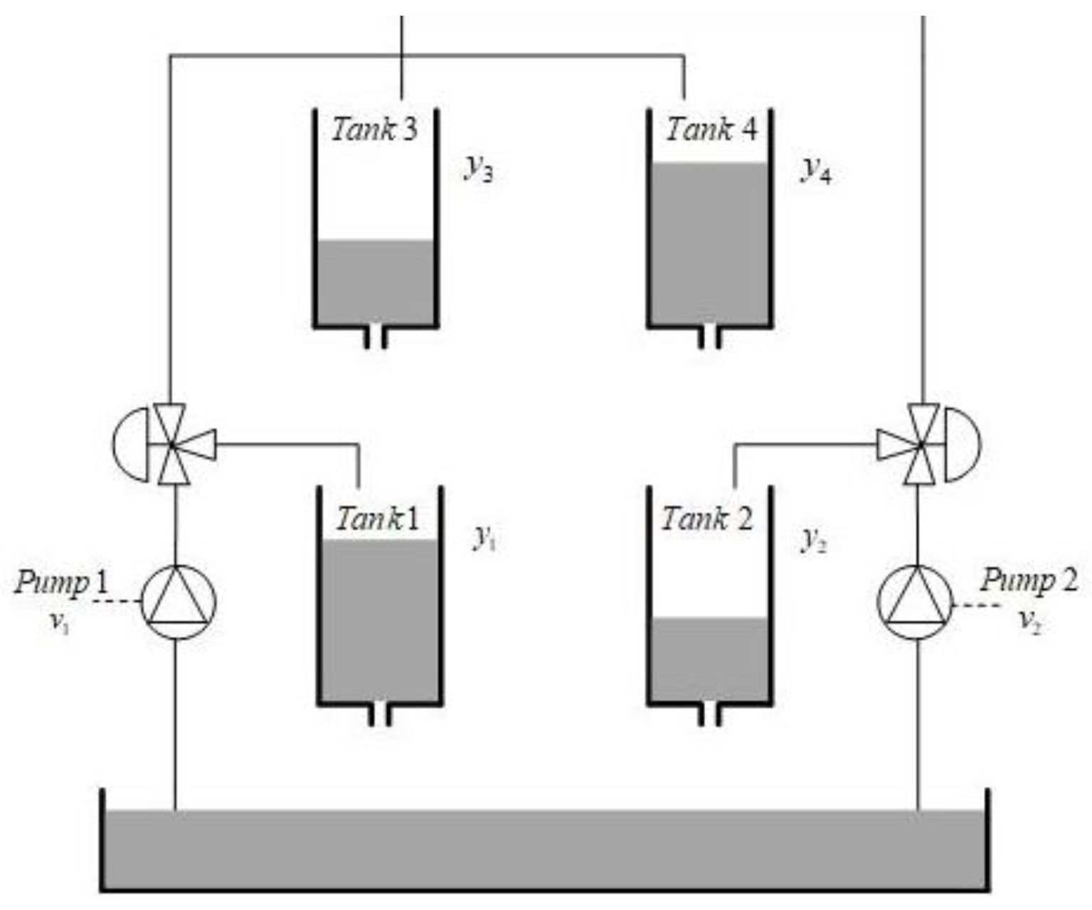
In order to verify the feasibility and effectiveness of the proposed method, simulation experiments were carried out using a model of a quadruple tank [41]. The model consists of four interconnected water tanks and two pumps. The schematic diagram of the quadruple-tank model is shown in Figure 2. In this simulation, represent the variations in the water levels in each of the four tanks, respectively, and the observations of the variation are indicated by , respectively. The inputs are the voltage values to the two pumps that provide water to the four tanks. The model parameters are as follows:
A continuous time-varying fault was applied as follows:
Assume that the actuator-side FDI attack and the sensor-side FDI attack are:
The simulation assumes that the disturbances and noise are independent white noise processes or sequences that obey . We set the initial state , the sampling period , and set .
5.1. The Values of the Correlation Matrices
Using Theorem 1, we set with the help of the Linear Matrix Inequality solver in the LMI toolbox. Then, the robust observer gain matrices and were obtained as follows:
Based on Theorem 2, we set and the security controller gain matrix and the event trigger matrix can also be co-obtained as follows:
5.2. Estimation of System State, FDI Attacks and Actuator Fault
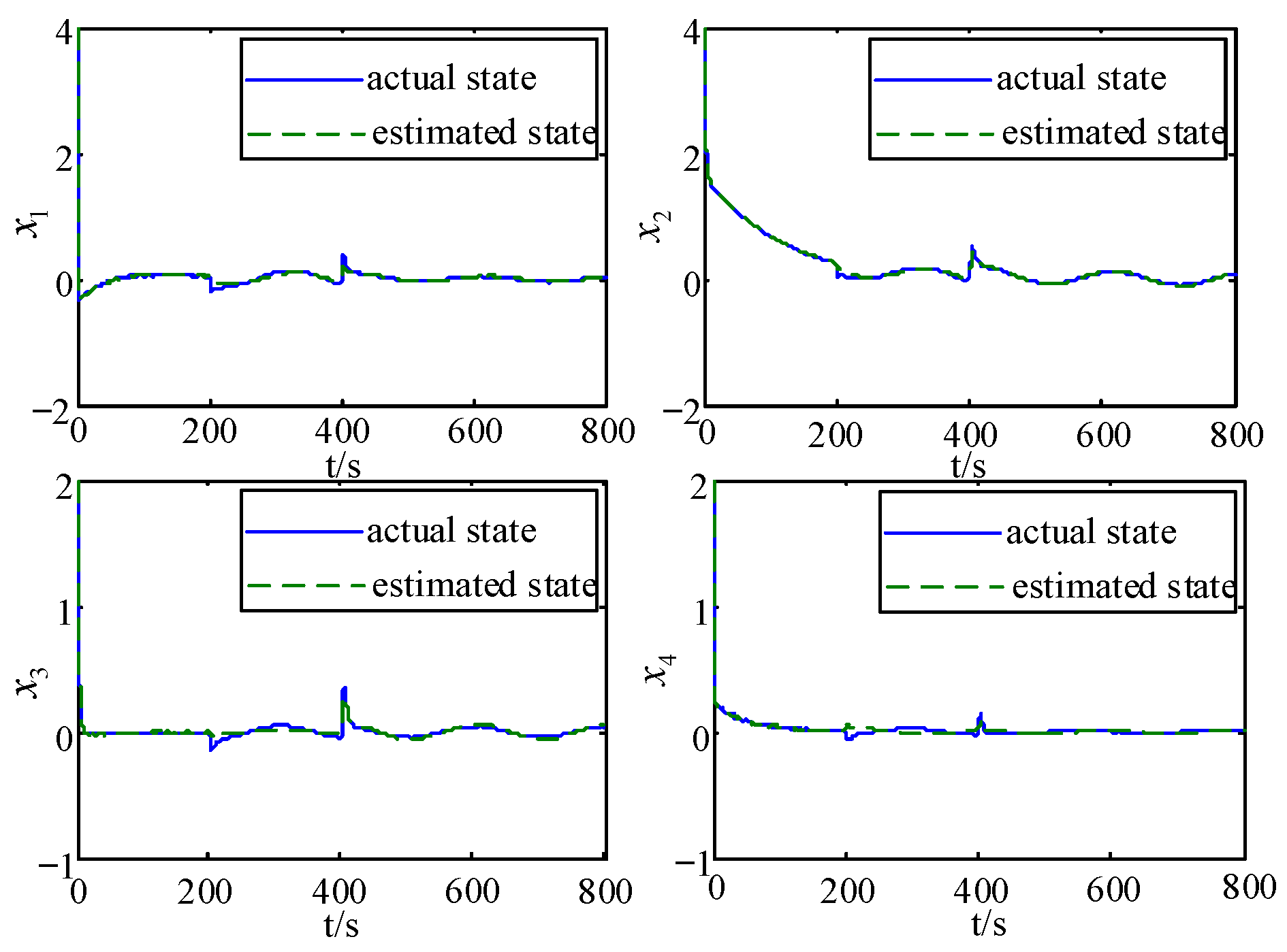
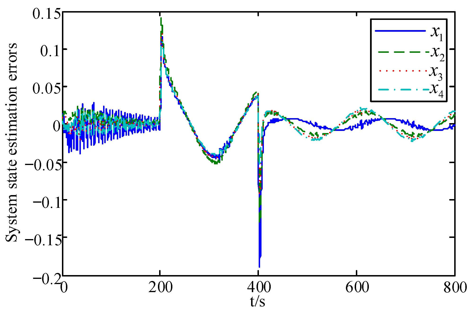
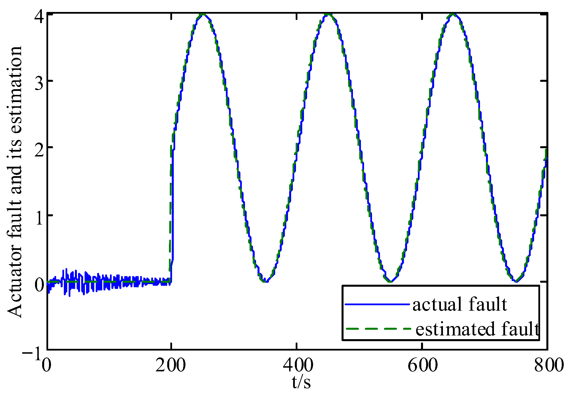
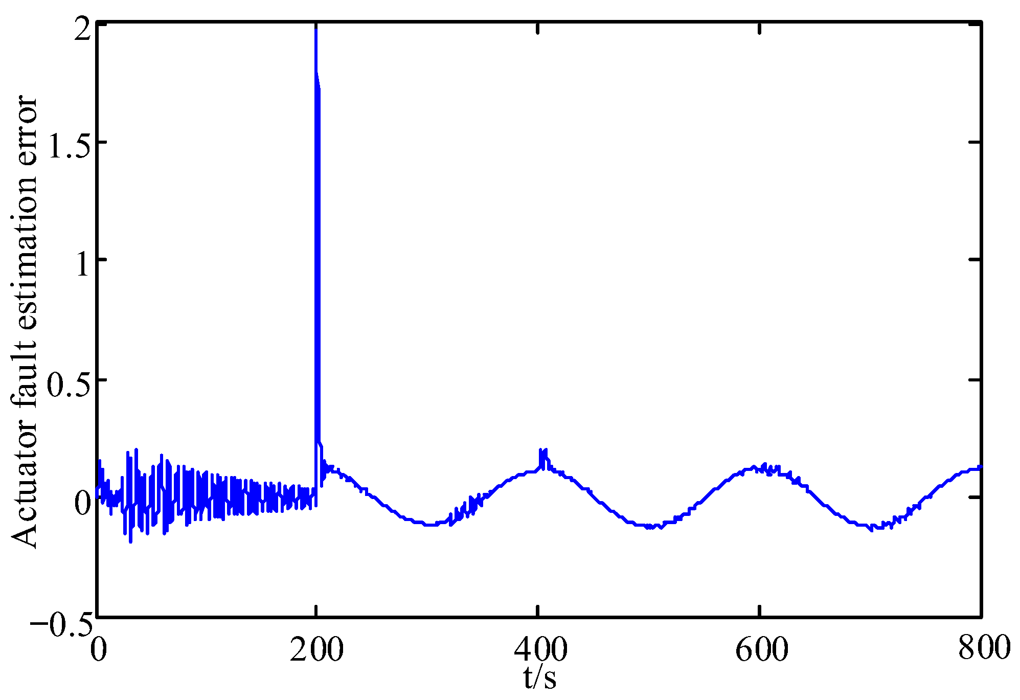
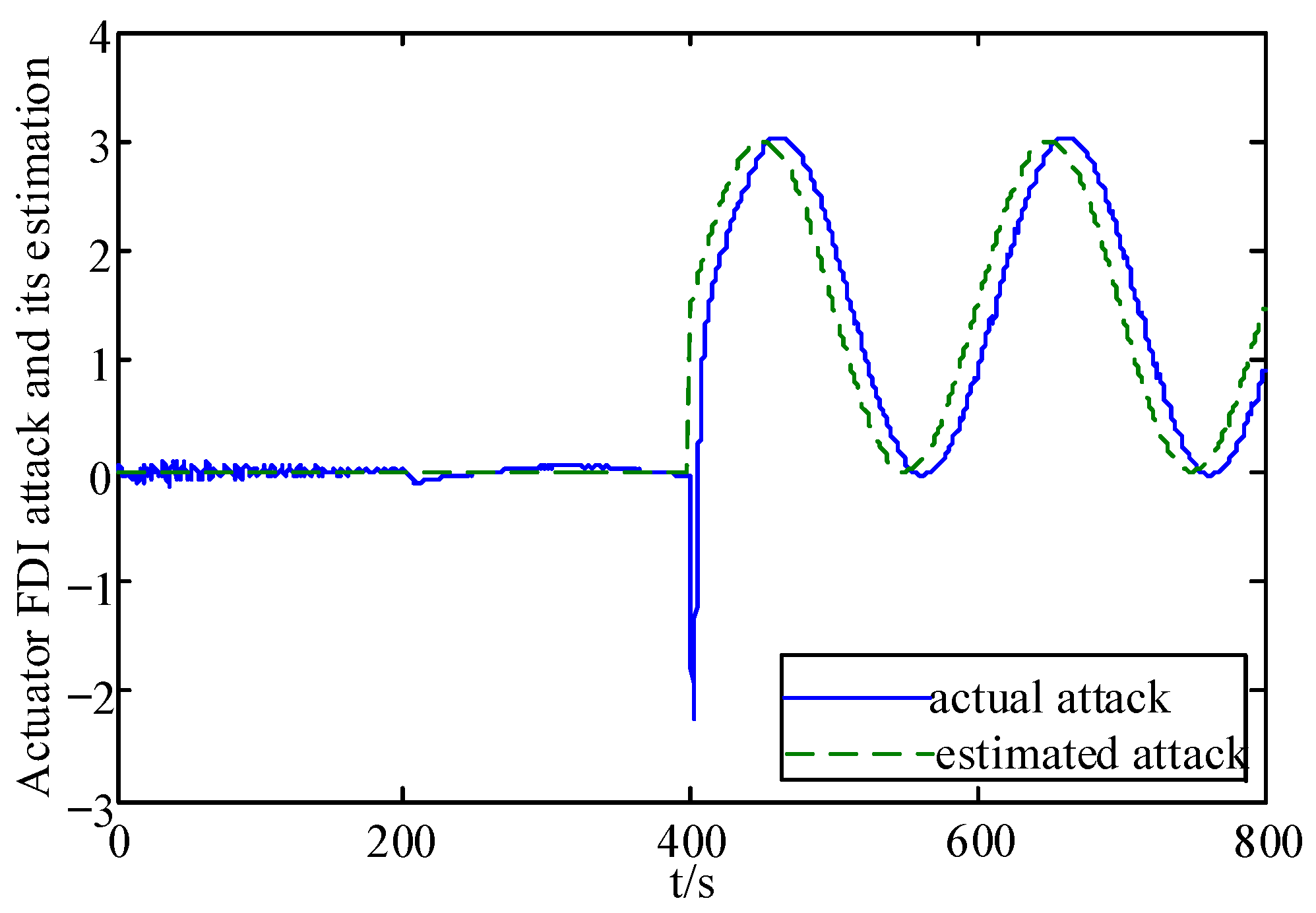
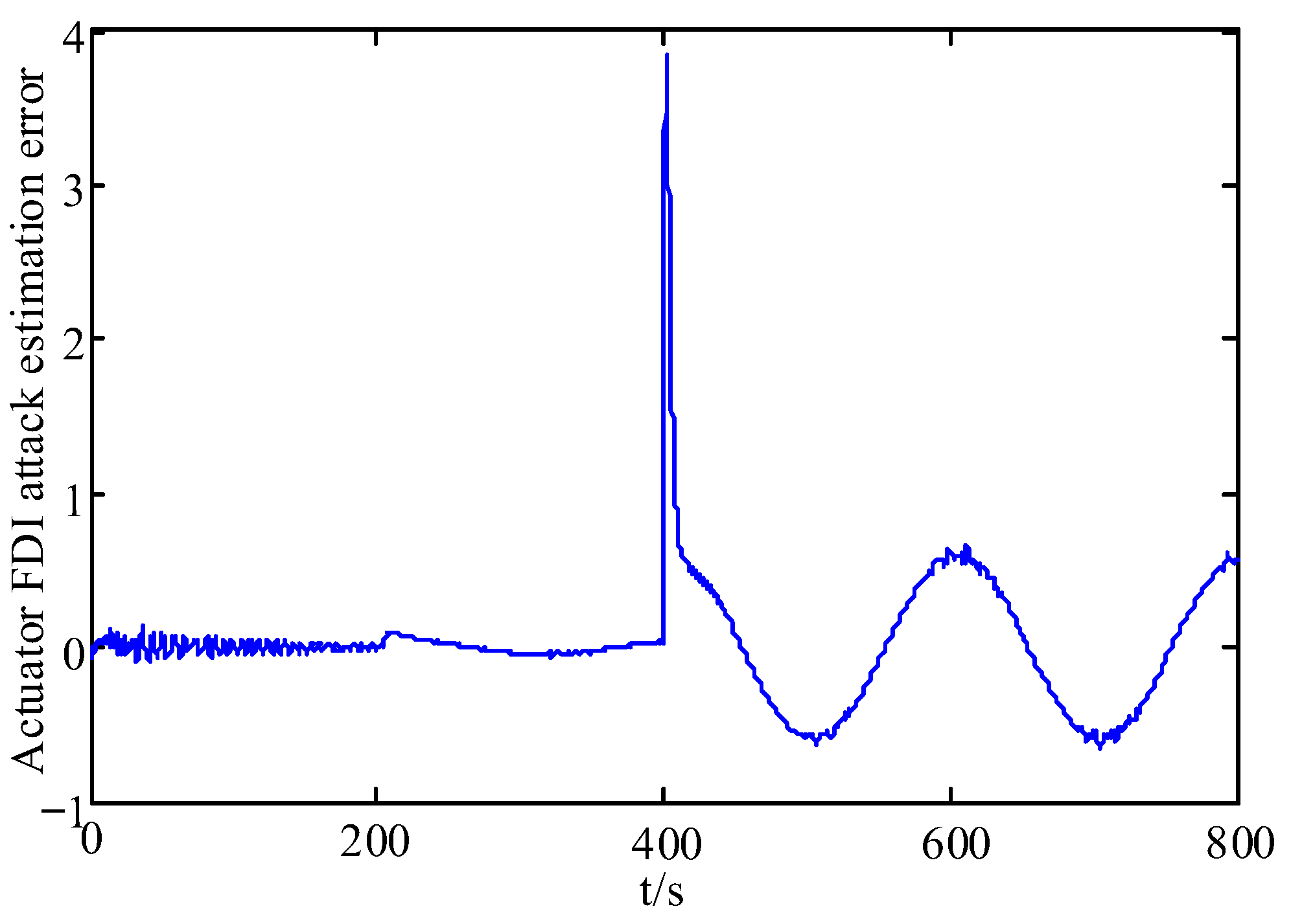
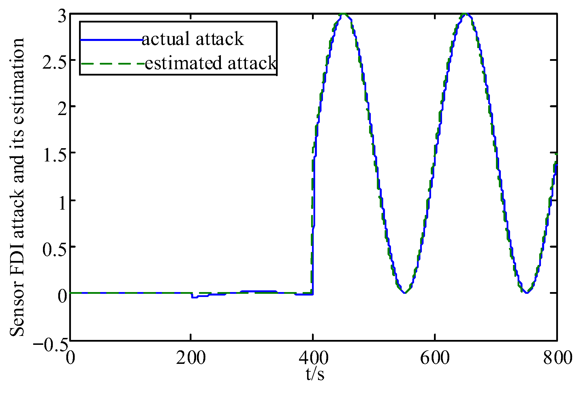
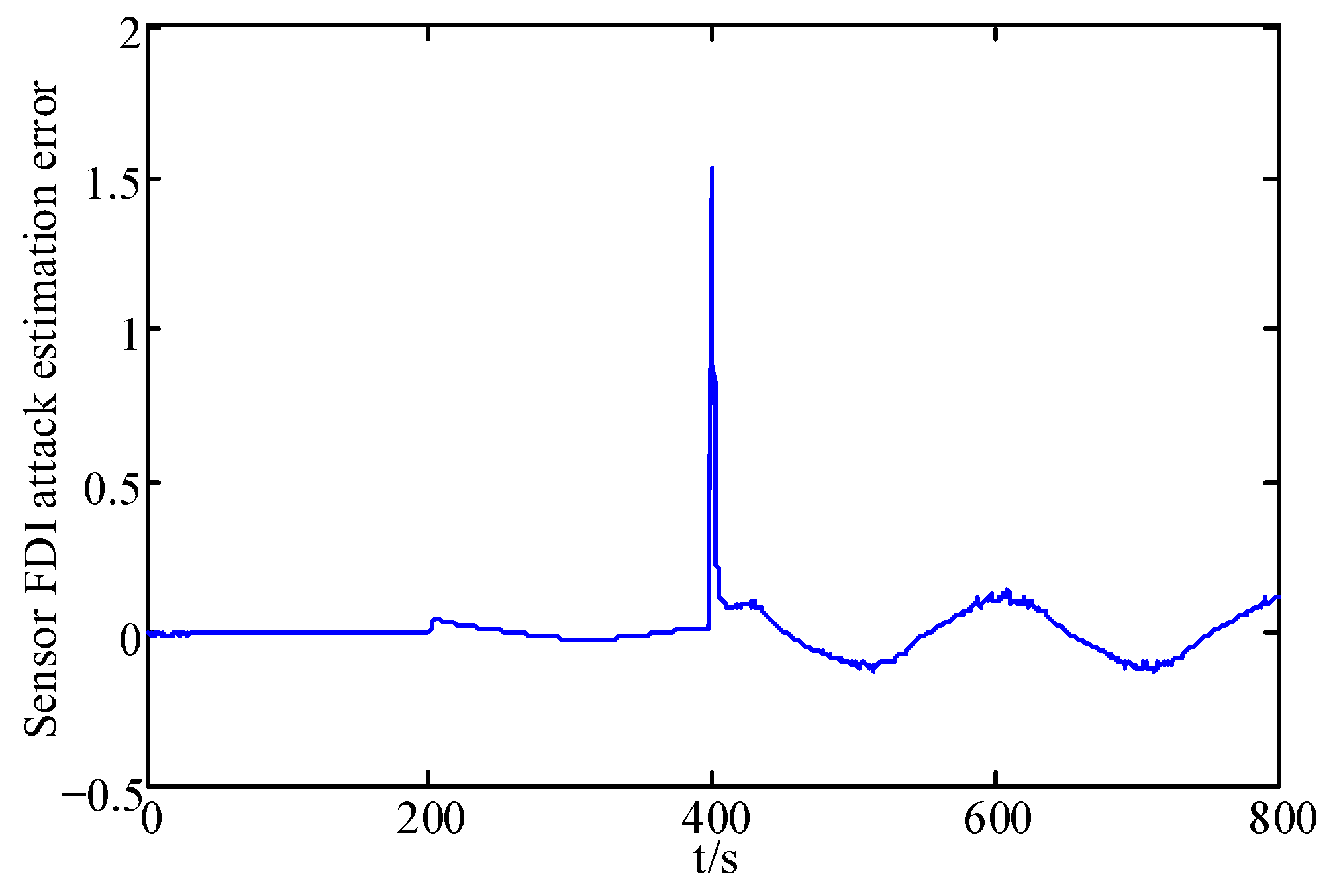
The system states and their estimation; the errors in the state estimation, the fault and its estimation; the error in the fault estimation, the FDI attacks and their estimation; and the errors in the FDI attacks estimation are shown in Figure 3, Figure 4, Figure 5, Figure 6, Figure 7, Figure 8, Figure 9 and Figure 10, respectively.
From these figures, it can be seen that the system state has some fluctuations when FDI attacks and the actuator fault are first added, and remains stable after 500 s, and the system state estimation error only fluctuates between in Figure 3 and Figure 4. In Figure 5 and Figure 6, the actuator fault estimates only fluctuate between . In Figure 7, Figure 8, Figure 9 and Figure 10, the estimation error of the actuator FDI attack fluctuates between , and the sensor side FDI attack fluctuates between . This shows that the augmented observer designed using the method in this paper can estimate the system states, FDI attacks and actuator fault in a timely and accurate way, and that the designed controller is able to keep the system stable quickly under the dual threat of the actuator fault and FDI attacks.
5.3. Comparison and Analysis
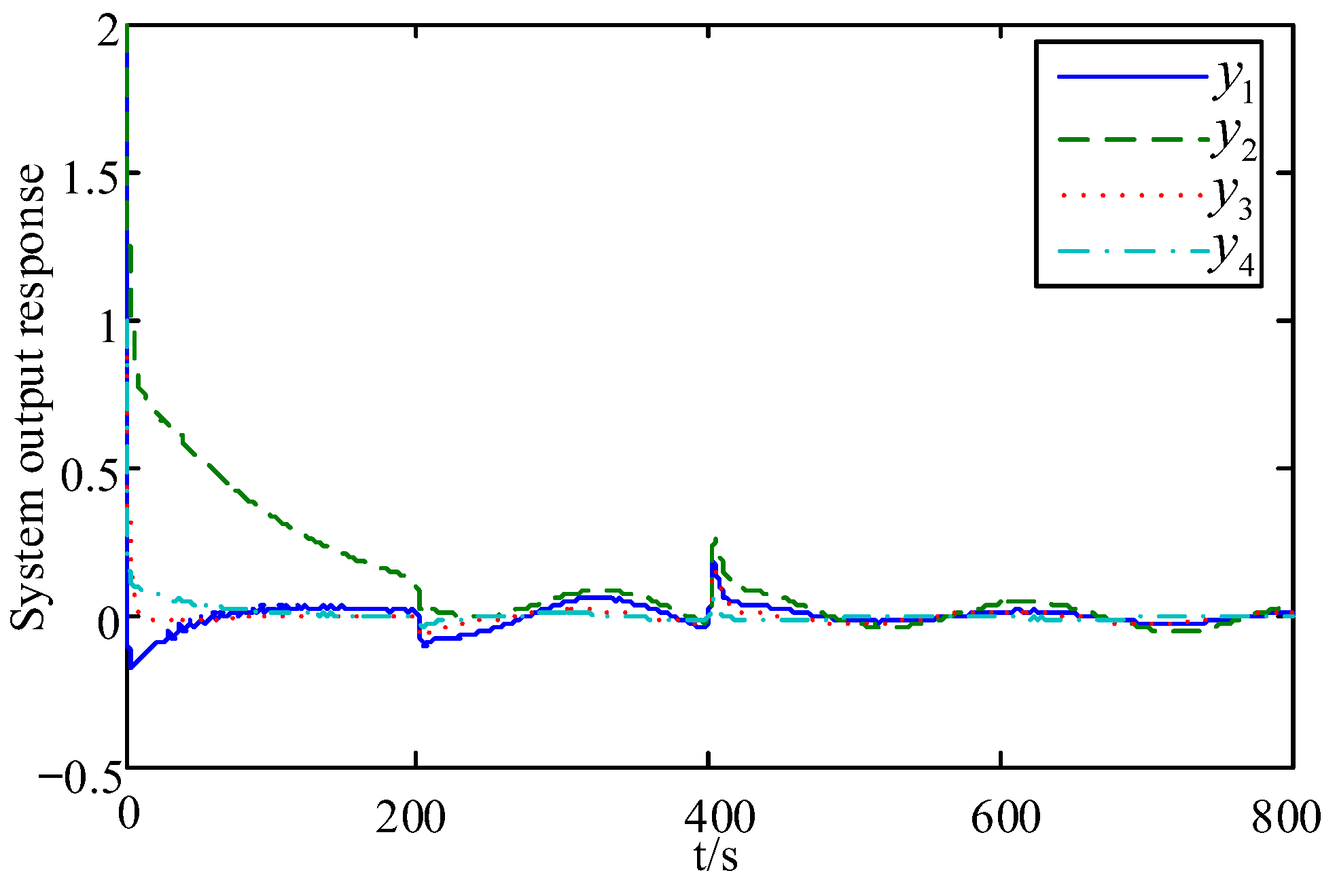
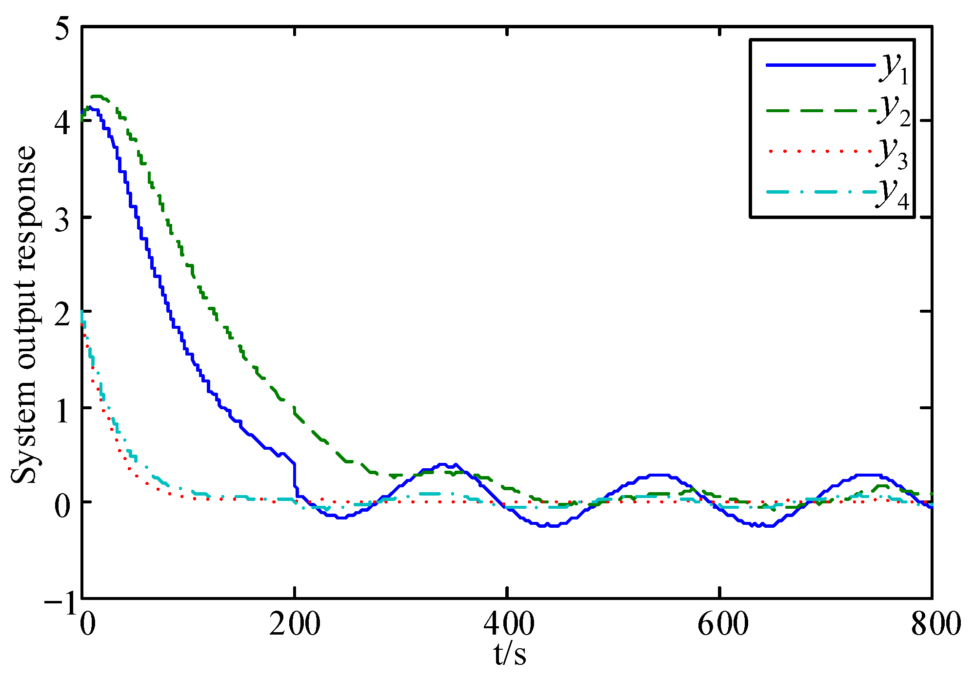
The output response curve of the system when the active attack and fault-tolerant control strategy of this paper is used is given in Figure 11. In order to show the superiority of the active attack-tolerant strategy, the output response curves of the system when using the method in [31] is given in Figure 12 with the same parameters as selected in this paper. The study in [31] still adopted active fault-tolerant control for faults but adopted an active-passive attack-tolerant strategy for FDI attacks (that is, active compensation for actuator FDI attacks and passive tolerance for sensor FDI attack).
Comparing Figure 11 with Figure 12, it can be seen that, from the dynamic performance point of view, the system output decays to the equilibrium position faster when using the method of this paper for the time . From the steady-state performance point of view, the system output eventually stays within the error band when using the method in [31], whereas the system output obtained by the method proposed in this paper eventually stays in the error band. Obviously, the steady-state error of the system output in [31] is relatively larger than that in this paper. Therefore, the integrated security control strategy of active tolerance for FDI attacks on the double-ended network proposed in this paper is more advantageous in improving the system performance, thus giving the CPS a higher level of security control.
Further, Table 1 shows the data transmission amounts under DETCS with different attack tolerance strategies.
In Table 1, n denotes the data transmission volume, denotes the data transmission rate and denotes the average data transmission period. In 800 s, 1125 data need to be transmitted under DETCS with active attack tolerance proposed in this paper, the data transmission rate is 14.1% and the average transmission period is 0.711 s. In contrast, the active–passive attack tolerance strategy proposed in [31] requires the transmission of 1249 data, with a data transmission rate of 15.6% and an average transmission period of 0.641 s. This further reveals that the active attack tolerance strategy is not only more effective than the active–passive attack tolerance method for integrated defence against FDI attacks and actuator faults, but also saves more network communication resources, thus enhancing the compromise between integrated security control and saving communication resources.
6. Conclusions
We investigated the problem of the co-design of integrated security control and communication for a nonlinear CPS experiencing an actuator fault and FDI attacks. Firstly, we proposed a framework for a nonlinear CPS with active fault tolerance and active attack tolerance under DETCS. We then established a closed-loop CPS fault/attacks model. Secondly, using time-delay system theory, the affine Bessel–Legendre inequality and the LMI technique, we derived less conservative design methods for the observer and controller, and achieved the co-design goals of integrated security control and network communication. Finally, a simulation experiment of a quadruple tank was conducted to illustrate that the proposed method can estimate the system states, actuator faults and FDI attacks quickly and accurately. The proposed approach can also save network communication resources while ensuring an excellent performance of the CPS.
The next research direction is using data-driven intelligent algorithms to achieve anomaly detection and the effective identification and separation of attacks and faults in the system, and then combining them with mechanism-based methods.
Author Contributions
Conceptualization, N.H. and N.Z.; methodology, W.L.; software, L.Z. and Y.L.; validation, L.Z., N.H. and N.Z; formal analysis, L.Z. and Y.L.; investigation, L.Z. and W.L.; resources, L.Z., N.H. and N.Z.; data curation, N.H. and N.Z; writing—original draft preparation, L.Z.; writing—review and editing, L.Z.; visualization, L.Z.; supervision, L.Z.; project administration, L.Z.; funding acquisition, L.Z. All authors have read and agreed to the published version of the manuscript.
Funding
This research was funded by the National Natural Science of China grant number 62163022, and Youth Science and Technology Fund of Gansu Province grant numbers 21JR1RM339, 21JR7RM192.
Data Availability Statement
Not applicable.
Conflicts of Interest
The authors declare no conflict of interest.
References
- Zhang, D.; Wang, Q.G.; Feng, G.; Shi, Y.; Vasilakos, A.V. A survey on attack detection, estimation and control of industrial cyber-physical systems. ISA Trans. 2021, 116, 1–16. [Google Scholar] [CrossRef]
- Peng, C.; Sun, H.; Yang, M.; Wang, Y.L. A survey on security communication and control for smart grids under malicious cyber attacks. IEEE Trans. Syst. Man Cybern. Syst. 2019, 49, 1554–1569. [Google Scholar] [CrossRef]
- Ding, D.; Han, Q.L.; Xiang, Y.; Ge, X.; Zhang, X.M. A survey on security control and attack detection for industrial cyber-physical systems. Neurocomputing 2019, 275, 1674–1683. [Google Scholar] [CrossRef]
- Zhang, K.; Keliris, C.; Polycarpou, M.M.; Parisini, T. Discrimination between replay attacks and sensor faults for cyber-physical systems via event-triggered communication. Eur. J. Control. 2021, 62, 47–56. [Google Scholar] [CrossRef]
- Zhao, J.; Wang, X.; Liang, Z.; Li, W.; Wang, X.; Wong, P.K. Adaptive event-based robust passive fault tolerant control for nonlinear lateral stability of autonomous electric vehicles with asynchronous constraints. ISA Trans. 2021, 127, 310–323. [Google Scholar] [CrossRef] [PubMed]
- Wang, X.; Fei, Z.; Wang, Z.; Liu, X. Event-triggered fault estimation and fault-tolerant control for networked control systems. J. Frankl. Inst. 2019, 356, 4420–4441. [Google Scholar] [CrossRef]
- Shang, Y. Resilient group consensus in heterogeneously robust networks with hybrid dynamics. Math. Methods Appl. Sci. 2020, 44, 1456–1469. [Google Scholar] [CrossRef]
- Shang, Y. Resilient tracking consensus over dynamic random graphs: A linear system approach. Eur. J. Appl. Math. 2022, 34, 408–423. [Google Scholar] [CrossRef]
- Shang, Y. Median-Based Resilient Consensus Over Time-Varying Random Networks. IEEE Trans. Circuits Syst. II Express Briefs 2021, 69, 1203–1207. [Google Scholar] [CrossRef]
- Zhang, J.; Zhang, K.; An, Y.; Luo, H.; Yin, S. An Integrated Multitasking Intelligent Bearing Fault Diagnosis Scheme Based on Representation Learning Under Imbalanced Sample Condition. IEEE Trans. Neural Netw. Learn. Syst. 2023, 1–12. [Google Scholar] [CrossRef]
- Zhang, J.; Huang, C.; Chow, M.-Y.; Li, X.; Tian, J.; Luo, H.; Yin, S. A Data-model Interactive Remaining Useful Life Prediction Approach of Lithium-ion Batteries Based on PF-BiGRU-TSAM. IEEE Trans. Ind. Inform. 2023, 1–11. [Google Scholar] [CrossRef]
- Zhang, J.; Li, X.; Tian, J.; Jiang, Y.; Luo, H.; Yin, S. A variational local weighted deep sub-domain adaptation network for remaining useful life prediction facing cross-domain condition. Reliab. Eng. Syst. Saf. 2023, 231, 108986. [Google Scholar] [CrossRef]
- Li, Y.J.; Li, W. Co-design between α/H∞ fault-tolerant control of networked control system and network communication. J. Jilin Univ. (Eng. Technol. Ed.) 2016, 46, 2010–2020. [Google Scholar]
- Qiu, A.; Zhang, J.; Jiang, B.; Gu, J. Event-triggered sampling and fault-tolerant control co-design based on fault diagnosis observer. J. Syst. Eng. Electron. 2018, 29, 176–186. [Google Scholar] [CrossRef]
- Wang, J.; Li, S.Z.; Li, W. Hybrid active-passive robust fault-tolerant control for a networked control system based on an event-triggered scheme. Inf. Control. 2017, 46, 144–152. [Google Scholar]
- Xu, F.; Tan, J.; Wang, X.; Puig, V.; Liang, B.; Yuan, B. Mixed active/passive robust fault detection and isolation using set-theoretic unknown input observers. IEEE Trans. Autom. Sci. Eng. 2017, 15, 863–871. [Google Scholar] [CrossRef]
- Zuo, Z.Q.; Cao, X.; Wang, Y.J. Security control of multi-agent systems under false data injection attacks. Neurocomputing 2020, 404, 240–246. [Google Scholar] [CrossRef]
- Lei, L.; Yang, W.; Yang, C. Event-based distributed state estimation over a WSN with false data injection attack. IFAC Pap. 2016, 49, 286–290. [Google Scholar] [CrossRef]
- Huang, X.; Dong, J.X. A robust dynamic compensation approach for cyber-physical systems against multiple types of actuator attacks. Appl. Math. Comput. 2020, 380, 125–284. [Google Scholar] [CrossRef]
- An, L.W.; Yang, G.H. Improved adaptive resilient control against sensor and actuator attacks. Inf. Sci. 2018, 423, 145–156. [Google Scholar] [CrossRef]
- Sun, Z.; Xue, W.; Liu, J.; Chen, F.; Lu, X. Adaptive event-triggered resilient control of industrial cyber physical systems under asynchronous data injection attack. J. Frankl. Inst. 2022, 359, 3000–3023. [Google Scholar] [CrossRef]
- Chen, C.; Chen, Y.; Zhao, J.; Zhang, K.; Ni, M.; Ren, B. Data-Driven Resilient Automatic Generation Control Against False Data Injection Attacks. IEEE Trans. Ind. Inform. 2021, 17, 8092–8101. [Google Scholar] [CrossRef]
- Tang, B.; Yan, J.; Kay, S.; He, H. Detection of false data injection attacks in smart grid under colored gaussian noise. In Proceedings of the 2016 IEEE Conference on Communications and Network Security (CNS), Philadelphia, PA, USA, 17–19 October 2016; pp. 172–179. [Google Scholar]
- Xiong, X.; Hu, S.; Sun, D.; Hao, S.; Li, H.; Lin, G. Detection of false data injection attack in power information physical system based on SVM-GAB algorithm. Energy Rep. 2022, 8, 1156–1164. [Google Scholar] [CrossRef]
- Pang, Z.H.; Fan, L.Z.; Sun, J.; Liu, K.; Liu, G.P. Detection of stealthy false data injection attacks against networked control systems via active data modification. Inf. Sci. 2021, 546, 192–205. [Google Scholar] [CrossRef]
- Wu, S.; Jiang, Y.; Luo, H.; Zhang, J.; Yin, S.; Kaynak, O. An integrated data-driven scheme for the defense of typical cyber–physical attacks. Reliab. Eng. Syst. Saf. 2022, 220, 108257. [Google Scholar] [CrossRef]
- Hu, L.; Wang, Z.; Han, Q.L.; Liu, X. State estimation under false data injection attacks: Security analysis and system protection. Automatica 2018, 87, 176–183. [Google Scholar] [CrossRef]
- Li, F.F.; Tang, Y. False data injection attack for cyber-physical systems with resource constraint. IEEE Trans. Cybern. 2020, 50, 729–738. [Google Scholar] [CrossRef]
- Ao, W.; Song, Y.; Wen, C.; Lai, J. Finite time attack detection and supervised secure state estimation for CPSs with malicious adversaries. Inf. Sci. 2018, 451–452, 67–82. [Google Scholar] [CrossRef]
- Li, W.; Shi, Y.H.; Li, Y.J. Research on secure control and communication for cyber-physical systems under cyber-attacks. Trans. Inst. Meas. Control. 2019, 41, 3421–3437. [Google Scholar] [CrossRef]
- Zhao, L.; Li, W. Co-design of dual security control and communication for nonlinear CPS under FDI attacks. Meas. Control. 2022, 55, 767–782. [Google Scholar] [CrossRef]
- Yaseen, A.A.; Bayart, M. Cyber-attack detection with fault accommodation based on intelligent generalized predictive control. IFAC Pap. 2017, 50, 2601–2608. [Google Scholar] [CrossRef]
- Li, Y.J.; Wu, Q.E.; Peng, L. Simultaneous event-triggered fault detection and estimation for stochastic systems subject to deception attacks. Sensors 2018, 18, 321. [Google Scholar] [CrossRef]
- Ye, D.; Luo, S.P. A co-design methodology for cyber-physical systems under actuator fault and cyber attack. J. Frankl. Inst. 2019, 356, 1856–1879. [Google Scholar] [CrossRef]
- Peng, C.; Han, Q.-L.; Yue, D. To Transmit or Not to Transmit: A Discrete Event-Triggered Communication Scheme for Networked Takagi–Sugeno Fuzzy Systems. IEEE Trans. Fuzzy Syst. 2012, 21, 164–170. [Google Scholar] [CrossRef]
- Lu, A.Y.; Yang, G.H. Event-triggered secure observer-based control for cyber-physical systems under adversarial attacks. Inf. Sci. 2017, 420, 96–109. [Google Scholar] [CrossRef]
- Xiao, H.Q.; He, Y.; Wu, M.; Xiao, S.P. H∞ output tracking control for sampled-data networked control systems in T-S fuzzy model. Acta Autom. Sin. 2015, 41, 661–668. [Google Scholar]
- Liu, K.; Fridman, E. Wirtinger’s inequality and Lyapunov-based sampled-data stabilization. Automatica 2012, 48, 102–108. [Google Scholar] [CrossRef]
- Lee, W.I.; Lee, S.Y.; Park, P.G. Affine bessel-legendre inequality: Application to stability analysis for systems with time-varying delays. Automatica 2018, 93, 535–539. [Google Scholar] [CrossRef]
- Park, P.G.; Ko, J.W.; Jeong, C. Reciprocally convex approach to stability of systems with time-varying delays. Automatica 2011, 47, 235–238. [Google Scholar] [CrossRef]
- Johansson, H.K. The quadruple-tank process: A multivariable laboratory process with an adjustable zero. IEEE Trans. Control. Syst. Technol. 2000, 8, 456–465. [Google Scholar] [CrossRef]
Figure 1.
Integrated security control framework for nonlinear CPS.

Figure 2.
Schematic diagram of the quadruple-tank model.

Figure 3.
States and their estimation.

Figure 4.
Estimation error of system states.

Figure 5.
Continuous time-varying fault and its estimation.

Figure 6.
Fault estimation error.

Figure 7.
Actuator FDI attack and its estimation.

Figure 8.
Estimation error of the actuator FDI attack.

Figure 9.
Sensor FDI attack and its estimation.

Figure 10.
Estimation errors of the sensor FDI attack.

Figure 11.
System output response curve with active attack tolerance in this paper.

Figure 12.
System output response curve with active–passive attack tolerance in [31].
Figure 12.
System output response curve with active–passive attack tolerance in [31].


Table 1.
Comparison of data transmission in active and active–passive attack tolerance control.
| Methods | n | ||
|---|---|---|---|
| Active attack tolerance in this paper | 1125 | 14.1% | 0.711 s |
| Active–passive attack tolerance in [31] | 1249 | 15.6% | 0.641 s |
Disclaimer/Publisher’s Note: The statements, opinions and data contained in all publications are solely those of the individual author(s) and contributor(s) and not of MDPI and/or the editor(s). MDPI and/or the editor(s) disclaim responsibility for any injury to people or property resulting from any ideas, methods, instructions or products referred to in the content. |
© 2023 by the authors. Licensee MDPI, Basel, Switzerland. This article is an open access article distributed under the terms and conditions of the Creative Commons Attribution (CC BY) license (https://creativecommons.org/licenses/by/4.0/).
Share and Cite
MDPI and ACS Style
Zhao, L.; Li, W.; Li, Y.; Han, N.; Zheng, N. Integrated Security Control for Nonlinear CPS with Actuator Fault and FDI Attack: An Active Attack-Tolerant Approach. Actuators 2023, 12, 216. https://doi.org/10.3390/act12050216
AMA Style
Zhao L, Li W, Li Y, Han N, Zheng N. Integrated Security Control for Nonlinear CPS with Actuator Fault and FDI Attack: An Active Attack-Tolerant Approach. Actuators. 2023; 12(5):216. https://doi.org/10.3390/act12050216
Chicago/Turabian StyleZhao, Li, Wei Li, Yajie Li, Nani Han, and Naiqin Zheng. 2023. "Integrated Security Control for Nonlinear CPS with Actuator Fault and FDI Attack: An Active Attack-Tolerant Approach" Actuators 12, no. 5: 216. https://doi.org/10.3390/act12050216
Note that from the first issue of 2016, this journal uses article numbers instead of page numbers. See further details here.