
Microactuation of Magnetic Nanofluid Enabled by a Pulsatory Rotating Magnetic Field
by
 , , and
Lucian Pîslaru-Dănescu
1,*,
George-Claudiu Zărnescu
1, 
Eros-Alexandru Pătroi
2,
Rareș-Andrei Chihaia
3 and
Gabriela Telipan
1 1
Laboratory of Sensors/Actuators and Energy Harvesting, National Institute for Research and Development in Electrical Engineering ICPE-CA, 030138 Bucharest, Romania
2
Magnetic Materials and Applications Department, National Institute for Research and Development in Electrical Engineering ICPE-CA, 030138 Bucharest, Romania
3
Renewable Sources and Energy Efficiency Department, National Institute for Research and Development in Electrical Engineering ICPE-CA, 030138 Bucharest, Romania
*
Author to whom correspondence should be addressed.
Actuators 2023, 12(5), 210; https://doi.org/10.3390/act12050210
Submission received: 14 March 2023
/
Revised: 12 May 2023
/
Accepted: 16 May 2023
/
Published: 19 May 2023
(This article belongs to the Special Issue Recent Advances in the Design and Applications for Magnetoelastic and Electroelastic Actuators)
Abstract
:A microactuation process was developed with the help of four coils that generate a pulsatory rotating magnetic field. A small actuator stator, which contains a 46 mm acrylonitrile butadiene styrene (ABS) opened box and four coils with E-type ferrite cores, was constructed. Simulations were made for different Duty Cycles, 0.2, 0.5, 0.72 and 0.9, and distances above the E cores, between 0.01 and 6 mm. These simulations determined the magnetic bubble inflating distance, the saturation regions and the average forces that are responsible for nanofluid flow inside the ABS box. An electrical driving scheme was designed, and a drive was constructed to activate four inductive loads that generate a pulsatory rotating magnetic field. The electronic drive can change the actuation frequency (rotation speed) between 1 Hz and 25 Hz and can adjust the Duty Cycle between 5% and 95% (driving force). From simulations and experiments, it was observed that the Duty Cycle must be limited to 0.7 to avoid the magnetic nanofluid saturation at 45 mT. It was found that three applications use a pulsatory rotating magnetic field: a small motor, a small flat pump and a manipulating sheet matrix for displays or chemical droplets mixing.
1. Introduction
Magnetic nanofluid acoustic damping, power compression reduction and voice coil centering technology have been applied for small loudspeakers and large woofers since 2012 [1]. There are several advantages when using the magnetic nanofluid around the loudspeaker coil: sound performance is improved, internal pressure is relieved through venting and coil cooling is achieved.
The thermo-magnetic convection of Mn-Zn magnetic nanofluids was investigated both experimentally and by using simulations. It was observed that there is a self-pumping magnetic cooling effect when an external magnetic field is applied to the fluid [1]. The magnetic field pushes the fluid and acts like a pump without any mechanical moving parts. By using the same principle, a solar Stirling engine can be imagined. This engine can be equipped with pistons realized from magnetic nanofluids, which can also perform as friction seals.
Inertial sensors were developed by using the self-levitation of a magnetic object when immersed in a magnetic nanofluid [2]. The displacement of the levitated mass blocks causes an uneven volume distribution of the magnetic nanofluid in the containers. External positioned coils or Hall elements detect the inductance or magnetic flux change due to magnetic nanofluid displacement. The magnetic nanofluid mass blocks move back and forth, generating the output voltages that are further processed by a differential amplifier circuit.
The results of Ref. [3] aimed to characterize a microrotary motor based on magnetic nanofluid and a rotating magnet, which levitates inside a catheter tube. The flexible stator was made by using a double-sided copper-clad polyimide film. This film was lithographically patterned, and the copper substrate was etched using a dry film of photoresist laminated on both sides [3]. The resulting flexible film was wrapped and bonded on a catheter tube with the driving coils laying on the opposing sides and with a 90-degree positioning angle. The 1.6 mm and 500 μm magnetic shafts levitate and rotate inside the catheter tube with the help of a magnetic nanofluid that acts like a self-sustained liquid bearing. A prism mirror was mounted on the shaft for real-time monitoring and endoscopic optical imaging. The use of magnetic nanofluid enabled further miniaturization of catheter tubes from 2 mm to 0.8 mm.
An experimental microactuator that utilizes a magnetic nanofluid has a dedicated electronic module that implements the pulse width modulation (PWM) principle. The designed actuator was powered with pulses of adjustable frequency 1–250 Hz and a pulse Duty Cycle between 10–90% to control the electrical currents from a set of ferrite-cored coils [4]. By adjusting the currents with short- or long-duration pulse triggers, low currents or high currents were obtained. These pulses were generating motion in the fluid, which was evidenced through stationary surface waves. These surface waves can be used to generate linear or rotational movement.
A microactuation process by using two coils completely immersed in the magnetic nanofluid was described in Ref. [5]. The nanoparticles of Fe3O4 (NPS) were synthetized through the method of coprecipitation. The nanoparticles, with a medium size of 14 nm, were dispersed in a transformer oil, UTR 30 type. The PWM principle was used for the construction of the electronic control system, and these two coils were excited with two rectangular waveforms with a maximum amplitude of 14.5 V, a pulse duty factor of 15% and a 5.809 Hz frequency. These rectangular pulses were processed to be in antiphase. One signal was made the complement of the other one by using two CMOS 4047 integrated circuits; the first one was used as an oscillator, and the second one was used as a monostable with complementary outputs. This driving mechanism can generate useful work; similar to a two-piston Stirling engine, the camshaft is rotated by these up-and-down complementary motions. Here, magnetic pistons surrounded by magnetic nanofluid can be used to generate this motion. The concept of fluidic bearing has been incorporated to support the weight of a rotor or a magnet slider that was used for linear micromotors [6]. An actuation force of 386 μN or greater is obtained by using a rail track that contains a micropatterned array of planar coils; the magnet slider achieved an average velocity of 19 mm/s. A 1.6 mm-sized NdFeB magnet was used for this linear actuation experiment. For finer stepping motions of 7–8 µm, the current transfer region should be between 40 and 100%, and a current-transfer increment of 1% should be applied.
It is obvious that a magnetic micropump can be realized by using a moving magnet near a magnetic nanofluid column [7]. A closed-loop configuration was used for continuous pumping. A circular geometry was chosen to simplify the fabrication process. In this circular channel, the magnetic nanofluid acted as both a valve and a piston. For the valve, the magnetic nanofluid was kept stationary by a fixed magnet, and a rotating magnetic plug served as a piston to drive the other part of the magnetic nanofluid inside the circular channel, pumping the target liquid. This pump only works if the magnetic nanofluid is immiscible with the pumped fluid. Other pumps were made with two serial silicone check valves, and a pulsed flow was initiated due to the periodic motions of a ferrofluidic plug and external NdFeB permanent magnet. The micropump 100 µm channels were manufactured by powder blasting technique, and the pump body was assembled by using several layers of micromachined polymethylmethacrylate (PMMA) [8]. An interesting magnetic nanofluid valve was proposed by mounting a flat coil and a permanent magnet on the top and the bottom side of the test tube, respectively. When there is no current flow in the coil, the fluid is fully attracted to the permanent magnet side, leaving space for the pumping fluid to pass, and the valve is opened. When the coil is activated, the magnetic nanofluid blocks the flow path, and the valve is closed [9]. The same strategy was used in another work to create control valves and a central plunger for actuation. The new plunger was constructed and operated by two vertical upper coils and one bottom horizontal positioned electromagnet [10]. When the upper left coil is activated, the fluid moves to the left; when the upper right coil is activated, the fluid moves to the right, and for the third state, the plunger is opened. For magnetic nanofluid valves, only two coils were used, one vertical upper coil and one bottom horizontal electromagnet. The magnetic nanofluid was injected into a 4 mm diameter tube with a length of 10 cm.
Few papers made use of rotating magnetic fields to produce motion. Inventor Shaun Detloff applied for a patent in 2013 for a magnetic nanofluid electric motor with rotating magnetic fields [11]. In response to the changing magnetic fields generated by electromagnets, a turbine was rotated by the flow of the magnetic fluid. The rotating magnetic field was induced by three electromagnets arranged in a sliced pancake configuration.
Observations were made to see the magnetic nanofluid flow in a uniform rotating magnetic field produced by a spherical cavity [12]. The spherical cavity consists of two spherical fluxball coils fixed to generate a magnetic field along the x- or y-axis; therefore, the fluxball generates a magnetic field that rotates about the vertical z-axis. The magnetic fluid velocities were measured for different magnetic fields 5, 7.5, 8.75 and 10 mT. The corresponding measured average speed following the previous order was 0.75, 1.2, 1.6 and 2 mm/s. A cylindrical container with magnetic fluid was fixed to the center of the fluxball and with the cylinder axis placed exactly on the z-axis. The magnetic field had a 95 Hz fixed frequency, and the current was increased in steps of 0.25 A. The coils were excited with 90° out-of-phase currents.
Although Shaun Detloff’s patent, registered in 2015 [11], describes a turbine rotated by the flow of the magnetic nanofluid, no force, no pressure interval and no physical dimensions are mentioned there. From his description, the reader can imagine big turbines rotated by the magnetic nanofluid flow, but in reality, this process can be applied only for small turbines (in our case, less than 20 g) due to a low 45 mT material saturation point.
A small actuator stator, composed of a 46 mm acrylonitrile butadiene styrene (ABS) opened box and four coils with E-type ferrite cores, was constructed. A magnetic nanofluid that saturates at 45 mT is located inside this box. An electrical driving scheme was designed, and the drive was constructed to activate four inductive loads that are used to generate a pulsatory rotating magnetic field. The electronic drive can change the actuation frequency between 1 Hz and 25 Hz and can adjust the Duty Cycle between 5% and 95%. The simulations and experiments showed that the Duty Cycle must be limited to 0.7 to avoid the magnetic nanofluid saturation at 45 mT.
It has been observed from experiments that a higher actuation frequency increases the rotational magnetic nanofluid speed, and the Duty Cycle adjusts the current and magnetic field strength to obtain higher magnetic fluid pushing forces. The Duty Cycle and frequency control were used for the actuator stator part. This microactuation process can be applied for at least three applications: a small motor, a small flat pump and to develop a manipulating sheet matrix for displays or chemical droplets mixing.
Here, the authors propose a microactuation process enabled by four coils that generate a pulsatory rotating magnetic field. The paper starts with magnetic nanofluid synthesis and characterization. The magnetization curve is interpolated, and then the magnetic field variation with magnetic field intensity is introduced in simulations. These simulations were made for four different Duty Cycles 0.2, 0.5, 0.72 and 0.9. Moreover, the magnetic field was extracted for a wide distance range between 0.01 and 6 mm to observe the saturation regions and to determine the magnetic nanofluid bubble inflation range. From these simulations, average forces and pressures were estimated; these are responsible for magnetic nanofluid translation from one stator part to another.
2. Materials and Methods
2.1. Magnetic Field Simulations
The magnetic field was modeled for the magnetic nanofluid, depending on the Duty Cycle Da and different flux path distances, considered above the two E cores and inside the magnetic nanofluid rectangle. Here, Duty Cycle Da is dimensionless and represents the ratio between the power transistor conduction time and oscillation period . is the power transistor off time or the time when the current passes through the diode. Oscillation period can be determined from a frequency interval of 0.5…25 Hz. The magnetic nanofluid was represented for three different geometries, as a 3 × 42 mm, 4 × 42 mm and 6 × 42 mm rectangle that is situated above the two E cores. Of course, these geometrical configurations are valid only when the magnetic nanofluid is not moving or when each configuration can be assimilated as a single frame (in time) that is only a part of the whole magnetic nanofluid movement (see Figure 1 and Figure 2).
It can be seen below that the Duty Cycle has a major influence on the average voltage and current and can directly control the magnetic field amplitude and the magnetic pushing force. One geometrical configuration was considered in FEMM for ferrites: two E cores aligned on the entire 42 mm inner box space length and separated by a 2 mm spacer.
The second E core was added because it registered a small additional influence on the magnetic field amplitude and on magnetic nanofluid behavior. Almost no influence was observed when the oscillating frequency was changed from 0 Hz to 3 Hz. Therefore, it cannot be distinguished between a DC power supply and an AC power source at very low frequencies (<3 Hz). It is important to consider a variable thickness between 2 and 6 mm for the magnetic nanofluid and to compare each result to identify where the magnetic field stops changing. The magnetic nanofluid characteristics are described in Appendix A. Moreover, the magnetic nanofluid synthesis, coprecipitation method, treatment with oleic acid (as surfactant) and the final mixture with transformer oil (as stabilizing and carrier agent) are presented in Appendix A. The magnetic nanofluid MH curve Equation (A6), shown in Appendix A, was approximated from the vibrating magnetometer experimental values of magnetization. Then, these values were converted from A/m to T, resulting in JH and BH interpolation curves.
The magnetic nanofluid BH curve was introduced in FEMM 4.2 material library. For 0.0018 T, the magnetic field intensity was 1 kA/m; for 0.0148 T, it was 4 kA/m; for 27 mT, it was 10 kA/m; for 45 mT, 20 kA/m; for 90 mT, 50 kA/m; for 124 mT, 75 kA/m; for 211 mT, 140 kA/m; for 289 mT, 200 kA/m; and for 417 mT, it was 300 kA/m. From 475 kA/m, the magnetic field increased very slowly to 0.640 T, and when starting from 500 kA/m, the magnetic field remained almost constant at 0.67–0.685 T. The saturation magnetization of the magnetic nanofluid is present here at over 500 kA/m for a measured magnetic field of 0.67–0.685 T. From the above simulations (see Figure 2a and Table 1) the highest magnetic field of 45 mT is situated in the vicinity of the coil, at the center and near ferrite edges. Just above the ferrite cores from 0.01 to 0.5 mm distance, inside the magnetic nanofluid and for Da = 0.9 Duty Cycle, the magnetic nanofluid reaches the saturation magnetization of 45 mT. The magnetic field decreases as the viewer moves further away from the ferrites, down to 30 mT, at a 1.5 mm distance.
The maximum magnetic field inside the magnetic nanofluid approaches 44 mT (the scientific notation 4.4e-002 is same as 4.4 × 10⁻²) for 0.72 Duty Cycle and at 0.01 mm distance from E ferrite cores (see Figure 2b). At a 0.5 mm distance and at the same Duty Cycle, the magnetic field is 40 mT. The saturation magnetization can only be avoided from 0.7 Duty Cycle down to 0.2 Duty Cycle.
When one E core electromagnet is activated, the magnetic field encloses, such as in simulations, and the magnetic nanofluid inflates and follows the magnetic field lines. The straight line and rectangular geometry of magnetic nanofluid is only an approximation but can give fast and good results. All simulations were made by using Dirichlet boundary conditions. Seven small boundary layers were used to obtain precise results.
An estimation of the average current passing through the coils and the electronic power scheme is described in Appendix B.
By replacing and , from Equations (A12) and (A13) (Appendix B), inside Equations (A10) and (A11) respectively, Equation (A14) can be rearranged. Equation (1), the final expression for the average current, is obtained by simplifying the exponential terms from Equation (A14).
The calculated average current that depends on the Duty Cycle value and that was also introduced in the simulation is:
Please note that is an arbitrary time that contains all previous periods or cycles k (for a single cycle k = 1), and is the inductive load time constant. If this constant is too big, the current will not have time to rise completely for the given oscillation period, . In our case, , so all exponential terms can be ignored, .
It can be observed that this formula was extracted after calculating the current when the transistor is in conduction mode (On) and in (Off) position. In (Off) position, the current passing through the diode is equal to the inductive load current. It is important to see that the average current was obtained by integrating and summing , the current passing through the transistor in conduction mode, with , which is exactly the load and diode current when the voltage supply is cut off. Without applying integration for [tk…tk + DaTosc] on conduction state interval or off state [tk + DaTosc…tk + Tosc] interval, the average voltage or Da Duty Cycle will be ignored.
The average current (see Equations (A14) and (1) for different Duty Cycles) was obtained by considering the resistance and inductance of the coil, 309 Ω and 0.127 H, respectively. From this given initial data, the load time constant can be extracted, which was much lower than the pulses’ oscillation period .
In the experimental section, a peak voltage of U = 15 V from the rectangular pulse was applied to the coil. In simulations, an average or RMS (root mean square) current must be used to activate the coil.
The voltage and current can be changed by modifying the Duty Cycle to be between 5 and 95%. Depending on how much the transistors were in conduction mode, the pulse was longer in duration, and the average voltage had increased proportionally.
The magnetic field situated at 0.5 mm above E cores was presented in Figure 3a,b, for Da = 0.9 Duty Cycle and Da = 0.72 Duty Cycle. The maximum magnetic field at 0.5 mm distance (Da = 0.9, 2 mm thick magnetic nanofluid) from ferrites increases from 0.04 T, as seen in Figure 3a, up to 0.044 T at 0.5 mm distance (Da = 0.9, 6 mm thick magnetic nanofluid) (see Table 1). The magnetic field remains at the same value of 0.044 T between 4 mm and 6 mm magnetic nanofluid thickness, which means that no additional magnetic nanofluid is needed above the E cores. The 4 mm magnetic nanofluid thickness is the optimum inflation limit.
Moreover, the magnetic field at 0.5 mm above E ferrite cores and inside the magnetic nanofluid is shown in Figure 4. These magnetic field values were also introduced in Table 1 (for Da = 0.2). Ins Table 1, all magnetic field values at different distances above E cores and for selected Duty Cycles (Da), 0.2, 0.5, 0.72 and 0.9, are presented.
If the Duty Cycle is decreased to be under 0.2, the magnetic field amplitude will decrease under 10 mT, and the magnetic nanofluid will no longer inflate, or the inflation will not be visible (see Figure 4a,b). An optimum magnetic nanofluid control will be realized if the Duty Cycle is adjusted between . For the average current is 10 mA. For , the maximum recommended value used in simulations, the average current is 35 mA, and the magnetic field will not increase above 27 mT. If the average current will increase to 44–48 mA, and the magnetic field will exceed 44 mT.
The magnetic nanofluid was simulated by the BH hysteresis curve that is rising up to the saturation point of 0.045 T. From the simulations, it can be seen that the magnetic field inside the magnetic nanofluid is very close to 44–45 mT, under 0.5 mm distance above the core and for . To avoid the saturation point of the magnetic nanofluid, the Duty Cycle can be limited electronically, not to exceed the maximum 0.7 value.
The optimum magnetic nanofluid control can be realized between 0.5 and 0.7 Duty Cycle (see Figure 5 and Figure 6). The Fe-Ni-Zn-V ferrite core type has a magnetization curve that grows from 68 mT and 44 A/m, 0.2 T and 150 A/m, 0.31 T and 1359 A/m, 0.48 T and 63 kA/m, and 0.67 T and 197 kA/m and starts to saturate at 0.83 T and 324 kA/m.
If the values of the magnetic field distribution along the two ferrite cores, for Da = 0.5 (Figure 7), are compared with the obtained magnetic field density for two E ferrite cores at Da = 0.72 (see Figure 8), it can be seen that the magnetic field induction has changed from 15 to 17 mT (at 3–4 mm distance), up to 23–25 mT.
The magnetic field along ferrites, at 1 mm distance above E cores, reaches 22 mT for Da = 0.5 and 30 mT for Da = 0.72 (see Figure 8 and Figure 9). The magnetic field at the first E core center drops down to 5 mT. Moreover, the magnetic field near the secondary E core is very small, about 2 mT. These observations bring us to the conclusion that the secondary E core with no active coil has little influence on the magnetic field path and also on the magnetic nanofluid present above the secondary non-acting core. As it can be seen later from the magnetic nanofluid actuation process, although the magnetic field lines are mainly surrounding the active coil and the E core, forming a magnetic nanofluid dome, the other three non-acting E cores are still keeping a part of the magnetic nanofluid upwards, but at a much lower height. This time, as it can be observed in the density plots, the magnetic nanofluid stays near the edges of the acting E core, where the magnetic field is bigger. In the active E core center, the magnetic field is low, under 5 mT, and is forming a hole.
At 3.5 mm above the E cores (Figure 8), the magnetic field remains near 20 mT. This is also the real limit to where the magnetic nanofluid bubble is rising. The magnetic fluid will rise and form a hemisphere around the active coil until the force of gravity is equilibrated by the magnetic force.
The magnetic field falls below 2 mT when the observer is looking further away from the second non-active coil and E core center. The previous simulations were able to give important information about magnetic field variation with distance considered above the E core (where the magnetic nanofluid is situated), magnetic nanofluid thickness, average current and Duty Cycle.
The magnetic field was investigated for at least four cases, where the Duty Cycle was 0.2, 0.5, 0.72 and 0.9. From these simulations, it can be concluded that is the optimum working interval. Frequency has little or no effect on current because and the magnetic nanofluid will not inflate over 4 mm because the magnetic field amplitude will remain the same at 3.5–4 mm, 0.02 T (), no matter whether the magnetic nanofluid thickness is 4, 6 or 10 mm. The magnetic field amplitude will only start to increase a little over 25 mT when the magnetic nanofluid thickness is 3 mm.
For a maximum of 44–48 mA current, the magnetic nanofluid will be in the saturation region.
2.2. Electronic Drive Circuit
The main role of the electronic drive circuit is to ensure precise control of magnetic field intensity and induction produced by each of the four coils. These four coils, L1, L2, L3 and L4, are activated by rectangular pulse trains, such as in Figure 9a,b.
The first CD4047 oscillator generates a rectangular Vosc voltage signal with a frequency between 4 and 100 Hz. As the CD4047 oscillator is set as an astable multivibrator τosc = 4.4 R1 C1, the variable resistance limits must be calculated accordingly to Equations (2)–(4). The C1 has a fixed capacitance value of 100 nF. It results in fmax = 100 Hz and fmin = 4 Hz.
However, if and C1 = 100 nF, it can be determined that R10 = 22.7 kΩ and = 528 kΩ. A 500 kΩ potentiometer must be chosen and connected in series with a 20 or 22 kΩ fixed resistor and one 100 nF capacitor to adjust the oscillator frequency to be between 4.3 and 113 Hz (see Equations (2)–(4)).
A 74HC4017D or CD4017 Johnson decade counter with internal flip-flops logic circuits was used to create the train of four pulses, with the timing presented in the datasheet and as seen in previous pictures. The timing pulse sequence of the first Q1 flip-flop logic gate was followed by the secondary pulse sequence of the Q2 flip-flop gate until all Q1…Q9 carry-out signals formed a decade sequence. From this sequence, only four signals, Q1, Q2, Q3 and Q4, were chosen to be useful signals for the 4066 digital switching circuit and to control L1, L2, L3 and L4 coils. As can be noticed in the datasheet, the decade counter takes the clock signal frequency given by the CD 4047 oscillator and decreases it by two times for each flip-flop gate. Moreover, each CD4047 chip has an internal frequency divider (by 2) for both astable and monostable modes. If the signals from pin 10 are used for the output of the oscillator, it should be taken into account that the oscillator frequency will be divided by 4 and will be applied to the transistor gates by using channels 1…4. Power transistors switch on and off at a pulsed repetition frequency situated between 0.5 and 25 Hz, initiating or interrupting the power supply for each coil according to the previous timing sequence.
While the oscillator is generating and sending a VOSC signal at the Johnson clock terminal, the same Vosc signal is reformed by two series inverting NAND (4011 chip) or NOT (4041) logic gates and applied to the triggering entrance of a monostable CD4047 chip. This integrated circuit arranged in a monostable configuration is used for modifying the Duty Cycle factor between 5 and 95%. This monostable circuit allows the pulses to pass only in the selected positive edge signal window, established by the Duty Cycle factor and monostable τmon = 2.48 R2 C6 triggering time.
If C6 capacitance is set to 100 nF, the variable R*2 potentiometer value limits can be calculated.
The Duty Cycle Da has an adjusting interval between 5% and 95%. If the minimum Duty Cycle Damin = 5% and the maximum fmax = 100 Hz oscillator frequency, we should be able to determine the variable resistance R2 lower limit. The potentiometer R*2 minimum value will be:
If the maximum Duty Cycle is chosen to be 95% and the minimum fmin = 4 Hz oscillator frequency, the variable resistance R2 higher limit can be determined. The maximum value of the potentiometer will be:
Equations (5)–(8) resulted in R2min = 2…50 kΩ and R2max = 957 kΩ; these are the variable resistance limits that are necessary to keep the Duty Cycle inside 5–95% interval for frequencies variating between 4 and 100 Hz. Overall, a 1 MΩ variable potentiometer was needed to cover the entire Duty Cycle range.
If R20 = 47 kΩ is selected to be a minimum series resistance in order to keep the Duty Cycle inside a 5% lower limit, for 4 Hz frequencies, it will be impossible to set the Duty Cycle to be 5% for higher frequencies, such as at 100 Hz. Moreover, if R20 = 1.8 kΩ, the Duty Cycle can be set to a minimum of 0.18% at 4 Hz. The Duty Cycle can now be set to 5% at 100 Hz.
From Equation (9), it can be concluded that .
The load of IGBT transistors is represented by the inductance coils L1, L2,…,L4. Thus, the coils can be controlled using a rectangular voltage with variable “f” frequency in the range of 1 Hz ÷ 25 Hz.
At the exit pins of each digital switch from the 4066 chip, a train of rectangular pulses U1, U2,…, U4 is obtained, such as in Figure 10 and Figure 11. These train pulses are used to control the power IGBT groups (Q5, Q6), (Q11, Q12), (Q17, Q18) and (Q23, Q24). Each group of two power transistors has a buffer circuit where the gates are connected. The buffer consists of one 2N1711 NPN transistor; two BD139, BD 140, NPN and PNP transistors pair arranged in series connection; and one smaller G7N60C3D IGBT rated at 600 V and 14 A to bring the gate to the ground and disconnect the group of power IGBT’s. The buffer acts depending on the channel’s signals; when the channel signal is on or HIGH, the 2N1711 transistor brings the gates of these two BD139 and BD140 complementary transistors to the ground. The BD140 PNP transistor switches on, and BD139 switches off, meaning that the G7N60C3D IGBT gate will also be connected to the ground, and the G7N60C3D IGBT will be turned off. In this case, the gates of the power IGBT’s pair stay positive, and the corresponding coil is supplied with current.
When the channel signal is LOW, the 2N1711 transistor keeps the gates of these two BD139 and BD140 complementary transistors to the positive side. The BD140 PNP transistor switches off, and the BD139 NPN transistor switches on, meaning that the G7N60C3D IGBT gate will also be connected to the positive side, and the G7N60C3D IGBT will be turned on, bringing the power IGBT gates to the ground. In this case, the power IGBT pair will be turned off, and no current will pass through the corresponding coil.
Each buffer will act similarly to allow or block the current flowing path from the 15 V voltage source.
In Figure 10 and Figure 11, the electronic scheme is presented for controlling coils L1, L2, L3 and L4. The inductive kick overvoltage can be 3 to 4 times higher than the supply voltage. In our case, the activating pulse frequency is small, 1–25 Hz, so only a high inductance could cause a rapid voltage spike. The coil’s inductances with the E ferrite cores were measured at different frequencies between 20 and 100 Hz, and all four inductances were 0.126–0.127 H. The electronic power scheme is described in Appendix B.
2.3. Actuator Fabrication and Experiments
An ABS box was 3D printed to be used as a support for both E-type ferrite cores and to retain the magnetic fluid (see Figure 1). This box is composed of four equal squared compartments 20 mm in length. The 3D-printed wall has a thickness of 2 mm. E-type ferrite cores also have the same length of 20 mm, and each central leg has a squared surface of 5 × 5 mm2. Each lateral leg has a surface of 5 × 3.5 mm2. The overall ferrite height is 10 mm, and the space between legs is 4 mm. This space was used to mount the coils. Each coil support has a 6 mm squared hole to be suited to the leg surface, and the useful winding surface is 4 × 6 mm2. The coil support has a height of 6 mm. The coil winding wire had a diameter of 0.06 mm, and the coil had a number of 1534 turns. The same 2 mm wall thickness was used as a spacer in simulations. The inner box height was 16 mm to let the magnetic nanofluid be poured a little above the coils and E ferrite cores and to have space to observe the magnetic nanofluid 3–4 mm inflation without spilling the fluid across the outside walls. Any E-type soft ferrite with a total flux path length of 20 mm could be used, but the recommended core materials for lower than 200 kHz frequencies are 3C81, 3C90…93.
The laboratory equipment used for magnetic fluid experiments was the following:
- -
- Agilent E4980 A LCR Meter;
- -
- Keysight 53210 A RF Counter;
- -
- FLUKE 281 40 Ms/s Arbitrary Waveform Generator;
- -
- Agilent 34461 A 6 ½ Digit Multimeter;
- -
- Tektronix TDS 2014 B Digital Storage Oscilloscope;
- -
- NI LabVIEW Signal Express Tektronix Edition;
- -
- AC/DC Current Probe FLUKE 80i-110s, Sensitivity 100 mV/A.
Measurements were made at room temperature (22 ± 3 °C) and humidity of 48.2 RH.
Coil inductance measurements from Table 2 were made with Agilent E4980 A LCR Meter at different frequencies. Because this actuator is controlled at frequencies below 20 Hz, the coil inductance has little influence on series impedance Z. The coil resistance with 309 Ω and the 15 V coil average supply voltage values were used for current estimation and as an input parameter in previous simulations. It is known that frequency, total 1534 number of turns and average current must be introduced in FEMM 4.2 as input parameters, besides the soft magnetic materials and copper strands selection.
As the FLUKE 80i-110s current probe had a sensitivity of 100 mV/A, and it was observed that on channel 2 from the oscilloscope, there are 10 mV/division, about 8 mV were measured with the current probe.
That means a 0.08 A peak-to-peak current and a 50 mA average current were measured for a 0.9 Duty Cycle. For 0.72 Duty Cycle, a 0.06 A peak-to-peak current was measured, which means 38 mA average value. These measured currents are in agreement with the ones used in simulations.
Here, in Figure 12, a higher 72% Duty Cycle and 9 Hz frequency was chosen for both voltage and current measurements because higher values should be more easily acquired by the oscilloscope. The inductive load and IGBT transistor will stay in the conduction state for longer, allowing the electronic circuit to be supplied with more power.
In Figure 13, the measurements of actuator coils supply voltage and the current passing through this coils, at 1.5 Hz and with a 72% Duty Cycle were shown.
Average power of 0.6 W is supplied to a single inductive load at 72% Duty Cycle (see Figure 12). The magnetic fluid actuator does not need more than 1 W of continuous power to operate. As the Duty Cycle decreases, the current passing through the coil also decreases; in this way, the magnetic field falls towards a lower limit until the actuator stator stops pushing the mobile part. A lower magnetic field passing through the magnetic nanofluid means less magnetic fluid displacement, and lower magnetic fluid bubble inflations are to be obtained in this case.
The actuator temperature measurement carried out with the FLUKE TI 20 equipment revealed that the level of heating is negligible, Figure 14. The maximum measured temperature value was 46 °C after 30 min of operation and was located just above the active coil and E core center, where the white mist is present. Above non-active coils, the temperature decreased by only 2 °C. This temperature map can explain that magnetic nanofluids also have enhanced heat transfer characteristics. Various types of oil magnetic nanofluids were used in power transformers to improve the cooling system; however, the thermal self-pumping property of a magnetic fluid was also exploited to recirculate the fluid inside the cooling tubes.
It can be noticed that the temperature inside the magnetic nanofluid and actuator coils increases up to 46 °C. The measured room temperature was around 20 °C, and near the box walls, the temperature increased slightly to 28 °C.
From these four frames (see Figure 15a–d) selected from a video recording of the phenomena, the Johnson counter command cycle that is used for magnetic fluid inflation and translation movement can be distinguished. When the first coil is activated, an elevation appears in the right down side stator corner and stays up until the second timing sequence starts. When the second rectangular signal appears, the first coil is shuttled down, and the coil from the upper side right corner is activated. Much of the magnetic nanofluid that was present down side will now be attracted to the upper side; therefore, a translation movement is executed, and at the same time, the magnetic nanofluid forms a half bubble in the upper side. The same process described earlier is repeated four times for each group of two coils. At the end of the rotation cycle, inflation appears in the left down side stator corner, and the fourth coil is activated. The magnetic fluid stays up in this region until the first coil is activated again and the rotation cycle is completed. Three movies were made at different driving frequencies, at 9 Hz; 3.4 Hz; and at the lowest frequency, 1.5 Hz. The most important frames were selected to describe the magnetic fluid rotation or translation movements at 1.5 Hz driving frequency (Supplementary Materials).
3. Applications
The experiments proved that the E core lateral legs would slightly have an influence on the magnetic nanofluid above non-active coils, thus was decided to propose some applications with U-shaped ferrites. U-shaped ferrites are more suitable for double-sided stators (two stator parts disposed of up and down or on both lateral rotor sides) and for flat rotors. Two U-shaped ferrites can form a core with a smaller airgap, where a flat rotating wheel or a flat ring pump can be mounted. The flat wheel rotates due to a pulsatory rotating magnetic field [12,13,14] generated by the stator presented in Figure 1 or Figure 16a.
It is obvious that the stator is mounted on the lateral rotor sides when the rotor is disposed vertically to act like a water wheel. This watermill-like configuration is called a magnetic nanofluid wheel. When the rotor is mounted to rotate horizontally, the stator is placed below and above the rotor ring (for the double-sided one). All ring sections are closed to keep the magnetic nanofluid in place.
The flat rotor from Figure 16b,c and the double-sided stator configuration from Figure 16a are ideal because much of the magnetic flux is concentrated inside the smaller airgap [11]. If the airgap and rotor thickness are small enough, from 2 mm up to 3–4 mm, then the magnetic nanofluid will be attracted with a greater magnetic force. If the magnetic force is greater than both magnetic nanofluid and rotor weight, then the wheel can also be rotated vertically. The previous gradient equation is more suitable for fluids and small magnetic dipoles.
An average magnetic field intensity H [A/m] (10) that passes through magnetic nanofluid can be calculated as:
This equation can be simplified by the force density Equation (11), where d = 3.5–4 mm (for 0.9 Duty Cycle) is the magnetic nanofluid inflating distance. H is an average magnetic field intensity that passes through the ferrite center and magnetic nanofluid middle, and D = 8.25 mm is the horizontal distance along which the magnetic field intensity is enclosed through magnetic nanofluid middle points. Vf is half of Fe-Ni-Zn-V ferrite volume (due to the symmetry), a ferrite that is also used in simulations (see Table 1 and Figure 2, Figure 7 and Figure 8). Xf is Fe-Ni-Zn-V ferrite magnetic susceptibility. M is magnetic nanofluid magnetization, which can be extracted from Equation (A6) presented in Appendix A.
Equation (11) shows an approximate force density formula that can be used for magnetic nanofluids.
Xf can be estimated from the ratio between the average magnetic field Bf inside ferrite, obtained from simulations, the average magnetic field intensity H and vacuum permeability, . For a maximum current of 60 mA, an average force density of 2 106 or 2 was calculated. For 48 mA, a force density of 0.7 was estimated. This is the actual region where magnetic nanofluid reaches saturation magnetization. For a Duty Cycle changing between 0.2 and 0.7, a density of force interval of [0.02…0.4] can be determined. Please note that this is an approximate calculus where an average magnetic field of 0.013 T and 0.042 T was extracted from simulations (see Figure 17b and Figure 11); additionally, the magnetic nanofluid inflating distance d can change in this case between 2 and 4 mm.
From these previous force estimations and knowing that magnetic nanofluid density lies between 1.2 and 1.4 g/mL, which is similar to usual plastics 0.9–1.4 g/cm3, it can be concluded that rotors with weights up to 20 g can be utilized for this application.
When the wheel rotates in a horizontal direction, only one or two opposite chambers are partially filled or totally filled with magnetic nanofluid. For example, the rotation process is started in Figure 16b (or Figure 16c). Initially, only chamber 1 (and 3 for one activated pair of two coils) is filled with magnetic nanofluid. When the coil near container 2 is energized, the magnetic nanofluid starts pushing the rotor blade, and the wheel rotates until the magnetic fluid from chamber 1 is positioned above (or below) the activated coil. The coil where container 3 is initially located above now activates. The magnetic nanofluid starts pushing the rotor blade, and the wheel rotates until the magnetic fluid from chamber 1 is positioned above (or below) this second activated coil. The process continues in the same way for the third and fourth coils until a complete rotation cycle is effectuated. Please keep in mind that only one coil at a time is activated or two opposite coils are activated if it is wanted to use two chambers, 1 and 3, to generate a better torque. Valves can be added to fill different chambers, 2 and 4, or to make an overbalanced wheel, when the wheel is used in a vertical position. When the wheel is used in a vertical position, the magnetic nanofluid can be distributed unevenly in these chambers to overbalance the wheel. This simple configuration can be extended for a greater number of stator poles and rotor chambers. Moreover, the number of stator poles can be increased to 8, and the wheel ring can be split into twelve chambers, six filled with magnetic nanofluid and six empty, to form a rotor, such as in switched reluctance motors.
When each opposite compartment is filled with magnetic fluid, two opposite coils situated on a diagonal are simultaneously activated. In this case, it is desirable to use more than two pole pairs and also an odd number of pole pairs for a precise and unidirectional movement, but the generated torque will be greater. In the first case, only a static smaller pushing force or torque is generated. A greater torque will be necessary (two active chambers) when the wheel weight and sizes become bigger. It is recommended to build the rotor from light plastic materials and to use laser cutting and engraving technology if the 3D printing method fails for smaller dimensions.
The second pumping application will work no matter the pump weight and size because only the magnetic fluid will be moving due to pulsatory rotating magnetic fields [7]. In Figure 17, an improvement was made to the pump presented in reference [7].
In the circular channel, the magnetic nanofluid acts as both a valve and a piston (see Figure 17b).
When it is wanted to keep the valve open, the first magnetic nanofluid can be kept stationary by a fixed magnet. This stator that generates pulsatory rotating magnetic fields serves as a piston (or as a rotating magnetic plug) (see Figure 17a). These pulsatory rotating magnetic fields move the other part of the magnetic nanofluid inside the circular channel, pumping the target liquid. This pump works well only if the magnetic nanofluid is immiscible with the pumped fluid. The pumping fluid is water-based because it is immiscible with the oil-based carrier liquid used for magnetic nanofluids (Appendix A).
Here, the rotating magnet that was moving around the flat ring channel was replaced with this stator that is generating the pulsatory rotating magnetic fields. This improvement transforms a pump with moving parts into a pump with no moving mechanical parts. The pump’s working mechanism was also described in the introduction.
The flow rate can be modified by adjusting device dimensions, from 1 cm ring inner diameter down to 4–5 mm in diameter, to match the ferrite dimensions. The velocity of the pulsatory magnetic field reaches 60 rpm at a frequency of only 1 Hz. Thus, it is necessary to modify the 4047-oscillator capacitance to (or to change interval), to adjust the first stage oscillating frequency to be Hz. Therefore, at the gate of transistors, the frequency is four times less, Hz. When we lowered the oscillating frequency to 0.1 Hz, the velocity of the pulsatory magnetic field was 6 rpm.
It is known from Anson Hatch et al.’s paper [7] that for a loop pump with 9–10 mm channel thickness and an etch depth of 0.025 cm or 250 µm, the volume of the pumping loop is about 7.9 µL. About one-fourth of the loop’s channel space was filled with magnetic nanofluid to reduce the effective volume of the pump. From their measurements, at 4 rpm magnetic plug speed, the volumetric flow rate was 24 µL/min. The maximum flow rate achieved with minimal backpressure was 45.8 µL/min at 8 rpm rotation speed.
At 0.1 Hz, the velocity of the pulsatory magnetic field was 6 rpm, so it can be estimated that the average volumetric flow rate is 36 µL/min. At 0.5 Hz, the velocity of the pulsatory magnetic field was 30 rpm, so it can be expected that the volumetric flow rate increases to 180 µL/min.
A linear pump can also be imagined that uses the magnetic nanofluid translation in the same manner; this time, U cores are arranged in linear configuration at a certain distance between each other. Coils without cores arranged in the linear configuration must have all turns approaching the pumping tube. It will be much more efficient to construct coils along a tube with a height several times longer than the coil diameter. Flat coils should be oriented with the circular or rectangular side along the tube. When arranged this way, the magnetic flux will have fewer dispersions and enclose through the magnetic nanofluid.
The same pulsatory rotating magnetic field or a sinusoidal rotating magnetic field obtained from an induction motor could be applied to bioreactors used for biomass production [15]. A bacterial culture sample was coated with a magnetic nanofluid inserted in a special beaker wall, and a much more positive bacteria growth rate was observed. This increased growth rate of microorganisms was obtained due to a higher magnetic induction. When a paramagnetic substance is placed in an external magnetic field, that magnetic nanofluid or substance tends to intensify this field.
4. Results and Discussions
A microactuator stator with an ABS box and four coils with E-type ferrite cores were constructed. This box was composed of four equal squared compartments 20 mm in length to fix the E cores and to retain the magnetic fluid inside. This stator was used to experimentally highlight the pulsatory rotating magnetic field and magnetic nanofluid translation.
Simulations were made with FEMM 4.2 software to solve the 2D planar problem. All simulations were made by using Dirichlet boundary conditions, seven small boundary layers were used to obtain the best results. The inductive load time constant τ is much smaller than the oscillation period Tosc. Therefore, the load current for frequencies smaller than 20 Hz can be approximated by the product between Duty Cycle and DC power supply voltage U, divided by the inductive load resistance RL. Those average current values introduced in simulations were also checked experimentally and were in total agreement for 1.5 Hz, 9 Hz and 20 Hz frequencies. Simulations were made for each Duty Cycle, 0.2, 0.5, 0.72 and 0.9. Firstly, the simulations were made in DC (0 Hz), and then the oscillation frequency was gradually changed from 1.5 Hz to 20 Hz. It was observed that the oscillation frequency is not a relevant parameter in simulations. The average current can be changed from 9.7 mA or 24 mA, or 35 mA to 44 mA, accordingly to the values of Duty Cycle 0.2, 0.5, 0.72 and 0.9. Moreover, for the same Duty Cycles, the magnetic field was determined for the entire inflating distance range between 0.01 and 6 mm. Saturation regions were observed, especially when the Duty Cycle exceeds 0.72 value. From simulations, an optimum working interval and an average upraise distance of 3.5–4 mm was established for this working interval. The same magnetic nanofluid average upraise distance was also observed from experiments. Average magnetic field intensity and an average magnetic field were extracted from simulations to calculate the force density. Magnetic nanofluid magnetization was determined for the same average magnetic field intensity. For the entire Duty Cycle interval of an average density of force interval of [0.02…0.7] was estimated. The pulsatory rotating magnetic nanofluid movement was explained, and three important applications were evidentiated in Section 3. One was a micromotor that used the four-coil stator and the magnetic nanofluid translation from one- or two-ring rotor chambers to rotate this small rotor (up to 20 g) in the desired direction.
Another was a micropump without any moving mechanical parts that also integrated the four-coil stator to generate forwards or backward rotating movements inside the circular channel, partially filled with magnetic fluid. A third application was identified in bioreactor probes used for stirring bacterial culture fluids and also for chemical droplet mixing or manipulating sheet matrices for displays.
The micropump flow rate can be changed by increasing the pulsatory magnetic field frequency from 0.1 Hz, where the flow rate is 36 µL/min, up to 2.5 Hz, where the flow rate can reach 1 mL/min. The electrical drive scheme can be adjusted for any desired frequency interval, including the [0.1…2.5] Hz interval that is used for this micropump.
A simple yet complete electrical driving scheme was designed and manufactured to activate four inductive loads that are used to generate a pulsatory rotating magnetic field. The electronic drive, constructed for the micromotor application, can change the actuation frequency between 1 Hz and 25 Hz and can adjust the Duty Cycle between 5% and 95%. The Duty Cycle must be limited to to avoid the magnetic nanofluid saturation region at 45 mT.
It is obvious that a higher actuation frequency increases the rotational magnetic nanofluid speed, and the Duty Cycle can control the current and magnetic field strength, to obtain higher magnetic fluid pushing forces. The Duty Cycle control and this frequency interval were used for a micromotor drive.
As it has been noticed from experiments, a higher magnetic pushing force leads to higher magnetic nanofluid upwards displacement and higher resulting torque. In conclusion, the electronic drive can adjust both speed and actuator torque.
If the magnetization of saturation is increased, more nanoparticles of Fe3O4 must be added to the oil solution, the generated pressure and force will increase, and the nanofluid viscosity will be greater. The magnetic nanofluid will be forced to have slower movements. For this application, a magnetic nanofluid solution was prepared that is suitable for both 60 rpm speeds and up to 1 N/cm3 density of force.
In order to increase the magnetization and force density of magnetic nanofluid, the saturation region is modified. If the saturation region of the magnetic nanofluid is above 70 mT, then the viscosity will be at least doubled. In this case, the optimum rotor speed will be much under 60 rpm.
In Section 3, three applications were identified: a small and light rotor filled with magnetic nanofluid, a round flat pumping tube and a bioreactor probe coated with magnetic nanofluid containing mixing fluids. This bioreactor probe could use a single or double-sided stator with pulsatory rotating magnetic fields for actuation.
If the actuating area is extended from a two-by-two matrix to at least eight by eight squared matrix, 64 separate driven ferrite electromagnets will be needed to manipulate a flexible sheet filled with nanofluid. This flexible sheet could be used to manipulate a chemical or biological droplet solution inside a sealed enclosure, as was performed by Tone and Suzuki [16]. The manipulating sheet automatically transports this target liquid using the deformation characteristics of nanofluid under the influence of a magnetic field and moves it to various targeted locations by using a camera with visual feedback control. By controlling one or more squares around the droplet, a rotation movement can be realized for liquid mixing.
Previous applications highlighted how the microactuation process of the magnetic nanofluid activated by a rotating pulsating magnetic field could be used in the case of a matrix actuator with m = 2 lines and n = 2 columns. The four cells are activated successively by energizing the associated coil. A future direction of research will be based on the use of planar microcoils [17], simultaneously increasing the number of lines m > 2 and columns n > 2, respectively. The activation of a cell M (m, n) of the actuator will be performed according to the law of motion that it is preprogrammed.
Another future direction of research could be progressive surface wave generation inside the magnetic nanofluid with the help of two signals shifted by 90 electric degrees instead of a simple magnetic nanofluid translation. The electronic drive circuit will be similar to that of ultrasonic motors.
Supplementary Materials
The following supporting information can be downloaded at: https://www.mdpi.com/article/10.3390/act12050210/s1, Video S1: The functioning of stator for different frequencyes and Duty Cycle 0.7; Video S2: The functioning of stator for low frequency and Duty Cycle 0.7.
Author Contributions
Conceptualization, L.P.-D.; Data curation, G.-C.Z. and G.T.; Formal analysis, G.-C.Z.; Funding acquisition, L.P.-D.; Investigation, E.-A.P. and R.-A.C.; Methodology, L.P.-D., G.-C.Z. and G.T.; Resources, E.-A.P.; Supervision, L.P.-D.; Validation, L.P.-D. and G.-C.Z.; Visualization, R.-A.C.; Writing—original draft, L.P.-D. and G.-C.Z.; Writing—review and editing, L.P.-D. All authors have read and agreed to the published version of the manuscript.
Funding
This research was funded by the Romanian Ministry of Research, Innovation and Digitization; the authors sincerely appreciate the financial support from contract No. 4360 PFE.
Data Availability Statement
Not applicable.
Acknowledgments
The authors would like to thank Alexandru-Mihail Morega, a Member of the Romanian Academy, for the valuable discussions regarding the entire paper and especially of the magnetic field simulations section.
Conflicts of Interest
The authors declare no conflict of interest.
Appendix A. Magnetic Nanofluid Synthesis and Characterization
In the introductive and applications Section, several devices that use actuating elements enabled by a rotary magnetic field were described. Here, some harvesting applications and thermomagnetic motors are shown. These devices use some of the magnetic nanofluid characteristics, such as acting as a lubricant, magnetic field enhancer and magnetization change above Curie temperature. Simple harvesters had been designed and manufactured to harness low-frequency energy from human body motion performed daily, such as walking and running. The sliding movement of a magnet or more magnets inside or outside a tube that are suspended axially between two magnetic springs induces voltages and currents inside the adjacent coils. This type of harvester was improved by adding a magnetic nanofluid around the coils and sliding magnets. Magnetic nanofluids have some unique properties, can seal tubes, act as low friction lubricants with forces under 20 µN and act like an enclosing magnetic circuit. These properties can almost double the output power of electromagnetic harvesters, from 32 mW to 55 mW [18] or from 2 W to 3–4 W, according to Romanian Patent Submission No. A/00997 from 29 November 2018, publication No. RO134280 from 2020 [19]. Magnetocaloric pumps are simple means of pumping fluids using only external thermal and magnetic fields [20,21]. By using the principle that magnetic materials are losing their magnetization as approaching to Curie temperature point and by using the temperature gradient to create a pressure gradient in the fluid column, propulsion of the hotter part of the fluid is achieved. The cooler part takes the place of the hotter part due to magnetic attraction force and pressure gradients. This type of pump requires no external mechanical moving parts. From theory, the maximum fluid pressure is obtained for a magnetocaloric pump as the saturation magnetization is increased. At the same time, maximum efficiency can be achieved when the magnetic fluid Curie temperature is lowered as much as possible to approach the working temperature zone. A coil of nichrome wire was wrapped around and along the 2 mm glass tube filled with magnetic nanofluid to carry the experiments. A magnet was positioned in the same zone, and the flow rate was measured. The flow rate was bigger, 1.6 mm/s, for the fluids with Mn-Zn ferrite particles, instead of the magnetite particles’ flow rate of 0.2 mm/s. For Mn-Zn particles and Mn-Zn magnetic nanofluids, there are possibilities to lower the Curie point to be under 100 °C. This depends on the preparation method and Mn or Zn concentrations. The best results were obtained for Mn0.6Zn0.4Fe2O4 nanometric-sized particles.
A magnetic nanofluid is composed of three components, including magnetic nanoparticles (NPs). In most cases, magnetic nanofluids are made of magnetite Fe3O4, and because it has high magnetic properties, a surfactant that coats the magnetic nanoparticles is added to prevent their agglomeration, and a carrier liquid is further added for obtaining a stable magnetic nanofluid. All these three components form a stable colloidal suspension of ferromagnetic NPs [22]. Magnetic NPs synthesis can use several methods as pyrolysis, sol–gel, hydrothermal technique, mechanical alloying, flame synthesis, mechanochemical synthesis, thermal decomposition, coprecipitation, mechanical milling, sonochemical method and microemulsion [22,23,24,25,26,27,28,29]. Among these methods, the most used for the synthesis of magnetic nanoparticles are thermal decomposition and coprecipitation [22]. Coprecipitation is a simple and convenient method for the synthesis of magnetic NPs using Fe3+ and Fe2+ aqueous salt solutions by the addition of a base as a precipitating agent at room temperature or at elevated temperature. The main advantage of this method consists in obtaining a large number of magnetic NPs. Instead, it has several disadvantages, such as extensive agglomeration, poor morphology and limited size distribution of the particles. This poor distribution appears because only kinetic factors control the growth of the crystal. In order to minimize these disadvantages, an organic stabilizing agent is used to control the particle size distribution and the nucleation process [22,26,27,28]. The coprecipitation synthesis method of aqueous solutions containing Fe2+ and Fe3+ ions in basic medium NaOH, KOH or (C2H5)4NOH-tetraethylammonium hydroxide, follows the following reaction mechanism, (A1), …, (A4):
from which the general reaction results:
In the first stage, the ferric and ferrous ions are precipitated in a basic medium with the formation of hydroxides. In this stage, the reactions proceed quickly. In the second stage, the ferric hydroxide decomposes to FeOOH due to the low water activity and the resulting NaCl solution in a slower reaction. In the final stage, a reaction between FeOOH and Fe(OH)2 takes place in a solid state; this reaction is favored by the low water activity within the solution, resulting in the production of magnetite. The general reaction represents a dynamic equilibrium equation where the concentration and size of Fe3O4 NPs depend on the ions [Fe3+], [Fe2+] and [HO−] and also on the water activity within the solution [5].
In this study, the synthesis of NPs was carried out by the coprecipitation method. Thus, 10.8 g of FeCl3x·6H2O and 5.6 g of FeSO4x·7H2O were weighed and dissolved in 300 mL of distilled water, followed by vigorous stirring with a magnetic stirrer at 80 °C for 1 h and 100 mL of 10% NaOH solution was added to the mixture. A black-brown precipitate was obtained, which was allowed to settle. Afterward, it was washed with distilled water and decanted until pH 7 was obtained. A 0.1 N HCl solution was introduced for peptization and left for 24 h to make the magnetite colloidal solution. Then, the precipitate was treated with acetone to remove the water and after was treated with toluene and oleic acid (surfactant role). The resulting solution was heated to 90–100 °C to remove toluene. The magnetite–oleic acid mixture was dispersed in transformer oil. The proportions of the components are 5% magnetite, 10% oleic acid and 85% transformer oil. The magnetic measurements were carried out by using a vibrating sample magnetometer (VSM) that was manufactured by Lake Shore Cryotronics, Inc, from the USA, model 7300, 1995 year and magnetic moment range from 10−6 emu up to 103 emu. An external magnetic field was applied to the magnetic nanofluid between 0.6 and 1 T. A magnetic field intensity ranging from 480 kA/m to about 800 kA/m was applied. Moreover, saturation magnetization was observed starting from 480 kA/m.
The measurements were performed at room temperature, approximately 24 °C. The volume of the magnetic liquid used in the magnetic measurements was 0.01 cm3. The hysteresis cycle is shown in the Figure below (Figure A1). The soft ferromagnetic behavior of the obtained material can be observed. The relative permeability of this liquid is shown in Figure A2. The maximum relative permeability value extracted from the hysteresis cycle is 3, at 3 kA/m. At 10 kA/m, the relative permeability reduces to 2.3; at 50 kA/m, it drops to 1.45; and near the saturation magnetization, a little over 480 kA/m, it reduces to 1.072. Between 480 kA/m and 800 kA/m, relative permeability remains almost constant, 1.07.
Figure A1.
Magnetic polarization variation with magnetic field intensity, extracted from data interpolation formula, applied partially for MH nanofluid magnetic hysteresis curve.
Figure A1.
Magnetic polarization variation with magnetic field intensity, extracted from data interpolation formula, applied partially for MH nanofluid magnetic hysteresis curve.

As can be seen from Figure A1, the magnetic nanofluid approaches saturation at 0.040 T and saturates at 0.045 T. The MH curve was given by the vibrating magnetometer, and all magnetization values were converted from A/m to T, resulting in a JH interpolation curve.
Figure A2.
Relative permeability extracted from the interpolated magnetic curve.

Experimental data interpolation formula was extracted by using the logarithmic decay method and was applied to the experimental curve:
This equation had a good correlation coefficient of 0.98 and an average relative error of 12%. The same Equation (A6) was used in simulations; the interpolated BH curve numerical values were introduced in FEMM, and a new magnetic material was created in the materials library. Here, J is the magnetic field inside the magnetic nanofluid probe and is expressed in [T]; it is directly linked to magnetization M by this relation:
is the external applied magnetic field measured in Tesla, and H is the magnetic field intensity measured here in kA/m (Equation (A6)) and in A/m for Equation (A7), respectively.
Equation (A7) is sometimes referred to as magnetic polarization J, where µr is the relative permeability, vacuum permeability is and H is the magnetic field intensity, measured in A/m. It is important to emphasize that when the measurement units are in SI, and the magnetic field intensity H will always be linked to the applied magnetic field Bext. The resulting magnetic polarization J is the sum of all magnetic dipoles that are present in the magnetic nanofluid volume, multiplied by vacuum permeability µ0. The entire magnetic field inside the probe is , and this BH curve variation must be introduced in simulations.
X-ray diffraction was performed on the magnetic nanofluid powder material with a Brucker D08 Advance diffractometer, using CuKα1 radiation at a wavelength of λ = 1.5405982 Å. The material powder was obtained by spreading the magnetic liquid on a laboratory glass in a controlled environment. Figure A3 shows the X-ray diffractogram of the magnetite powder. X-ray diffraction analysis was performed to identify magnetite as a synthesized compound and its cubic crystal structure. It was found that magnetite with a cubic crystal structure was obtained, with lattice parameter a = b = c = 8.3778 Å, a value in agreement with the theoretical value of 8.39 Å [1]. The average crystallite size calculated with the Debye Scherrer formula is 14 nm [26,29].

Appendix B. Estimation of the Average Current Passing through the Power Electronic Circuits
In order to see how Duty Cycle and frequency can change the average pulsed width modulation current, two cases must be considered. The first case is when the transistor that controls the coil is activated (is on), and the current flows through the transistor and inductive load directly from the power supply, where U is the supply voltage. The inductance L and internal resistance RL are introduced in equations (see Figure A4, right part). There, only one coil is active, and the other three are non-active. For simplicity, only one transistor is considered instead of two in parallel. is the lowest current that is observed in the inductive load and is the maximum current that passes through the load. The load current has an exponential growth from up to when the transistor is on; for conduction time, see Equation (A8).
The current passing through the coil has an exponential decay from down to when the transistor is off (see Equation (A9)); the stored energy is released, and the current then passes through the diode for a time period.
When the transistor is on, the transistor is in conduction mode, and the current will be:
When the transistor is off, all the energy accumulated in the inductive load is discharged through the diode that is connected in parallel; the current passing through the load or diode will be:
Because all electromagnets are controlled by a rectangular pulse width modulation signal, only an average current can be introduced in the simulations.
The average current can be represented by summing Equations (A10) and (A11):
It was considered that and is the transistor on time, respectively, and is the transistor off time.
By following the electric current continuity rule given by the jigsaw-tooth-like load variation curves, these equalities can be considered: , and . Moreover, from previous equalities, the minimum inductive load current value, and then , the maximum inductive load current value can be extracted, see Equations (A12) and (A13):
By replacing and , from (A12) and (A13), inside Equations (A10) and (A11), respectively, and integrating the exponential part, Equation (A14) can be expressed as:
Below is presented the power electronic scheme for controlling all four coils L1, L2, L3 and L4. The calculated average current is passing through Coil 1 only when Q5 and Q6 IRG4PH40UD2-E IGBT transistors are on (Figure A4). The calculated average current passes through Coil 2 only when Q11 and Q12 IGBT transistors are on. The same process repeats for IGBT transistor groups Q17, Q18 and Q23, Q24. It is important to notice that, from electronic drive circuits, only one coil is activated per each generated pulse. The repetitive train of four pulses is generated by a Johnson Counter (Figure 11).
Figure A4.
Power electronic circuits for controlling coils L1, L2, L3 and L4.

The IRG4PH40UD2-E IGBT transistors are capable of withstanding high 1200 V peak voltages and continuous collector currents of 41 A. In case of an inductive kickback, ultra-fast snubber diodes are mounted in the circuit to channel the energy from inductive loads and to protect each IGBT transistor. These snubber diodes are always mounted to allow the current to pass on the opposite side when the actual current that is circulating in the inductive load is interrupted (see the power electronic circuit from Figure A4).
References
- Madhusree, K.; Sameer, K. Engineering applications of ferrofluids: A review. J. Magn. Magn. Mater. 2021, 537, 168222. [Google Scholar]
- Jie, Y.; Jiameng, L.; Yang, H.; Zhenkun, L.; Decai, L. The Theoretical and Experimental Study of a Ferrofluid Inertial Sensor. IEEE Sens. J. 2022, 22, 107–114. [Google Scholar]
- Assadsangabi, B.; Tee, M.H.; Wu, S.; Takahata, K. Catheter-Based Microrotary Motor Enabled by Ferrofluid for Microendoscope Applications. J. Microelectromech. Syst. 2016, 25, 542–548. [Google Scholar] [CrossRef]
- Morega, A.M.; Pîslaru-Dănescu, L.; Morega, M. A Novel Microactuator Device Based on Magnetic Nanofluid. In Proceedings of the 13th International Conference on Optimization of Electrical and Electronic Equipment (OPTIM), IEEE Xplore, Brașov, Romania, 24–26 May 2012; pp. 1100–1106. [Google Scholar]
- Pîslaru-Dănescu, L.; Morega, A.; Telipan, G.; Stoica, V. Nanoparticles of ferrofluid Fe3O4 synthetised by coprecipitation method used in microactuation process. Optoelectron. Adv. Mater.—Rapid Commun. 2010, 4, 1182–1186. [Google Scholar]
- Assadsangabi, B.; Tee, M.H.; Takahata, K. Electromagnetic Microactuator Realized by Ferrofluid-Assisted Levitation Mechanism. J. Microelectromech. Syst. IEEE 2014, 23, 1112–1120. [Google Scholar] [CrossRef]
- Hatch, A.; Kamholz, A.E.; Holman, G.; Yager, P.; Böhringer, K.F. A Ferrofluidic Magnetic Micropump. J. Microelectromech. Syst. 2001, 10, 215–221. [Google Scholar] [CrossRef]
- Yamahata, C.; Chastellain, M.; Parashar, V.K.; Petri, A.; Hofmann, H.; Gijs, M.A.M. Plastic Micropump with Ferrofluidic Actuation. J. Microelectromech. Syst. 2005, 14, 96–101. [Google Scholar] [CrossRef]
- Tang, J.; Luk, P.C.K. Ferrofluid-Based Shape-Controllable and Fast-Responsive Micro-Pumping and Valving Actuation. In Proceedings of the 2022 IEEE International Instrumentation and Measurement Technology Conference, Ottawa, ON, Canada, 16–19 May 2022; pp. 1–6. [Google Scholar]
- Andò, B.; Ascia, A.; Baglio, S.; Pitrone, N. Ferrofluidic Pumps: A Valuable Implementation without Moving Parts. IEEE Trans. Instrum. Meas. 2009, 58, 3232–3237. [Google Scholar] [CrossRef]
- Detloff, S. Ferrofluid Motor. U.S. Patent 2015/0076960A1; U.S. Patent Application No. 14/027,240, 15 September 2013. [Google Scholar]
- Díaz, I.T.; Rinaldi, C.; Khushrushahi, S.; Zahn, M. Observations of ferrofluid flow under a uniform rotating magnetic field in a spherical cavity. J. Appl. Phys. (AIP) 2012, 111, 07B313. [Google Scholar] [CrossRef]
- Shliomis, M.I. How a rotating magnetic field causes ferrofluid to rotate. Phys. Rev. Fluids 2021, 6, 043701. [Google Scholar] [CrossRef]
- Rhodes, S.; He, X.; Elborai, S.; Lee, S.H.; Zahn, M. Magnetic fluid behavior in uniform DC, AC, and rotating magnetic fields. J. Electrost. 2006, 64, 513–519. [Google Scholar] [CrossRef]
- Jabłońska, J.; Augustyniak, A.; Kordas, M.; Dubrowska, K.; Sołoducha, D.; Borowski, T.; Konopacki, M.; Grygorcewicz, B.; Roszak, M.; Dołęgowska, B.; et al. Evaluation of ferrofluid-coated rotating magnetic field-assisted bioreactor for biomass production. Chem. Eng. J. 2022, 431, 133913. [Google Scholar] [CrossRef]
- Tone, T.; Suzuki, K. An Automated Liquid Manipulation by Using a Ferrofluid-Based Robotic Sheet. IEEE Robot. Autom. Lett. 2018, 3, 2814–2821. [Google Scholar] [CrossRef]
- Pîslaru-Dănescu, L.; Morega, A.M.; Dumitru, J.B.; Morega, M.; Popa, N.C.; Stoian, F.D.; Susan-Resiga, D.; Holotescu, S.; Popa, M. Miniature Planar Spiral Transformer with Hybrid, Ferrite, and Magnetic Nanofluid Core. IEEE Trans. Magn. 2018, 54, 4600614. [Google Scholar] [CrossRef]
- Li, C.; Wu, S.; Kwong Luk, P.C.; Gu, M.; Jiao, Z. Enhanced Bandwidth Nonlinear Resonance Electromagnetic Human Motion Energy Harvester Using Magnetic Springs and Ferrofluid. IEEE/ASME Trans. Mechatron. 2019, 24, 710–717. [Google Scholar] [CrossRef]
- Zarnescu, G.C.; Stamatin, I.; Gîrleanu, V.; Nichita, C. Hybrid Piezo-Electromagnetic Generators for the Collection and Conversion of Human Body Vibration Energy, and Procedure for Obtaining Them. Romanian Patent Application No. RO20180000997 20181129, 29 November 2018. [Google Scholar]
- Love, L.J.; Jansen, J.F.; McKnight, T.E.; Roh, Y.; Phelps, T.J. A Magnetocaloric Pump for Microfluidic Applications. IEEE Trans. Nanobiosci. 2004, 3, 101–110. [Google Scholar] [CrossRef]
- Love, L.J.; Jansen, J.F.; McKnight, T.E.; Roh, Y.; Phelps, T.J.; Yeary, L.W.; Cunningham, G.T. Ferrofluid Field Induced Flow for Microfluidic Applications. IEEE/ASME Trans. Mechatron. 2005, 10, 68–76. [Google Scholar] [CrossRef]
- Oehlsen, O.; Cervantes-Ramírez, S.I.; Cervantes-Avilés, P.; Medina-Velo, I.A. Approaches on Ferrofluid Synthesis and Applications: Current Status and Future Perspectives. ACS Omega 2022, 7, 3134–3150. [Google Scholar] [CrossRef]
- Phor, L.; Kumar, V. Self-cooling by ferrofluid in magnetic field. SN Appl. Sci. 2019, 1, 1696. [Google Scholar] [CrossRef]
- Dheyab, M.A.; Aziz, A.; Jameel, M.S.; Osama Abu, N.; Khaniabadi, P.M.; Mehrdel, B. Simple rapid stabilization method through citric acid modification for magnetite nanoparticles. Sci. Rep. 2020, 10, 10793. [Google Scholar] [CrossRef]
- Yazid, N.A.; Joon, Y. Co-precipitation Synthesis of Magnetic Nanoparticles for Efficient Removal of Heavy Metal from Synthetic Wastewater. AIP Conf. Proc. 2018, 2124, 020019. [Google Scholar]
- Mascolo, M.C.; Pei, Y.; Ring, T.A. Room Temperature Co-Precipitation Synthesis of Magnetite Nanoparticles in a Large pH Window with Different Bases. Materials 2013, 6, 5549–5567. [Google Scholar] [CrossRef] [PubMed]
- Daoush, W.M. Co-Precipitation and magnetic properties of magnetite nanoparticles for potential biomedical applications. J. Nanomed. Res. 2017, 5, 11–12. [Google Scholar] [CrossRef]
- Wang, B.; Wei, Q.; Qu, S. Synthesis and Characterization of Uniform and Crystalline Magnetite Nanoparticles via Oxidation-precipitation and Modified co-precipitation Methods. Int. J. Electrochem. Sci. 2013, 8, 3786–3793. [Google Scholar]
- Pîslaru-Dănescu, L.; Morega, A.M.; Morega, M.; Stoica, V.; Marinică, O.M.; Nouras, F.; Păduraru, N.; Borbáth, I.; Borbáth, T. Prototyping a Ferrofluid-Cooled Transformer. IEEE Trans. Ind. Appl. 2013, 49, 1289–1298. [Google Scholar] [CrossRef]
Figure 1.
Actuator statoric part, where the pulsatory magnetic field is generated.

Figure 2.
The magnetic field in two aligned 20 mm E-type ferrites: Da = 0.9 Duty Cycle (a). The magnetic field in two aligned 20 mm E-type ferrites: Da = 0.72 Duty Cycle (b).
Figure 2.
The magnetic field in two aligned 20 mm E-type ferrites: Da = 0.9 Duty Cycle (a). The magnetic field in two aligned 20 mm E-type ferrites: Da = 0.72 Duty Cycle (b).

Figure 3.
The magnetic field above the ferrite, enclosed in 2 mm thick magnetic nanofluid, at 0.5 mm distance from the core and windings and with Da = 0.9 Duty Cycle (a). The magnetic field above the ferrite, enclosed in 6 mm thick magnetic nanofluid, at 1.5 mm distance from the core and windings and with Da = 0.72 Duty Cycle (b). The field was represented along the entire 42 mm inner box length.

Figure 4.
The magnetic field above the ferrites, inside the 4 mm thick magnetic fluid and at 0.5 mm distance from E cores, Da = 0.2 Duty Cycle (a). The magnetic field of electromagnet and 6 mm thick magnetic nanofluid at the same Duty Cycle (b).
Figure 4.
The magnetic field above the ferrites, inside the 4 mm thick magnetic fluid and at 0.5 mm distance from E cores, Da = 0.2 Duty Cycle (a). The magnetic field of electromagnet and 6 mm thick magnetic nanofluid at the same Duty Cycle (b).

Figure 5.
Magnetic field along ferrites: these two E Ferrite cores are separated by 2 mm spacer, for Da = 0.5 Duty Cycle, 24 mA average current, 4 mm thick magnetic nanofluid.
Figure 5.
Magnetic field along ferrites: these two E Ferrite cores are separated by 2 mm spacer, for Da = 0.5 Duty Cycle, 24 mA average current, 4 mm thick magnetic nanofluid.

Figure 6.
Magnetic field along ferrites: these two E Ferrite cores are separated by 2 mm spacer, for Da = 0.72 Duty Cycle, 35 mA average current, 4 or 6 mm thick magnetic nanofluid.
Figure 6.
Magnetic field along ferrites: these two E Ferrite cores are separated by 2 mm spacer, for Da = 0.72 Duty Cycle, 35 mA average current, 4 or 6 mm thick magnetic nanofluid.

Figure 7.
Two-dimensional magnetic field density plot for two E Ferrite cores separated by 2 mm spacer, Da = 0.5 Duty Cycle, 24 mA average current and 4 mm magnetic nanofluid thickness.
Figure 7.
Two-dimensional magnetic field density plot for two E Ferrite cores separated by 2 mm spacer, Da = 0.5 Duty Cycle, 24 mA average current and 4 mm magnetic nanofluid thickness.

Figure 8.
Two-dimensional magnetic field density plot for two E Ferrite cores separated by 2 mm spacer, Da = 0.72 Duty Cycle, 35 mA average current and 4 mm magnetic nanofluid thickness.
Figure 8.
Two-dimensional magnetic field density plot for two E Ferrite cores separated by 2 mm spacer, Da = 0.72 Duty Cycle, 35 mA average current and 4 mm magnetic nanofluid thickness.

Figure 9.
Rectangular pulses train at 20 Hz frequency: (a) 20% Duty Cycle; (b) approximately 5% Duty Cycle.
Figure 9.
Rectangular pulses train at 20 Hz frequency: (a) 20% Duty Cycle; (b) approximately 5% Duty Cycle.

Figure 10.
Schematic diagram of the electronic drive that controls the operation of coils L1, L2, L3 and L4.
Figure 10.
Schematic diagram of the electronic drive that controls the operation of coils L1, L2, L3 and L4.

Figure 11.
Electronic control scheme of coils L1, L2, L3, L4.

Figure 12.
Actuator coils measured voltage on channel 1 (with yellow color) and measured current on channel 2 (with blue color), all at 9 Hz and with a 72% Duty Cycle.
Figure 12.
Actuator coils measured voltage on channel 1 (with yellow color) and measured current on channel 2 (with blue color), all at 9 Hz and with a 72% Duty Cycle.

Figure 13.
Actuator coils measured voltage on channel 1 (with yellow color) and measured current on channel 2 (with blue color), all at 1.5 Hz and with a 72% Duty Cycle.
Figure 13.
Actuator coils measured voltage on channel 1 (with yellow color) and measured current on channel 2 (with blue color), all at 1.5 Hz and with a 72% Duty Cycle.

Figure 14.
Actuator temperature measurements taken with thermal imaging camera after 30 min of operation.
Figure 14.
Actuator temperature measurements taken with thermal imaging camera after 30 min of operation.

Figure 15.
Magnetic nanofluid upraise movement when: (a) down side right corner coil is activated; (b) upper side right corner coil is activated; (c) upper side left coil is activated; (d) down side left coil is activated.
Figure 15.
Magnetic nanofluid upraise movement when: (a) down side right corner coil is activated; (b) upper side right corner coil is activated; (c) upper side left coil is activated; (d) down side left coil is activated.

Figure 16.
(a) Simple or double-sided stator (two stator parts disposed up and down, on both lateral wheel sides) with pulsatory rotating magnetic fields that enable a small wheel to rotate due to magnetic nanofluid movement. (b) Moving rotor wheel with one chamber filled with magnetic nanofluid. (c) Moving rotor wheel with six or more chambers filled with magnetic nanofluid.

Figure 17.
Single or double-sided stator with pulsatory rotating magnetic fields that enables a small flat pump to function due to magnetic nanofluid plug translation [7] (a). The flat ring pump with the magnetic nanofluid inside (b).
Figure 17.
Single or double-sided stator with pulsatory rotating magnetic fields that enables a small flat pump to function due to magnetic nanofluid plug translation [7] (a). The flat ring pump with the magnetic nanofluid inside (b).


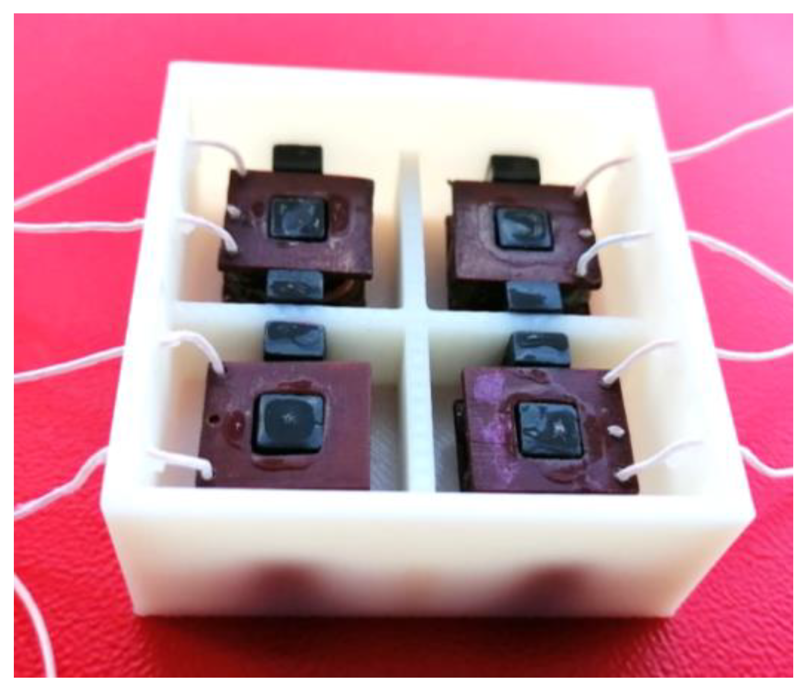
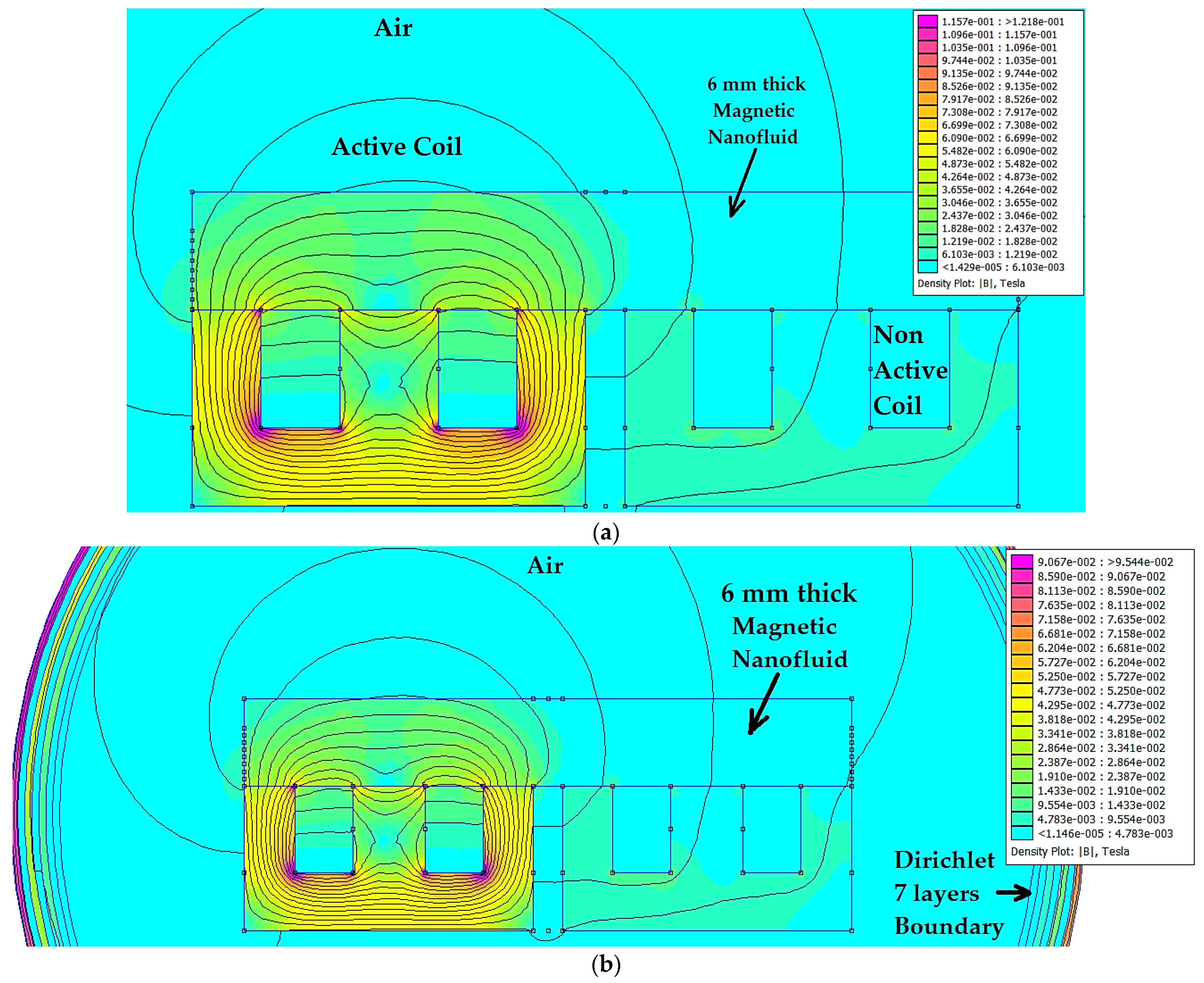
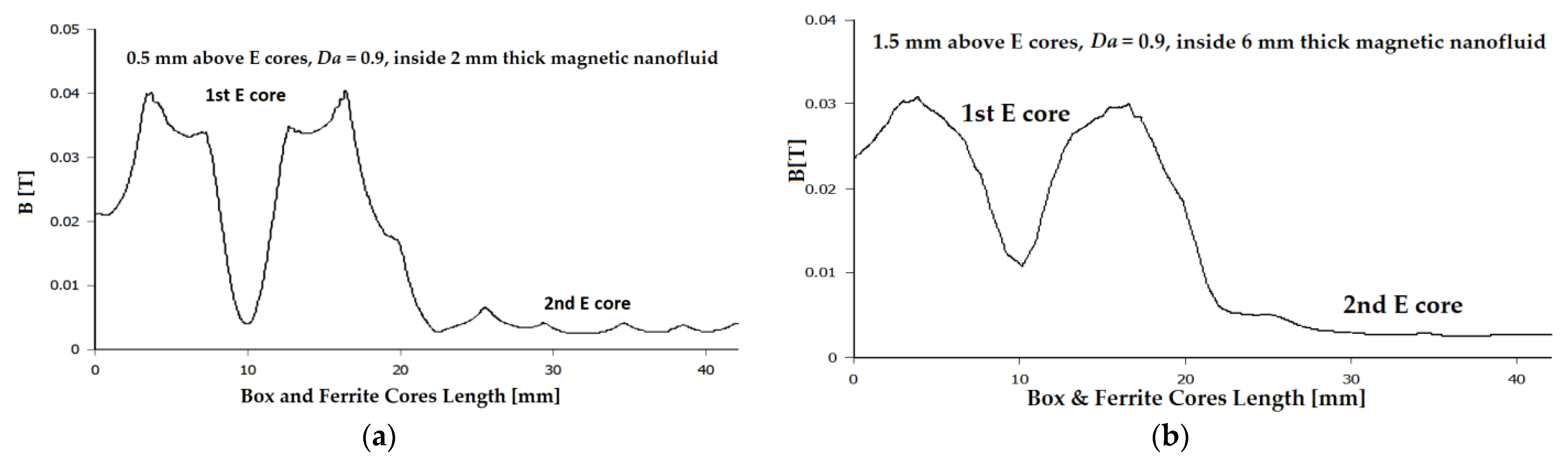
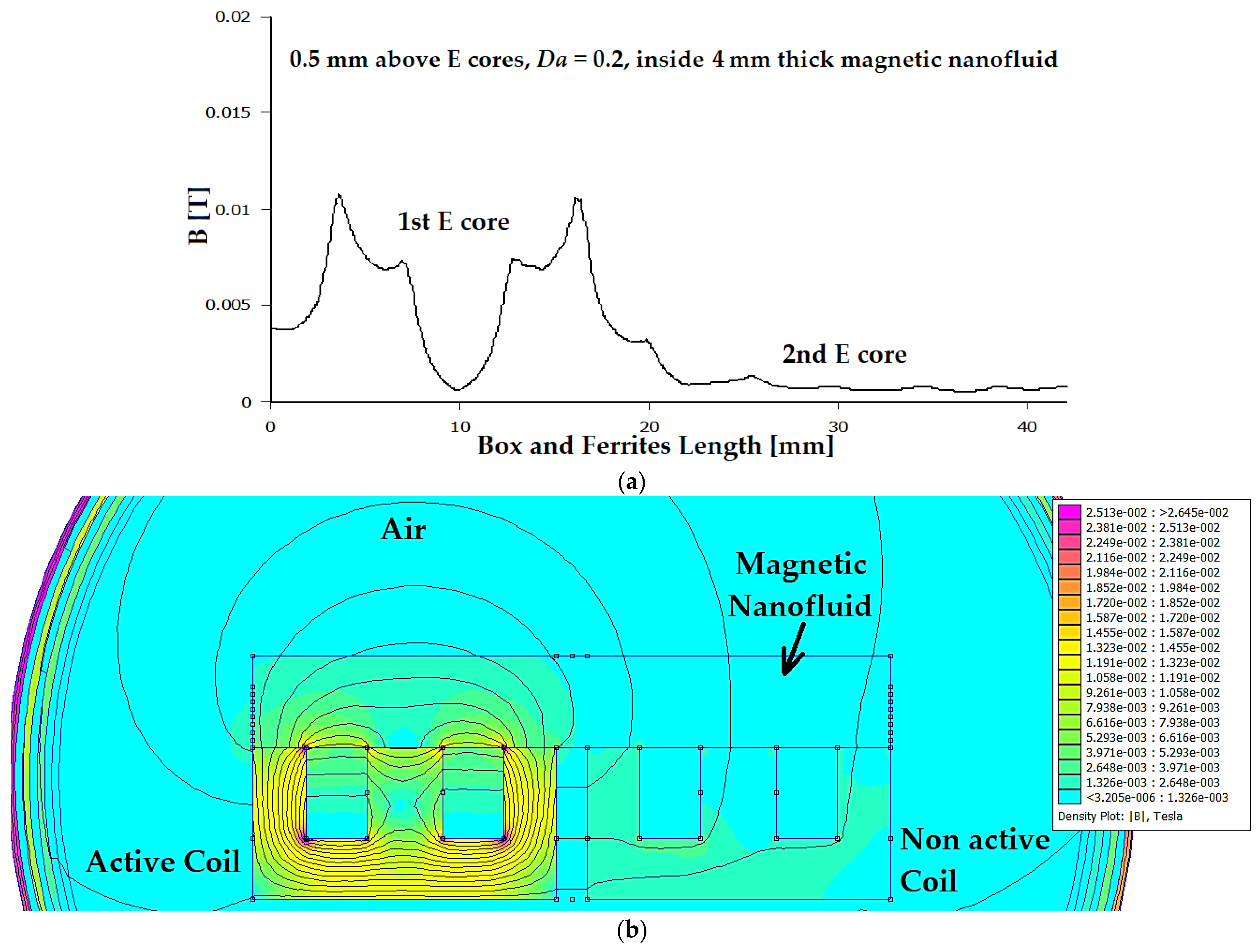
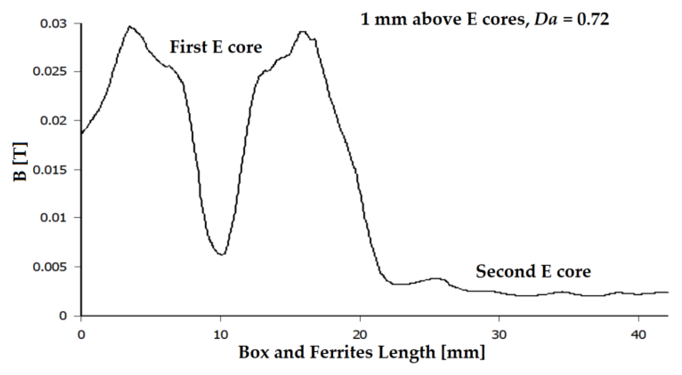
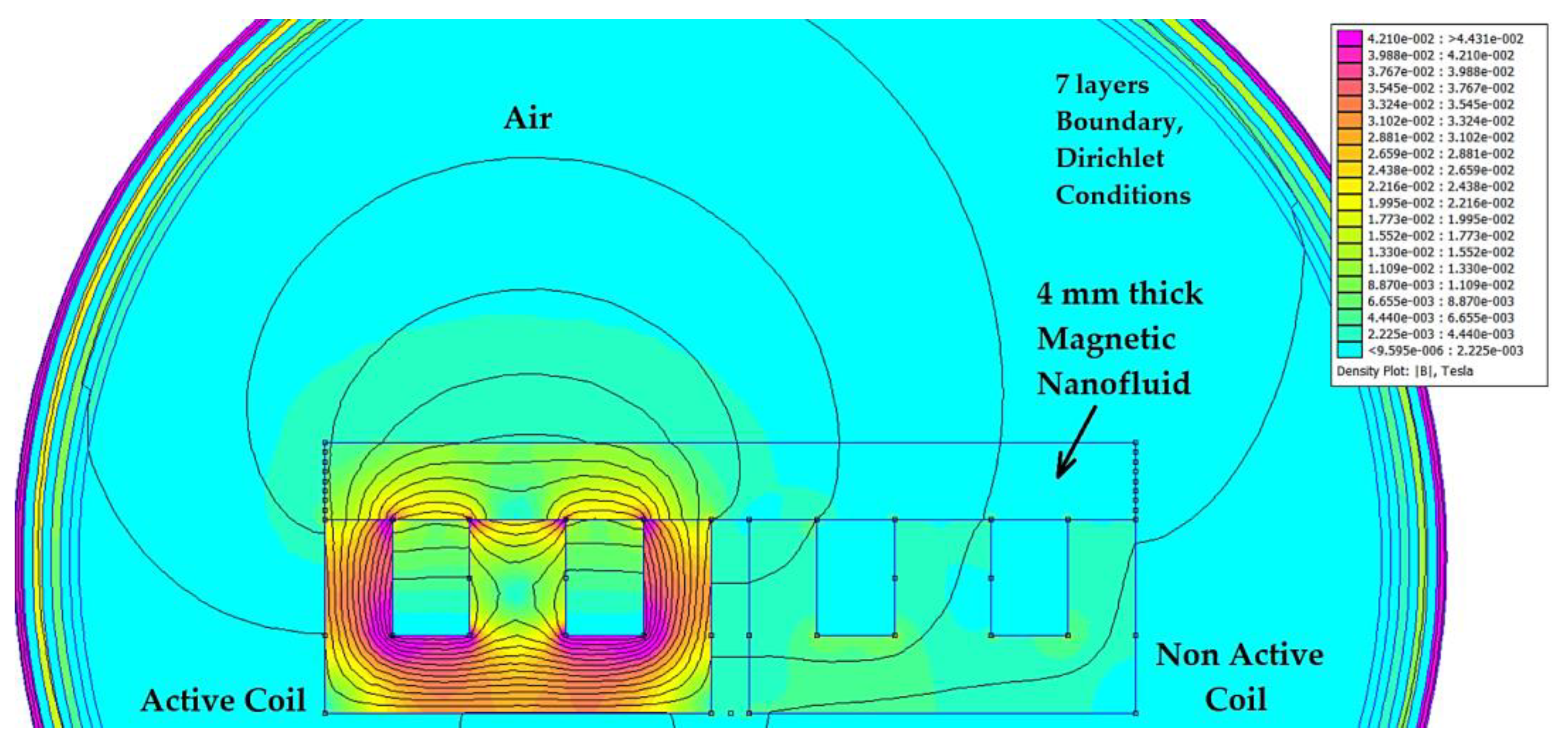
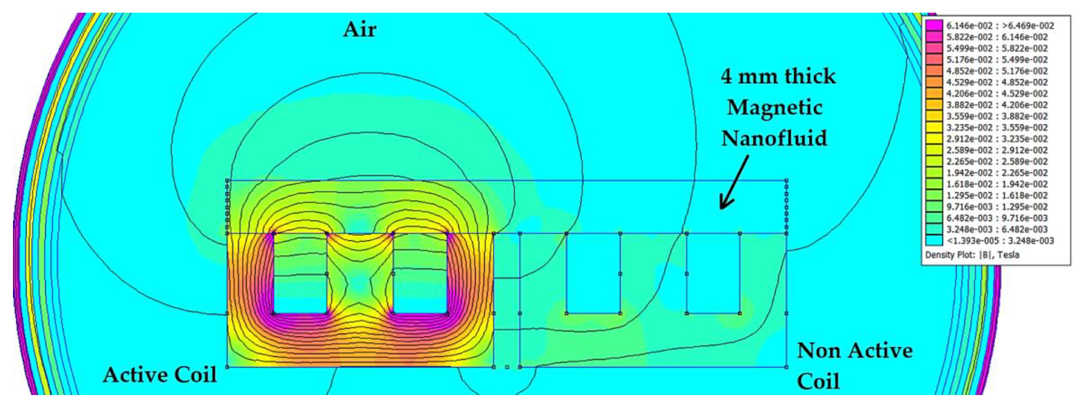
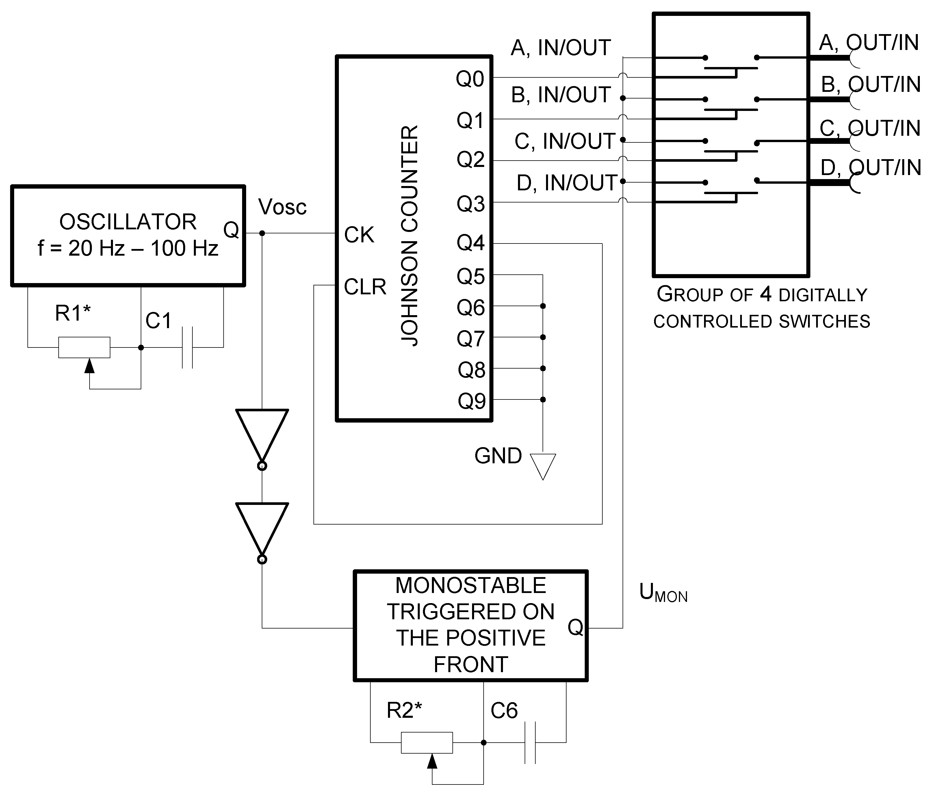
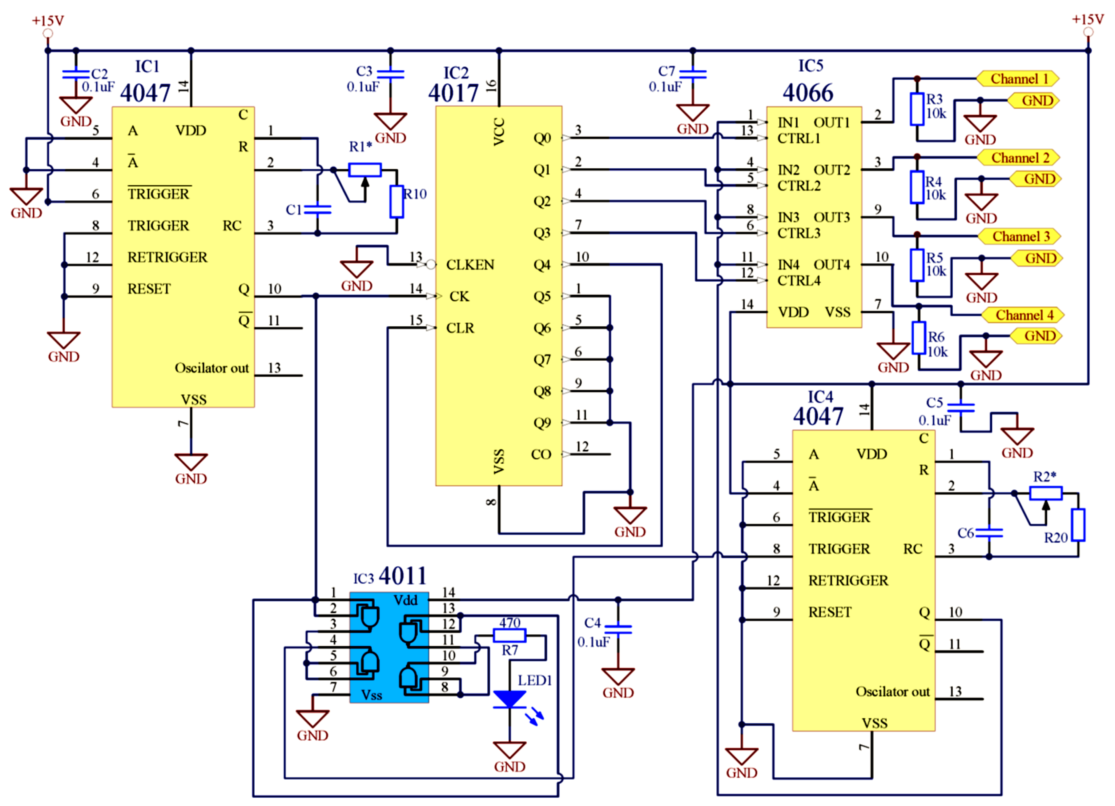
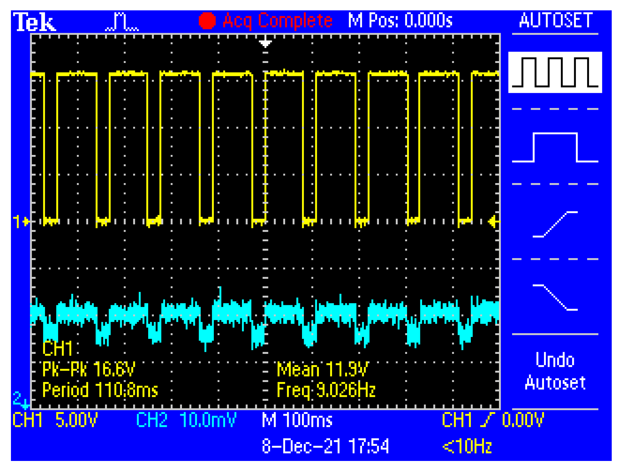
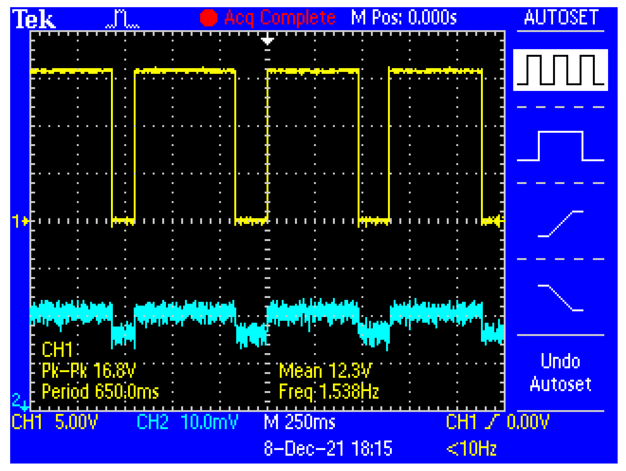
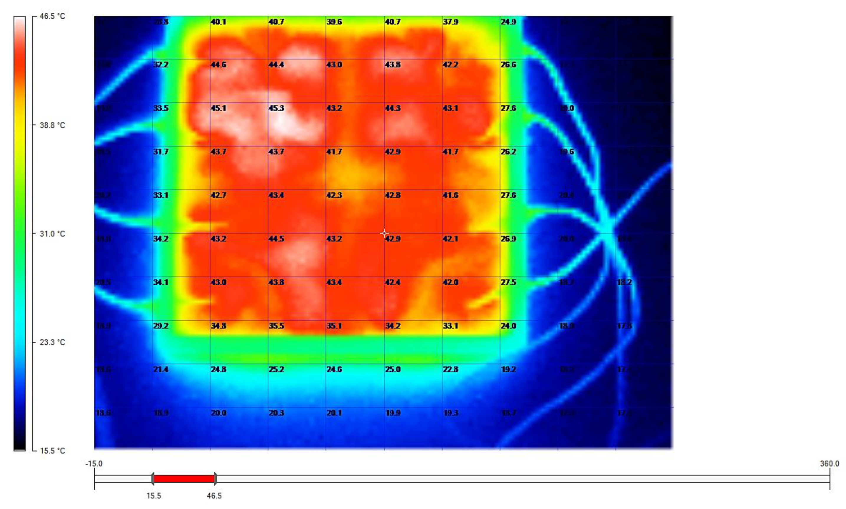
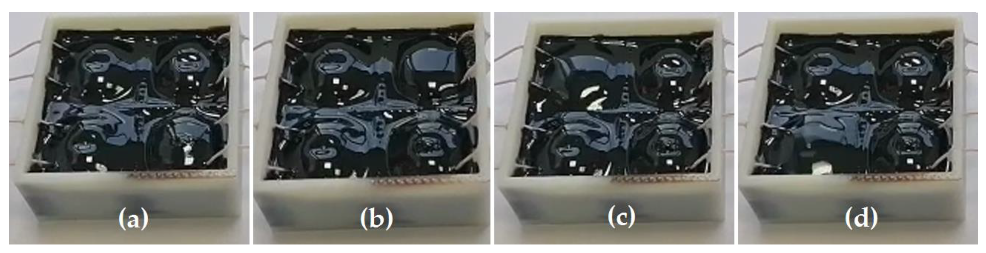
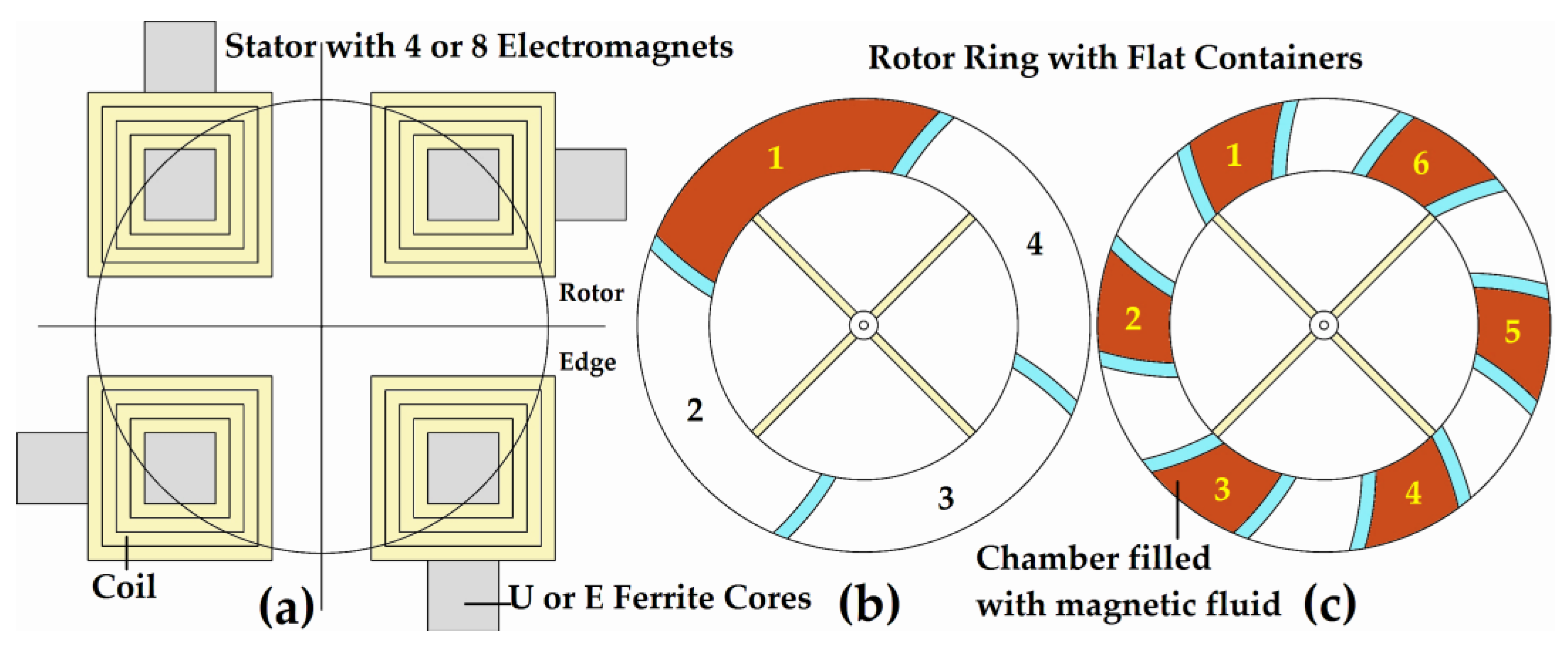
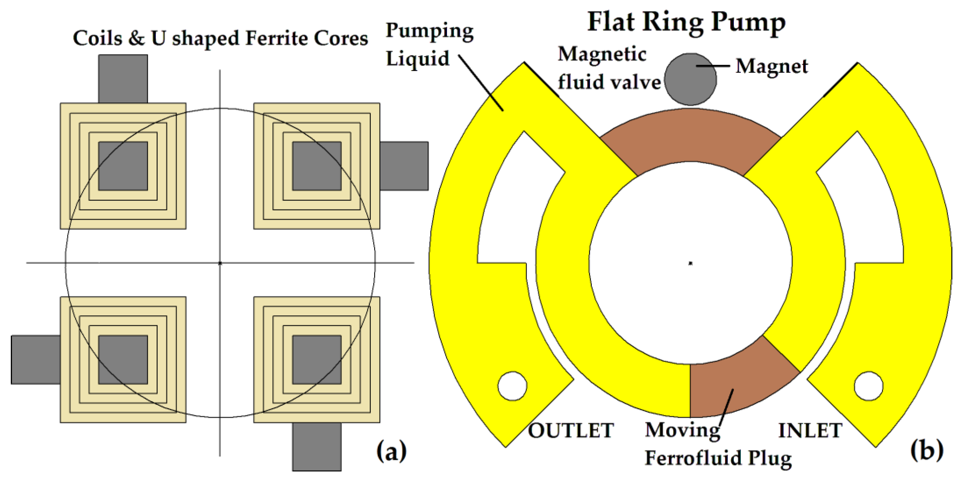
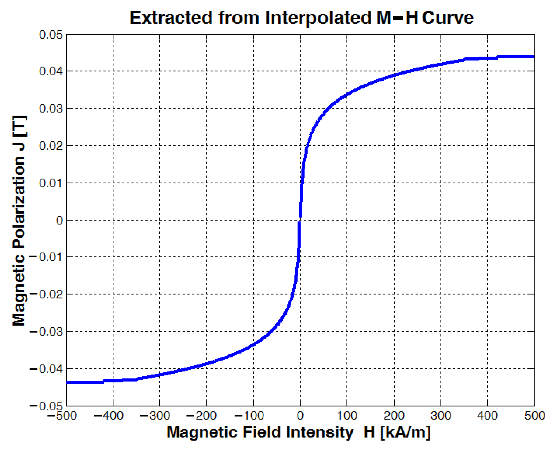
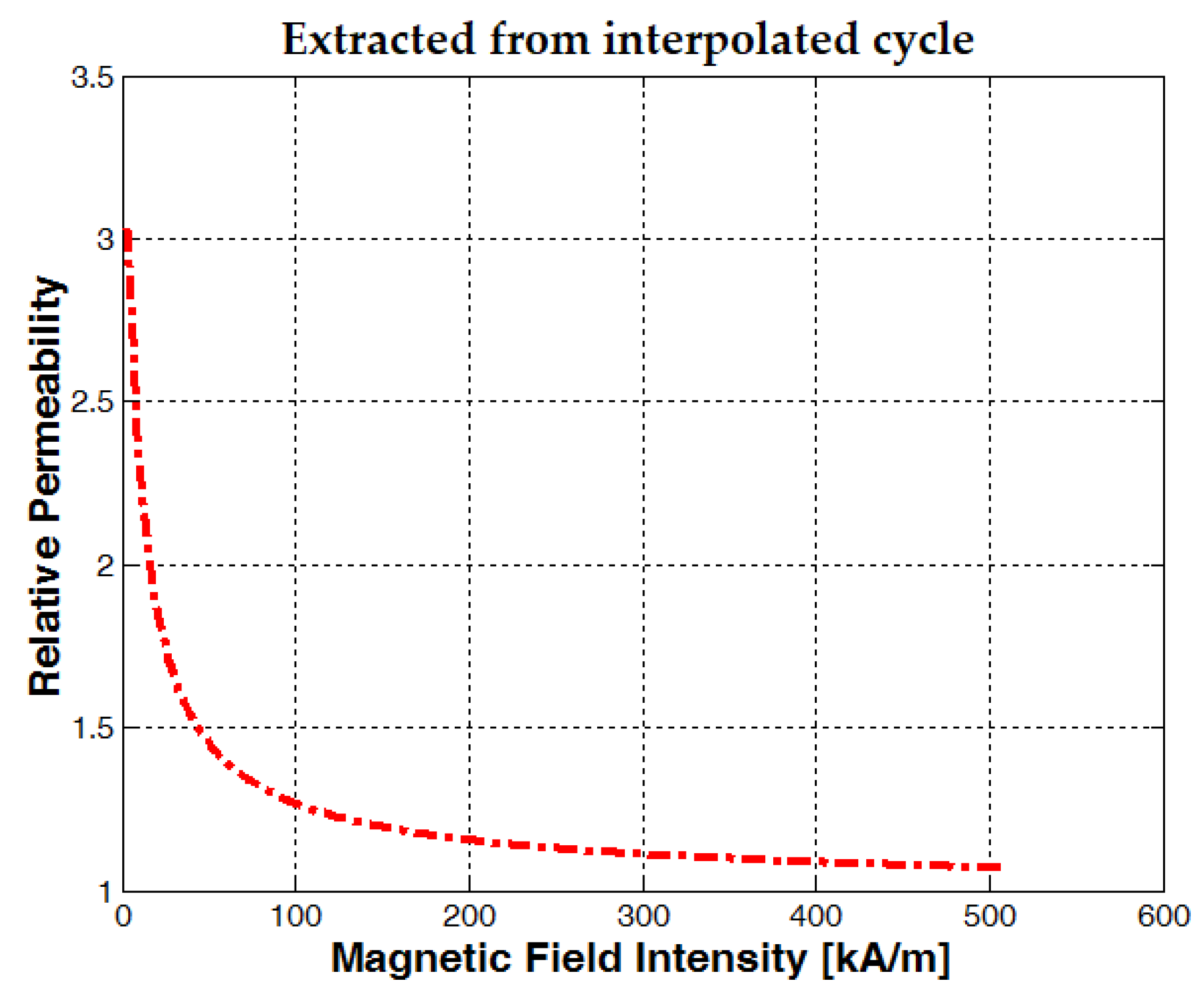
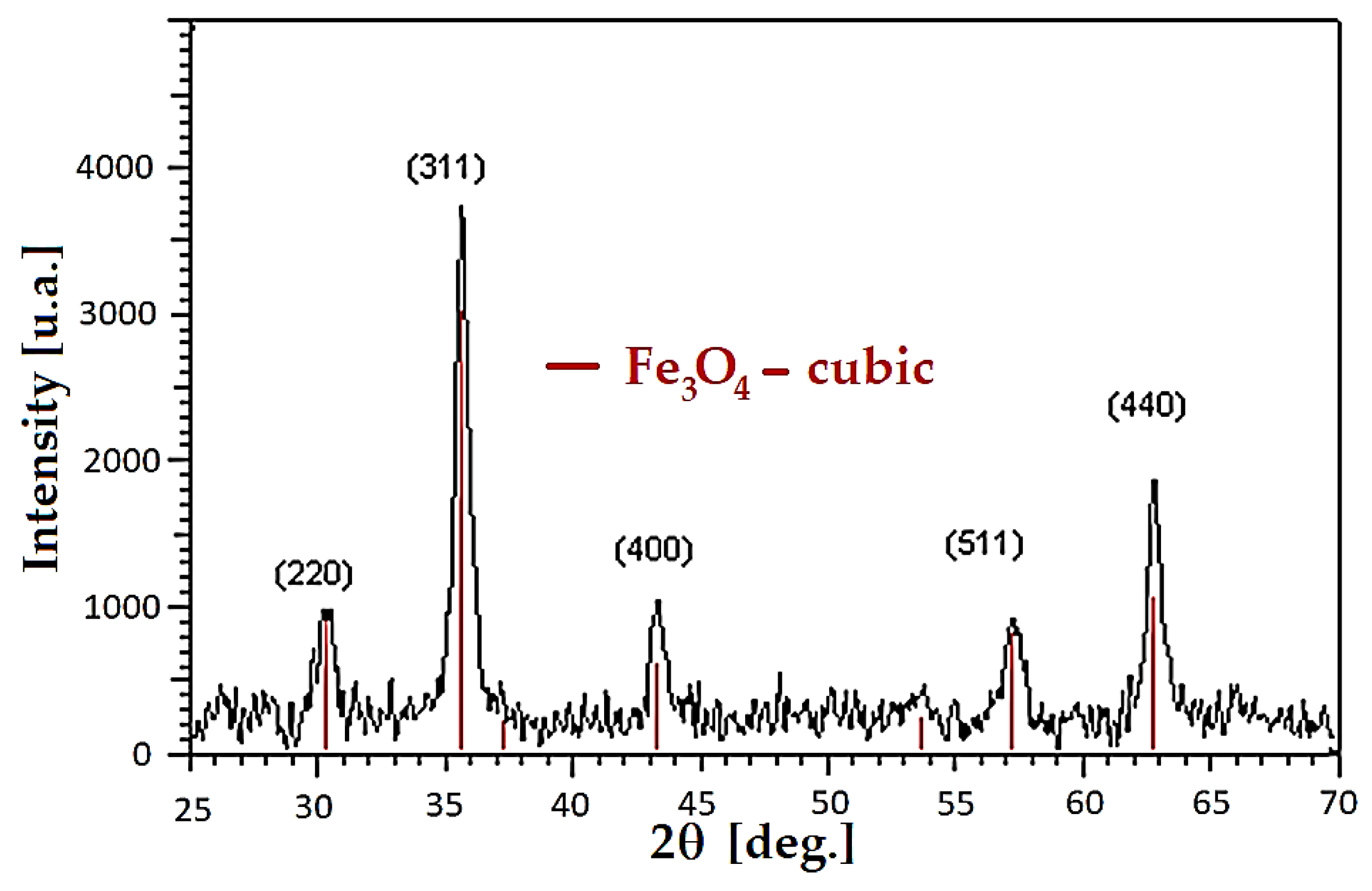
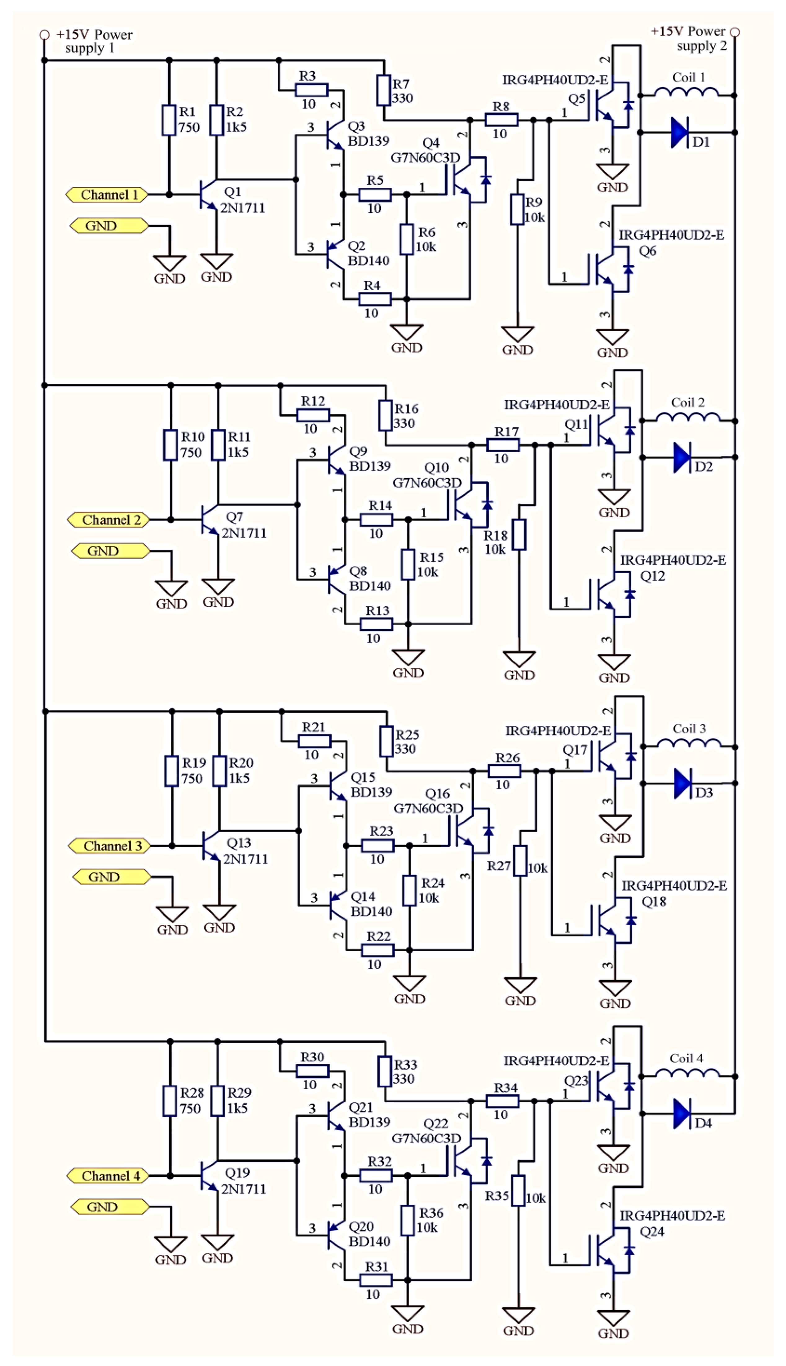
Table 1.
The magnetic field modeled for different Duty Cycle values and distances situated above two E cores, four different average currents were considered, 9.7 mA, 24 mA, 35 mA and 44 mA, each corresponding to 0.2, 0.5, 0.72 and 0.9 Duty Cycle and for 6 mm thick magnetic nanofluid.
Table 1.
The magnetic field modeled for different Duty Cycle values and distances situated above two E cores, four different average currents were considered, 9.7 mA, 24 mA, 35 mA and 44 mA, each corresponding to 0.2, 0.5, 0.72 and 0.9 Duty Cycle and for 6 mm thick magnetic nanofluid.
| Magnetic Field B[T] and Duty Cycle | 0.01 [mm] above | 0.5 [mm] | 1 [mm] | 1.5 [mm] | 2 [mm] | 2.5 [mm] | 3 [mm] | 3.5 [mm] | 4 [mm] | 6 [mm] |
|---|---|---|---|---|---|---|---|---|---|---|
| B[T] for Da = 0.20 | 0.010 | 0.0110 | 0.0070 | 0.0052 | 0.0044 | 0.0038 | 0.0031 | 0.0028 | 0.0025 | 0.0013 |
| B[T] for Da = 0.50 | 0.029 | 0.0280 | 0.0220 | 0.0190 | 0.0170 | 0.0150 | 0.0130 | 0.0110 | 0.0095 | 0.0033 |
| B[T] for Da = 0.72 | 0.044 | 0.0400 | 0.0300 | 0.0260 | 0.0240 | 0.0220 | 0.0190 | 0.0170 | 0.0160 | 0.0048 |
| B[T] for Da = 0.90 | 0.045 | 0.0440 | 0.0350 | 0.0300 | 0.0280 | 0.0250 | 0.0240 | 0.0230 | 0.0200 | 0.0060 |
Table 2.
Coil inductance, resistance and quality factor measurements at different frequencies.
| Series Configuration Measurements Ls, Rs. U = 2 V | |||||
|---|---|---|---|---|---|
| f [Hz] | Ls [mH] | Rs [Ω] | Z [Ω] | ϴr [mrad] | Q |
| 20 | 126.85 | 308.85 | 309.2 | 51.64 | 0.05 |
| 30 | 127.05 | 308.46 | 309.35 | 77.52 | 0.08 |
| 50 | 127.01 | 308.26 | 310.95 | 128.68 | 0.13 |
| 100 | 126.92 | 308.28 | 318.38 | 253.18 | 0.26 |
Disclaimer/Publisher’s Note: The statements, opinions and data contained in all publications are solely those of the individual author(s) and contributor(s) and not of MDPI and/or the editor(s). MDPI and/or the editor(s) disclaim responsibility for any injury to people or property resulting from any ideas, methods, instructions or products referred to in the content. |
© 2023 by the authors. Licensee MDPI, Basel, Switzerland. This article is an open access article distributed under the terms and conditions of the Creative Commons Attribution (CC BY) license (https://creativecommons.org/licenses/by/4.0/).
Share and Cite
MDPI and ACS Style
Pîslaru-Dănescu, L.; Zărnescu, G.-C.; Pătroi, E.-A.; Chihaia, R.-A.; Telipan, G. Microactuation of Magnetic Nanofluid Enabled by a Pulsatory Rotating Magnetic Field. Actuators 2023, 12, 210. https://doi.org/10.3390/act12050210
AMA Style
Pîslaru-Dănescu L, Zărnescu G-C, Pătroi E-A, Chihaia R-A, Telipan G. Microactuation of Magnetic Nanofluid Enabled by a Pulsatory Rotating Magnetic Field. Actuators. 2023; 12(5):210. https://doi.org/10.3390/act12050210
Chicago/Turabian StylePîslaru-Dănescu, Lucian, George-Claudiu Zărnescu, Eros-Alexandru Pătroi, Rareș-Andrei Chihaia, and Gabriela Telipan. 2023. "Microactuation of Magnetic Nanofluid Enabled by a Pulsatory Rotating Magnetic Field" Actuators 12, no. 5: 210. https://doi.org/10.3390/act12050210
Note that from the first issue of 2016, this journal uses article numbers instead of page numbers. See further details here.