
Distributed Cooperative Cruise Control for High-Speed Trains with Energy-Saving Optimization

1
School of Electrical and Information Engineering, Changsha University of Science and Technology, Changsha 410114, China
2
College of Automotive and Mechanical Engineering, Changsha University of Science and Technology, Changsha 410114, China
3
School of Computer Science and Engineering, Central South University, Changsha 410083, China
*
Author to whom correspondence should be addressed.
Actuators 2023, 12(5), 207; https://doi.org/10.3390/act12050207
Submission received: 21 April 2023
/
Revised: 11 May 2023
/
Accepted: 16 May 2023
/
Published: 17 May 2023
(This article belongs to the Section Control Systems)
Abstract
:With the aim of improving the energy utilization during the cooperative operation of multiple trains, this paper proposes an optimal distributed cooperative cruise control strategy to ensure safe and efficient tracking. A performance index function with distributed characteristics is constructed by considering the state errors among trains and energy consumption. An LQR-based optimal design technique is applied to cooperative cruise control to optimize the cooperative control gain to find the optimal solution. Additionally, the scalar coupling gains are introduced to decouple the design of the optimal cooperative control gain from the communication topology of trains. Thus, the proposed strategy is robust for arbitrary directed communication topologies and can eventually be used to achieve the distributed tracking optimization of multiple trains. The asymptotic stability of the system is proved strictly by exploiting the Hurwitz and Lyapunov stability theorem. A numerical simulation example is given to verify the feasibility and effectiveness of the proposed strategy.
1. Introduction
As high-speed railway technology is continuously developing and the number of trains is rapidly increasing, high-speed trains have gradually become an important part of China’s railway transportation. Undoubtedly, the increasing number of trains enables individuals to complete more transportation tasks together, which greatly improves the transportation efficiency. However, the shortening of the distance among trains poses a great threat to the operation safety. When the operating density increases, guaranteeing the safety distance among trains become a technical problem [1,2]. Nowadays, a novel train-centered communication-based train control (CBTC) system via train-to-train radio communication is proposed as an evolution direction for future transportation [3]. The train communicates directly with its neighboring trains through a wireless network to achieve cooperative control for autonomous resource management and active interval protection [4]. Therefore, a feasible multiple trains cruise control scheme is developed that can effectively solve the operation interval problem.
The implementation of train-to-train radio communication technology in high-speed railways has attracted numerous investigators to conduct in-depth research on cooperative cruise control for multiple trains, and they have obtained fruitful achievements [5,6,7,8,9]. It is an interesting research topic in which each train dynamically adjusts its speed and position by communicating with neighboring trains. Ning et al. [5] proposed a cooperative model with a back-fence communication topology, which was used to design a distributed cooperative controller for high-speed trains under a moving block system. Li et al. [6] considered the presence of unknown parameters in the system and proposed an adaptive distributed cooperative control strategy to identify the unknown parameters. Lin et al. [7] addressed the problem of the cooperative tracking control of multiple trains with a distributed speed and input constraints and put forward the model transformation and convex analysis method, whereby all trains are guaranteed to run in a stable mode and track the required speed. Gao et al. [8] addressed the problem of cooperative control for multiple high-speed trains to achieve the required performance tracking; that is, to ensure that the speed and position of high-speed trains are respectively limited within the specific speed limit and allowable distance approved by the automatic train protection and moving authorities. Wang et al. [9] improved the potential function in [6] and proposed a new cooperative cruise control strategy, where interestingly, the safety distance between trains could be dynamically adjusted according to the train speed.
However, the previous cooperative cruise control that only focuses on improving the operation efficiency (running safety, speed tracking) is not realistic. The energy consumption of the cooperative operation of multiple high-speed trains poses an increasing threat to the ecological environment, which is not conducive to the long-term development of railway transportation in the current context of the increasing energy shortage [10,11]. Thus, energy-saving optimization is another indispensable performance index that needs to be considered in addition to the operation efficiency.
Some existing research reports have token energy-saving optimization as the key objective for the control problem of multiple high-speed trains. Huang et al. [12] proposed a comprehensive energy-saving operation optimization method for multiple trains between multiple stations by considering regenerative braking. Chen et al. [13] aimed to minimize the total energy consumption for multiple trains by optimizing and updating speed curves and considering the regenerative braking power losses on the catenary. In order to minimize the difference between traction energy consumption and regenerative energy consumption, Su et al. [14] proposed a comprehensive train operation method by jointly optimizing the train schedule and driving strategy. From the energy-saving perspective, these discussions can effectively improve the energy efficiency, but they are not distributed cooperative control methods. The state information of neighboring trains transmitted by the network are ignored and useless. The minimum safe distance is also not preserved.
Therefore, it is crucial to design a cooperative cruise controller that can simultaneously solve the operational safety, speed tracking and energy saving issues, which will be another urgent and attractive problem and of important practical significance. Motivated by the above analysis, this paper will design a distributed cooperative cruise controller for multiple trains with energy-saving optimization. Moreover, LQR optimization is widely used in the energy optimization of a single train operation [15,16], which could minimize the performance index function by designing a control gain. Since the optimal control gain of linear feedback can be obtained, it is easy to construct a closed-loop optimal control to obtain the minimum possible energy consumption [17,18,19,20].
In this paper, in order to combine the advantages of both LQR and the distributed cooperative control, a cooperative control strategy based on a leader-following multiagent system distributed-consensus algorithm is proposed, and a performance index is constructed by considering the relative state errors and energy consumption. An LQR-based optimal design technique is introduced when designing the cooperative cruise control to optimize the cooperative control gain in order to find the optimal solution and achieve the minimum tracking error and energy consumption when it comes to the cooperative operation of multiple trains. Additionally, it is worth noting that a scalar coupling gain is also introduced to decouple the design of the optimal cooperative control gain from the train communication topology, which weakens the impact of the communication topology. Numerical examples illustrate the rationality of the proposed distributed optimization approach. Compared with the existing studies, the major contributions of this report are described as follows:
- An optimal distributed cooperative cruise control strategy for multiple trains is proposed, in which the LQR optimal design technology is exploited to optimize the cooperative control gains, such that the speed of all trains can rapidly converge to the desired speed curve with an efficiently reduced energy consumption.
- The proposed control strategy is robust for arbitrary directed communication topologies. A scalar coupling gain is introduced to decouple the design of the cooperative control gain by using information on the topological structure characteristics as they pertain to the system stability, and the optimality of the cooperative control can be ensured by properly selecting the scalar coupling gain.
- It is strictly proved that the multiple train system can eventually achieve asymptotic stability with the proposed optimal distributed cooperative control.
The rest of this report is structured as follows. The longitudinal dynamics model and the related communication topology principle of multiple high-speed trains are presented in Section 2. In Section 3, an optimal distributed cooperative control strategy based on LQR is designed for each high-speed train, and the stability of the system is proved. In Section 4, two control strategies are simulated and compared to verify the feasibility of the proposed method. In Section 5, we give a brief summary.
2. Problem Formulation
The present section mainly carries out two works. In the first work, a longitudinal nonlinear dynamic model that can capture the main characteristics of train dynamics is constructed. In the second work, we use graph theory to describe the communication relationships between adjacent trains.
2.1. Dynamic Model of High-Speed Trains
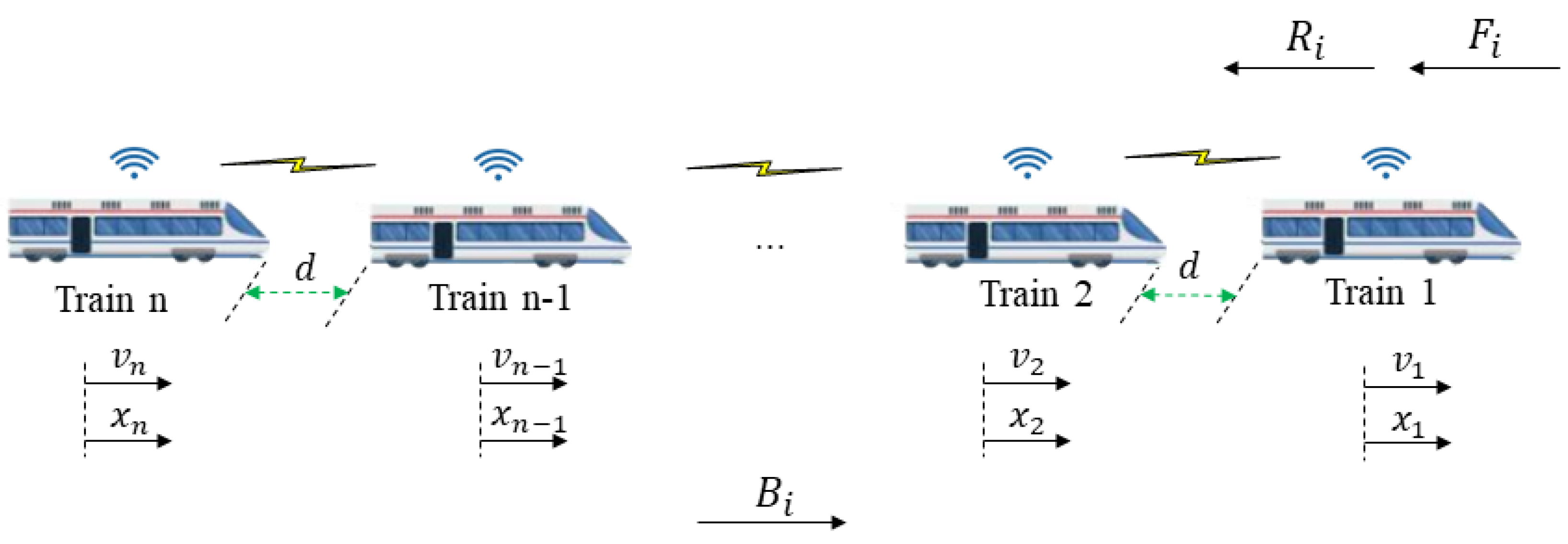
The cruise control system of multiple trains that is investigated in this paper consists of n trains with double integrator dynamics, and each train is strictly defined as a rigid particle, which is plotted in Figure 1. In actual operation, the safe distance is far greater than the length of the train, so it is quite regular to regard the train as a rigid particle from the viewpoint of practical considerations [21]. In Figure 1, it can be observed that the longitudinal force of high-speed trains mainly includes three types of forces, namely, the traction force in the direction of motion, the braking force and the resistance force in the opposite direction of motion. The resistance force is generally composed of basic resistance and additional resistance. The basic resistance exists throughout the entire operation of the train, while the additional resistance only exists on special routes such as slopes, curves and tunnels.
The basic resistance is mainly composed of two parts, namely, mechanical resistance and aerodynamic resistance. The mechanical resistance is composed of rolling friction, which is generated by the train wheels running on the railway track; sliding friction, which is caused by the wheels sliding on the railway track; impact and vibration resistance, which is caused by the wheel–rail impact and vibration during rolling; and bearing friction resistance, which is generated by the relative movement between the bearing and its inner and outer rings during rolling. The aerodynamic resistance is the running resistance generated by the relative movement between the train body and the air during the operation, which includes pressure difference resistance and air friction resistance. When conducting experimental calculations on these resistances, due to the influence of various factors such as the train type and operating conditions, standard measurement values cannot often be obtained. Therefore, it is frequently represented by the Davis equation [22] when designing the train control system based on the train dynamics model. The additional gravitational resistance and curvature resistance are considered. The total resistance is expressed as follows:
where denotes the mass of the train i. , , denotes the resistance coefficients, which can be obtained through wind tunnel experiments [23], and its value is impacted by many factors, such as the train type, operating conditions, etc. The first two terms denote the rolling mechanical resistance and the third term is the air resistance. The gravitational and curvature resistance forces experienced by the train are and , respectively.
Based on the above force analysis for high-speed trains, by Newton’s second law of motion, the nonlinear dynamics model of the trains can be described by the following differential equation:
in which , denotes the actual position and speed. It is important to note that refers to the braking force or tractive force of each train. The target of this work is to obtain an optimal distributed cooperative control strategy , such that the positions and speeds of each train could be governed by controlling their accelerations, to reduce the unnecessary energy consumption caused by the train during traction or braking and to guarantee an adequate level of efficiency and energy-saving with the train operation.
2.2. Communication Network Topology among Trains
Graph theory is typically used to explain the communication relationships between agents in multiagent systems. In this section, some facts about graph theory used in this paper are reviewed. For the running convoy containing n trains, each train is considered as an agent, and the state information is transmitted through the communication between the trains to reach a consensus. Let be a directed graph, in which , is a set of trains that mean the number of trains and is constituted by a set of edges. If , then it means that these trains can communicate with each other and there is an edge between them. refers to the adjacency matrix of the graph, denoted by , which is usually used to describe the communication connectivity between trains. If the ith train can communicate with the jth train, then , otherwise . The in-degree matrix represents the number of the trains that train i can receive information from, and the Laplacian matrix is described as . For a directed graph, L always has an eigenvalue 0 if it contains a directed spanning tree.
3. The Cooperative Controller Design
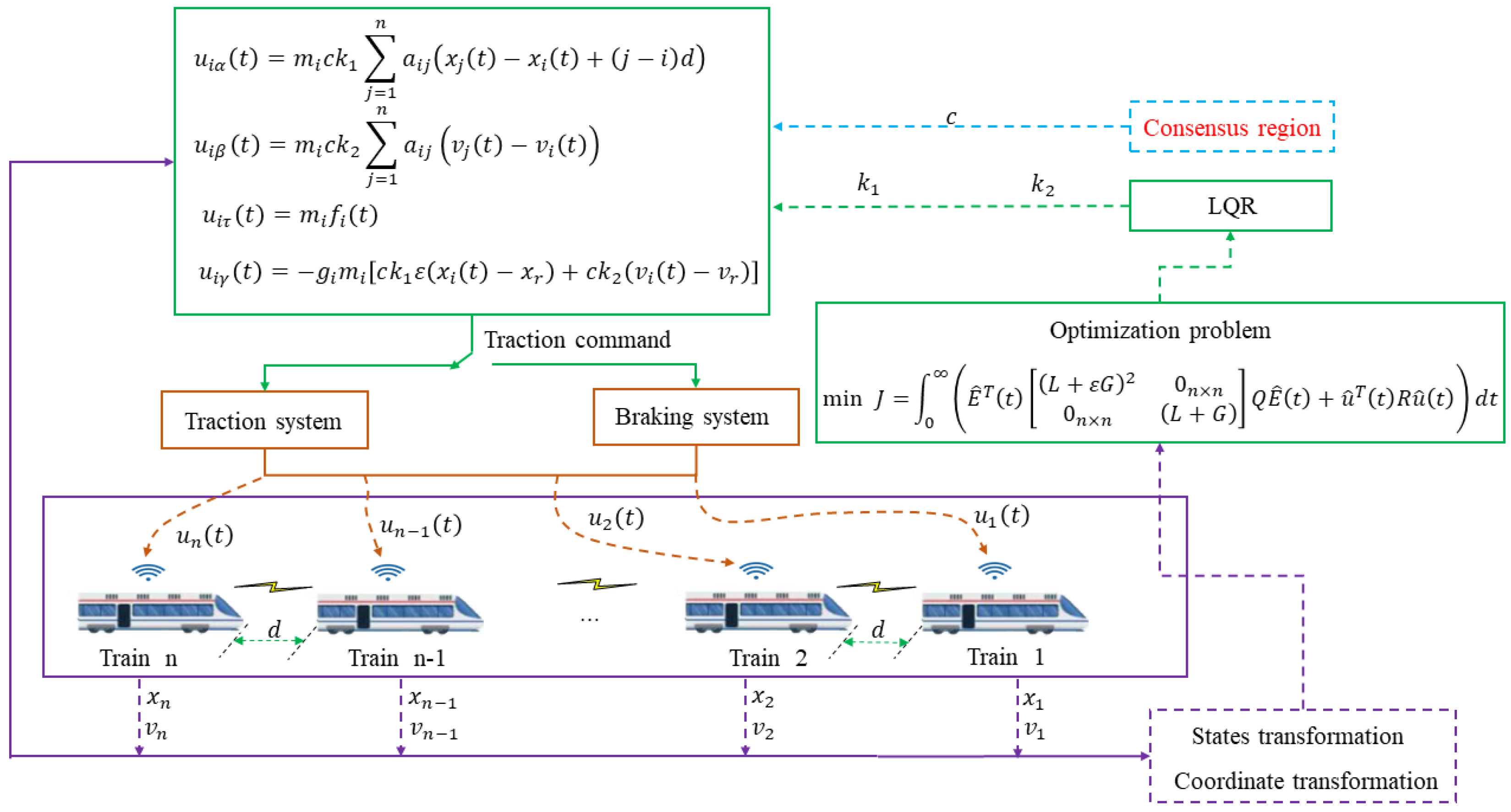
This section describes the design of an optimal distributed cooperative control strategy for multiple trains, which combines distributed consensus algorithms and optimization algorithms. Figure 2 depicts the fundamental framework of the proposed control strategy. The controller for each train is composed of four parts, and the specific details are elaborated in the following section. On this basis, a performance index function with distributed characteristics was established, which includes three types of performance indexes: the relative speed error, relative distance error and energy consumption. Subsequently, the optimization algorithm was utilized to solve and obtain the optimal cooperative control gains and to achieve the objective of energy-saving optimization. Finally, the concept of a consensus region is introduced, and the necessary and sufficient conditions of scalar coupling gain c are derived.
3.1. The Basic Cooperative Control Strategy Design
Compared with the traditional CBTC system, the CBTC system framework based on train-to-train communication is simplified, the number of trackside equipment is reduced, and the most important action is to decrease the communication delay. Therefore, we temporarily presumed that there was a communication delay in the tolerable range when analyzing the system [24]. Then, we proposed a distributed cooperative control strategy and gave the following definitions:
Definition 1.
The control strategy designed for the system model in (1) has the following two features:
- 1.
- The rear trains receive information about the states of the preceding train at all times and adjust their states in time until all trains are tracking the desired speed
- 2.
- The interval among the trains can be kept at a safe distance under all the transient responses, and the trains can eventually converge to a fixed distance.
The proposed distributed cooperative control strategy for each train is determined to contain the following four components:
where refers to a formation control term, which is used to promote the alignment of the displacement state information. In , d is the desired distance among trains, which is always given as the minimum safe distance of each line. represents the interaction of speed state information between the trains. is used to overcome the effects of basic resistance and gravitational and curvature resistance force. indicates that each train can quickly follow the curve trajectory of the virtual leader train after a period of time, and all trains have a unified desired speed and desired position , where is a positive constant to overcome the defect of a large speed error at the initial time caused by the position error. is the pinning gain matrix element, which provides a definition as follows:
Definition 2.
is used to identify whether the train i can receive the information from the virtual leader train without a loss of generality; if so, then , otherwise .
From the above, the distributed cooperative optimized control strategy for each train in this paper has the following form:
in which c is the scalar coupling gain. and are the cooperative control gains to be determined by the designer, which are related to the control performance. In particular, the function of the first item in Equation (4) is to achieve a distributed consensus among the trains, and its requirement is that the communication topology needs to contain a directed spanning tree.
3.2. States Transformation and Coordinate Transformation
When each high-speed train is tracking the desired speed, its real-time speed is and its real-time position is , in which denotes the initial time and represent the end time. In order to obtain the error dynamics model of the multiple trains system, we defined , as the position error and speed error, respectively. Combining (1) and (4), the error dynamics model of the high-speed train can then be derived:
It is obviously observed from model (5) that the existence of the safety distance d is not conducive to the subsequent transformation of the model into a standard linear system model. Therefore, the formation tracking problem is transformed into a basic consensus problem by introducing coordinate transformation (6) [25]. Let
Under (6), we can obtain that
Based on (6) and (7), the error dynamics model (5) could be rewritten as
where
The error dynamics Equation (8) could be formulated as a fundamental linear compact state-space model:
where the state matrix , the input matrix , and ; denotes the error states of the multiple trains system and indicates the error of the control input.
3.3. The Optimal Cooperative Control Design
Although the cooperative control gains given freely based on the control performance can optimize the control performance, the analysis process does not give a clear performance index to measure the operation performance and energy consumption, and it is difficult to consider the optimization problem by integrating the energy consumption and operation performance [5,6,7,8,9]. To meet the requirements of safe tracking and energy saving during the cooperative operation of high-speed trains, it is an effective method to design a cooperative control strategy by adopting optimal control ideas under the constraints of a performance index function.
Based on state errors among neighboring trains and energy consumption, the following performance index function is constructed for each train [26]:
where , and are adjustable weighting parameters. The first two terms represent the relative state error between the trains, which improves the operation efficiency by minimizing the error. The third term referring the control input represents the energy consumption for the operation, which is minimized to achieve an energy-saving optimization.
Since this paper focuses on the multiple trains cooperative operation optimization problem, and considering that the global optimal solution can be easily obtained by using the global performance index, the performance index function including all trains is obtained on the basis of (10), and its global form is given as follows:
where , , and .
When finding an optimal control input error , the performance index function can be minimized, which means that the performance index reaches the optimal level when the system is stable:
where is the optimal cooperative control gain matrix to be designed. is the scalar coupling gain matrix. is the global error states with elements and .
Then, the global error dynamics of the closed-loop system is given as
where .
3.4. Stability of the System
The criterion for the asymptotic stability of the system and the necessary and sufficient condition to obtain a scalar coupling gain to satisfy the unbounded consensus region are given below.
Lemma 1
([19]). Let and denote the eigenvalues of L and G, where , and are the real and imaginary parts of the eigenvalues, respectively. Only when the matrixes
are Hurwitz, the closed-loop system (12) can guarantee asymptotic stability.
From Lemma 1, it can be determined that the arbitrary cooperative control gains and may not achieve consensus under the specified communication topology. In Theorem 1, the method of obtaining the optimal cooperative control gains is given to ensure the stability of any directed graph including the spanning tree by using the optimal design based on LQR and selecting the coupling gain c correctly. Before that, we introduce the concept of the consensus region as shown below.
Lemma 2
([19]). The consensus region reflects the robustness of the consensus. The larger the scope of a system’s consensus region, the easier it is to converge. An unbounded consensus region is more convenient for the design of a cooperative control strategy than a bounded consensus region, so it is necessary to find an unbounded consensus region for a cooperative control strategy based on the consensus algorithm. Define the consensus region S: if
the demonstrates asymptotic stability.
Theorem 1.
Assuming that both and are symmetric positive definite matrices, that is, and , then the cooperative control gain K is obtained as follows:
in which P is the solution of the Riccati equation, which is the symmetric matrix, namely
where ,
For the distributed cooperative control strategy (4), if the optimal cooperative control gain is selected according to Equation (16), then the consensus region is unbounded and there is a conservative consensus region that satisfies
The global error dynamics (14) are asymptotically stable if the scalar coupling gain c satisfies the following conditions:
Proof.
Using Equations (16) and (17), perform the following mathematical transformations by substituting Equation (14) into the Lyapunov equation:
Since the matrix is a complex matrix, it is known from matrix theory that each element needs to be conjugated before transposing it; thus, we can obtain that:
□
Since , , if holds, that is, Equation (19) satisfies the condition, can achieve gradual stability. Similarly, replace with s in the above transformations, and Equation (18) meets the requirements, which means that the proof is completed.
Remark 1.
In this paper, we only consider the cooperative cruise operation for multiple trains on a high-speed railway mainline. In other words, our work excludes the communication topology changes caused by the following operational conditions: (1) There are other trains merging into the railway mainline. (2) There are trains exiting from the railway mainline. Therefore, the communication topology between trains given in this paper is always a fixed directed graph with a spanning tree. Thus, the matrices and always have positive real parts for the eigenvalues.
Remark 2.
Consider the impact of some irregular events that may exist in reality (e.g., extreme weather, complex terrain, etc.) on the communication topology. The introduction of scalar coupling gain c can decouple the design of optimal cooperative control gain K from the communication topology of trains, which means that the change in the communication topology will not have any negative effect on multiple trains’ cooperative control. Therefore, the proposed distributed cooperative strategy is robust for any communication topology.
Remark 3.
It is worth noting that the lower bound of the scalar coupling gain (19) is related to the second smallest eigenvalue of the Laplacian matrix and the largest eigenvalue of the pinning matrix, because both of them are directly linked to the states’ convergence speed. By properly selecting the scalar coupling gain, and can be used to solve the multiple trains’ tracking control problem, and it is meanwhile not necessary to recalculate for different and , which thus reduces the computational complexity.
Remark 4.
The weight matrix contains the eigenvalues and of global information and , which are related to the maximal eigenvalues and , which means the distributed optimization cannot be achieved. To avoid using the global information and , we can use their upper bound and in (16), which can be obtained in terms of the maximal node degree by using the Gershgorin Disk Theorem, i.e.,
4. Simulation Results
In this section, the effectiveness of the proposed control strategy is evaluated through numerical simulations. First, the necessary preliminary work for the simulation is introduced, including some basic parameters of the trains that are required. Secondly, for the trains with an initial speed of zero, the basic distributed cooperative control strategy, the control strategy proposed in the literature [7] and the optimal distributed cooperative control strategy in this paper are simulated, and the control performance and energy consumption of the trains under these three control strategies are compared. Finally, the optimal distributed cooperative control strategy is simulated and analyzed for the trains with a nonzero initial speed, and the consensus capability of this control strategy is verified.
4.1. The Simulation Parameters Setup
There were five trains with an equal weight running sequentially on a straight high-speed railway with weights of t. The resistance coefficient N/kg, Ns/mkg and Ns2/m2kg were obtained from [27]. For the desired safe distance among adjacent trains, we chose a fixed distance of km. The simulation time was s, and the positive constant . The pinning gain matrix . The adjacency matrix corresponding to the directed communication topology between trains was as follows:
In terms to the method of Remark 4, we used twice the maximal node degree to evaluate the upper bound of the maximal eigenvalue as and . We chose , and .
4.2. Zero Initial Speed
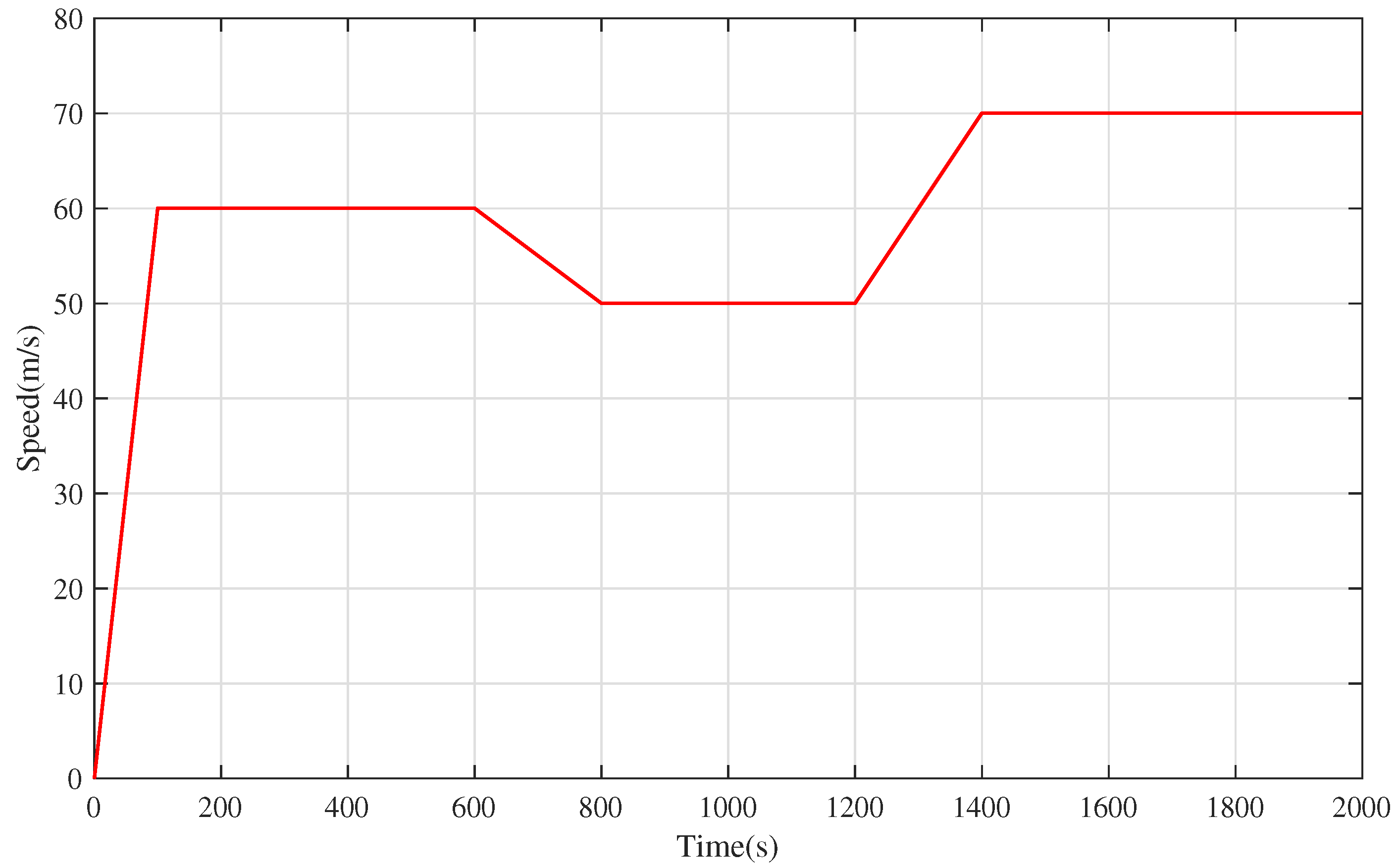
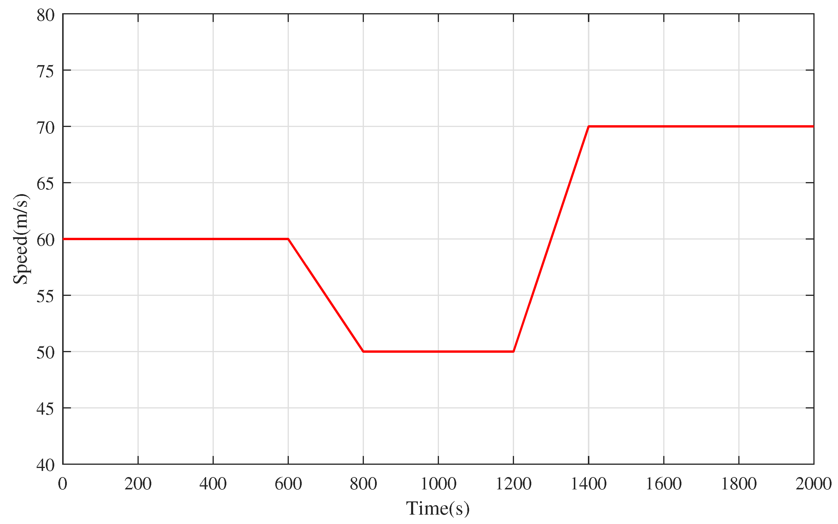
In this section, the initial positions and speeds are given in Table 1, and the speed trajectory of the virtual leader train operating in the following time periods, which are composed of two acceleration phases, three cruising phases and one deceleration phase, is also given. The prescribed trajectory is given in Figure 3.
4.2.1. Simulation Test for the Basic Cooperative Control Strategy
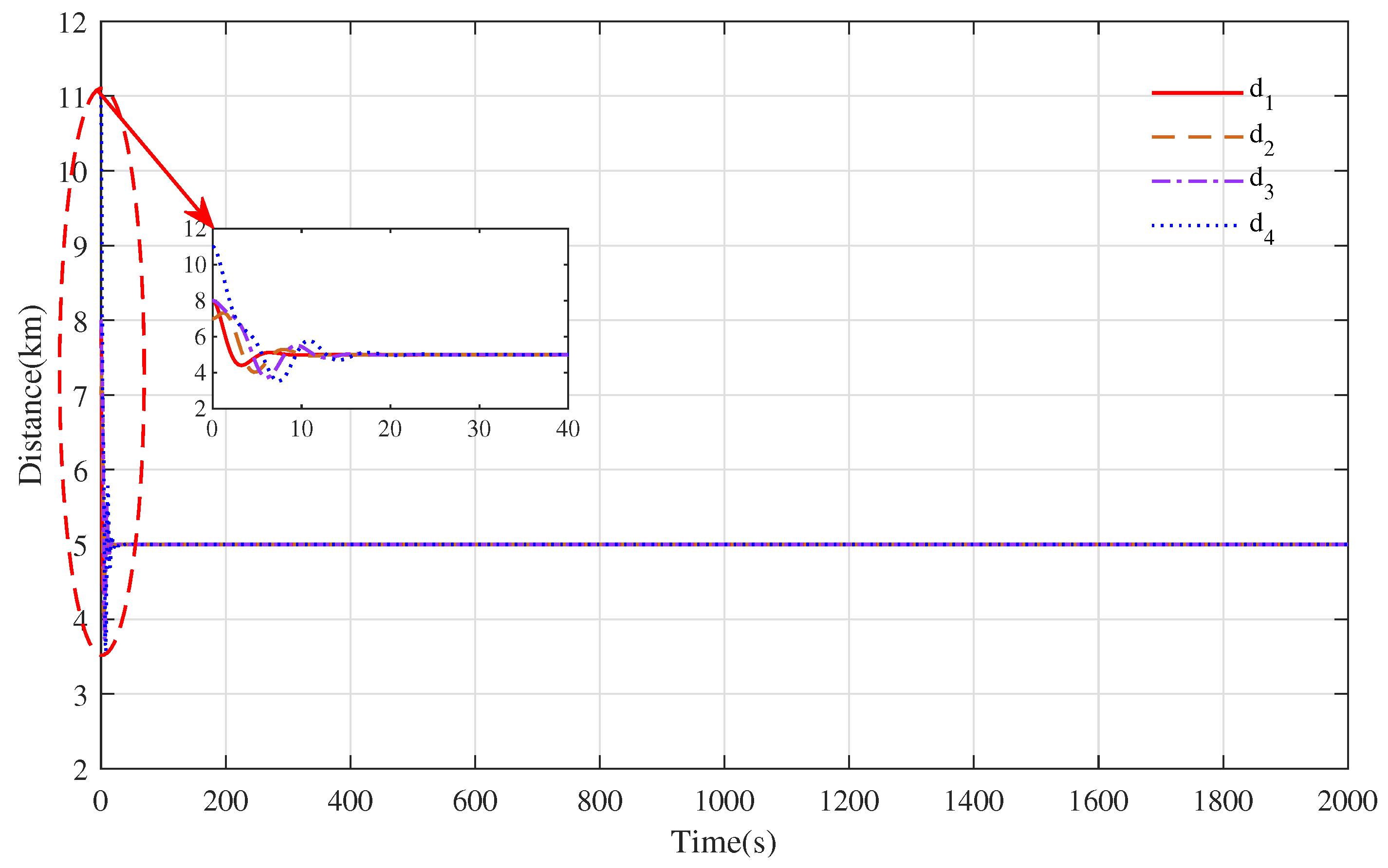
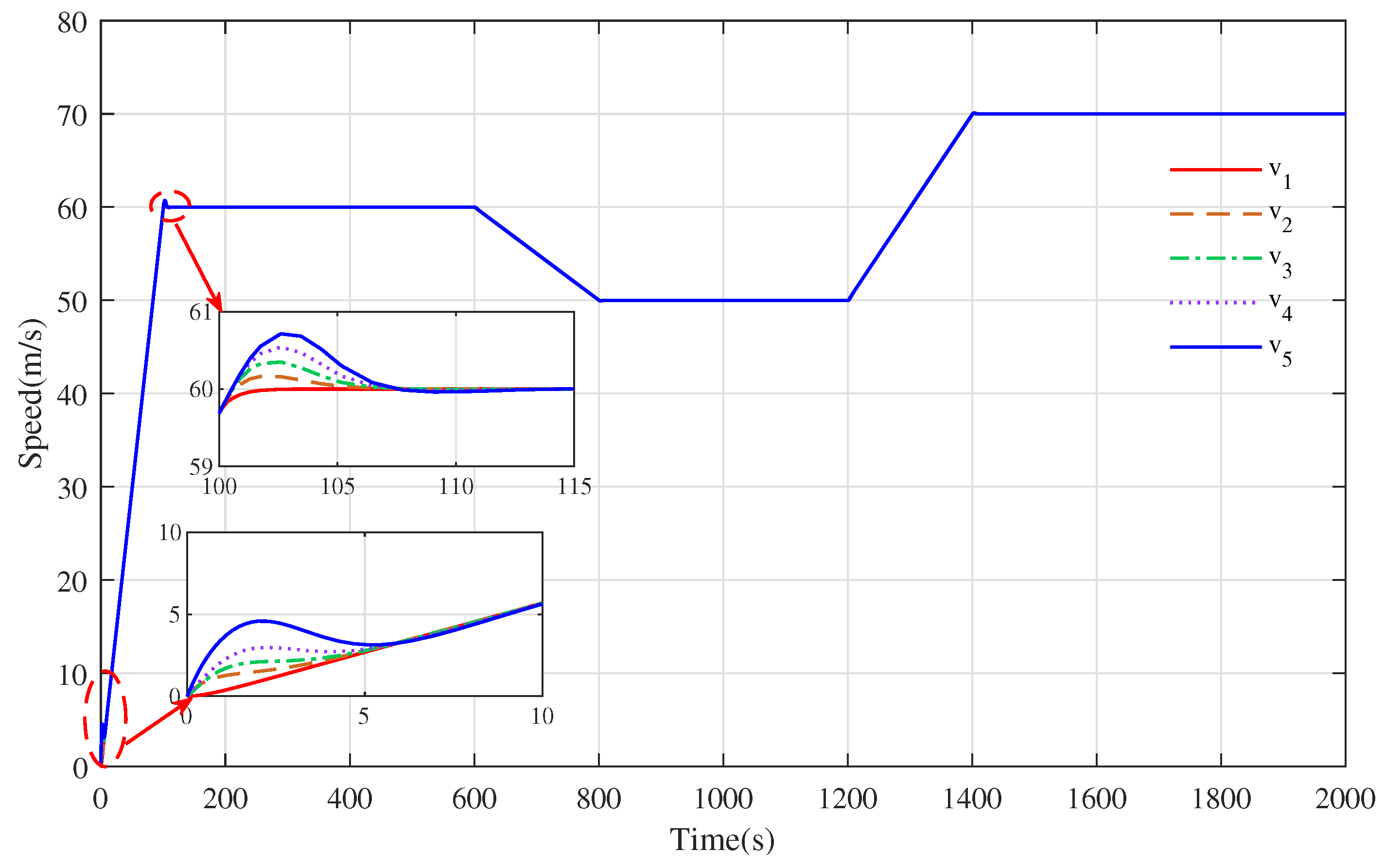
Under the action of the basic distributed cooperative strategy, the speed tracking curve and distance evolution curve of each train is shown in Figure 4 and Figure 5, respectively. It is clearly observed from Figure 4 that due to the role of in the control strategy, the speed of all the trains eventually could achieve a consensus in each operation phase, but the states’ curves trajectory fluctuated for a long time before converging to the desired speed. During the acceleration phase in s, the desired speed received by each train kept getting larger, and meanwhile the amount of information that needed to be processed by each train became larger as the state information was transmitted sequentially, which led to a large speed error, so the speed curve trajectory oscillated in the time period of s. Obviously, the unnecessary energy consumption was caused by the redundant traction and braking of each train. Moreover, please note that the amplitude of the speed curve trajectory in Figure 4 within s was too small to be observed easily. All the trains completed the first acceleration within s until 120 s to reach the desired speed 60 m/s, and they ran stably within s. At 600 s, the desired speed decreased to 50 m/s, and all trains gradually completed the deceleration within s until the desired speed was tracked to 50 m/s at 813 s and ran stably at this speed within s. At 1400 s, the desired speed increased to 70 m/s, and all trains completed acceleration within s until the desired speed 70 m/s was tracked at 1419s, and they kept operating within s. In the multiple trains’ distributed cooperative cruise control system, only the first train always communicates with the virtual leader train, and each of the rear trains only receives information from the train ahead. Therefore, the distributed cooperative cruise control can only be realized when the state information of the virtual lead train is transmitted to all trains. This also means that if the desired speed changes, the previously maintained consensus will also be broken, and a new consensus will need to be reached by retransmitting the information.
Based on the basic distributed control strategy, the distance evolution curve between the trains is shown in Figure 5. Owing to the cooperative term , the distance between the trains is calculated in real time according to the cooperative control algorithm and converges to the desired safe distance km. From Figure 5, it is observed that the oscillation of the distance evolution curve before convergence is due to the large initial state error, which is more serious within s and s. In addition, with the decrease and increase in the desired speed of s and s, respectively, the lead and lag of the rear train speed changes will also lead to the corresponding decrease or increase in the distance among the trains.
The simulation results showed that the basic cooperative control strategy can effectively avoid collisions among trains while achieving speed tracking. However, its large state error makes the trains’ tracking performance poor, and the amplitude of the speed tracking error shows frequent oscillation. This phenomenon will reduce the driving comfort and increase the energy consumption of the trains.
4.2.2. Simulation Test for the Control Strategy in Reference [7]
The speed tracking curve and distance convergence curve are shown in Figure 6 and Figure 7 under the action of the cooperative controller proposed in Reference [7]. It can be observed from Figure 6 that all the trains had a good convergence performance during the cruise phase. At s, the trains reached a consensus in 5 s, and similarly, at s and s, the trains could converge in 2 s. However, the trains could not accurately track the desired speed curve in the acceleration and deceleration phases. In the acceleration phase within s and s, the convergence speed was less than the desired speed, and in the deceleration phase within s, the train speed was greater than the desired speed. Meanwhile, because the control strategy proposed in [7] requires that each train can receive the speed information of the virtual leader train, when all trains achieve a consensus for the first time in about 30 s, the distance between the adjacent trains will always be stable at km and will not change because of the change in the desired speed. The results showed that the high-speed train could converge to the cooperative state by using the control strategy in reference [7], but the tracking accuracy was not high, and it could not accurately track the expected speed when the speed changed. Secondly, the train’s running state also oscillated frequently before the first convergence, which caused the train to consume more energy.
4.2.3. Simulation Test for the Optimal Distributed Cooperative Control Strategy
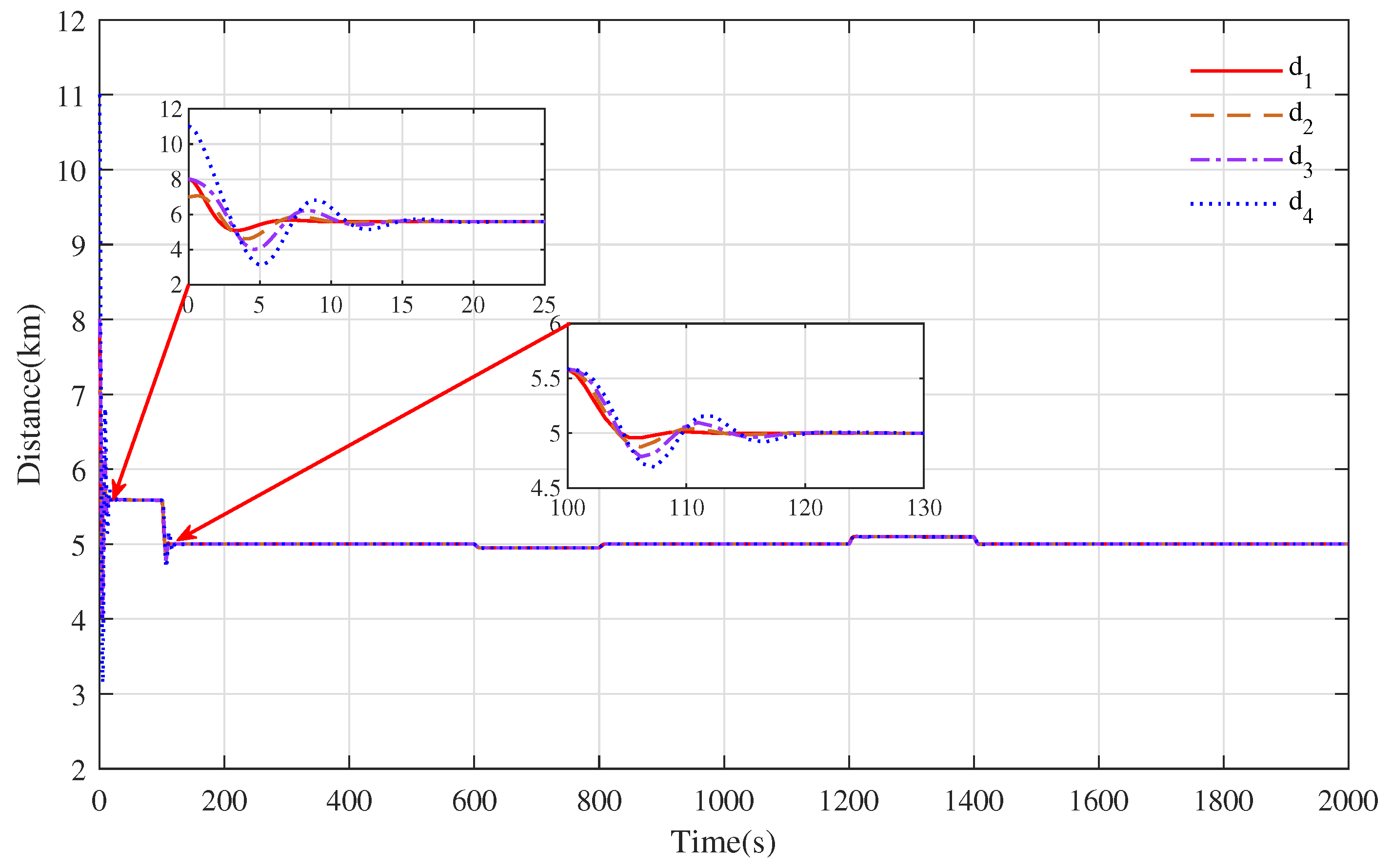
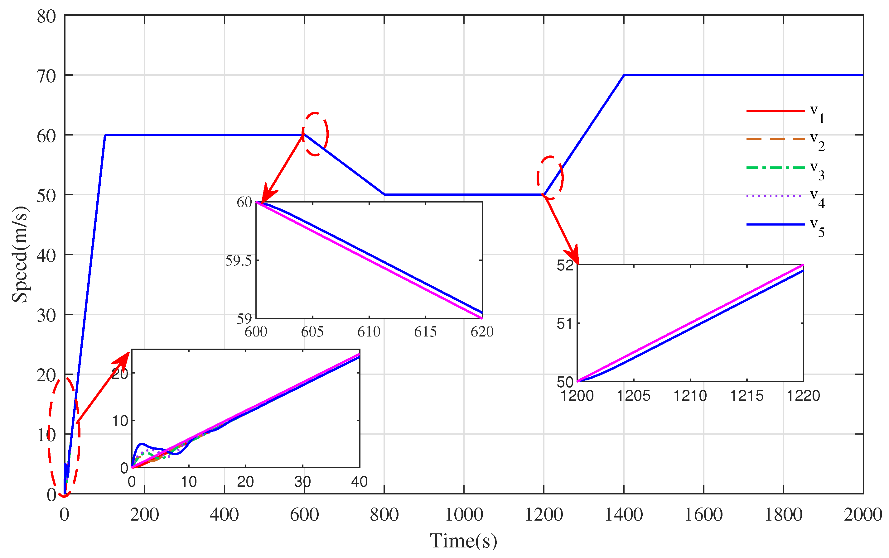
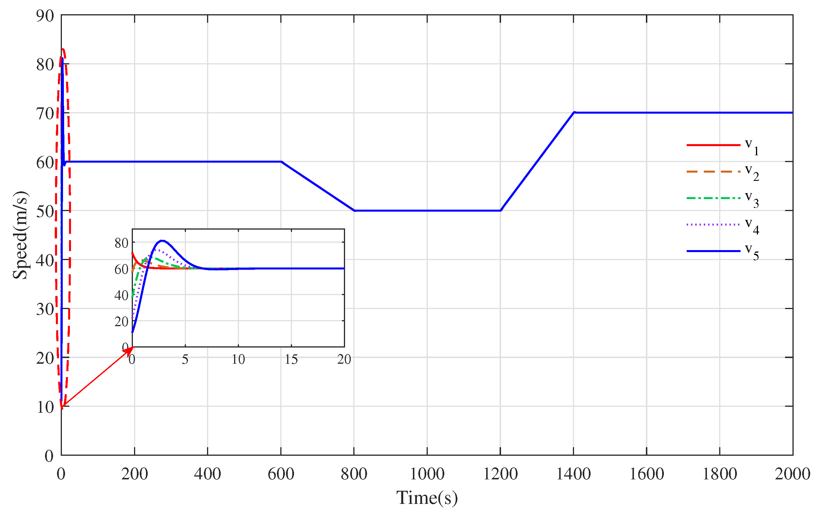
Regarding the simulation result proposed in Figure 4, Figure 5, Figure 6 and Figure 7, we observed that although each train could achieve a speed consensus while keeping a safe distance among the trains, the curves’ convergence process fluctuated greatly, which causes the multiple trains’ cruise control system to have the disadvantages of having a large overshoot, more energy consumption and poor running comfort. To improve these drawbacks, we applied the design technique to decrease the state errors by choosing the appropriate weight matrices and so that each train state tracking curve converges smoothly and quickly and meanwhile obtains the appropriate cooperative control gain to improve the operation efficiency and achieve energy-saving optimization. For the optimal cooperative control gain, we used provided by Equation (16) with and and chose the scalar coupling gain as as per Equation (19). By applying them to the distributed cooperative control strategy (4), the new speed tracking curves and the distance evolution curves were obtained and are shown in Figure 8 and Figure 9, respectively.
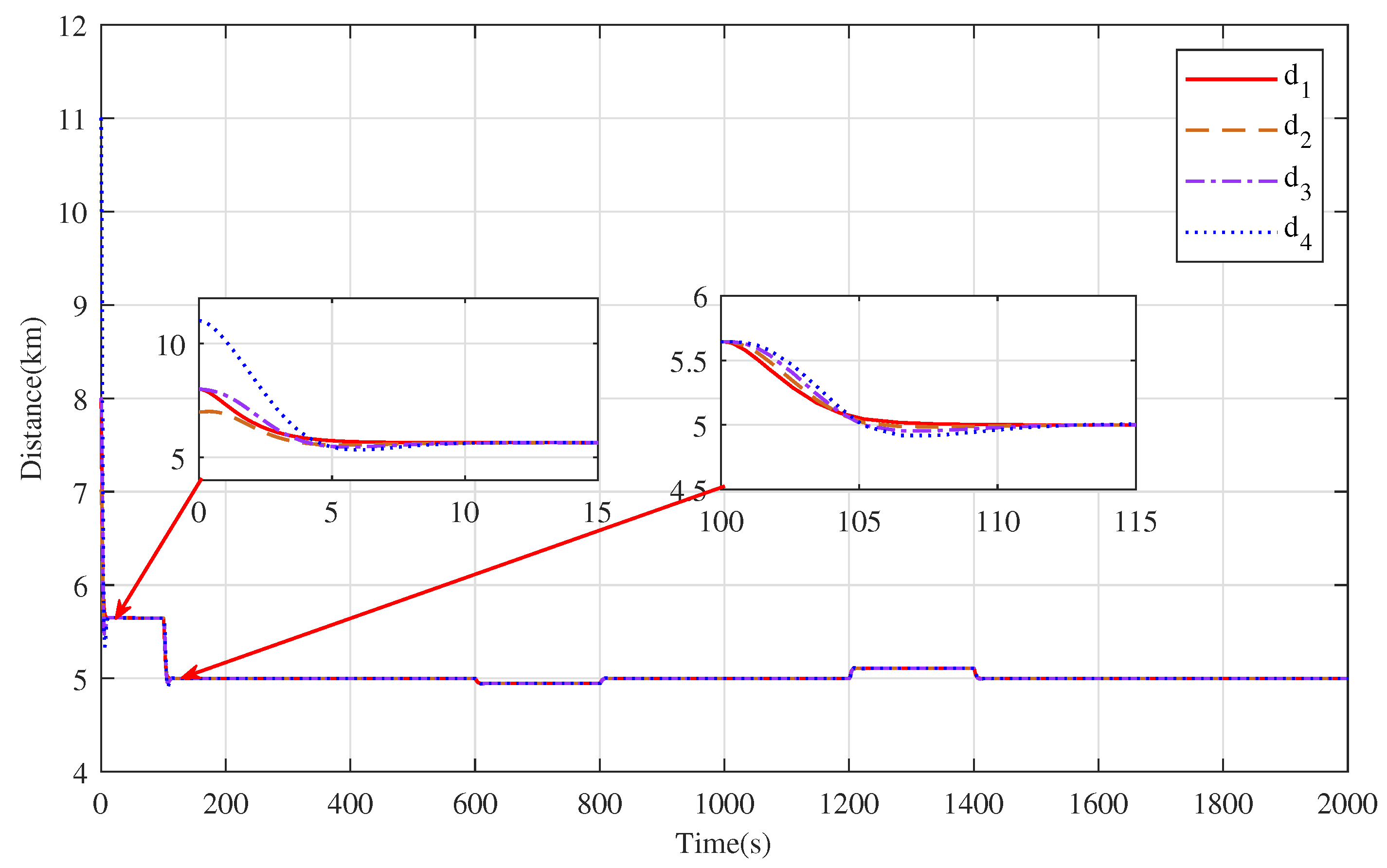
By comparing Figure 8 with Figure 4, the speed evolution curve of the train in Figure 4 showed an obvious oscillation when the speed changed, while Figure 6 was relatively flat. The speed curves of all the trains in Figure 8 converged to the desired acceleration curve trajectory at about 10 s in s, and it also only took about 12 s to track the desired speed of 60 m/s after the acceleration was completing, which was 13 s and 8 s faster than the curve convergence speed in Figure 4. This means that the speed tracking curves of the optimal distributed cooperative control strategy had less fluctuation and a faster convergence time than the basic distributed cooperative control strategy, which could track the virtual leader train curve trajectory faster. Comparing Figure 8 with Figure 6, the speed curves of all the trains in Figure 8 converged to the desired acceleration curve faster than that of the trains shown in Figure 6 within s, and the the virtual leader train curve trajectory could be tracked accurately in each acceleration and deceleration phase. Although the convergence time in the cruise stage was slower than that in Figure 6, the time spent was within a suitable tolerable range. From Figure 5 and Figure 9, it can be known that the distance curve changed with the speed curve. When the trains track the desired speed, the safety distance between the trains will achieve a consensus. Because the optimization technique is adopted to reduce the state errors, the distance curve trajectories in Figure 9 are very smooth, and the convergence speed is fast. It only takes about 112 s, 211 s and 216 s to maintain the desired safe distance among the trains in s, s and s, while in Figure 5, 120 s, 213 s and 219 s are required, respectively.
The simulation results showed that the time can be shortened to achieve cooperative control and consume less energy at each operation phase based on the proposed optimal distributed cooperative control strategy.
4.3. Simulation Test for Performance Indexes Comparison under These Three Control Strategies
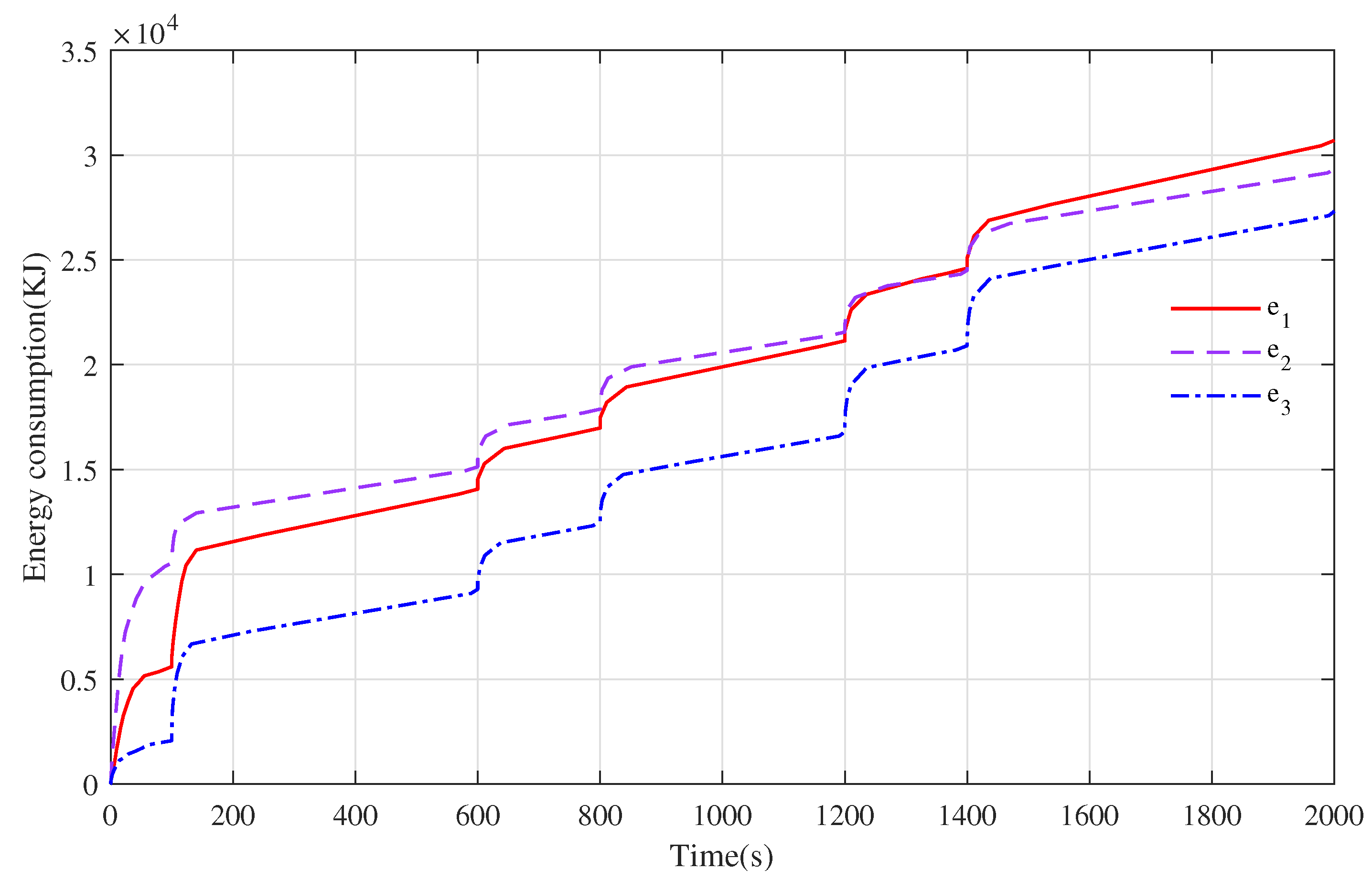
In this paper, two performance indexes (energy consumption and convergence time) were selected to compare these three different control strategies. The energy consumption curves are shown in Figure 10, and the energy consumption of our proposed strategy was apparently lower than the basic cooperative control strategy. Since the convergence performance of all the trains were nearly similar with each phase, the acceleration phase s and cruising phase s were selected for the comparison of the convergence times. The specific comparison results are shown in Table 2. The convergence times of the three different control strategies in the first acceleration phase were 23 s, 30 s and 10 s respectively. The first time that the three different control strategies converged to the desired speed was 120 s, 105 s and 112 s in the cruising phase, respectively.
Aiming at the energy consumption problem of the train tracking operation, the basic cooperative control strategy and the control strategy proposed in reference [7] oscillates strongly during the acceleration phase and when it converges to the desired speed for the first time. Although it can maintain a good cooperative performance eventually, the shock caused by the control input will lead to more actions of internal actuators that consume more energy than the optimal distributed cooperative control strategy proposed in this paper. The optimal distributed cooperative control and the optimal control for each train both experience the cooperative control gain when the appropriate weight matrix is chosen to obtain a flexible control strategy, which thus improves the train operation performance. In general, the optimal distributed cooperative control strategy saved and energy consumption compared with the basic cooperative control strategy and the control strategy in reference [7].
4.4. Simulation Test of Consensus Ability of Optimal Distributed Cooperative Control Strategy under Nonzero Initial Speed
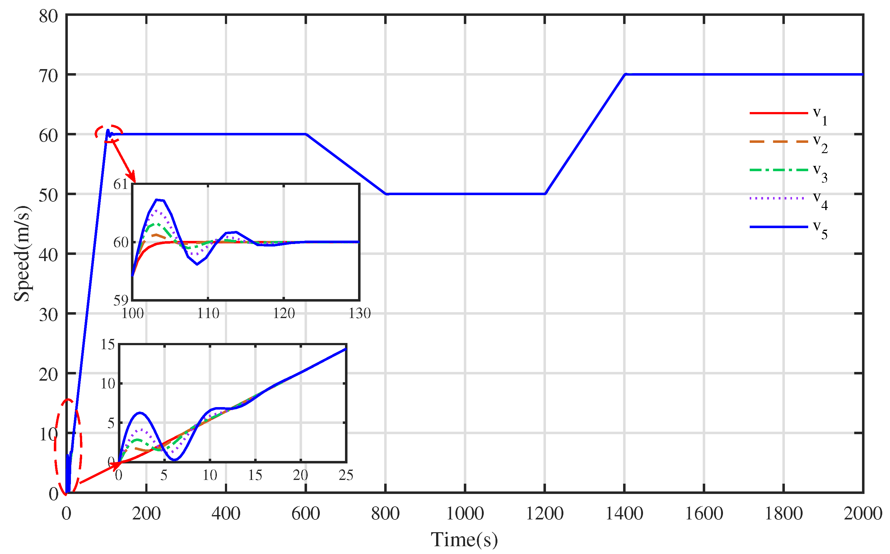
In this section, we give the initial position and speed and the virtual lead train speed curve trajectory again, as shown in Table 3 and Figure 11, respectively.
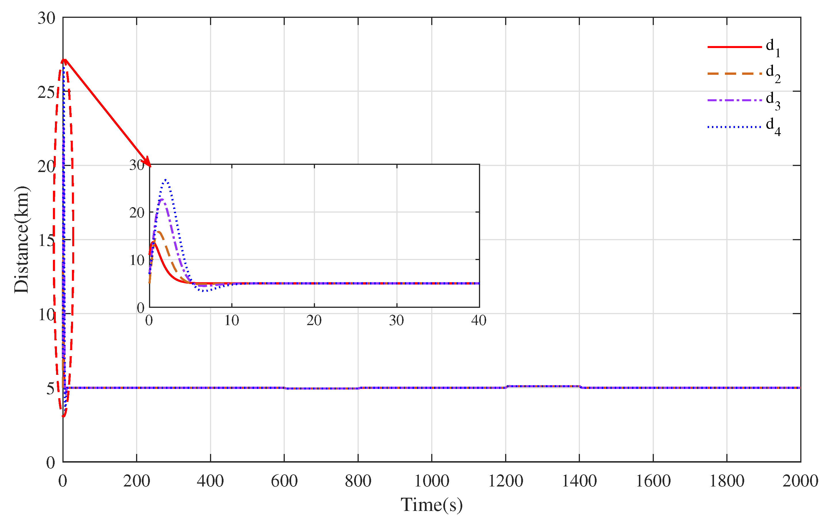
Based on the optimal distributed cooperative control strategy, the speed tracking curve and distance evolution curve of each train at a nonzero initial speed are shown in Figure 12 and Figure 13, respectively. As shown in Figure 12, the trains with different initial speeds could track the desired speed curve with a good tracking performance and excellent control effect of rapidity and accuracy. During the whole tracking operation, due to the large difference in the initial speeds, it took more time for all the trains to achieve consensus within [0,100] s than in the following phases, and the speeds of all the trains were aligned after about 12 s of information transmission. In the following operation phases, the consensus of each train did not change obviously due to the change in speed. Moreover, the distance curves between the trains are constantly changing with the change in the train speed in Figure 13. When all the trains reach a consensus, all the distance curves are kept at a given distance value, and during the whole simulation process, all the trains keep a safe distance. The simulation results fully demonstrated the consensus ability of the optimal distributed cooperative control strategy, which means that the control strategy could be used to solve additional problems regarding multiple trains’ cooperative cruise control at different initial speeds.
5. Conclusions
In this paper, the problem of optimal distributed cooperative cruise control for multiple trains is studied. An optimal distributed cooperative control method based on is proposed to achieve the displacement and speed consensus of all trains with energy-saving optimization. The cooperative control gain was obtained by using optimization to minimize the relative state errors and energy consumption during the cooperative operation of multiple trains. Moreover, the proposed strategy is robust when it comes to arbitrary directed communication topologies with a sufficient condition for the scalar coupling gain. The stability of the system was proved by the Hurwitz and Lyapunov stability theorem. The feasibility of the designed optimal cooperative control algorithm was verified by comparing the energy consumption of the basic cooperative control algorithm through a simulation. Additionally, the comfort of the train during the distributed cruise and the delay in the communication network were not considered, which will be investigated in the future.
Author Contributions
Conceptualization, F.Z. and K.T.; methodology, F.Z., K.T. and B.C.; software, K.T. and B.C.; validation, F.Z., B.C. and Z.Z.; formal analysis, Y.Y. and B.C.; investigation, K.T.; resources, F.Z.; data curation, S.L.; writing—original draft preparation, K.T.; writing—review and editing, F.Z. and B.C.; visualization, K.T. and Y.Y.; supervision, S.L.; project administration, F.Z.; funding acquisition, F.Z., S.L. and Y.Y. All authors have read and agreed to the published version of the manuscript.
Funding
The authors would like to acknowledge that this work was partially supported by the National Natural Science Foundation of China (Grant No. 61502055), Changsha Municipal Natural Science Foundation (Grant No. 2021cskj014), the General project of Hunan Natural Science Foundation (Grant No. 2021JJ30876) and the Research Foundation of Education Bureau of Hunan Province, China (Grant No. 21B0303).
Institutional Review Board Statement
Not applicable.
Informed Consent Statement
Not applicable.
Data Availability Statement
Not applicable.
Conflicts of Interest
The authors declare no conflict of interest.
Notation
The symbol ⊗ is used to represent the Kronecker product. is used to represent an identity matrix of n. denotes a - dimensional matrix with all components being equal to 0. The superscript T is the transpose of the matrices. The superscript H is the conjugate transpose of the matrices.
References
- Xun, J.; Yin, J.; Liu, R.; Liu, F.; Zhou, Y.; Tang, T. Cooperative control of high-speed trains for headway regulation: A self-triggered model predictive control based approach. Transp. Res. Part C: Emerg. Technol. 2019, 102, 106–120. [Google Scholar] [CrossRef]
- Bai, W.; Dong, H.; Zhang, Z.; Li, Y. Coordinated Time-Varying Low Gain Feedback Control of High-Speed Trains Under a Delayed Communication Network. IEEE Trans. Intell. Transp. Syst. 2022, 23, 4331–4341. [Google Scholar] [CrossRef]
- Wang, X.; Liu, L.; Zhu, L.; Tang, T. Train-Centric CBTC Meets Age of Information in Train-to-Train Communications. IEEE Trans. Intell. Transp. Syst. 2020, 21, 4072–4085. [Google Scholar] [CrossRef]
- Dong, H.; Gao, S.; Ning, B. Cooperative Control Synthesis and Stability Analysis of Multiple Trains Under Moving Signaling Systems. IEEE Trans. Intell. Transp. Syst. 2016, 17, 2730–2738. [Google Scholar] [CrossRef]
- Ning, B.; Dong, H.; Gao, S. Distributed cooperative control of multiple high-speed trains under a moving block system by nonlinear mapping-based feedback. Sci. China 2018, 61, 1–12. [Google Scholar] [CrossRef]
- Li, S.; Yang, L.; Gao, Z. Adaptive coordinated control of multiple high-speed trains with input saturation. Nonlinear Dyn. 2016, 83, 2157–2169. [Google Scholar] [CrossRef]
- Lin, P.; Huang, Y.; Zhang, Q.; Yuan, Z. Distributed Velocity and Input Constrained Tracking Control of High-Speed Train Systems. IEEE Trans. Syst. Man, Cybern. Syst. 2021, 51, 7882–7888. [Google Scholar] [CrossRef]
- Gao, S.; Dong, H.; Ning, B.; Qi, Z. Cooperative Prescribed Performance Tracking Control for Multiple High-Speed Trains in Moving Block Signaling System. IEEE Trans. Intell. Transp. Syst. 2019, 20, 2740–2749. [Google Scholar] [CrossRef]
- Huang, Z.; Wang, P.; Zhou, F.; Liu, W.; Peng, J. Cooperative Tracking Control of the Multiple-High-Speed Trains System Using a Tunable Artificial Potential Function. J. Adv. Transp. 2022, 2022, 3639586. [Google Scholar] [CrossRef]
- Bilgen, S.; Sarıkaya, İ. Energy conservation policy and environment for a clean and sustainable energy future. Energy Sources Part B Econ. Plan. Policy 2018, 13, 183–189. [Google Scholar] [CrossRef]
- Su, S.; Tang, T.; Roberts, C. An explicit nonlinear model predictive ABS controller for electro-hydraulic braking systems. IEEE Trans. Intell. Transp. Syst. 2015, 16, 622–631. [Google Scholar] [CrossRef]
- Huang, Y.; Yu, H.; Yin, J.; Hu, H.; Bai, S.; Meng, X.; Wang, M. An integrated approach for the energy-efficient driving strategy optimization of multiple trains by considering regenerative braking. Comput. Ind. Eng. 2018, 126, 399–409. [Google Scholar] [CrossRef]
- Chen, M.; Xiao, Z.; Sun, P.; Wang, Q.; Jin, B.; Feng, X. Energy-Efficient Driving Strategies for Multi-Train by Optimization and Update Speed Profiles Considering Transmission Losses of Regenerative Energy. Energies 2019, 12, 3573. [Google Scholar] [CrossRef]
- Su, S.; Wang, X.; Cao, Y.; Yin, J. An Energy-Efficient Train Operation Approach by Integrating the Metro Timetabling and Eco-Driving. IEEE Trans. Intell. Transp. Syst. 2020, 21, 4252–4268. [Google Scholar] [CrossRef]
- Chou, M.; Xia, X. Optimal cruise control of heavy-haul trains equipped with electronically controlled pneumatic brake systems. Control Eng. Pract. 2007, 15, 511–519. [Google Scholar] [CrossRef]
- Zhang, R.; Peng, J.; Liu, W.; Chen, B.; Wang, J. A Consensus Control with Application to Heavy Haul Trains Based on Switched Hierarchical LQR. In Proceedings of the 2016 International Conference on Collaboration Technologies and Systems (CTS), Orlando, FL, USA, 31 October–4 November 2016; pp. 322–348. [Google Scholar]
- Boukadida, W.; Benamor, A.; Messaoud, H.; Siarry, P. Multi-objective design of optimal higher order sliding mode control for robust tracking of 2-DoF helicopter system based on metaheuristics. Aerosp. Sci. Technol. 2019, 91, 442–455. [Google Scholar] [CrossRef]
- Zhang, F.; Zhang, H.; Tan, C.; Wang, W.; Gao, J. A new approach to distributed control for multi-agent systems based on approximate upper and lower bounds. Int. J. Control. Autom. Syst. 2017, 15, 2507–2515. [Google Scholar] [CrossRef]
- Zhang, H.; Lewis, F.L.; Das, A. Optimal Design for Synchronization of Cooperative Systems: State Feedback, Observer and Output Feedback. IEEE Trans. Autom. Control 2011, 56, 1948–1952. [Google Scholar] [CrossRef]
- Tomic, I.; Halikias, G.D. Performance analysis of distributed control configurations in LQR multi-agent system design. In Proceedings of the 2016 UKACC 11th International Conference on Control (CONTROL), Belfast, UK, 31 August–2 September 2016. [Google Scholar]
- Bai, W.; Lin, Z.; Dong, H. Coordinated Control in the Presence of Actuator Saturation for Multiple High-Speed Trains in the Moving Block Signaling System Mode. IEEE Trans. Veh. Technol. 2020, 69, 8054–8064. [Google Scholar] [CrossRef]
- Wang, X.; Zhu, L.; Wang, H.; Tang, T.; Li, K. Robust Distributed Cruise Control of Multiple High-Speed Trains Based on Disturbance Observer. IEEE Trans. Intell. Transp. Syst. 2021, 22, 267–279. [Google Scholar] [CrossRef]
- Xu, X.; Peng, J.; Zhang, R.; Chen, B.; Huang, Z. Adaptive Model Predictive Control for Cruise Control of High-Speed Trains with Time-Varying Parameters. J. Adv. Transp. 2019, 2019, 1–11. [Google Scholar] [CrossRef]
- Li, S.; Yang, L.; Gao, Z. Coordinated cruise control for high-speed train movements based on a multi-agent model. Transp. Res. Part C 2015, 56, 281–292. [Google Scholar] [CrossRef]
- Zhou, F.; Huang, Z.; Gao, K.; Li, L.; Liao, H.; Peng, J. Distributed cooperative tracking control for heavy haul trains with event-triggered strategy. In Proceedings of the 2016 American Control Conference (ACC), Boston, MA, USA, 6–8 July 2016. [Google Scholar]
- Lian, B.; Lewis, F.L.; Hewer, G.A.; Estabridis, K.; Chai, T. Online Learning of Minmax Solutions for Distributed Estimation and Tracking Control of Sensor Networks in Graphical Games. IEEE Trans. Control Netw. Syst. 2022, 9, 1923–1936. [Google Scholar] [CrossRef]
- Li, S.K.; Yang, L.X.; Li, K.P. Robust output feedback cruise control for high-speed train movement with uncertain parameters*. Chin. Phys. B 2015, 24, 010503. [Google Scholar] [CrossRef]
Figure 1.
The diagram of n trains cooperative movement.

Figure 2.
Simplified control architecture of the proposed strategy.

Figure 3.
The speed trajectory of virtual leader train. It is clearly observed from Figure 3 that s and s are acceleration phases. s, s and s are cruising phases which operate at 60 m/s, 50 m/s and 70 m/s, respectively. s is deceleration phase.
Figure 3.
The speed trajectory of virtual leader train. It is clearly observed from Figure 3 that s and s are acceleration phases. s, s and s are cruising phases which operate at 60 m/s, 50 m/s and 70 m/s, respectively. s is deceleration phase.

Figure 4.
The speed tracking curve trajectory by applying basic distributed cooperative control strategy.
Figure 4.
The speed tracking curve trajectory by applying basic distributed cooperative control strategy.

Figure 5.
The tracking distance evolution curve between trains by applying basic distributed cooperative control strategy.
Figure 5.
The tracking distance evolution curve between trains by applying basic distributed cooperative control strategy.

Figure 6.
The speed tracking curve under the action of the proposed cooperative controller based on reference [7].
Figure 6.
The speed tracking curve under the action of the proposed cooperative controller based on reference [7].

Figure 7.
The tracking distance evolution curve between trains under the action of the proposed cooperative controller based on reference [7].
Figure 7.
The tracking distance evolution curve between trains under the action of the proposed cooperative controller based on reference [7].

Figure 8.
The speed tracking curve trajectory by applying optimal distributed cooperative control strategy.
Figure 8.
The speed tracking curve trajectory by applying optimal distributed cooperative control strategy.

Figure 9.
The tracking distance evolution curve between trains by applying optimal distributed cooperative control strategy.
Figure 9.
The tracking distance evolution curve between trains by applying optimal distributed cooperative control strategy.

Figure 10.
The trajectory diagram of the energy consumption curve under three different control strategies, where refers to the basic cooperative control strategy, refers to the cooperative control strategy in reference [7] and refers to the optimal distributed cooperative control strategy.
Figure 10.
The trajectory diagram of the energy consumption curve under three different control strategies, where refers to the basic cooperative control strategy, refers to the cooperative control strategy in reference [7] and refers to the optimal distributed cooperative control strategy.

Figure 11.
The speed curve trajectory of virtual leader train.

Figure 12.
The speed tracking curve trajectory by applying optimal distributed cooperative control strategy.
Figure 12.
The speed tracking curve trajectory by applying optimal distributed cooperative control strategy.

Figure 13.
The tracking distance evolution curve between trains by applying optimal distributed cooperative control strategy.
Figure 13.
The tracking distance evolution curve between trains by applying optimal distributed cooperative control strategy.


Table 1.
The initial speeds and positions of each high-speed train.
| i | 1 | 2 | 3 | 4 | 5 |
|---|---|---|---|---|---|
| 57 km | 49 km | 42 km | 34 km | 23 km | |
| 0 m/s | 0 m/s | 0 m/s | 0 m/s | 0 m/s |
Table 2.
Three different control strategies are compared from the perspectives of convergence time and energy consumption.
Table 2.
Three different control strategies are compared from the perspectives of convergence time and energy consumption.
| Convergence Time within Acceleration Phase [0,100] s | Convergence Time within Cruising Phase [100,600] s | Energy Consumption | |
|---|---|---|---|
| The basic distributed cooperative control | 23 s | 20 s | KJ |
| The cooperative control in reference [7] | 30 s | 5 s | KJ |
| The optimal distributed cooperative control | 10 s | 12 s | KJ |
Table 3.
The initial speeds and positions of each high-speed train.
| i | 1 | 2 | 3 | 4 | 5 |
|---|---|---|---|---|---|
| 64 km | 53 km | 48 km | 41 km | 34 km | |
| 72 m/s | 57 m/s | 38 m/s | 22 m/s | 11 m/s |
Disclaimer/Publisher’s Note: The statements, opinions and data contained in all publications are solely those of the individual author(s) and contributor(s) and not of MDPI and/or the editor(s). MDPI and/or the editor(s) disclaim responsibility for any injury to people or property resulting from any ideas, methods, instructions or products referred to in the content. |
© 2023 by the authors. Licensee MDPI, Basel, Switzerland. This article is an open access article distributed under the terms and conditions of the Creative Commons Attribution (CC BY) license (https://creativecommons.org/licenses/by/4.0/).
Share and Cite
MDPI and ACS Style
Zhou, F.; Tao, K.; Chen, B.; Li, S.; Zhu, Z.; Yang, Y. Distributed Cooperative Cruise Control for High-Speed Trains with Energy-Saving Optimization. Actuators 2023, 12, 207. https://doi.org/10.3390/act12050207
AMA Style
Zhou F, Tao K, Chen B, Li S, Zhu Z, Yang Y. Distributed Cooperative Cruise Control for High-Speed Trains with Energy-Saving Optimization. Actuators. 2023; 12(5):207. https://doi.org/10.3390/act12050207
Chicago/Turabian StyleZhou, Feng, Kewu Tao, Bin Chen, Shuo Li, Zhengfa Zhu, and Yingze Yang. 2023. "Distributed Cooperative Cruise Control for High-Speed Trains with Energy-Saving Optimization" Actuators 12, no. 5: 207. https://doi.org/10.3390/act12050207
Note that from the first issue of 2016, this journal uses article numbers instead of page numbers. See further details here.