Article

Uncalibrated Adaptive Visual Servoing of Robotic Manipulators with Uncertainties in Kinematics and Dynamics

1
School of Automation, Guangdong University of Technology, Guangzhou 510006, China
2
School of Mechanical and Electrical Engineering, Guangzhou City Polytechnic, Guangzhou 510405, China
3
Concordia Wisconsin Campus, Concordia University, 12800 N Lake Shore Drive, Mequon, WI 53097, USA
*
Authors to whom correspondence should be addressed.
Actuators 2023, 12(4), 143; https://doi.org/10.3390/act12040143
Submission received: 8 February 2023 / Revised: 10 March 2023 / Accepted: 23 March 2023 / Published: 27 March 2023
(This article belongs to the Special Issue Advanced Technologies and Applications in Robotics)

Abstract

:
In the study, we propose a novel adaptive visual servoing control scheme for robotic manipulators with kinematic and dynamic uncertainties, where the camera used is uncalibrated, which implies that its intrinsic and extrinsic parameters are unavailable for measurement. For our scheme, a depth-independent composite Jacobian matrix is constructed to make visual parameters and robotic physical parameters appear linearly in a parametrized uniform form so that an adaptive algorithm can be developed to estimate their values. With the raised adaptive algorithm, the potential singularity of the Jacobian matrix can be well circumvented by updating estimated parameters in an appropriate tiny range of actual values. With our scheme, the asymptotic convergence of the image tracking error to zero is established successfully, in addition to the signal boundedness of the closed-loop system. The effectiveness of the proposed scheme is confirmed by simulation results based on a 6-DOF PUMA manipulator.

1. Introduction

The control scheme of robotic manipulators is always a hot topic in research for its wide application in various industries [1,2,3,4,5,6,7,8]. With the development of information technology, visual sensors are widely used in the control system of the robotic manipulator to deal with complex and volatile tasks. In [1], the traditional visual feedback control approach is proposed for an assembling robotic manipulator. Specifically, the traditional visual feedback system adopts a look-and-move approach, which separates the image process from the controller of a manipulator to make the control structure hierarchical [5]. The visual servo originated from [4], which is a vision-based controller constructed to drive the motor of a manipulator directly. Lots of visual servoing control approach for a robotic manipulator have been proposed, such as [6,9,10,11,12,13], in recent decades.
To categorize diverse visual servoing architectures, many taxonomies (the number of cameras, the configuration of vision systems, and the space where error functions are defined) are proposed [6]. Generally, the visual servoing control can be categorized into subsequent two approaches according to the definition of its error function. One is the Position-Based Visual Servoing (PBVS) control scheme, whose error function is defined in a task space by the difference between the current position (estimated by visual information) and the desired position of a manipulator [11]. The control accuracy of the PBVS control scheme is subject to the precise estimation of a robotic position, which is dependent on the calibration of the parameters in the visual servoing system. The other is the Image-Based Visual Servoing (IBVS) control scheme which directly utilizes image information to construct the error function in image space [12]. Both of the PBVS and the IBVS traditional control methods need to calibrate the system, including a vision system and a robotic manipulator system. Additionally, the performance of the visual servoing system is directly influenced by the calibration accuracy. However, parametric calibration is a tedious and highly costly task. Even a precise calibrated system would change in some harsh environments. To address this problem, the techniques of uncalibrated visual servoing for a robotic manipulator have become a popular research topic in the field of visual servoing [9,10].
The key idea of the so-called uncalibrated visual servoing method is designing a controller of a robotic manipulator by the image errors for ensuring that the system error converges to an acceptable range without the pre-calibrated system parameters (the extrinsic/intrinsic parameters of the used camera and the robotic parameters). Since the IBVS methods are more robust for the error of the control model rather than the PBVS methods substantial efforts (concerning IBVS methods) in addressing the uncertainties due to unknown or unprecise parameters have been made [13,14,15,16,17]. Generally, the design idea of an uncalibrated IBVS method features the estimation of the composite Jacobian matrix (the image matrix [14]) utilized to design the control law. The composite Jacobian matrix relates the velocity of the end-effector of a robotic manipulator in joint space to the velocity of the image features in image space. An online composite Jacobian matrix estimator based on a dynamic Kalman filter algorithm is developed in [14]. In [15,16,17], the approaches based on recursive least squares are proposed to estimate the composite Jacobian matrix online. Furthermore, Ref. [13] presents a fuzzy learning approach for an IBVS system. The above approaches are all developed based on kinematics and feature the following points: (i) a numerical method is adopted to estimate the whole Jacobian matrix without the explicit expression of a Jacobian matrix; (ii) the uncertainties in the dynamics of a robotic manipulator are neglected. However, the performance and stability of visual servoing are affected by the non-linear forces of a robotic manipulator in high-speed motion. Therefore, a vast amount of research about an IBVS method considering the nonlinear force of the robotic dynamics has been invested [18,19,20,21,22,23,24,25,26,27].
Compared to the kinematics-based control scheme, the dynamics-based control scheme mainly adopts the analytical method to figure out the linear form of unknown parameters in the explicit expression of a Jacobian matrix and then adopts the adaptive algorithm to estimate them. In [19], an approximate Jacobian control method for a planar robotic manipulator with kinematic and dynamic uncertainties is proposed. With visual servoing control for a planar robotic manipulator, the depth of the feature point relative to the camera frame is constant. However, it is worth mentioning that the depth information of an image feature appearing in the explicit Jacobian matrix is unknown and unmeasurable, and thus dealing with the uncertainties caused by the unknown depth information is a challenging problem in the dynamics-based control scheme. The direct scheme to tackle the unknown depth information is utilizing a stereo camera [20,28], which aggravates the computation complexity. Additionally, an adaptive updating algorithm for the depth information of image features is proposed in [21]. However, it is available only under the slow time-varying constraint of the depth of information. Thus, a depth-independent interaction matrix is originally presented in [22] to address the constraint of the slow time-varying for the depth information, which enables the interaction matrix parametrized by the camera parameters. Subsequently, a dynamic trajectory tracking control for uncalibrated visual servoing is extended in [23]. However, the methods in [22,23] are limited by the prior knowledge of robotic kinematics, assuming that the robotic Jacobian matrix is available for measurement. With un-precise kinematic parameters, a depth-independent image Jacobian matrix is utilized to map the image errors onto the robotic joint space in [24], where unknown parameters are estimated by an adaptive algorithm online. The work in [25] generalizes the control method in [24] from a point feature to a generalized image feature. However, the precise world coordinates of feature points adopted in [24,25] are unmeasurable in a practical case. Easy access to all the parameters and data in a controller is desired for an uncalibrated visual servoing control method. Moreover, the depth and the Jacobian matrix are individually estimated in [26,27]. Meanwhile, the uncertainties in dynamics caused by unknown robotic physical parameters, i.e., the gravitational torque of robotic manipulators, are neglected in [25,27]. In short, the kinematic and dynamic uncertainties caused by unknown parameters of the visual servoing are not or partially discussed in the above methods.
Prompted by the above studies and expanding from our previous work [29], in this paper, an IBVS scheme is presented to handle the kinematic and dynamic uncertainties (caused by the unknown parameters of the camera and the robotic manipulator) under the uncalibrated environment. The raised controller drives a robotic manipulator with uncertainties, where the feature points are marked, ensuring the projection of those points converges to the desired area in the image plane. One of the major problems that obstruct the application of the method in [22] in absence of the parameters of a robotic manipulator is the fact that the robotic Jacobian matrix can not be parameterized as a linear form together with the interaction matrix. The other problem is the gravitational torque for an uncalibrated robotic manipulator is unknown, which yields uncertainties in dynamics. To solve the former problem, a depth-independent composite Jacobian matrix and a depth Jacobian matrix are constructed, both of which can be parametrized in a uniform linear parametrized form. Therefore, the unknown parameters, including the extrinsic/intrinsic visual parameters and the robotic physical parameters, can be updated by an adaptive algorithm. However, since the physical parameters of manipulators are estimated by an adaptive algorithm, the non-singularity of the robotic Jacobian matrix or even the composite Jacobian matrix cannot be guaranteed, which leads to difficulties in the convergence of the image errors. To ensure asymptotic convergence, a novel adaptive algorithm using a combination of the Slotine-Li algorithm [30] with the parameter projection algorithm [31] is proposed. The aim of the introduction of the parameter projection algorithm is to ensure the estimated parameters converge to an appropriate tiny neighborhood of their actual values such that the adaptive composite Jacobian is non-singular. Meanwhile, to solve the latter problem, the adaptive algorithm we proposed is applied to compensate for the gravitational torque of a robotic manipulator. Since the estimated error of the robotic gravitational torque directly relates to the convergence of the image error, the parameter projection algorithm ensures that the adaptively estimated gravitational torque is always within an appropriate range of its true value. In this sense, the image error caused by the adaptive estimation of the gravitational torque can also be reduced to some extent. In summary, the study of this work has the following contributions and novelties:
  • A depth-independent composite Jacobian matrix is constructed, with which the unknown visual parameters and robotic physical parameters can be well arranged in a uniform linear form so that their uncertainties can be addressed by an adaptive estimation approach. Different from the existing works on the adaptive uncalibrated visual servoing control, e.g., [26,27], the unknown parameters of the visual servoing are updated by one adaptive law, which is capable of reducing the number of adaptive laws greatly.
  • In a whole uncalibrated environment, an adaptive visual servoing controller is proposed for robotic manipulators, considering the uncertainties in kinematics and dynamics comprehensively, which means all the data and parameters utilized in the controller can be obtained easily. Particularly, robotic physical parameters adopted in our raised controller can be obtained by an ocular estimation instead of a precise measuring in [22,23]. In addition, different form the related methods [25,27], the one raised in this paper takes the uncertain dynamics caused by the gravitational parameters into account and compensates for the gravity of robotic manipulators.
  • Apart from these, a novel adaptive estimation algorithm is raised, which is capable of avoiding the possible singularity of the estimated Jacobian matrix, and most importantly ensuring the asymptotic convergence of the image error. Compared with the related work in [22,23,24], the cartesian coordinates of feature points, acquired difficultly in a practical operation, are avoided in the raised adaptive algorithm, and the gravitational torque of robotic manipulators can be compensated well ensuring the image error asymptotically converges to zero better.
Finally, the asymptotic convergence of image errors is proved by the Lyapunov method. The effectiveness of the raised visual servoing control approach is confirmed by simulation based on a 6 degree-of-freedoms (DOFs) PUMA manipulator.
Notation 1. 
For clarity, we introduce here the rule for choosing notations in the paper, and definitions of some symbols. The bold upper and lower case letters are used to denote matrices and vectors, and the symbol ^ above or a matrix, vector, or scalar is used to denote an adaptive estimate of the counterpart. Besides, the notation 0 m × n is adopted to denote a zero matrix with m rows and n columns.

2. Background and Problem Statement

Consider the eye-to-hand visual control system presented in Figure 1, for which a pinhole camera is fixed to monitor the feature point marked on the end-effector of a robotic manipulator. For simplicity, and bringing our attention to the studied visual control problem well, the visual servoing system is assumed to satisfy the so-called field-of-view constraint (FOV) that the feature point marked on the end-effector is always within the field of view of the used camera. To establish the mathematical model of the studied visual control system, three coordinate frames are introduced: (i) the robotic base coordinate frame F B ; (ii) the vision coordinate frame F C ; (iii) the image coordinate frame F I . In general, the visual servo system is composed of two subsystems, as presented below.

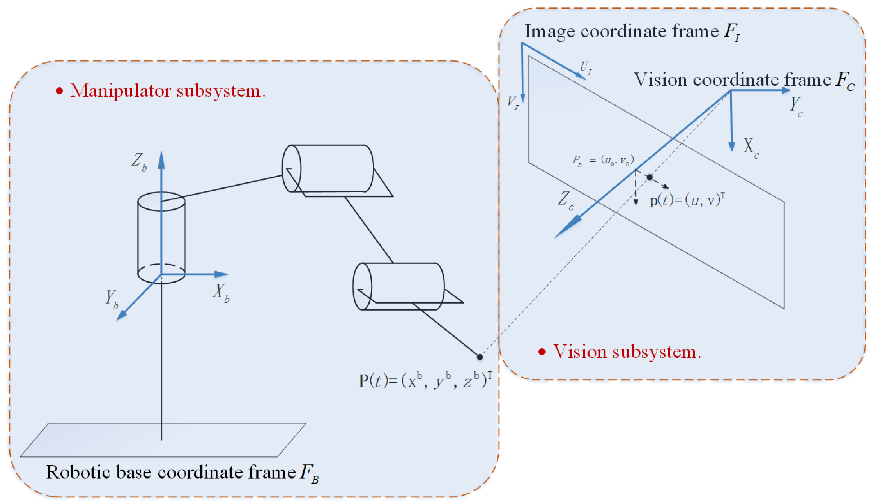
2.1. Perspective Projection Model

The process of the projection of a point from Euclidean space to image space amounts to transforming its coordinate from F B to F I . As shown in Figure 1, let us consider a feature point P marked on the end-effector of a manipulator, whose coordinate mapping relationship between F B and F C can be given by
P C 1 = T P B 1 ,
where the homogeneous transform matrix, T R 4 × 4 , represents the relationship of the rotation and translation between F B and F C . Consider the projection of P on the image plane labeled by p , whose homogeneous image coordinate is given by y = p T 1 T . Furthermore, the coordinate mapping relationship between F I and F C can be represented by the perspective projection model as follows
y = 1 z c Ω P C 1 ,
where z c represents the depth of the feature point marked on the end-effector of a manipulator relative to the origin of the vision frame F C , the matrix Ω R 3 × 4 is composed of the intrinsic parameter of a camera, whose form can be represented as
Ω = β x β x ϕ 1 u 0 0 0 β y ϕ 2 v 0 0 0 0 1 0 ,
where β x and β y are the normalized focal lengths with respect to the U I and V I axes of the image coordinate frame F I , respectively, and the ϕ i , i = 1 , 2 are the parameters determined by the nonlinear distortion of a camera. As shown in Figure 1, the Z C axis of F C is coincident with the camera optical axis and meanwhile intersects the image plane vertically at the principle point of a camera P p = ( u 0 , v 0 ) . It should be noted that the matrices determined by the extrinsic and intrinsic parameters of the camera model are constant and unknown. To estimate them with an adaptive approach, a perspective projection matrix Ξ R 3 × 4 is defined as follows
Ξ = Ω T = ξ 11 ξ 14 ξ 31 ξ 34 .
It then follows from (1), (2), and (4) that
y = 1 z c Ξ P B 1 = 1 z c Ξ x ,
where x R 4 × 1 is the homogeneous coordinate of P with respect to F B , and the depth z c in (5) have the following form:
z c = ξ 3 T x .
Here ξ 3 T represents the third row of Ξ . Observing from the perspective projection model in (5) and (6), the image coordinate, y , is the output of the system and the homogeneous coordinate, x , is the input of the model which can be accessed indirectly. Thus, the precision of the perspective projection model can be ensured when the perspective projection matrix, Ξ , is precise and accessible.
Remark 1. 
For a control model with some uncertainties due to the unknown parameters such as (5), it is commonly practiced to utilize the adaptive algorithm to construct an estimator of the unknown parameters in a controller [32,33]. Once we obtain the mapping model of the visual servo shown in Figure 1, it seems that the most reasonable control scheme is to incorporate the adaptive algorithm into the general control approaches of the robotic manipulator. However, z c , the depth of P relative to the optical point of the camera, is absent in single-camera vision. Furthermore, the depth information is inversely proportional to the perspective projection matrix so it is hard to estimate coupled with other unknown visual parameters directly. Therefore, the form of the depth in (6) is beneficial to the estimation of the unknown visual parameters in absence of the depth information.

2.2. Kinematics and Dynamics Model of Robotic Manipulator

For the robotic manipulator, the task of its kinematics analysis is to handle the mapping relationship between the work space and the joint space, and the task of its dynamics analysis is to construct the bridge from the desired joint positions/velocities to the desired joint torque. Thus, this section will is divided into two parts: one is the kinematics model, and one is the dynamics model.

2.2.1. Kinematics Model

Differentiating the nonlinear mapping between the work space and joint space x = f ( q ) in time, we obtain the well-known forward kinematics equation as follows
x ˙ = J ( q ) q ˙ ,
where q R n × 1 represents the joint position of the n-degree-of-freedom manipulator, and J ( q ) R n × n denotes the robotic Jacobian matrix. It is more desirable to obtain the relationship of the joint-space velocities relative to the image-space one rather than relative to the work-space one. Thus, differentiating (5) in time, we obtain the mapping from the work-space velocities to the image-space velocities as follows
d d t y = 1 z c Ξ x ˙ y z ˙ c = 1 z c Λ ( y ) x ˙ ,
where Λ ( y ) R 3 × 4 , named the depth-independent interaction matrix [22], can be represented as
Λ ( y ) = Ξ y ξ 3 T = ξ 1 T u ξ 3 T ξ 2 T v ξ 3 T 0 1 × 4 .
Substituting (7) into (8) yields that
d d t y = 1 z c Λ ( y ) J ( q ) q ˙ .
As the kinematics parameters of a robotic manipulator are unknown in an uncalibrated environment, the Jacobian matrix J ( q ) , including the kinematics parameters and the state variables of the manipulator, is required to be parametrized and then estimated in the control scheme. To facilitate the parametrization, construct an auxiliary matrix, i.e.,
Λ J ( q , y ) = Λ ( y ) J ( q ) = ξ 1 T j 1 u ξ 3 T j 1 ξ 1 T j 2 u ξ 3 T j 2 ξ 1 T j 3 u ξ 3 T j 3 ξ 2 T j 1 v ξ 3 T j 1 ξ 2 T j 2 v ξ 3 T j 2 ξ 2 T j 3 v ξ 3 T j 3 0 0 0 ,
where j i denotes the ith column of J ( q ) and Λ J ( q , y ) is different with the composite Jacobian matrix 1 z c Λ J ( q , y ) from Equation (10) in depth, which is named the depth-independent composite Jacobian matrix.
Remark 2. 
For the depth-independent interaction matrix frame proposed in [22], the Jacobian matrix is utilized in the controller as prior knowledge so that only the components of Ξ need to be estimated. Since the components of Ξ appear linearly in Λ ( y ) , it is easy to parametrize Λ ( y ) . However, the above linear case of the estimated parameters does not appear in parametrization when the estimated parameters involve the unknown kinematics parameters. Furthermore, it is extremely complicated to estimate the matrix Λ ( y ) and the Jacobian matrix separately by the adaptive algorithm because they include the unknown parameters and system state variables simultaneously. Therefore, introduce the depth-independent composite Jacobian matrix such as (11) to couple the unknown visual parameters with the unknown kinematics parameters and then extract them from the state variables.
Similarly, differentiating (6) in time, and incorporating with (7) yields that
z ˙ c = ξ 3 T J ( q ) q ˙ .
Similar to the (10), the unknown kinematics parameters in Jacobian matrix J ( q ) coupled with the visual parameters in the perspective projection matrix are proportional to the velocity of the depth in (12). For the sake of the formulation of the uniform parametrized form relative to Λ J ( q , y ) , the (12) can be given the following form by
z ˙ c = λ j ( q ) q ˙ ,
where λ j ( q ) is defined as
λ j ( q ) = ξ 3 T J ( q ) = ξ 3 T j 1 ξ 3 T j 2 ξ 3 T j 3 .
Remark 3. 
As λ j shown in (13) reflects the influence of the depth transform velocity of the feature point by the joint-space velocity of a manipulator, we call it the depth Jacobian matrix. The depth Jacobian matrix in (14) is also dependent on the unknown visual and robotic kinematics parameters, which are required to be estimated in the controller together with the depth-independent composite Jacobian matrix Λ J in (11). For the sake of the simplicity of the parametrization, we construct uniform product forms by the components of the perspective matrix and the Jacobian matrix so that all of the components of Λ J and λ j are linear. Moreover, the product forms can be parametrized by the same coupled parameters shown in Proposition 1, it follows that the matrix, mentioned above, can be represented as the linear form of the united parameters finally.
Based on the remark above, we have the following properties.
Proposition 1. 
For any product of ξ k T and J l , we have
ξ k T j l = η k l T ϕ ,
where η k l T is independent of the unknown parameters including the physical parameters of the manipulator and the parameters of the visual system, but the parametric vector ϕ contains all of them.
Proposition 2. 
Given any vector ϱ R 4 × 1 , Λ J ( · ) ϱ and λ j ( · ) ϱ can be parameterized as follows
Λ J ( · ) ϱ = Ψ 1 ( ϱ , · ) ϕ ,
λ j ( · ) ϱ = Ψ 2 ( ϱ , · ) ϕ ,
where Ψ i ( ϱ , · ) ( i = 1 , 2 ) are regression matrices.
It is worth mentioning that all of the unknown parameters in Λ J ( · , · ) and λ j ( · ) are arranged in the parametric vector ϕ , which dimension is shaped by the number of those unknown parameters.

2.2.2. Dynamics Model

The dynamics model of a robotic manipulator generally has the following form [30]:
M ( q ) q ¨ + 1 2 M ˙ ( q ) q ˙ + C ( q ˙ , q ) q ˙ + g ( q ) = τ .
Here M ( q ) and C ( q ˙ , q ) represent the Inertia and the Coriolis/Centrifugal force, respectively, and for any given vector r ,
r T C ( q , q ˙ ) r = 0 ,
which means that C ( · , · ) is a skew-symmetric matrix. The vector τ R n × 1 in (18) represents the robotic joint input torque, which is also the output of the designed controller. The vector g ( q ) in (18) denotes the joint torque for compensating the robotic gravitational force, which relates to the physical parameters and the positions of the robotic manipulator, and means it is unmeasurable in the uncalibrated visual control.
Proposition 3. 
For the gravitational vector g ( q ) , we have
g ( q ) = Ψ g ( q ) φ ,
where Ψ g ( q ) is a regression matrix, which does not contain any physical parameters of a robotic manipulator, but the vector φ involves all of the uncertain parameters.
Remark 4. 
Generally, the dynamics parameter matrices in (18), including M ( q ) , g ( q ) and C ( q , q ˙ ) , require to be estimated in the case without precise calibration. However, introducing their estimator in the controller increases the calculation burden of the system because they are not independent. With the adaptive algorithm of the robotic manipulator proposed by Slotine-Li [30], the computation of the controller can be simplified by the effective exploitation of the structure of manipulator dynamics. From the property of the skew-symmetric matrix C ( q , q ˙ ) in (19), it implies the derivative of the kinetic energy, q ˙ T M ( q ) q ˙ , is identically equal to the power input, such as
1 2 d d t q ˙ T M ( q ) q ˙ = q ˙ T [ τ g ( q ) ] .
Therefore we only need to introduce the estimator of g ( q ) rather than the inertia and Centripetal/Coriolis terms into the controller for the sake of computational simplicity.

2.3. Problem Formulation

Based on the background knowledge above, we next state our control problem formally.
Problem 1. 
Given the desired image coordinate y * , designing a control law for the output torques, τ in (18), and an adaptive updating law for the unknown parameters in absence of the precise calibration of the vision subsystem and the manipulator subsystem, such that the image coordinate of the projection of the feature point marked on the robotic end-effector, y , converges to the desired image coordinate after an initial adaptation process.
Remark 5. 
Although plenty of research has been conducted on the related fields, such as [18,19,20,21,22,23,24,25,26,27], it is still challenging to perform a visual servoing task with kinematic and dynamic uncertainties, even a simplest setpoint control. For existing uncalibrated IBVS schemes, the controllers generally are constructed by the estimated Jacobian matrix. However, the controller design of their methods will suffer from some more complicated problems when the uncertainties of robotic manipulators are involved, such as the absence of the depth of the feature point shown in Remark 1, the parametrization of the unknown coupled parameters shown in Remarks 2 and 3 and the estimation of the dynamics parameters shown in Remark 4. Furthermore, the singularity of the estimated image Jacobian matrix also ought to be taken into account due to the characteristic of the adaptive algorithm. Meanwhile, it should mention that the work to prove the asymptotic convergence to zero of the image errors is difficult too.

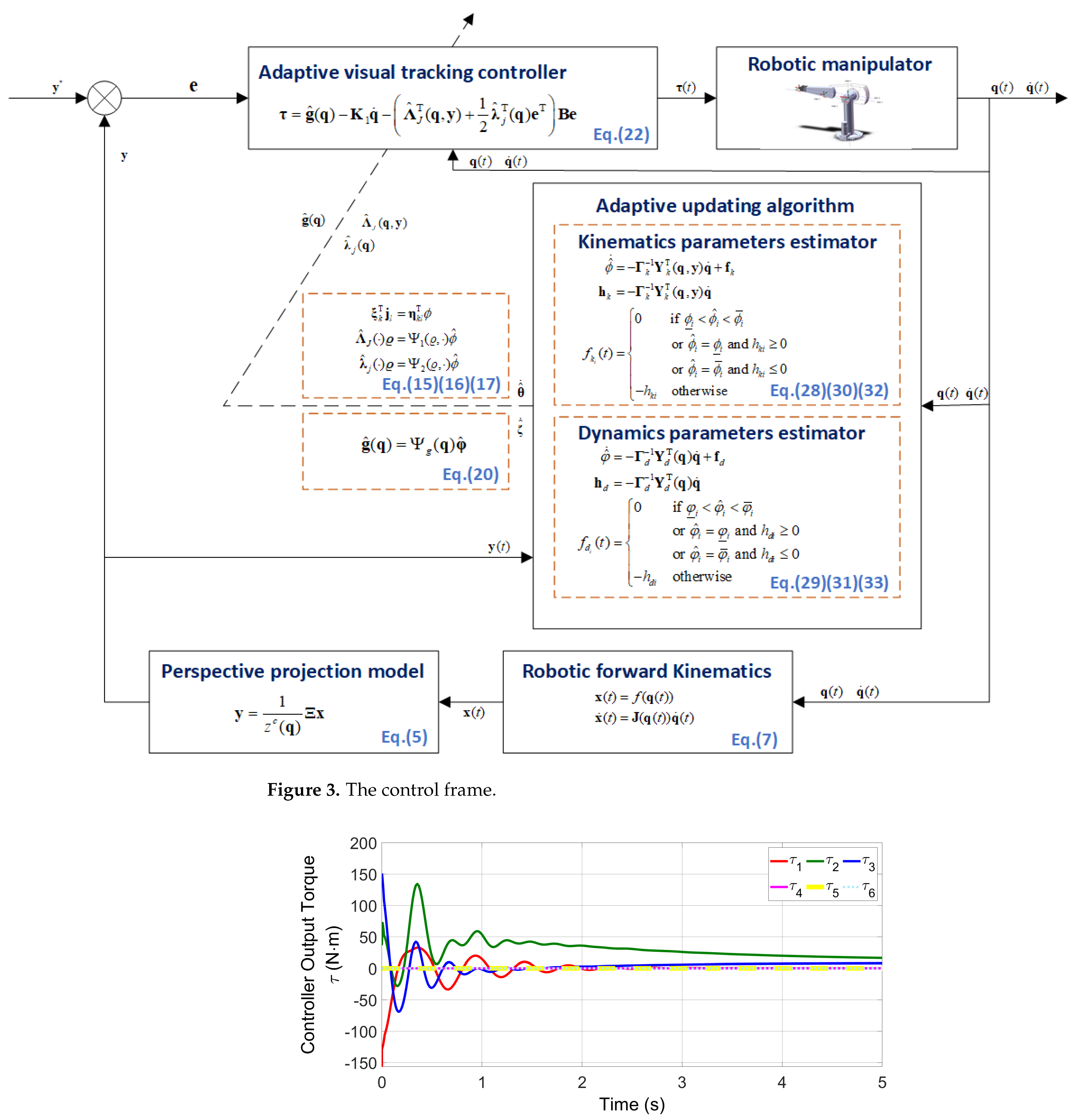
3. Uncalibrated Adaptive Visual Control Approach and Stability Analysis

To address the uncertain effects due to the lacking of precise calibration of the unknown parameters, an uncalibrated adaptive visual control approach is presented newly for the IBVS manipulator systems. Motivated by the study in [22,24,26], the design idea of our control approach has the following novelties: first, let visual and robotic physical parameters be arranged in a uniform linear form, which ensures these parameters in the closed-loop dynamics can be estimated by one adaptive law, reducing the number of adaptive algorithms; second, a new adaptive algorithm is raised, where estimated parameters are updated in an appropriate tiny range of their actual values so that the potential singularity of the estimated Jacobian matrix can be circumvented without any pre-selected trajectory point, and most importantly guarantees the asymptotic convergence of image errors.

3.1. Controller Design

The desired homogeneous image coordinate of the feature point marked on the robotic end-effector is denoted by y * , and the image error e is defined as follows
e = y y * .
Here the last component of e R 3 × 1 is always zero since y = [ u , v , 1 ] and y * = [ u d , v d , 1 ] , where u d and v d are constants. Applying the adaptive parameters, the raised controller can be presented as follows
τ = g ^ ( q ) K 1 q ˙ Λ ^ J T ( q , y ) + 1 2 λ ^ j T ( q ) e T B e ,
where B R 3 × 3 is a position positive-definite gain matrix and the related term (the last term of the right side in (22)) implies the image error feedback. Here K 1 q ˙ represents the joint velocity feedback, where K 1 R n × n is a velocity positive-definite gain matrix. Although three estimators are introduced in the controller above (22), i.e., g ^ (18), Λ ^ J T (11) and λ ^ j T (13), the last two estimators do not need to be updated, respectively. It is crucial to accomplish the parametrization of the unknown parameters before designing the adaptive laws.
Firstly, the closed-loop dynamics follows from (22) and (18) that:
M ( q ) q ¨ + 1 2 M ˙ ( q ) + C ( q , q ˙ ) q ˙ =     Λ ^ J T ( y , q ) + 1 2 λ ^ j T ( q ) e T B e K 1 q ˙ + g ˜ ( q ) ,
where g ˜ ( q ) = g ^ ( q ) g ( q ) denotes the estimated error of the gravitational force. It then follows from Proposition 3 that:
g ˜ ( q ) = Υ d ( q ) φ ˜ ,
where φ ˜ = φ ^ φ represents the estimated error of robotic physical parameters.
Subsequently, according to Proposition 2, it follows
Λ ˜ J ( q , y ) + 1 2 e λ ˜ j ( q ) T B e = Υ k ( q , y ) ϕ ˜ ,
where · ˜ denotes the estimated error of · .
Remark 6. 
The intention of developing an uncalibrated visual servoing control approach is to alleviate the impact of lacking precise measurements on the bias of the results, which by no means desires to complete the task without any prior knowledge. Thus, the selection of the initial values of unknown parameters is crucial for the convergence of task errors before implementing adaptive estimation. A too-large initial bias may cause the deterioration of control performance and even the system collapse. Compared to traditional methods, one of the advantages of the presented method is that highly servoing performance can be guaranteed even in the absence of accurate measurement.

3.2. Parameter Estimation

An adaptive algorithm is presented to update the above parameters in (24) and (25), which newly combines the Slotine-Li algorithm [30] with the parameter projection algorithm [31].
Compared with the precise calibration of ϕ and φ , the prior knowledge regarding a certain range R n where they are situated is easier to obtain, which means that an appropriate range can be found to restrict the parametric estimation in a practical case. It follows that the convex compact sets Ω k and Ω d where the unknown parameters are bounded, i.e.,
Ω k = ϕ ^ i ( 0 ) ϕ ^ ( 0 ) | ϕ ̲ i < ϕ ^ i ( 0 ) < ϕ ¯ i ,
Ω d = φ ^ i ( 0 ) φ ^ ( 0 ) | φ ̲ i < φ ^ i ( 0 ) < φ ¯ i ,
where ( · ) ̲ and ( · ) ¯ are the lower and upper bounds of the counterpart, respectively. It is desirable for the estimated parameters to always situate in these sets, which means φ ^ ( t ) Ω d and ϕ ^ ( t ) Ω k when t 0 . To this end, the parameter vectors, ϕ ^ and φ ^ , are updated by the following adaptive update laws
ϕ ^ ˙ = Γ k 1 Υ k T ( q , y ) q ˙ + f k ,
φ ^ ˙ = Γ d 1 Υ d T ( q ) q ˙ + f d ,
where Γ ( · ) is a positive-definite and diagonal matrix and f ( · ) is a correction vector, whose component f ( · ) i is constructed in the following form:
f k i = 0 if ϕ ̲ i < ϕ ^ i < ϕ ¯ i or ϕ ^ i = ϕ ̲ i and h k i 0 or ϕ ^ i = ϕ ¯ i and h k i 0 h k i otherwise ,
f d i = 0 if φ ̲ i < φ ^ i < φ ¯ i or φ ^ i = φ ̲ i and h d i 0 or φ ^ i = φ ¯ i and h d i 0 , h d i otherwise ,
where h ( · ) i is the components of h ( · ) , which is defined as follows
h k = Γ k 1 Υ k T ( q , y ) q ˙ ,
h d = Γ d 1 Υ d T ( q ) q ˙ .
Remark 7. 
The difficult convergence of estimated parameters is a well-known and challenging issue in adaptive control. Since that issue is generally harmless to the control objective, it can be ignored in the controller design. However, the Jacobian matrix estimated by an adaptive algorithm has a risk of the singular in the uncalibrated visual servo tasks due to the above difficulty, which may degrade the degree of freedom of robotic manipulators and eventually lead to the collapse of systems. Considering that the Jacobian matrix derived from the actual parameters is generally non-singular, it is reasonable to assume that the estimation in a range around its real value can also meet the non-singular requirement of the Jacobian matrix. To this end, we design a novel estimation algorithm synthesized by the technique of parameter projection in (28), which ensures the update of estimated parameters in an appropriate region and thus avoids the potential singularity of the estimated Jacobian matrix.

3.3. Stability Analysis
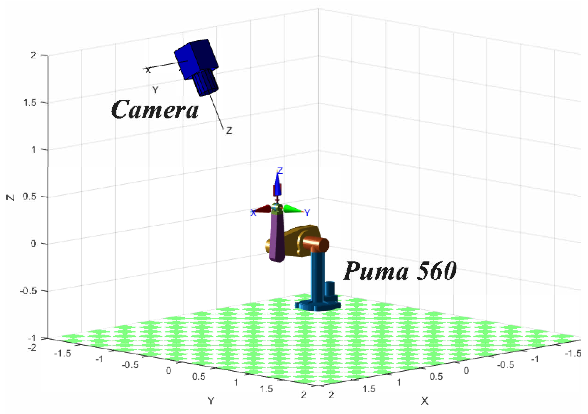
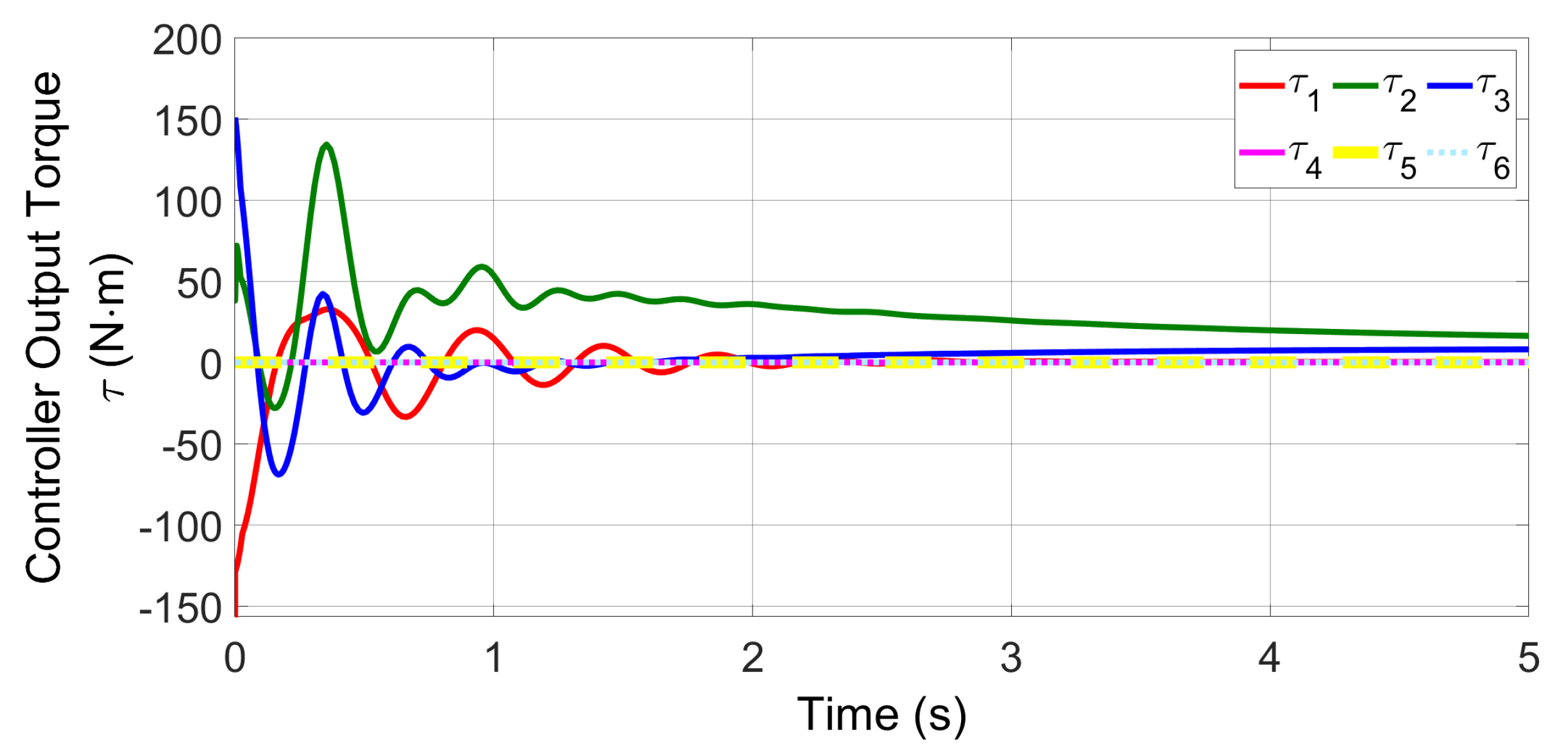
With the raised control approach, the stability analysis of the uncalibrated visual servoing system is given.
Theorem 1. 
With the unknown parameters in the controller (22) adjusted by adaptive algorithm (28)–(33), the steady-state tracking performance, i.e., lim t e ( t ) = 0 can be guaranteed, in addition to the signal boundedness of the closed-loop visual servoing system.
Proof. 
Consider the Lyapunov function
V = 1 2 z c e T B e + 1 2 q ˙ T M ( q ) q ˙ + 1 2 ϕ ˜ T Γ k ϕ ˜ + 1 2 φ ˜ T Γ d φ ˜ .
Differentiating (34) in time, it follows
V ˙ = z c e ˙ T B e + 1 2 z ˙ c e T B e + ϕ ˜ T Γ k ϕ ˜ ˙ + q ˙ T [ τ g ( q ) ] + φ ˜ T Γ d φ ˜ ˙ ,
which combined with (10), (11) and (13) results that
V ˙ = q ˙ T Λ J T ( q , y ) + 1 2 e λ j ( q ) T B e + ϕ ˜ T Γ k ϕ ˜ ˙ + q ˙ T [ τ g ( q ) ] + φ ˜ T Γ d φ ˜ ˙ .
Applying the raised controller (22) into above (36) and then incorporating with (25) and (24), we have:
V ˙ = q ˙ T K 1 q ˙ + q ˙ T Υ d ( q ) φ ˜ + φ ˜ T Γ d φ ˜ ˙ + q ˙ T Υ k ( y , q ) ϕ ˜ + ϕ ˜ T Γ k ϕ ˜ ˙ ,
which follows from (28)–(33) that
V ˙ = q ˙ T K 1 q ˙ + φ ˜ T Γ d f d + ϕ ˜ T Γ k f k .
Since the definition of f ( · ) in (30) and (31), the analysis of (38) can be divided in the following two cases: first, when the estimated parameter is within the prescribed range Ω ( · ) or tends to enter that range, f ( · ) i = 0 , which implies φ ˜ i T Γ d i i f d i = 0 and ϕ ˜ i T Γ k i i f k i = 0 ; second, when the estimated parameter is at the boundary of the prescribed range Ω ( · ) and tends to leave that range, f ( · ) i = h ( · ) i , which means φ ˜ i T Γ d i i f d i = φ ˜ i T Γ d i i h d i 0 and ϕ ˜ i T Γ k i i f k i = ϕ ˜ i T Γ k i i h k i 0 , where φ ˜ i T h d i 0 and ϕ ˜ i T h k i 0 . Thus, it follows that
φ ˜ T Γ d f d + ϕ ˜ T Γ k f k 0 ,
which implies that V ˙ is negative semi-definite, i.e.,
V ˙ q ˙ T K 1 q ˙ 0 .
The V ˙ 0 accompanied by V 0 conveys the stability of the visual servoing system and the boundedness of V, which in turn means that the variables, i.e., φ ˜ , e , ϕ ˜ , and q ˙ in (34), are bounded. It follows from (28)–(33) that ϕ ^ ˙ and φ ^ ˙ are bounded, which, incorporated with (23), implies that q ¨ is bounded. Furthermore, the boundedness of q ˙ and q ¨ conveys information about the uniform continuity of q ˙ , which follows from Barbalat’s lemma that
lim t q ˙ ( t ) = 0 .
The visual servoing system tends to an equilibrium point as q ˙ 0 , where (23) can be rewritten as follows
Λ ^ J T ( q , y ) + 1 2 λ ^ j T ( q ) e T D ( ϕ ^ , y ) B e = 0 .
To demonstrate e 0 , an auxiliary matrix D T D is constructed as follows
D T D = Θ 0 2 × 1 0 1 × 2 0 ,
from which it can be derived that R a n k ( D T D ) = R a n k ( D ) . Since Θ is nonsingular, incorporated with R a n k ( D T D ) = 2 , it follows that the image tracking error e converges to zero asymptotically as time goes to infinity. In fact, the conditions of the singularity of Θ are rigorous and even impossible for practical engineering, i.e.,
D 11 × D 22 D 12 × D 21 = 0 , D 11 × D 23 D 13 × D 21 = 0 , D 12 × D 23 D 13 × D 22 = 0 ,
which must be held simultaneously. Additionally, the estimated parameters are limited in an appropriate range around their practical value under the raised adaptive algorithm, which implies Θ can be viewed as invertible, and thus, in conclusion, e 0 . □

4. Simulation

As shown in Figure 2, an 6 DOFs industrial manipulator, Puma 560, is utilized to give a simulation verification of the proposed method. Conventionally, the description of the orientations and the poses of serial links are introduced to the Denavit-Hartenberg parameters represent method (D−H) which indicates the physical features of the manipulator with four parameters. The D−H represents the parameters of the manipulator as shown in Table 1. The ith non-zero link offset and link length are represented by d i and a i , respectively. Meanwhile, the mass of the serial links is listed as follows, m 1 = 0 , m 2 = 17.4 and m 3 = 4.8 , m 4 = 0.82 , m 5 = 0.34 and m 6 = 0.09 . Since the computing complexity of the proposed scheme is determined by the number of unknown parameters, only the uncertainties caused by the non-zero parameters are taken into account.
The position/orientation of the camera are unrestricted if the FOV constraint is satisfied, the parameters of which are given by
Ξ = 750 256 443.4 1186.5 0 393.5 818.4 743.6 0 0.5 0.9 2.4 .
The parameter vector ϕ = ξ 3 T ξ 2 T ξ 1 T d 4 d 3 a 3 a 2 , where ⊗ is a Kronecker product operator, and the actual value of which is shown as follows, [−0.374, −0.130, −0.018, −0.374, 0.216, 0.075, 0.01, 0.216, 0, 0, 0, 0, −353.387, −122.802, −16.614, −353.387, −169.922, −59.048, −7.988, −169.922, 0, 0, 0, 0, −191.462, −66.533, −9.001, −191.462, 110.541, 38.413, 5.197, 110.542, 323.850, 112.538, 15.225, 323.85]. Additionally, the parameter vector φ is given by [0.09, 0.82, 4.8, 17.4, 0.039, 0.147, 0.354, 0.002, 0.007, 0.017, 0.097, 0.039, 0.147, 0.354, 2.073, 7.513]. For operationalizing the adaptive law, let ϕ ¯ = 1.5 ϕ , ϕ ̲ = 0.75 ϕ , ϕ ^ ( 0 ) = 0.85 ϕ , and so does φ . The control frame in matlab simulink is shown in Figure 3, where the controller input, namely desired image coordinate, is set as y * = [ 600 , 300 ] T .
Observing the torque in Figure 4, the τ is bounded and convergent. Furthermore, the angles q of the robotic joint, shown in Figure 5, have a convergent performance as well. As we can see the convergence to zero of the angular velocity q ˙ of the robotic joint in Figure 6 demonstrates the validity of the deduction in (41). This declares that there is indeed an equilibrium point in our control system, in other words, the visual seroving system incorporated proposed control scheme is stable.
Since the precise measurement of the model parameters of the robotic manipulator and the visual camera is almost inaccessible in practical implementation, the uncertainties caused by those parameters in kinematics and dynamics will be the key factor of the accuracy of the control target. However, the following results will show us the effectiveness of the proposed adaptive algorithm which utilize the approximate model parameter to estimate the unknown torques and even to help the controller to achieve the control target. The estimation of the ϕ and φ can be seen in Figure 7 and Figure 8, respectively. It is more exciting to see in Figure 9 that the estimated gravitational torque in the controller has a good performance in following its actual gravitational torque, which can direct improve the accuracy of the image tracking.
The 3−D space trajectory of the point marked on the end-effector of the robotic manipulator is depicted in Figure 10, correspondingly its plane trajectory on the image plane is illustrated in Figure 11. Observing the trajectory in Figure 10 and Figure 11, we can find that the feature point is successfully converged to the desired point on image space.
Note that the symbol □ in Figure 10 represents the final position of the end-effector, not the desired one in task space, which means that the end-effector is not necessarily driven to the desired location in task space while the image tracking error converges to zero. Although some existing studies [22,23,24,25] propose a method to regulate the spacial position of the end-effector by a sufficient pre-selected point on a 3−D trajectory, it is an impractical task for an uncalibrated visual servoing control. The consistent convergence of image and spatial position is a challenging problem for the uncalibrated IBVS control scheme with monocular vision.
Furthermore, the image tracking error converges asymptotically toward zero, as shown in Figure 12, which demonstrates the conclusion in Theorem 1 that the adaptive controller can ensure the steady-state tracking performance of the visual servoing system even in presence of uncertainties in kinematics and dynamics.
Remark 8. 
Despite the desired control performance that can be achieved for a simulated 6−DOFs manipulator, the raised theoretical control scheme can have some restrictions in real applications. From the simulation study, we find that the number of adaptive laws will increase significantly with the degrees of freedom, so a computational burden may be caused in the applications involving rather high degrees of freedom, which can have destroying effects on closed-loop system performance. Besides, the proposed setpoint control scheme may be insufficient to meet the performance requirements of real applications due to the absence of constraints on the posture and trajectory of manipulators.
Remark 9. 
When implementing the proposed control scheme on practical manipulators, some additional issues could be encountered, e.g.,
  • Nonlinear dynamics. Although the dynamics of manipulators have been considered in the proposed method, there are still some unmodeled dynamic factors ignored, such as the Coulomb friction, the viscous friction, and the motor dynamics, which may deteriorate system performance and even lead to system collapse in a practical scenario.
  • Nonlinear constraint of actuators. The nonlinear constraints widely exist in many physical actuators, which may lead to errors in the practical results and even instability of the system. To address it, the nonlinear constraints of actuators, such as the backlash, dead zone, saturation, and hysteresis, should be compensated in practical applications. Furthermore, the unknown actuator failures should also be considered regarding real-world visual servo tasks, which would lead to catastrophic results once a failure occurs.
  • Noise and disturbances. The image-based visual servoing control method is sensitive to noise and disturbances in the image measurements, which can affect the accuracy and stability of the control system. In our research, the image noise and corresponding image processing techniques do not account for this, but they should be considered in practical applications. Additionally, the variations in lighting, occlusions, and other environmental factors should be considered too, which may significantly impact the quality of visual feedback.
  • Real-time performance. Visual servoing systems may suffer from latency issues, which may be caused by communication and sampling, thus achieving the real-time performance of manipulators remains a challenge for real-world scenarios.
These issues mentioned above may be regarded as our next study in the future.

5. Conclusions

In our study, an uncalibrated adaptive visual servoing control scheme is proposed novelly. The kinematic and dynamic uncertainties caused by unknown parameters (including extrinsic/intrinsic parameters of a camera and physical parameters of a robotic manipulator) are addressed in this paper. Specifically, a depth-independent composite Jacobian matrix is used to parametrize the visual parameters combined with the robotic parameters in a linear form. The proposed adaptive algorithm is applied to update the estimated parameters in order to guarantee that the image tracking error asymptotically converges to zero. At present, however, our raised control scheme is only studied in theory, and the illustration of its effectiveness is mainly by means of the stability analysis with rigorous proof, and the simulation technique. To verify the proposed control scheme experimentally, there are still some issues, as mentioned in Remark 9, to be addressed, which may be regarded as our next study in the future.

Author Contributions

Conceptualization, G.L.; methodology, W.Y.; software, A.L.; validation, G.L. and Y.C.; formal analysis, Y.C.; writing—original draft preparation, W.Y.; writing—review and editing, A.L.; Investigation, L.Z.; Visualization, L.Z. All authors have read and agreed to the published version of the manuscript.

Funding

This research was funded in part by the Tertiary Education Scientific research project of Guangzhou Municipal Education Bureau under Grant [No. 202235364], in part by the Science and Technology Program of Guangzhou, China under Grant [No. 201804010098], in part by the Special projects in key fields of colleges and universities in Guangdong Province under Grant [No. 2021ZDZX1109, No. 2022ZDZX1070], in part by the Basic and Applied Basic Research Foundation of Guangzhou under Grant 2023A04J0345, and in part by the Basic and Applied Basic Research Foundation of Guangdong Province under Grant 2019A1515012109.

Institutional Review Board Statement

Not applicable.

Informed Consent Statement

Not applicable.

Data Availability Statement

Not applicable.

Conflicts of Interest

The authors declare no conflict of interest.

References

  1. Shirai, Y.; Inoue, H. Guiding a robot by visual feedback in assembling tasks. Pattern Recognit. 1973, 5, 99–108. [Google Scholar] [CrossRef]
  2. Jing, C.; Xu, H.; Niu, X. Adaptive sliding mode disturbance rejection control with prescribed performance for robotic manipulators. ISA Trans. 2019, 91, 41–51. [Google Scholar] [CrossRef] [PubMed]
  3. Moreno-Valenzuela, J.; González-Hernández, L. Operational space trajectory tracking control of robot manipulators endowed with a primary controller of synthetic joint velocity. ISA Trans. 2011, 50, 131–140. [Google Scholar] [CrossRef] [PubMed]
  4. Hill, J. Real time control of a robot with a mobile camera. In Proceedings of the International Symposium on Industrial Robots; Society of Manufacturing Engineers: Dearborn, MI, USA, 1979; pp. 233–246. [Google Scholar]
  5. Hutchinson, S.; Hager, G.; Corke, P. A tutorial on visual servo control. IEEE Trans. Robot. Autom. 1996, 12, 651–670. [Google Scholar] [CrossRef] [Green Version]
  6. Staniak, M.; Zieliński, C. Structures of visual servos. Robot. Auton. Syst. 2010, 58, 940–954. [Google Scholar] [CrossRef]
  7. Tan, M.; Liu, Z.; Chen, C.P.; Zhang, Y. Neuroadaptive asymptotic consensus tracking control for a class of uncertain nonlinear multiagent systems with sensor faults. Inf. Sci. 2022, 584, 685–700. [Google Scholar] [CrossRef]
  8. Tan, M.; Liu, Z.; Chen, C.P.; Zhang, Y.; Wu, Z. Optimized adaptive consensus tracking control for uncertain nonlinear multiagent systems using a new event-triggered communication mechanism. Inf. Sci. 2022, 605, 301–316. [Google Scholar] [CrossRef]
  9. Hu, G.; MacKunis, W.; Gans, N.; Dixon, W.E.; Chen, J.; Behal, A.; Dawson, D. Homography-Based Visual Servo Control With Imperfect Camera Calibration. IEEE Trans. Autom. Control 2009, 54, 1318–1324. [Google Scholar] [CrossRef] [Green Version]
  10. Wang, K.; Liu, Y.; Li, L. Vision-based tracking control of nonholonomic mobile robots without position measurement. In Proceedings of the 2013 IEEE International Conference on Robotics and Automation, Karlsruhe, Germany, 6–10 May 2013; pp. 5265–5270. [Google Scholar]
  11. Lippiello, V.; Siciliano, B.; Villani, L. Position-Based Visual Servoing in Industrial Multirobot Cells Using a Hybrid Camera Configuration. IEEE Trans. Robot. 2007, 23, 73–86. [Google Scholar] [CrossRef]
  12. Chaumette, F.; Hutchinson, S. Visual servo control. I. Basic approaches. IEEE Robot. Autom. Mag. 2006, 13, 82–90. [Google Scholar] [CrossRef]
  13. Hwang, M.; Chen, Y.J.; Ju, M.Y.; Jiang, W.C. A fuzzy CMAC learning approach to image based visual servoing system. Inf. Sci. 2021, 576, 187–203. [Google Scholar] [CrossRef]
  14. Qian, J.; Su, J. Online estimation of image Jacobian matrix by Kalman-Bucy filter for uncalibrated stereo vision feedback. In Proceedings of the 2002 IEEE International Conference on Robotics and Automation (Cat. No. 02CH37292), Washington, DC, USA, 11–15 May 2002; Volume 1, pp. 562–567. [Google Scholar]
  15. Hosoda, K.; Asada, M. Versatile visual servoing without knowledge of true Jacobian. In Proceedings of the IEEE/RSJ International Conference on Intelligent Robots and Systems (IROS’94), Munich, Germany, 12–16 September 1994; Volume 1, pp. 186–193. [Google Scholar]
  16. Piepmeier, J.; McMurray, G.; Lipkin, H. Uncalibrated dynamic visual servoing. IEEE Trans. Robot. Autom. 2004, 20, 143–147. [Google Scholar] [CrossRef]
  17. Armstrong Piepmeier, J.; Gumpert, B.; Lipkin, H. Uncalibrated eye-in-hand visual servoing. In Proceedings of the 2002 IEEE International Conference on Robotics and Automation (Cat. No. 02CH37292), Washington, DC, USA, 11–15 May 2002; Volume 1, pp. 568–573. [Google Scholar]
  18. Wang, F.; Liu, Z.; Chen, C.; Zhang, Y. Adaptive neural network-based visual servoing control for manipulator with unknown output nonlinearities. Inf. Sci. 2018, 451-452, 16–33. [Google Scholar] [CrossRef]
  19. Cheah, C.; Hirano, M.; Kawamura, S.; Arimoto, S. Approximate Jacobian control for robots with uncertain kinematics and dynamics. IEEE Trans. Robot. Autom. 2003, 19, 692–702. [Google Scholar] [CrossRef]
  20. Cai, C.; Dean-León, E.; Mendoza, D.; Somani, N.; Knoll, A. Uncalibrated 3D stereo image-based dynamic visual servoing for robot manipulators. In Proceedings of the 2013 IEEE/RSJ International Conference on Intelligent Robots and Systems, Tokyo, Japan, 3–7 November 2013; pp. 63–70. [Google Scholar]
  21. Cheah, C.C.; Liu, C.; Slotine, J.J.E. Adaptive Vision based Tracking Control of Robots with Uncertainty in Depth Information. In Proceedings of the 2007 IEEE International Conference on Robotics and Automation, Roma, Italy, 10–14 April 2007; pp. 2817–2822. [Google Scholar]
  22. Liu, Y.H.; Wang, H.; Wang, C.; Lam, K.K. Uncalibrated visual servoing of robots using a depth-independent interaction matrix. IEEE Trans. Robot. 2006, 22, 804–817. [Google Scholar]
  23. Wang, H.; Liu, Y.H.; Zhou, D. Dynamic Visual Tracking for Manipulators Using an Uncalibrated Fixed Camera. IEEE Trans. Robot. 2007, 23, 610–617. [Google Scholar] [CrossRef]
  24. Wang, H.; Jiang, M.; Chen, W.; Liu, Y.H. Visual servoing of robots with uncalibrated robot and camera parameters. Mechatronics 2012, 22, 661–668. [Google Scholar] [CrossRef]
  25. Liu, Y.H.; Wang, H.; Chen, W.; Zhou, D. Adaptive visual servoing using common image features with unknown geometric parameters. Automatica 2013, 49, 2453–2460. [Google Scholar] [CrossRef]
  26. Cheah, C.C.; Liu, C.; Slotine, J.J.E. Adaptive Jacobian vision based control for robots with uncertain depth information. Automatica 2010, 46, 1228–1233. [Google Scholar] [CrossRef]
  27. Wang, F.; Liu, Z.; Chen, C.P.; Zhang, Y. Robust adaptive visual tracking control for uncertain robotic systems with unknown dead-zone inputs. J. Frankl. Inst. 2019, 356, 6255–6279. [Google Scholar] [CrossRef]
  28. Guo, D.; Sun, F.; Fang, B.; Yang, C.; Xi, N. Robotic grasping using visual and tactile sensing. Inf. Sci. 2017, 417, 274–286. [Google Scholar] [CrossRef]
  29. Liu, A.; Lai, G.; Liu, W. Adaptive Visual Control of Robotic Manipulator With Uncertainties in Kinematics and Dynamics. In Proceedings of the 2021 China Automation Congress (CAC), Beijing, China, 22–24 October 2021; pp. 7232–7237. [Google Scholar]
  30. Slotine, J.J.; Li, W. On the Adaptive Control of Robot Manipulators. Int. J. Robot. Res. 1987, 6, 49–59. [Google Scholar] [CrossRef]
  31. Krstic, M.; Kokotovic, P.V.; Kanellakopoulos, I. Nonlinear and Adaptive Control Design; John Wiley & Sons, Inc.: Hoboken, NJ, USA, 1995. [Google Scholar]
  32. Alavandar, S.; Nigam, M. New hybrid adaptive neuro-fuzzy algorithms for manipulator control with uncertainties—Comparative study. ISA Trans. 2009, 48, 497–502. [Google Scholar] [CrossRef] [PubMed]
  33. Huang, C.; Xie, L.; Liu, Y. PD plus error-dependent integral nonlinear controllers for robot manipulators with an uncertain Jacobian matrix. ISA Trans. 2012, 51, 792–800. [Google Scholar] [CrossRef]
Figure 1. Configuration of the visual feedback system.
Actuators 12 00143 g001
Figure 2. The visual servoing system in RTB.
Actuators 12 00143 g002
Figure 3. The control frame.
Actuators 12 00143 g003
Figure 4. The controller output joint torque.
Actuators 12 00143 g004
Figure 5. The robotic joint angle.
Actuators 12 00143 g005
Figure 6. The robotic joint velocity.
Actuators 12 00143 g006
Figure 7. Some components of the adaptive vector ϕ ^ .
Actuators 12 00143 g007
Figure 8. The adaptive vector φ ^ .
Actuators 12 00143 g008
Figure 9. The compensation of the gravity.
Actuators 12 00143 g009
Figure 10. 3−D trajectory of the marked point.
Actuators 12 00143 g010
Figure 11. 2−D trajectory of the projection of the feature point.
Actuators 12 00143 g011
Figure 12. The image tracking error versus time.
Actuators 12 00143 g012
Table 1. D−H Represent Parameters.
JointAngle (Rad)Offset (m)Length (m)Twist (Rad)
1 q 1 00 1 2 π
2 q 2 00.43180
3 q 3 0.150050.0203 1 2 π
4 q 3 0.43180 1 2 π
5 q 3 00 1 2 π
6 q 3 000
Disclaimer/Publisher’s Note: The statements, opinions and data contained in all publications are solely those of the individual author(s) and contributor(s) and not of MDPI and/or the editor(s). MDPI and/or the editor(s) disclaim responsibility for any injury to people or property resulting from any ideas, methods, instructions or products referred to in the content.

