Article

Distributed Model Predictive Control with Particle Swarm Optimizer for Collision-Free Trajectory Tracking of MWMR Formation

1
Faculty of Information Technology, Beijing University of Technology, Beijing 100124, China
2
Engineering Research Center of Digital Community, Ministry of Education, Beijing 100124, China
*
Author to whom correspondence should be addressed.
Actuators 2023, 12(3), 127; https://doi.org/10.3390/act12030127
Submission received: 7 February 2023 / Revised: 8 March 2023 / Accepted: 14 March 2023 / Published: 16 March 2023
(This article belongs to the Section Control Systems)

Abstract

:
The distributed model predictive control (DMPC) strategy with particle swarm optimization (PSO) is applied to solve the collision-free trajectory tracking problem for the mecanum-wheeled mobile robot (MWMR) formation. Under the leader–follower framework, the predictive model is established considering the kinematics and dynamics of the MWMR with the uncertainties and external disturbances. Based on the information from itself and its neighbors, each MWMR is assigned its own finite-horizon optimal control problem, of which the objective/cost function consists of formation maintenance, trajectory tracking, and collision avoidance terms, and the control inputs of each MWMR are computed synchronously in a distributed manner. PSO serves as the fast and effective optimizer to find feasible solutions to these finite-horizon optimal control problems. Further, the feedback emendation is implemented using a double closed-loop compensator to efficiently inhibit the influence of unknown dynamics in real time. The stability of the proposed distributed formation control approach is strictly analyzed. Numerical simulations confirmed the robustness and effectiveness of the control approach in obstacle environments.

1. Introduction

In recent years, extensive research has focused on the motion control of mobile robots [1,2,3,4]. As a typical omnidirectional mobile robot, the mecanum-wheeled mobile robot (MWMR) has been widely used in family service and industrial production fields because of its flexibility in confined spaces and capability of moving to any direction without a turning radius [
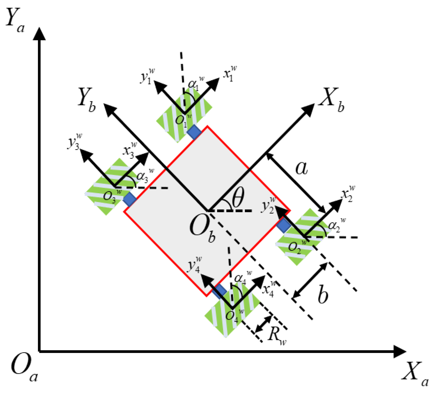
5]. Four specially made mecanum wheels are symmetrically mounted around the mobile robot, while each mecanum wheel is separately driven by a motor. Some rollers are angled at 45° to the hub circumference of a mecanum wheel [6], which enables the MWMR to move in sideways.
Mobile robot formation aims to control multiple mobile robots to synchronously move in a certain formation pattern, which is one of the hotspot problems in the study of robotics [7,8]. There are some typical techniques for solving the formation control problem, for example, the leader–follower method, virtual structure method, and behavior-based methods [9,10,11,12,13]. Formation control of multiple MWMRs has also attracted extensive attention from researchers. Aditya et al. [14] established the collaborative kinematics of the MWMR’s system to realize the cooperative transformation of large-scale goods in formation. Mehrez et al. [15] established a formation set-point stabilization of MWMRs using the model predictive control (MPC) method without terminal constraints. However, the MWMR actually is a complex mechanic system with kinematics, dynamics, and input saturation constraints. Treating it as a mass point or only considering the kinematics will reduce the control accuracy.
The MWMR has the complexity of nonlinearity, uncertainty, and external disturbances in its dynamics. Additionally, the input saturation constraints can also bring great challenge to the precise control of MWMRs [16,17]. Alakshendra et al. [18] derived a generalized dynamic equation of a MWMR using Newton–Euler method. Sun et al. [19] presented the integrated kinematic–dynamic model of MWMRs, and the formation control of MWMRs under changing topologies was considered [20,21]. However, uncertainties and unmodeled disturbances can usually bring up the instability in the control system [22,23]. Thus, it is highly necessary to handle the uncertainties and disturbances in the MWMRs’ formation control problem. Lu et al. [22] employed the artificial neural network to estimate various uncertain disturbances and proposed a novel adaptive sliding mode control (SMC) method to design the trajectory tracking controller of MWMR. Zhao et al. [23] employed a fuzzy approximator to approximate unknown dynamics and applied the fixed-time extended state observer (FTESO) to estimate external disturbances for improving the tracking accuracy of MWMR. Wang et al. [
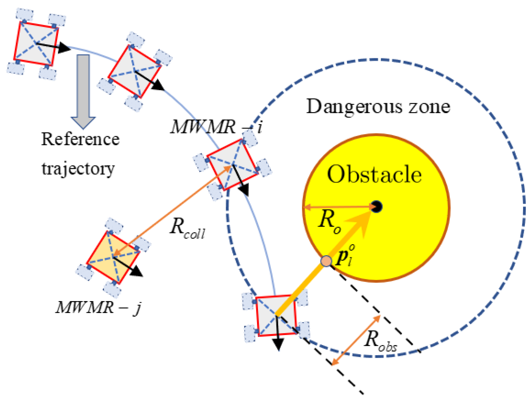
24] proposed a robust control strategy combing the adaptive SMC method and extended state observer (ESO) to compensate for total disturbances during the formation control process of MWMRs. However, the observer-based method can only estimate the constant and slowly varying parameters. In real contexts, uncertainties and disturbances are usually time-varying parameters, which are more suitable for feedback compensation strategies. Moreover, the collision of MWMRs with obstacles and other MWMRs should be avoided to ensure the safety of the MWMRs’ formation [25]. Potential field-based methods are often used to handle the collision avoidance [26,27], but these methods have the drawback of trapping in the local extremum. Barrier function-based finite-time SMC is also an effective control method for mobile robots under uncertainties and input saturations [28,29]. Mostafa et al. [28] proposed an optimal adaptive barrier function-based super-twisting SMC scheme for the trajectory tracking control of parallel robots with highly complex dynamics in the presence of uncertainties and external disturbances, where the global property of the controller eliminates the reaching phase, thereby guaranteeing system stability, and the barrier function-based adaptation law removes the requirement to know the upper bounds of the external disturbances. Khalid et al. [29] proposed an adaptive barrier function-based non-singular terminal SMC approach for the trajectory tracking of a quadrotor drone, where the non-singular terminal sliding surface was employed to ensure the finite time convergence of the linear sliding surfaces and tracking errors.
Distributed model predictive control (DMPC) is an effective method to handle the distributed cooperative control problem with dynamic uncertainties and disturbances [30,31], and can be applied to formation control of mobile robots [32,33,34,35]. Using the distributed framework, robots can share information with neighbors and solve their own local optimal control commands based on the prediction model. Zhao et al. [32] proposed a DMPC framework for autonomous underwater vehicles (AUV) through combining the alternating direction multiplier (ADMM) solver with feedforward compensation to deal with certain disturbances. Mario et al. [33] proposed a DMPC law for differentially driven robots and ensured system asymptotic stability. Qin et al. [34] proposed a Nash-based DMPC strategy for the formation control of multiple mobile robots, and the optimal control input is solved by a primal–dual neural network. However, there are few studies on MWMR formation control using the DMPC method. Wang et al. [24] applied linear MPC in the outer loop kinematic controller of MWMRs, but dynamics were not considered. Xiao et al. [35] proposed the self-triggered organized formation (STOF) system by combing the DMPC framework and the consensus protocol to achieve the smoother control performance for the MWMR’s formation, but the collision avoidance and obstacle avoidance were not considered.
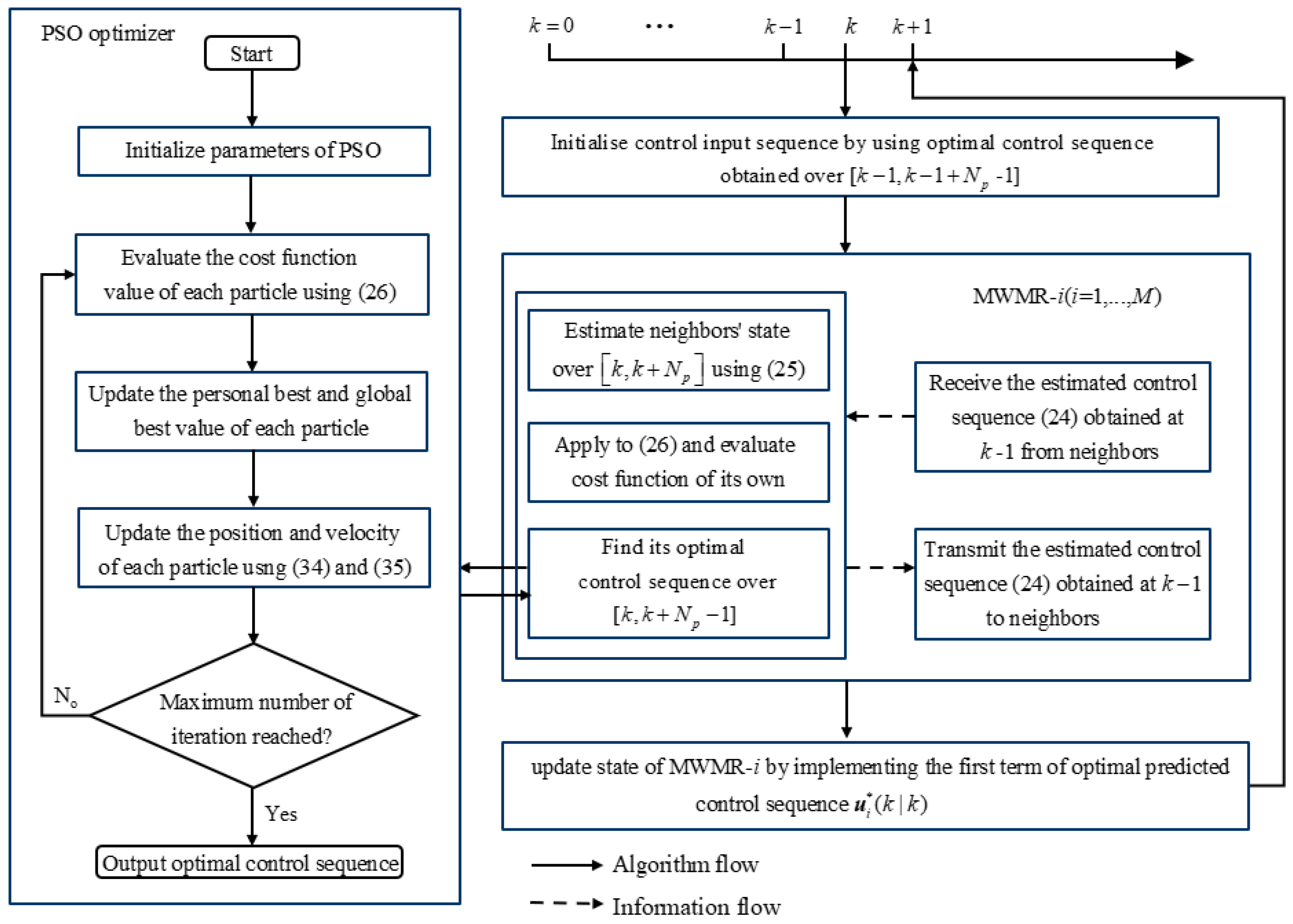
The particle swarm optimization (PSO) algorithm is a typical swarm intelligence optimization algorithm with the advantages of being a concise concept, having convenient implementation, high precision, and fast convergence. Benefitting from a fast convergence speed and global search capability, the PSO optimizer is more efficient and stable than traditional optimization solvers. Today, there are still many recent studies applying the PSO optimizer in solving MPC problems, achieving good results [36,37,38,39,40,41].
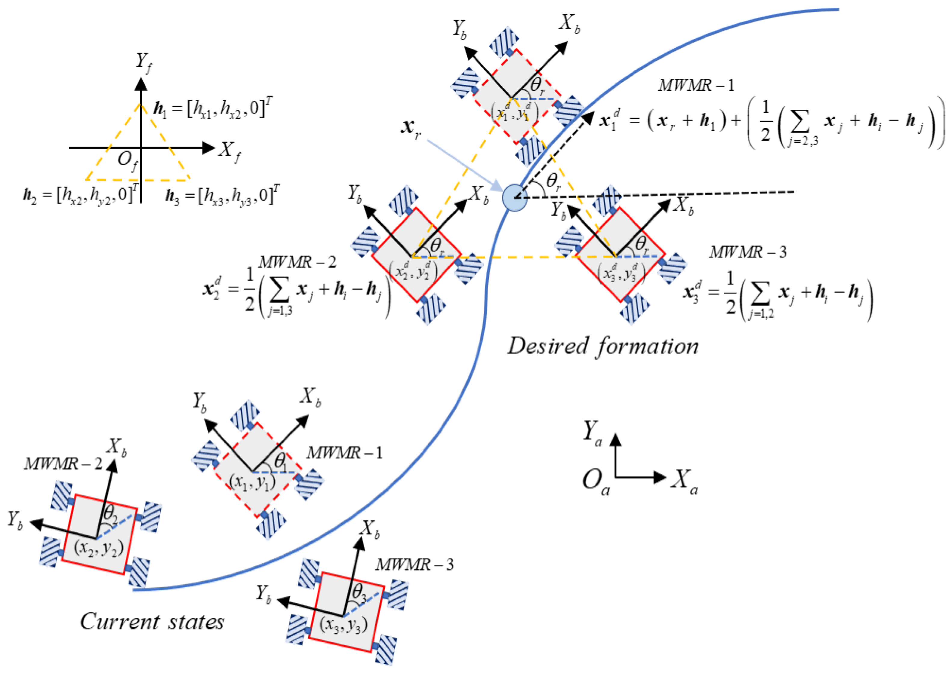
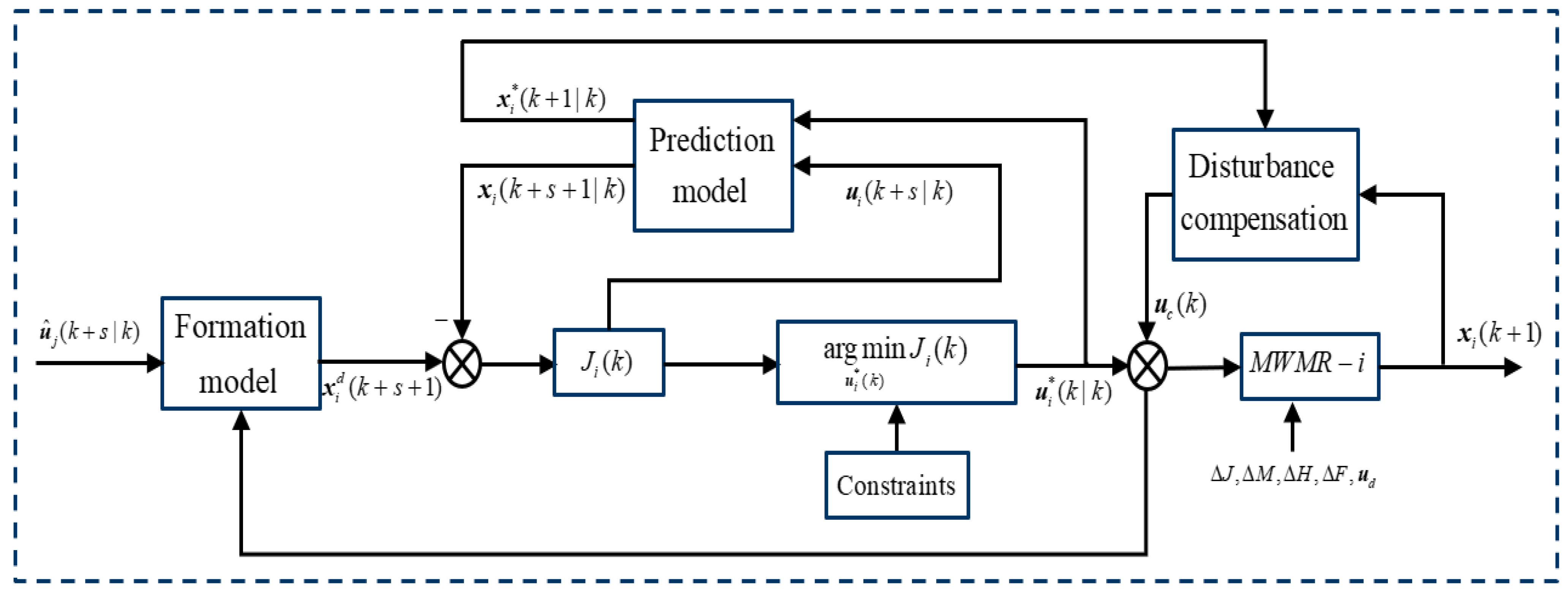
Although lots of existing works have been available, the issue of formation control of MWMRs has not been well addressed yet when simultaneously considering various physical constraints, including kinematics/dynamics constraints, uncertainties, and disturbances, as well as collision and obstacle avoidance. In this paper, taking into account the model physical constraints and uncertainties, the collision-free trajectory tracking control of the MWMR’s formation is solved using a closed-loop DMPC strategy. Based on the leader-follower framework, the formation predictive model, which describes both the kinematics and dynamics of MWMRs with the uncertainties and external disturbances, is established. Under the distributed protocol, the MWMR can share the information among itself and its neighbors. A finite-horizon optimal control problem is assigned to each MWMR to minimize the objective/cost function consisting of formation maintenance, trajectory tracking, and collision avoidance terms. The PSO algorithm is introduced to find feasible optimal control solutions for each MWMR. Then, a novel double closed-loop disturbance feedback controller is proposed to compensate for model uncertainties and external disturbances. Theoretical analysis assures the stability of the proposed distributed formation control approach. The main contribution of the paper is described in the following part:
(1)
The leader–follower predictive model of MWMR formation, considering the kinematics and dynamics with the uncertainties and external disturbances, is established.
(2)
By combining information from itself and its neighbors, each MWMR is given its own finite-horizon optimal control problem within the proposed framework of DMPC, whose objective/cost function compromises of formation maintenance, trajectory tracking, and collision avoidance terms simultaneously, is established.
(3)
A PSO-based control solver is used to find the feasible solutions to these finite-horizon optimal control problems, which shows better performance than traditional solvers.
(4)
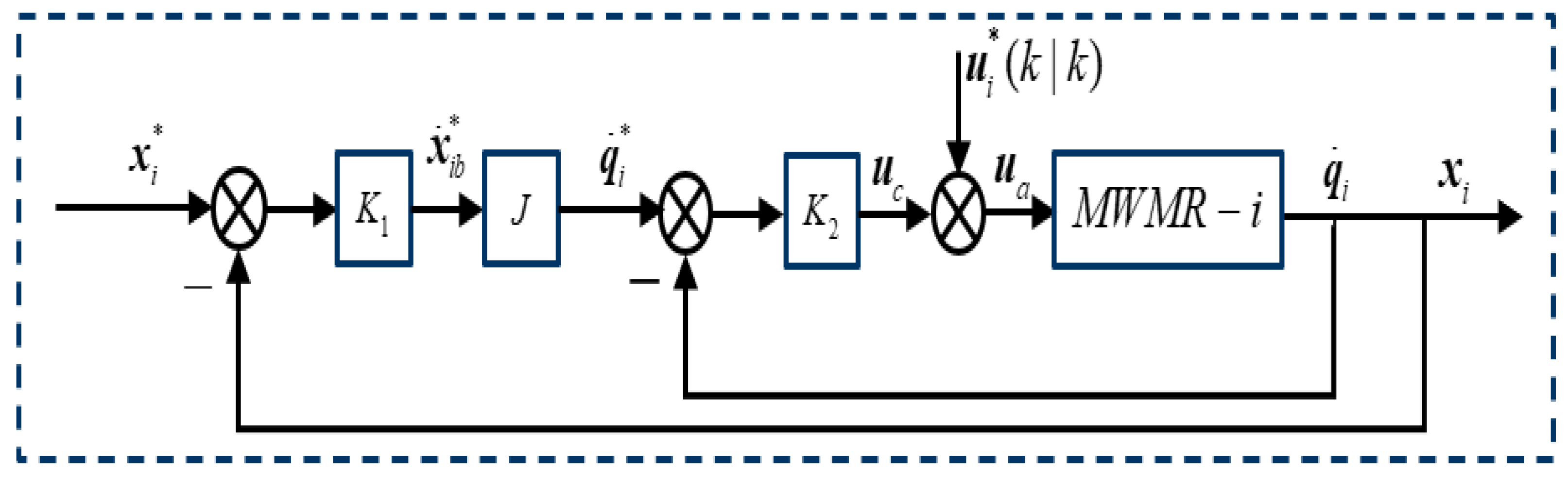
A novel double closed-loop feedback compensation controller is developed to compensate for model uncertainties and external disturbances in real-time.
The rest of this paper is constructed as follows. Section 2 describes the problem description and definition of the MWMR’s formation. Section 3 presents the proposed PSO-based DMPC controller for the MWMR’s formation in detail, including the DMPC framework, PSO optimizer, double closed-loop feedback compensator, as well as the stability analysis. In Section 4, numerical results demonstrate the superiority and effectiveness of our proposed strategy. Section 5 gives the concluding remarks finally.

2. Problem Description

2.1. MWMR Model

In this section, both the kinematic and dynamic models of MWMRs with uncertainties and time-varying external disturbances are presented. Kinematics can depict the relationship between the position and velocity of the robot, and then, dynamics further establish the relationship between the control inputs and velocity of the robot.

2.1.1. Kinematics

In order to set up the mathematics model of kinematics for the MWMR, two coordinate frame systems are constructed firstly. As is shown in Figure 1, X a O a Y a denotes the world/global frame, X b O b Y b denotes the local/body frame x = [ x , y , θ ] T , and x b = [ x b , y b , θ ] T denotes the posture vectors defined in X a O a Y a and X b O b Y b , respectively, and:
x ˙ = T ( θ ) x ˙ b
where T ( θ ) is the rotation matrix of the local frame with respect to global frame, as follows:
T ( θ ) = [ cos θ sin θ 0 sin θ cos θ 0 0 0 1 ]
i w represents the angle between axes of the i-th wheel rollers and the mecanum wheel frame x i w O i w y i w , i = 1,2,3,4, and i w = π / 4 ; Rw is the wheel radius; a and b are half the length and width of the MWMR, respectively.
As to the i-th MWMR, the inverse kinematics can be represented as:
q ˙ i = J x ˙ i b
J = 1 R w [ 1 1 ( a + b ) 1 1 a + b 1 1 ( a + b ) 1 1 a + b ]
where x i b = [ x i b , y i b , θ i b ] T is the state vector of MWMR-i in the body frame; q ˙ i = [ q ˙ i 1 , q ˙ i 2 , q ˙ i 3 , q ˙ i 4 ] T is the angular velocities of four mecanum wheels of MWMR-i.
Define J+ as the Moore–Penrose inverse of J that is shown in the following equation:
J + = ( J T J ) 1 J T
Therefore, the kinematic model of MWMR-i is:
x ˙ i b = J + q ˙ i
where J+ can be represented as:
J + = R w 4 [ 1 1 1 1 1 1 1 1 1 a + b 1 a + b 1 a + b 1 a + b ]
Combining (1) and (6), the kinematic model of MWMR-i with respect to the global frame can be expressed as follows:
x ˙ i = T ( θ i ) J + q ˙ i
where θ i represents the heading angle of MWMR-i.

2.1.2. Dynamics

The mathematics model of the MWMR dynamics is developed using the Lagrange’s equation. For the MWMR-i, the kinematic energy equation can be expressed as:
K i = 1 2 m ( x ˙ i 2 + y ˙ i 2 ) + 1 2 J z θ ˙ i 2 + 1 2 J w ( q ˙ i 1 2 + q ˙ i 2 2 + q ˙ i 3 2 + q ˙ i 4 2 )
where m is the total mass of the MWMR, J z = m ( 2 a ) 2 + ( 2 b ) 2 12 is the moment of inertia of MWMR around the zb-axis, mw is the mass of the mecanum wheel, and J w = m w R w 2 2 is the moment of inertia of wheels around the center of revolution. Further, the loss energy due to the viscous friction is:
D = 1 2 q ˙ i T H n q ˙ i
where H n = d i a g ( λ 1 , λ 2 , λ 3 , λ 4 ) denotes the coefficient of the wheel’s viscous friction.
Let the Lagrangian function be
L i = K i V i
where Vi is the potential energy of MWMR-i on the horizontal plane and equals to zero. Using the Lagrangian equation, the following equation can be yielded:
d d t q ˙ i L i q i L i = u i q ˙ i D R w 2 F ( q ˙ i ) R w
where u i = [ u i 1 , u i 2 , u i 3 , u i 4 ] T denotes the driving torque vector by the four motors of MWMR-i. The static friction F ( q ˙ i ) is denoted by F ( q ˙ i ) = [ f sgn ( q ˙ i 1 ) , f sgn ( q ˙ i 2 ) , f sgn ( q ˙ i 3 ) , f sgn ( q ˙ i 4 ) ] T . f = μ m w g represents the maximum static friction and μ is the frictional coefficient. g = 9.8 m / s 2 is the gravity acceleration.
Manipulating (12), the dynamic model of MWMR-i can be represented as:
u i = M n q ¨ i + H n q ˙ i R w 2 + F ( q ˙ i ) R w
where
M n = [ J A + J B + J w J A J A J B J A J A J A + J B + J w J B J A J A J A J B J A J A + J B + J w J A J B J A J A J A J A + J B + J w ]
where J A = J Z R w 2 16 ( a + b ) 2 , J B = m R w 2 8 . Then, substituting (8) into (13), the second-order differential equation for MWMR-i can be obtained as follows:
x ¨ i = T ( θ i ) J + M n 1 u i R w T ( θ i ) J + M n 1 F ( q ˙ i ) [ T ( θ i ) T ˙ 1 ( θ i ) + R w 2 T ( θ i ) J + M n 1 H n J T 1 ( θ i ) ] x ˙ i

2.1.3. Model under Uncertainties and Disturbances

Considering wheel slippage, flaws of mechanical structure, and measurement errors, both the model uncertainties and external disturbances can affect the actual motion of MWMRs. Therefore, adding the uncertainty and disturbance factors into Equation (8), the kinematic model can be rewritten as follows:
x ˙ i = T ( θ i ) ( J + + Δ J ) q ˙ i
where ΔJ is the uncertainties term of the kinematic equation. Then, the dynamic equation in (13) can also be rewritten as follows:
u i + u d = ( M n + Δ M ) q ¨ i + ( H n + Δ H ) q ˙ i R w 2 + ( F ( q ˙ i ) + Δ F ) R w
where ΔM, ΔH, and ΔF represent the uncertain dynamic terms and u d denotes the unknown input disturbances.
Combining (16) and (17), the second-order dynamic equation with model uncertainties and disturbances can be derived as follows:
x ¨ i = ( T ( θ i ) T ˙ 1 + R w 2 T ( θ i ) A + B T 1 ( θ i ) ) x ˙ i + T ( θ i ) A + u i + T ( θ i ) A + u d R w T ( θ i ) A + ( F ( q ˙ i ) + Δ F )
where A = ( M n + Δ M ) ( J + + Δ J ) + , B = ( H n + Δ H ) ( J + + Δ J ) + , and A+ and (J+ + ΔJ)+ are the Moore–Penrose inverse of A and (J+ + ΔJ), respectively.

2.2. Formation Model

In this section, the distributed formation trajectory-tracking model for a team of M MWMRs under the leader–follower framework is established. Given the reference trajectory x r and the desired formation pattern P d R 2 × M , each MWMR-i in the formation should use its own state x i and the neighbor state x j = [ x j , y j , θ j ] T to form the desired formation shape and track the reference trajectory. At the same time, the collision avoidance and obstacle avoidance are also required.
The desire formation pattern is defined by P d = [ p 1 d , , p M d ] , where p i d = [ h x i , h y i ] T is the desired position defined by an orthogonal frame XfOfYf so that the center of the formation pattern is located at the frame origin. x r = [ x r , y r , θ r ] T represents the reference trajectory, which is assumed to be continuously differentiable at any points. x i d = [ x i d , y i d , θ i d ] T is the desired state of MWMR-i as follows:
x i d = 1 N i + d i ( j N i ( x j + h i h j ) + d i ( x r + h i ) )
where N i is the set of neighbors within the detection range Rdet of MWMR-i and Ni is the number of MWMRs belonging to N i . h i = [ h x i , h y i , 0 ] T is the desired formation state of MWMR-i in XfOfYf. d i = 1 is for the leader robot and d i = 0 is for follower robots. An example of three MWMRs’ formation trajectory-tracking is shown in Figure 2, where the dashed box represents the leader robot, while the solid boxes are follower robots. Since follower robots MWMR-2 and MWMR-3 cannot perceive the desired trajectory, they compute the distributed consensus error j N i ( x i x j ( h i h j ) ) with neighbors. For the leader robot, since it can perceive the trajectory, it needs to add another tracking term with respect to the relative position of xr.
Assumption 1.
The reference trajectory can be manually determined and can be received by the leader MWMRs but cannot be received by the follower MWMRs.
Assumption 2.
There always exists a directed spanning tree in the time-varying communication graph G(t) within MWMRs.
Definition 1 (Problem statement).
A set of M MWMRs with the communication graph G is supposed to satisfy Assumption 2. There exists a set of l fixed obstacles in the environment. Given displacement vectors P d defining the desired state of the MWMRs’ formation, for MWMR-i, the formation tracking problem is to compute the optimal control input to track the reference trajectory with a certain desired formation while avoiding collisions and obstacles, which can be formulated as follows:
lim k ( x i ( k ) x i d ) = 0
lim k ( x i ( k ) x j ( k ) ) = h i j , i , j N ,   i j
| | p i ( k ) p j ( k ) | | R c o l l i , j N ,   i j
| | p l o p i ( k ) | | R o b s l
where h i j = h j h i represents the ideal vector for formation between MWMRs. p i ( k ) = [ x i ( k ) , y i ( k ) ] T is the position vector of MWMR-i. Rcoll is a safe distance which guarantees the absence of collisions between MWMRs. p l o = [ x l o , y l o ] T is the closest position of obstacle l and Robs is the safe distance which guarantees obstacle avoidance.

3. Formation Control Based on DMPC with PSO Optimizer

3.1. DMPC Framework

The proposed DMPC scheme for MWMR formation is shown in Figure 3. At the k-th timestep, the control inputs of MWMRs are initialized by using the previous predicted optimal control trajectories. Then, each MWMR-i receives the assumed control trajectory from its neighbors and meanwhile transmits its assumed control trajectory to the neighbors. Based on the estimated state and control trajectories from neighbors, each MWMR evaluates its own cost function and finds the optimal predicted control trajectory over the current prediction horizon. Finally, the optimal control trajectory on the first prediction horizon is implemented to update the states of the MWMRs.
Set the predictive step length as Np in order to describe the DMPC scheme; the following state and control input trajectories of MWMR-i within the prediction horizon [k, k + Np] at timestep k are as follows:
(1)
x i ( k ) : the current state trajectories;
(2)
u i ( k ) , u i * ( k ) : the predicted and optimal predicted control sequences;
(3)
x i * ( k + s | k ) , u i * ( k + s | k ) : the optimal predicted state and control sequences;
(4)
x ^ i ( k + s | k ) , u ^ i ( k + s | k ) : the assumed state and control sequences;
(5)
x i ( k + s | k ) , u i ( k + s | k ) : the actual predicted state and control sequences;
(6)
p i ( k + s | k ) : the predicted position; and
(7)
p ^ i ( k + s | k ) : the assumed position;
where s [ 0 , N p 1 ] denotes the future prediction timesteps. The assumed control sequence u ^ j ( k + s | k ) , j N i over the prediction horizon [ k , k + N p ] contains two individual parts. The first part is the same as the previous optimal control sequence u j * ( k + s | k 1 ) , j N i , s [ 0 , N p 1 ) , and the second part follows the last control input in the optimal control sequence. To be specific, the assumed control sequence u ^ j ( k + s | k ) can be derived as follows:
u ^ j ( k + s | k ) = { u j * ( k + s | k 1 ) , s [ 0 , N p 1 ) u j * ( k + N p 2 | k 1 ) , s = N p 1
Thus, the corresponding assumed state trajectories of MWMR-j, j N i can also be computed as:
x ^ j ( k + s + 1 | k ) = f ( x ^ j ( k + s | k ) , u ^ j ( k + s | k ) )   s [ 0 , N p 1 ]
where x ^ j ( k + s + 1 | k ) is the predicted states of neighbor j at timestep k + s + 1. f ( ) is the prediction model based on Equation (15).
Based on the assumed control sequence and state trajectory, the DMPC optimization problem for MWMR-i at the timestep k 0 is formulated as follows:
J i = min u i ( k + s | k ) s = 0 N p 1 ( J i f ( x i , u i , x ^ j , u ^ j ) + J i c ( x i , u i , x ^ j , u ^ j ) + J i o ( x i , u i ) )
s.t.
x i ( k + s + 1 | k ) = f ( x i ( k + s | k ) , u i ( k + s | k ) )
u i ( k + s | k ) U
| | x i ( k + N p | k ) x i d ( k + N p ) | | Q 2 = 0
where Equation (27) is the prediction model based on Equation (15); the allowed control variable space U is limited within [ u min , u max ] ; Equation (29) is the terminal constraint to ensure stability. J i is the distributed cost function for MWMR-i, which includes three parts, given as follows.
(1) The cost function of formation J i f :
J i f ( x i , u i , x ^ j , u ^ j ) = | | x i ( k + s + 1 | k ) x i d ( k + s + 1 ) | | Q 2 + | | u i ( k + s | k ) | | R 2
where Q and R are the positive definite symmetric matrices. Similar to (19), x i d ( k + s + 1 ) is the desired state at timestep k + s + 1, given as:
x i d ( k + s + 1 ) = 1 N i + d i ( j N i ( x ^ j ( k + s + 1 ) + h i h j ) + d i ( x r ( k ) + h i ) )
where x r ( k ) = [ x r ( k ) , y r ( k ) , θ r ( k ) ] T denotes the reference trajectory point at timestep k.
(2) The cost function of collision avoidance J i c :
J i c ( x i , u i , x ^ j , u ^ j ) = ( 0 , | | p i ( k + s + 1 | k ) p ^ j ( k + s + 1 | k ) | | > R c o l l K c o l l ( | | p i ( k + s + 1 | k ) p ^ j ( k + s + 1 | k ) | | R c o l l ) , | | p i ( k + s + 1 | k ) p ^ j ( k + s + 1 | k ) | | R c o l l )
where K c o l l is the positive penalty gain number of collision avoidance.
(3) The cost function of obstacle avoidance J i o :
J i o ( x i , u i ) = ( 0 , | | p i ( k + s + 1 | k ) p l o | | > R o b s K o b s ( | | p i ( k + s + 1 | k ) p l o | | R o b s ) , | | p i ( k + s + 1 | k ) p l o | | R o b s )
where K o b s is a positive penalty gain number of obstacle avoidance.
The schematic diagram of collision avoidance and obstacle avoidance is shown in Figure 4, where R0 is the radius of the obstacle. Equations (32) and (33) ensure that the distances from each MWMR to the neighbors as well as the obstacles are strictly greater than the critical distance in the entire prediction domain.
Pseudo-code of the designed DMPC scheme is shown as Algorithm 1.
Algorithm 1: Pseudo-code of the DMPC scheme for each MWMR-i, i 1,2 , , M .
1:// Initialization: at timestep k = 0
2:Initialize the state of its own and neighbors: x i ( 0 ) , x j ( 0 )
3:Set u ^ i ( s | 0 ) = 0 , u ^ j ( s | 0 ) = 0 , s [ 0 , N p 1 ] and solve (26)–(29) for MWMR-i, yielding the optimal control
sequence u i * ( s | 0 ) , s [ 0 , N p 1 ]
4:Apply the first control input u i * ( 0 | 0 )
5:Main loop: at any timestep k > 0
6:Measure the current state x i ( k )
7:Transmit u ^ i ( k + s | k ) , s [ 0 , N p 1 ] to every neighbor j
8:Receive u ^ j ( k + s | k ) , s [ 0 , N p 1 ] from every neighbor j and compute assumed trajectory x ^ j ( k + s + 1 | k ) , s [ 0 , N p 1 ]
9:Solve (26)–(29) using Algorithm 2 for MWMR-i, yielding the optimal control sequence
u i * ( k + s | k ) , s [ 0 , N p 1 ]
10:Apply the first control input u i * ( k | k )
// Results
11:Validate the state constraints and terminal conditions

3.2. PSO Optimizer

PSO is a powerful swarm intelligence optimization method which has better global search ability than traditional optimization methods such as the interior point method, sequential quadratic programming (SQP) method, active set method, ADMM method, etc. In our proposed DMPC-based formation controller, PSO is used to serve as the control input optimizer to achieve the optimal control sequences.
The population size of the PSO is set as Mpop. Given the D-dimensional space, each particle i (i = 1,2, …, Mpop) can be represented by a position vector xi = (xi,1, xi,2,…, xi,D) and a velocity vector vi = (pi,1, pi,2,…, pi,D). Let Pbesti = (Pbesti,1, Pbesti,2,…, Pbesti,D) be the personal best position of the particle i, and Gbest = (Gbest1, Gbest2,…, GbestD) be the global best position of the whole particle population. At the nc-th iteration, particle-i updates its velocity and position according to the current velocity and distance from the personal and global best positions, as follows:
v i ( n c + 1 ) = w v i ( n c ) + c 1 r 1 ( Pbest i ( n c ) x i ( n c ) ) + c 2 r 2 ( Gbest ( n c ) x i ( n c ) )
x i ( n c + 1 ) = x i ( n c ) + v i ( n c + 1 )
where c1 and c2 are the cognitive factor and social learning factor; r1, r2 are random numbers uniformly distributed within [0, 1]; w is the dynamic inertia weight, which decreases linearly as follows:
w = ( w max w min ) ( N c max n c ) N c max + w min
where wmax and wmin are the maximum and minimum values of the inertia weight and Ncmax is the maximum iteration number.
Moreover, considering the search space range, the position and velocity which are out of the range will be modified as follows:
v i , j = { v max if   v i , j > v max v min if   v i , j < v min
x i , j = { x max if   x i , j > x max x min if   x i , j < x min
where xi,j and vi,j are the position and velocity of particle i in the jth dimension, respectively. xmin and xmax are the lower and upper limits of the particle position; vmin and vmax are the lower and upper limits of the particle velocity.
As is shown in Figure 5, the cost function for each particle i in iteration nc is defined as J i ( n c ) . The optimal unknown parameters are contained in the position vector that relates to the cost function. Therefore, to solve the DMPC problem using PSO at timestep k, for MWMR-i we just need to initialize prediction control input sequence u i ( k + s | k ) ,   s = 0 , , N p 1 in the prediction horizon N p randomly with the number equal to the population size M p o p . The lower and upper bounds of each element in u i ( k + s | k ) ,   s = 0 , , N p 1 are u min and u max , respectively. Then, by taking each element in u i ( k ) into the cost function (26) and solving the PSO algorithm until it reaches the maximum number of iterations, the global best position Gbest ( N c max ) is the optimal control input sequence u i * ( k ) . The pseudo-code of the PSO optimizer is listed in Algorithm 2.
Algorithm 2: Pseudo-code of the PSO optimizer in solving the control sequence of MWMR-i
1:      Compute x ^ j ( k + s | k ) , s [ 0 , N p ] of its every neighbor j at timestep k
2:    Initialize the parameters in population vector x i ( 1 ) and v i ( 1 ) randomly within [ u min , u max ] and [ v min , v max ] at
nc = 1
3:      for  i = 1 : M p o p do
4:            Evaluate cost function using Equations (26)–(29)
5:            if  J i ( 1 ) < J ( Pbest i )
6:                   Pbest i x i ( 1 )
7:                   J i ( 1 ) J ( Pbest i )
8:            end if
9:      end for
10:    Calculate Gbest ( 1 ) at n c = 1
11:    while  n c < N c max
12:          nc = nc + 1
13:          for i = 1 : M p o p do
14:                Evaluate cost function using Equations (26)–(29)
15:                if  J i ( n c ) < J ( Pbest i )
16:                       Pbest i x i ( n c )
17:                       J i ( n c ) J ( Pbest i )
18:                end if
19:                Determine the current global best position Gbest ( n c )
20:                Update v i ( n c + 1 ) using Equation (34)
21:                Update x i ( n c + 1 ) using Equation (35)
22:                for j = 1: D do
23:                      if x i , j u max
24:                             x i , j u max
25:                      end if
26:                      if  x i , j u min
27:                             x i , j u min
28:                      end if
29:                end for
30:          end for
31:    end while
32:     u i * ( k | k ) Gbest ( N c max )

3.3. Disturbance Compensation

The model uncertainties and input disturbances are time-varying parameters which cannot be solved well using the ESO or traditional feedback compensation techniques. Therefore, we propose a double closed-loop disturbance feedback compensation controller, which divides the system into an external loop and inner loop through two proportional feedback compensations.
As is shown in Figure 6, due to the uncertain kinematics, the optimal velocity vector in X b O b Y b satisfying Equation (3) cannot be obtained accurately; therefore, in the external loop, the measured actual state output x i and ideal state output x i * of MWMR-i in the global frame obtained from the DMPC optimization are the input quantities, then the output quantity of the external loop can be obtained as:
x ˙ i b * = K 1 ( x i x i * )
where x ˙ i b * is the optimal output velocity vector in the local frame. K 1 is the feedback gain matrix with a size of 3 × 3. Through the inverse kinematic model without uncertainties, the optimal rotational speed of the four wheels of MWMR-i  q ˙ i * = [ q ˙ i 1 * , q ˙ i 2 * , q ˙ i 3 * , q ˙ i 4 * ] T can be obtained as:
q ˙ i * = J x ˙ i b *
As for the inner loop, taking the measured actual rotational speed of the four wheels q ˙ i and optimal rotational speed of the four wheels q ˙ i * as the input quantities, then the output quantity of the inner loop can be obtained as:
u c = K 2 ( q ˙ i q ˙ i * )
where u c is the compensation for the torque of the four wheels and K 2 is a gain matrix with the size of 4 × 4. Therefore, the actual control input of MWMR-i can be obtained as:
u a = u c + u i * ( k | k )
In this way, by choosing appropriate values of K 1 and K 2 , the uncertainties and disturbances can be compensated in a real-time manner.

3.4. Stability Analysis

Proposition 1 (Recursive feasibility).:
If (26)–(29) optimization is feasible at initial time k = 0, then it is feasible at any future point in time.
Proposition 2 (Uniform asymptotic stability).:
If communication graph G(t) satisfies Assumption 2 and at least one MWMR can perceive the reference trajectory, then the consensus error of the formation system via DMPC is uniformly asymptotically stable.
Proposition 3 (Collision avoidance guarantee).:
Given any initial cost function value satisfying Ji(0) < g, no inter-robot collisions and collisions with obstacles occur at any future point in time.
Proof of Proposition 1.
Define the error state and optimal error state at timestep k + s, respectively, as follows:
e i ( k + s | k ) = x i ( k + s | k ) x i d ( k + s | k ) e i * ( k + s | k ) = x i * ( k + s | k ) x i d ( k + s | k )
The optimal control input and error state sequences at time k are chosen by
u i * ( k ) = [ u i * ( k | k ) , u i * ( k + 1 | k ) , , u i * ( k + N p 1 | k ) ] T e i * ( k ) = [ e i * ( k | k ) , e i * ( k + 1 | k ) , , e i * ( k + N p 1 | k ) , 0 ] T
The corresponding state and control sequences at k + 1 can be derived as:
u i ( k + 1 ) = [ u i ( k + 1 | k + 1 ) , u i ( k + 2 | k + 1 ) , , u i ( k + N p 1 | k + 1 ) , u i ( k + N p | k + 1 ) ] T = [ u i * ( k + 1 | k ) , u i * ( k + 2 | k ) , , u i * ( k + N p 1 | k ) , 0 ] T
e i ( k + 1 ) = [ e i ( k + 1 | k + 1 ) , e i ( k + 2 | k + 1 ) , , e i ( k + N p | k + 1 ) , e i ( k + N p + 1 | k + 1 ) ] T = [ e i * ( k + 1 | k ) , e i * ( k + 2 | k ) , , e i * ( k + N p 1 | k ) , 0 , 0 ] T
The above derivations indicate that there exists at least one set of solutions satisfying all constraints, and the optimization (26)–(29) is feasible at all prediction steps. □
Proof of Proposition 2.
After the terminal equality constraint in (29), we consider the total cost function of all MWMRs J ( k ) , which becomes
J ( k ) = i = 1 M [ s = 0 N p 1 ( | | e i ( k + s | k ) | | Q 2 + | | u i ( k + s | k ) | | R 2 ) ]
Select the candidate for the Lyapunov function V ( k ) provided via the optimal function J * ( k ) :
J * ( k ) = i = 1 M [ s = 0 N p 1 ( | | e i * ( k + s | k ) | | Q 2 + | | u i * ( k + s | k ) | | R 2 ) ]
The selected Lyapunov function is positive definite and decrescent. Thus, the objective function J ( k + 1 ) at timestep k + 1 yields
J ( k + 1 ) = i = 1 M [ s = 0 N p 1 ( | | e i ( k + s + 1 | k + 1 ) | | Q 2 + | | u i ( k + s + 1 | k + 1 ) | | R 2 ) ] = J * ( k ) i = 1 M ( | | e i * ( k | k ) | | Q 2 + | | u i * ( k | k ) | | R 2 )
and
V ( k + 1 ) V ( k ) = J * ( k + 1 ) J * ( k ) J ( k + 1 ) J * ( k ) i = 1 M ( | | e i * ( k | k ) | | Q 2 + | | u i * ( k | k ) | | R 2 )
It indicates that the Lyapunov function is decreasing, and uniform asymptotical stability of the formation system is confirmed. On the one hand, G(t) satisfying Assumption 2 indicates that no individual MWMR will be disconnected; on the other hand, the quadratic form indicates that any item in the cost function is greater than or equal to zero, i.e., the cost function containing both trajectory-tracking and formation will asymptotically converge to zero, which means that the MWMRs’ system can achieve formation trajectory-tracking. □
Proof of Proposition 3.
Following (50), without considering the collision avoidance and obstacle avoidance penalty terms, we have J i ( k + 1 ) < J i ( k ) , k and thus J i ( k ) < g , k when J i ( 1 ) < g . Hence,
J i ( k ) < g k > 0
Considering the penalty terms, the penalty gains K c o l l and K o b s are large enough, J i ( k ) g , which contradicts Equation (51). Therefore, no inter-robot collision and collisions with obstacles occurs, nor for all future points in time. □

4. Experimental Results

In order to evaluate the effectiveness of our proposed PSO-DMPC-based control method, three simulation scenes for formation trajectory-tracking of the MWMRs considering the various physical constraints are performed in the MATLAB environment. The control effect of PSO-DMPC is compared with the SQP-DMPC and traditional PID controllers. SQP is a typical optimizer that is often used to solve MPC problems in recent research [42,43,44,45], while PID is the typical and widely-used control method [46,47,48]. Each MWMR uses the DC brushless gear motor to drive the four mecanum wheels. The definition and values of the main parameters of the MWMR are shown in Table 1.
The parameters in the uncertain terms ΔM, ΔJ, and ΔH are given as [aij]3×4, [bij]3×4, [cij]3×4, |aij| < 0.1, |bij| < 0.1, |cij| < 0.1; the uncertain terms of static friction ΔF are given as [dij]4×1, |dij| < 0.1, and the unknown time-varying input disturbances are given as τ d = [ e i j ] 4 × 1 , | e i j | < 0.5 . The detection range of each robot is given as Rdet = 5 m. Parameters of the DMPC are set as N p = 7 , Q = 10 5 I 1 , and R = I 2 . The feedback compensation gain matrixes are chosen as K 1 = 10 3 I 3 , K 2 = I 4 , where I 1 , I 2 , I 3 , and I 4 are identity matrices of appropriate dimensions. The penalty gains of collision avoidance and obstacle avoidance are chosen as K o b s = K c o l l = 10 7 . The maximum and minimum output torque of the motor are set as umax = 5 N∙m and umin = 5 N∙m. The parameters in the PSO optimizer are set as Mpop = 50, Ncmax = 5, wmax = 0.9, wmin = 0.4, c1 = 2, and c2 = 2. The parameters of the SQP optimizer are set as the initial guess of u i * (k): [uij]28×1, |uij| < umax; the maximum number of iterations Imax = 30; and termination error ϵ = 10−20. The parameters of the PID controller are set as: Kp = 15, Ki = 0.1, and Kd = 0.3.
To quantitatively illustrate the average tracking errors of the MWMRs’ formation, the following indices are introduced to evaluate the formation average tracking performance:
| | e | | R M S = 1 N t i = 1 M | | e | | 2
where Nt is the total number of sampling steps. | | e x | | R M S , | | e y | | R M S , and | | e θ | | R M S are average tracking performance along the x and y directions, as well as the heading angle, respectively.
Further, to illustrate the formation performance based on the relative position of MWMRs, the position consensus error is defined as follows:
e h = 1 M i = 1 M j N i | | p i p j ( p i d p j d ) | | 2

4.1. Example 1 (Straight Line Formation Tracking)

In the first numerical simulation an example is used to test its ability to generate and maintain the desired formation without a change of reference direction using the proposed PSO-DMPC method. The target shape of the formation is designed as a square with a side length of 1 m. Table 2 shows the initial states of four MWMRs. Table 3 shows the parameter settings of the obstacles. The reference trajectory xr is assumed to be available only to MWMR-1, and the desired line trajectory is given as:
{ x r = 2 + t y r = 2 + t θ r = π / 4
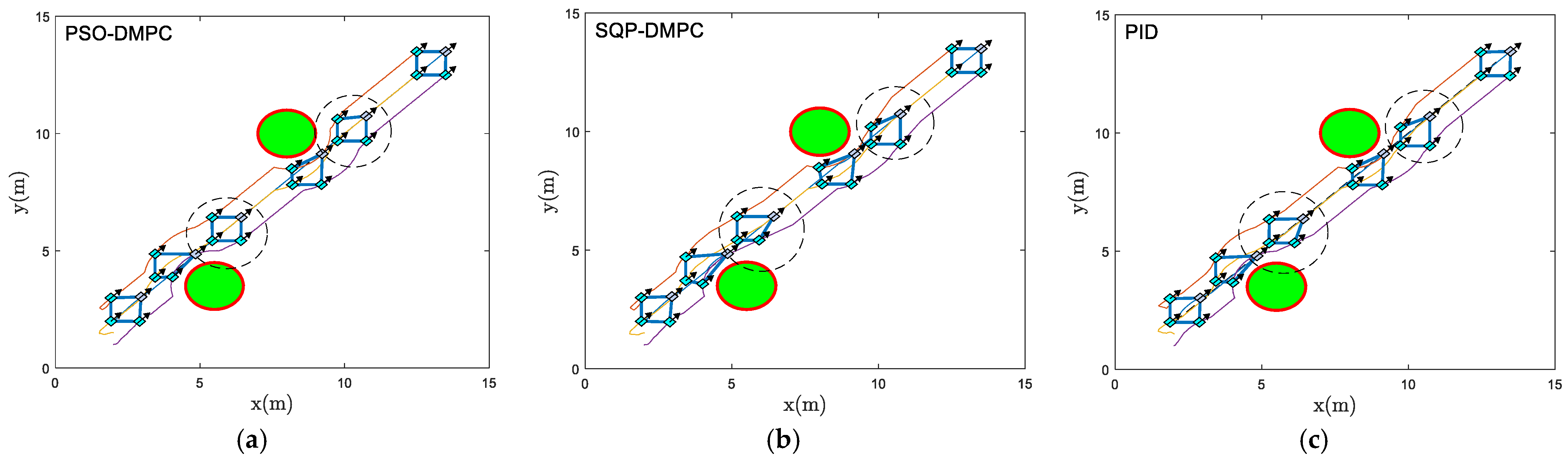
The formation trajectory-tracking results of example 1 using the traditional PID controller, the SQP-DMPC controller and PSO-DMPC controller in the x–y plane are presented in Figure 7. It can be seen that by implementing the PSO-DMPC, the formation is restored immediately after the obstacle avoidance is completed, while the SQP-DMPC and PID controllers have a transition process before restoring the initial formation. This is because PSO has a better processing ability for nonlinear obstacle avoidance and collision avoidance constraints with input limitation and has a stronger ability to find the global optimal solution. The relative distances of the three methods are presented in Figure 8. It can be seen from Figure 8 that the PSO-DMPC has the smallest mutual distance fluctuations when avoiding obstacles, which further shows that the quality of the optimal solution obtained via PSO is the best, and the deformation of the formation can be effectively reduced. The tracking performance along the x and y directions are shown in 
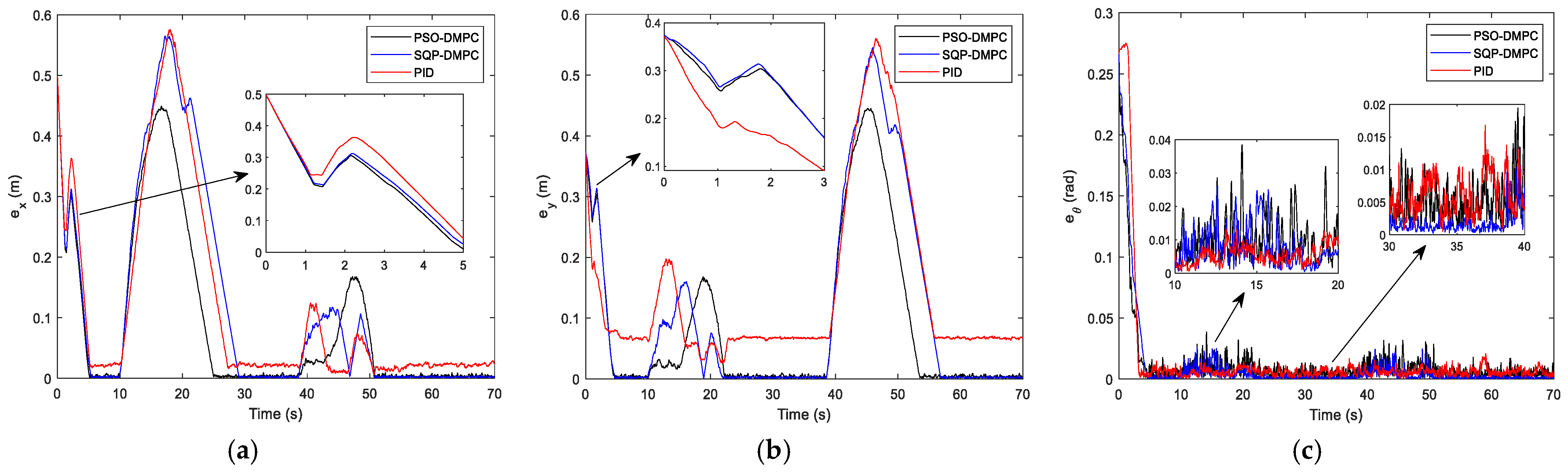
Figure 9a,b, respectively, and Figure 9c presents the heading angle tracking results of the MWMRs. It can be seen that the DMPC method has good tracking performance but that the PID controller has large steady-state tracking errors in the x and y coordinates. This is because the recede horizon optimization of the DMPC has a stronger ability to predict and correct nonlinear systems than the PID controller. The PSO-DMPC has a faster convergence rate than the SQP-DMPC and PID controllers. The RMS errors are show in Table 4. It can be observed that both the tracking error of the position and heading angle of the PSO-DMPC have the highest precision. The comparison of position consensus errors is presented in Figure 10. It can be observed that position consensus errors of the three methods converge to zero after about 2.5 s, and when avoiding obstacles, the PSO-DMPC have smaller consensus errors and faster formation convergence rates than the SQP-DMPC and PID controllers. The speeds of the MWMRs are shown in Figure 11.

4.2. Example 2 (Circle Line Formation Tracking)

In this example, a numerical simulation is performed further to test the ability to generate and maintain the desired formation with the time-varying heading angle using the proposed PSO-DMPC method. The desired formation shape is designed as an equilateral triangle with a side length of 1 m. Table 5 shows the initial states of three MWMRs. Table 6 shows the obstacle settings. The equation of the desired circle trajectory is given as:
{ x r = 7.5 + 5 cos 0.035 t y r = 7.5 + 5 sin 0.035 t θ r = π / 2 + 0.035 t
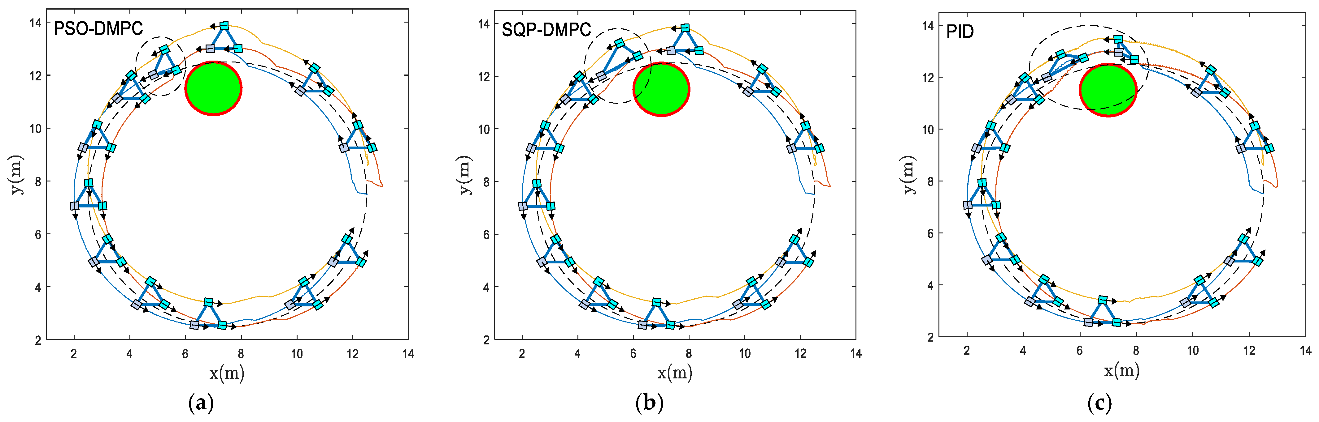
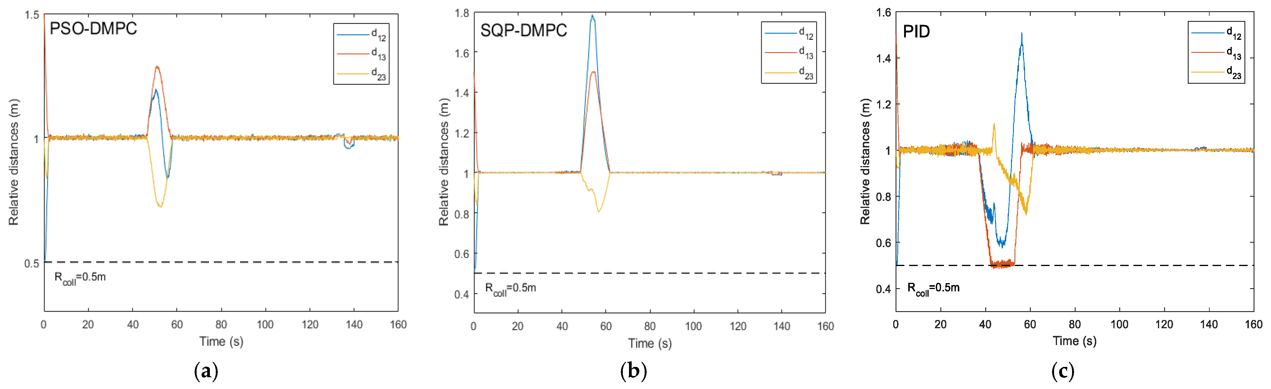
Figure 12 shows the formation trajectory-tracking results of the PSO-DMPC, SQP-DMPC, and traditional PID controller of example 2, and the relative distances of the MWMRs are shown in Figure 13. From Figure 12 and Figure 13, it can be seen that when the critical distance to the obstacle is reached, the formation deformations of the two DMPC methods are quite small, while the PID controller has a large formation deformation due to the insufficient ability to deal with constraints and disturbances. When PSO-DMPC ends the obstacle avoidance process, the SQP-DMPC and PID controllers still have larger formation deformation due to the insufficient ability to find global optimal solutions. The tracking performance along the x and y direction and the heading angle are shown in 
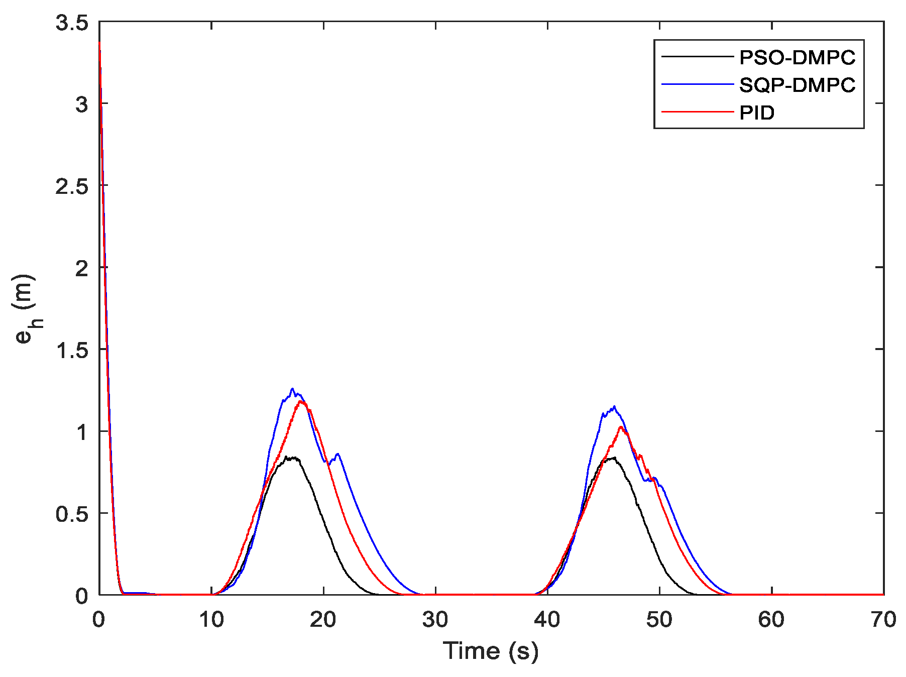
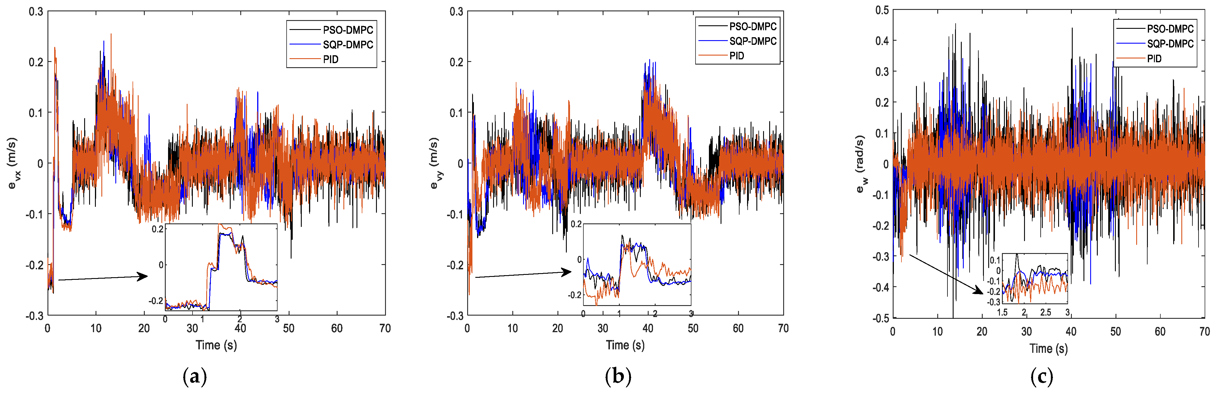
Figure 14a–c, respectively. It can be seen that the DMPC–based controller has a bigger tracking error when avoiding obstacles than the PID controllers but has a smaller tracking error during the formation maintaining process. To further illustrate the tracking performance, the RMS errors are show in Table 7. It can be observed that both the tracking error of the position and heading angle of the PSO-DMPC have the highest precision. The comparison of the position consensus errors is presented in Figure 15. It can be observed that all three methods have the capability of generating and maintaining the desired formation swiftly, and when avoiding obstacles, the PSO-DMPC has a smaller position consensus error and faster formation convergence rate than the SQP-DMPC and PID controllers. In Figure 16, the speeds of the MWMRs are shown.

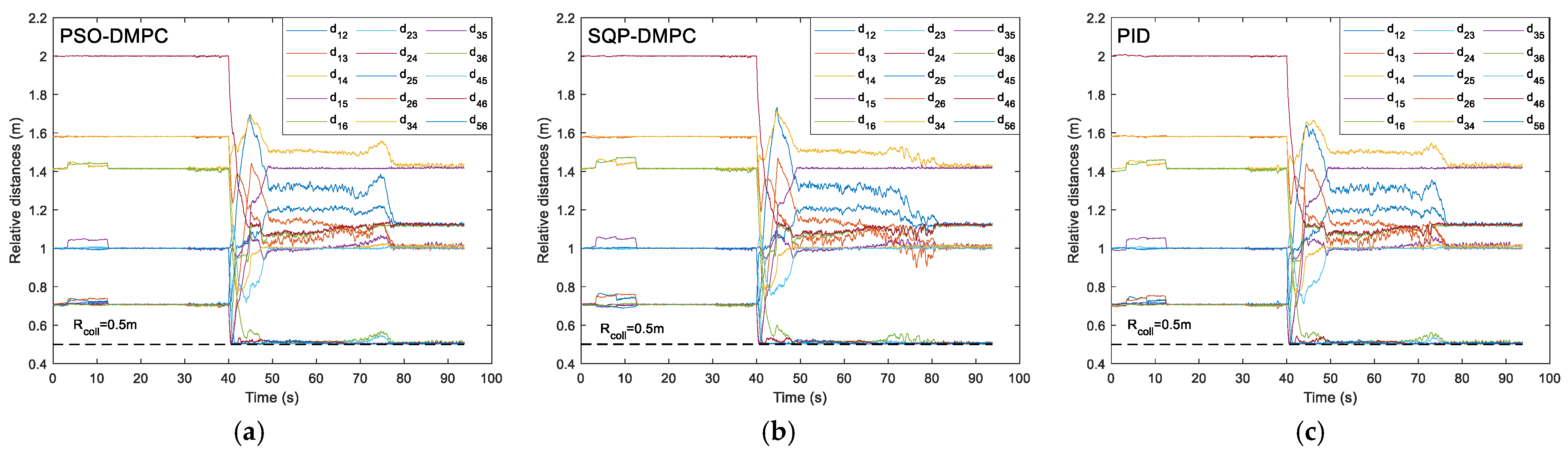
4.3. Example 3 (Curve Formation Tracking with Formation Reconstruction)

Example 3 is performed to test the formation maintenance and reconstruction ability of our proposed PSO-DMPC method. The desired trajectory is an irregular segmented trajectory containing two semicircles. The desired formation shape to be maintained is designed as an isosceles triangle with a bottom length of 2 m and a height length of 1 m. The desired formation shape to be reconstructed is designed as a rectangle with both the length and width as 1 m. Table 8 shows the initial states of six MWMRs. Table 9 shows the parameter settings of the obstacles.
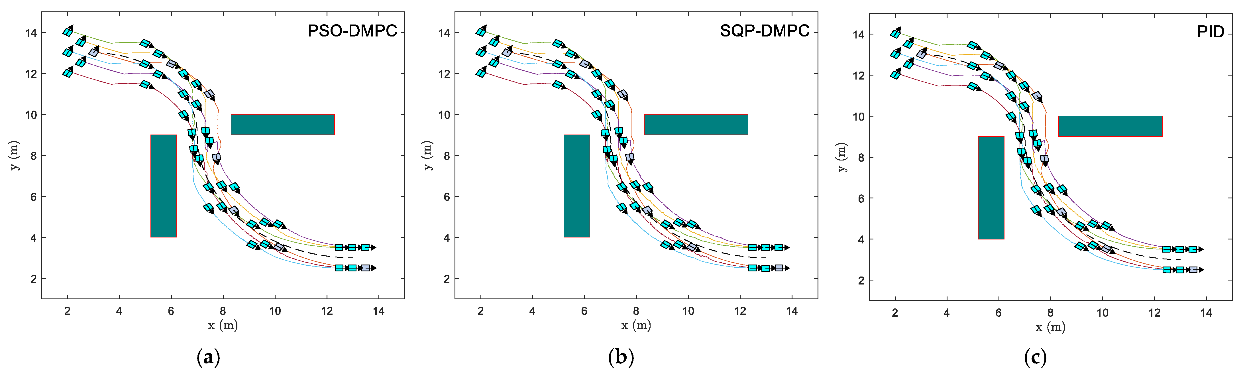
Figure 17 shows the formation trajectory-tracking results of the PSO-DMPC, SQP-DMPC, and traditional PID controller of example 3; we can see that the six MWMRs have good performance in generating, maintaining the desired formation, and tracking the desired trajectory. Figure 18 shows the relative distances between each of the two MWMRs in the formation. It can be found that the distances can maintain the desired initial values, and no collision between MWMRs occurs. 
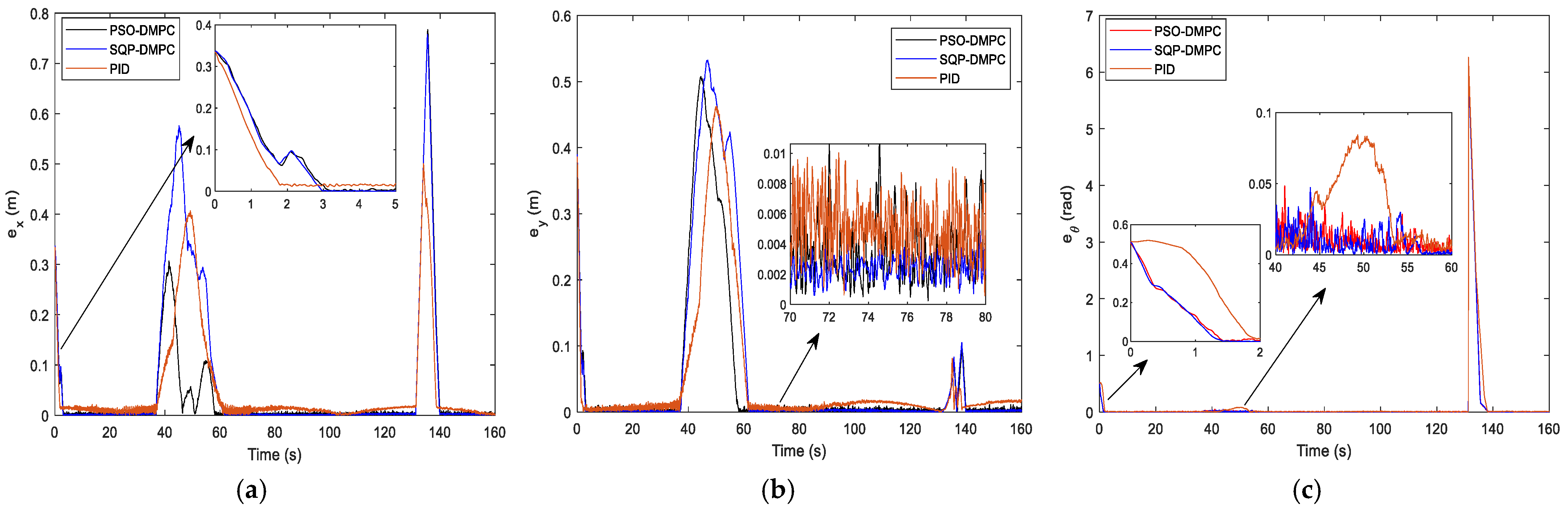
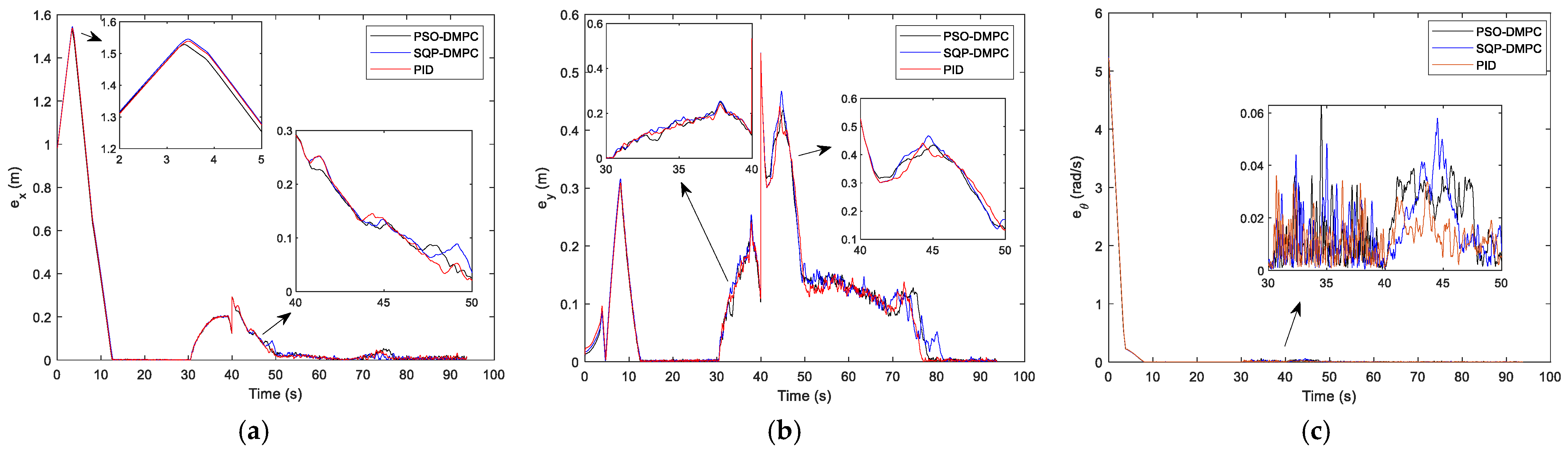
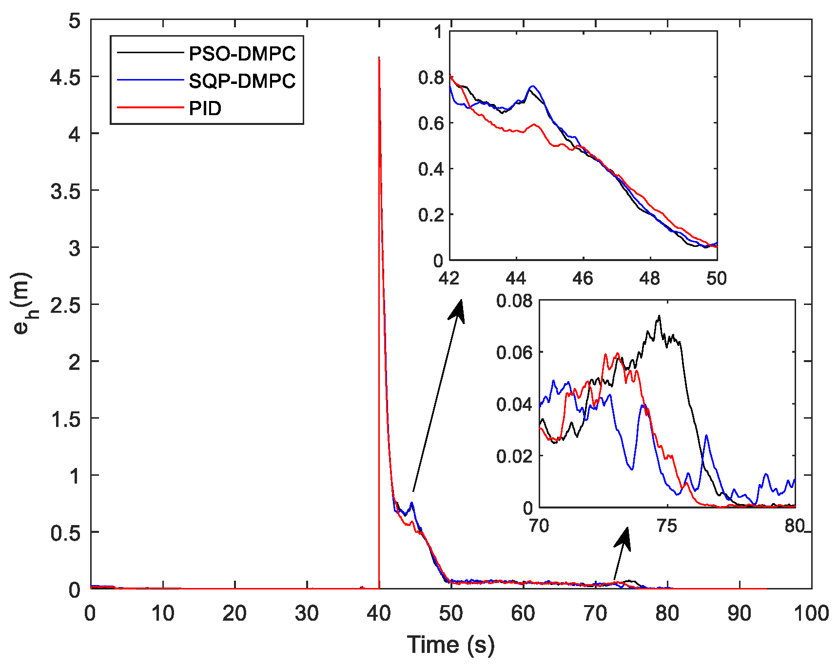
Figure 19a–c shows the tracking performance along the x and y direction and the heading angle, respectively. The comparison of the position consensus errors is presented in Figure 20. From Figure 19 and Figure 20, it can be seen that the three methods perform equally well. Therefore, to further illustrate the tracking performance, the RMS errors are show in Table 10. It can be observed that although the tracking error in the y direction of the PSO-DMPC controller is slightly less than that of the PID controller, both the tracking error of the x direction and heading angle of the PSO-DMPC have the highest precision. In 
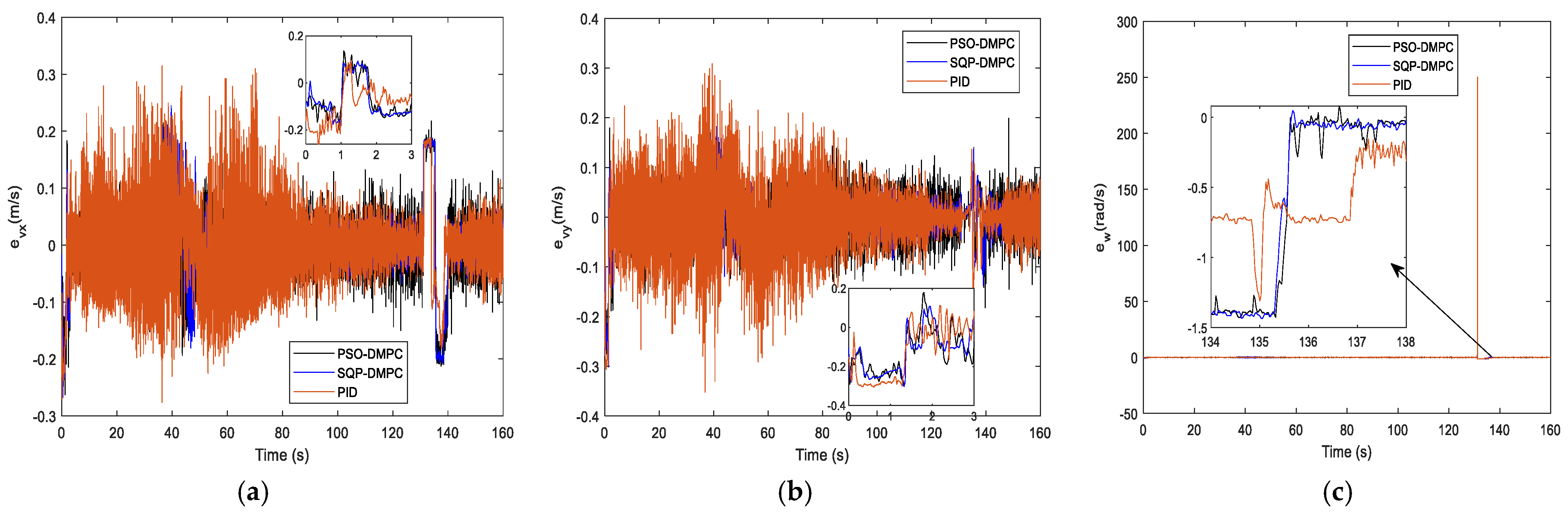
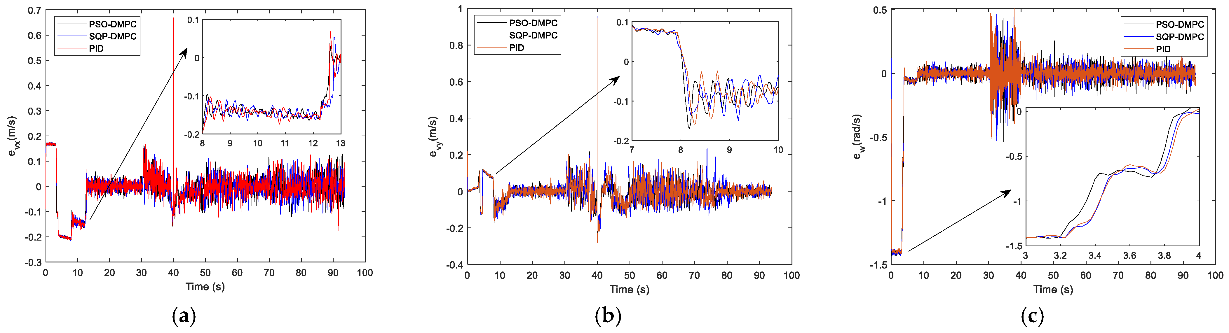
Figure 21 the speeds of the MWMRs are shown.
From the above simulation results, it can be concluded that the proposed PSO-DMPC controller has the better and more robust capability in terms of convergence time, tracking error, and consensus error than both the SQP-DMPC and PID controllers. Moreover, the simulation results also reflect the adaptability of the PSO-DMPC, which makes the designed closed-loop compensator have much better adaptive ability for the MWMRs in the presence of uncertainties and external disturbances. Therefore, the PSO-DMPC control method is effective and feasible for formation trajectory-tracking control of MWMRs with physical constraints and collision/obstacle avoidance simultaneously.

5. Conclusions

In this paper, the collision-free trajectory tracking formation control problem for multiple MWMRs under complexed obstacle environments via the DMPC scheme and real-time disturbance compensation is studied. The formation model for MWMRs is developed using a consensus strategy with the integrated kinematics and dynamics under the leader–follower framework. The DMPC scheme for the MWMRs’ formation is constructed, in which prediction information are shared among neighbors. Collision avoidance and obstacle avoidance are guaranteed by adding the penalty into the optimal control cost function. The constrained optimal control problems are solved online by the PSO algorithm. Then, the double closed-loop disturbance compensation controller is introduced to achieve real-time compensation for uncertainties and disturbances. Simulation results show that our proposed method can remove the effects of external disturbances and model uncertainties and achieve the formation trajectory-tracking with obstacle avoidance and collision avoidance accurately. Comparative studies indicate that the designed PSO-DMPC controller has better formation performance than the SQP-DMPC controller and the PID controller. Our future work will focus on the cooperative formation reconfiguration, including split and merge, under the unknown dynamic environment. In addition, the formation recursive self-healing and cooperative intent recognition under time-varying communication topology are also our following research interests.

Author Contributions

Conceptualization, X.Z.; software, T.Z.; data curation, T.Z.; writing—original draft preparation, T.Z.; writing—review and editing, X.Z. All authors have read and agreed to the published version of the manuscript.

Funding

This work is supported by National Natural Science Foundation of China (No. 61703012, 51975011).

Data Availability Statement

In this article, data sharing is not applicable as no datasets are generated or analyzed during the current study.

Conflicts of Interest

The authors declare no conflict of interest.

References

  1. Luo, X.; Mu, D.; Wang, Z.; Ning, P.; Hua, C. Adaptive full-state constrained tracking control for mobile robotic system with unknown dead-zone input. Neurocomputing 2023, 524, 31–42. [Google Scholar] [CrossRef]
  2. Zhang, J.; Li, S.; Meng, H.; Li, Z.; Sun, Z. Variable gain based composite trajectory tracking control for 4-wheel skid-steering mobile robots with unknown disturbances. Control Eng. Pract. 2023, 132, 105428. [Google Scholar] [CrossRef]
  3. Afaq, M.Z.; Jebelli, A.; Ahmad, R. An Intelligent Thermal Management Fuzzy Logic Control System Design and Analysis Using ANSYS Fluent for a Mobile Robotic Platform in Extreme Weather Applications. J. Intell. Robot. Syst. 2023, 107, 11. [Google Scholar] [CrossRef]
  4. Saenz, A.; Santibañez, V.; Bugarin, E.; Dzul, A.; Ríos, H.; Villalobos-Chin, J. Velocity control of an omnidirectional wheeled mobile robot using computed voltage control with visual feedback: Experimental results. Int. J. Control Autom. Syst. 2021, 19, 1089–1102. [Google Scholar] [CrossRef]
  5. Cao, G.; Zhao, X.; Ye, C.; Yu, S.; Li, B.; Jiang, C. Fuzzy adaptive PID control method for multi-mecanum-wheeled mobile robot. J. Mech. Sci. Technol. 2022, 36, 2019–2029. [Google Scholar] [CrossRef]
  6. Yuan, Z.; Tian, Y.; Yin, Y.; Wang, S.; Liu, J.; Wu, L. Trajectory tracking control of a four mecanum wheeled mobile platform: An extended state observer-based sliding mode approach. IET Control Theory Appl. 2020, 14, 415–426. [Google Scholar] [CrossRef]
  7. Chen, G.; Yao, D.; Zhou, Q.; Li, H.; Lu, R. Distributed event-triggered formation control of USVs with prescribed performance. J. Syst. Sci. Complex. 2022, 35, 820–838. [Google Scholar] [CrossRef]
  8. Moorthy, S.; Joo, Y.H. Distributed leader-following formation control for multiple nonholonomic mobile robots via bioinspired neurodynamic approach. Neurocomputing 2022, 492, 308–321. [Google Scholar] [CrossRef]
  9. Sanchez-Sanchez, A.G.; Hernandez-Martinez, E.G.; González-Sierra, J.; Ramírez-Neria, M.; Flores-Godoy, J.J.; Ferreira-Vazquez, E.D.; Fernandez-Anaya, G. Leader-Follower Power-based Formation Control Applied to Differential-drive Mobile Robots. J. Intell. Robot. Syst. 2023, 107, 6. [Google Scholar] [CrossRef]
  10. Wu, T.; Xue, K.; Wang, P. Leader-follower formation control of USVs using APF-based adaptive fuzzy logic nonsingular terminal sliding mode control method. J. Mech. Sci. Technol. 2022, 36, 2007–2018. [Google Scholar] [CrossRef]
  11. Zhen, Q.; Wan, L.; Li, Y.; Jiang, D. Formation control of a multi-AUVs system based on virtual structure and artificial potential field on SE (3). Ocean Eng. 2022, 253, 111148. [Google Scholar] [CrossRef]
  12. Hacene, N.; Mendil, B. Behavior-based autonomous navigation and formation control of mobile robots in unknown cluttered dynamic environments with dynamic target tracking. Int. J. Autom. Comput. 2021, 18, 766–786. [Google Scholar] [CrossRef]
  13. Lee, G.; Chwa, D. Decentralized behavior-based formation control of multiple robots considering obstacle avoidance. Intell. Serv. Robot. 2018, 11, 127–138. [Google Scholar] [CrossRef]
  14. Rauniyar, A.; Upreti, H.C.; Mishra, A.; Sethuramalingam, P. MeWBots: Mecanum-wheeled robots for collaborative manipulation in an obstacle-clustered environment without communication. J. Intell. Robot. Syst. 2021, 102, 1–18. [Google Scholar] [CrossRef]
  15. Mehrez, M.W.; Worthmann, K.; Cenerini, J.P.; Osman, M.; Melek, W.W.; Jeon, S. Model predictive control without terminal constraints or costs for holonomic mobile robots. Robot. Auton. Syst. 2020, 127, 103468. [Google Scholar] [CrossRef]
  16. Fu, M.; Wang, L. A fixed-time distributed formation control of marine surface vehicles with actuator input saturation and time-varying ocean currents. Ocean Eng. 2022, 251, 111067. [Google Scholar] [CrossRef]
  17. Liu, B.; Li, A.; Guo, Y.; Wang, C. Adaptive distributed finite-time formation control for multi-UAVs under input saturation without collisions. Aerosp. Sci. Technol. 2022, 120, 107252. [Google Scholar] [CrossRef]
  18. Alakshendra, V.; Chiddarwar, S.S. Adaptive robust control of mecanum-wheeled mobile robot with uncertainties. Nonlinear Dyn. 2017, 87, 2147–2169. [Google Scholar] [CrossRef]
  19. Sun, Z.; Hu, S.; Xie, H.; Li, H.; Zheng, J.; Chen, B. Fuzzy adaptive recursive terminal sliding mode control for an agricultural omnidirectional mobile robot. Comput. Electr. Eng. 2023, 105, 108529. [Google Scholar] [CrossRef]
  20. Yu, D.; Chen, C.P.; Xu, H. Fuzzy swarm control based on sliding-mode strategy with self-organized omnidirectional mobile robots system. IEEE Trans. Syst. Man Cybern. Syst. 2021, 52, 2262–2274. [Google Scholar] [CrossRef]
  21. Jin, X.; Wang, Z.; Zhao, J.; Yu, D. Swarm control for large-scale omnidirectional mobile robots within incremental behavior. Inf. Sci. 2022, 614, 35–50. [Google Scholar] [CrossRef]
  22. Lu, X.; Zhang, X.; Zhang, G.; Fan, J.; Jia, S. Neural network adaptive sliding mode control for omnidirectional vehicle with uncertainties. ISA Trans. 2019, 86, 201–214. [Google Scholar] [CrossRef] [PubMed]
  23. Zhao, T.; Zou, X.; Dian, S. Fixed-time observer-based adaptive fuzzy tracking control for Mecanum-wheel mobile robots with guaranteed transient performance. Nonlinear Dyn. 2022, 107, 921–937. [Google Scholar] [CrossRef]
  24. Wang, D.; Wei, W.; Wang, X.; Gao, Y.; Li, Y.; Yu, Q.; Fan, Z. Formation control of multiple mecanum-wheeled mobile robots with physical constraints and uncertainties. Appl. Intell. 2022, 52, 2510–2529. [Google Scholar] [CrossRef]
  25. Tsai, C.C.; Wu, H.L.; Tai, F.C.; Chen, Y.S. Distributed consensus formation control with collision and obstacle avoidance for uncertain networked omnidirectional multi-robot systems using fuzzy wavelet neural networks. Int. J. Fuzzy Syst. 2017, 19, 1375–1391. [Google Scholar] [CrossRef]
  26. Mu, C.; Peng, J. Learning-based cooperative multiagent formation control with collision avoidance. IEEE Trans. Syst. Man Cybern. Syst. 2022, 52, 7341–7352. [Google Scholar] [CrossRef]
  27. Hwang, J.; Lee, J.; Park, C. Collision avoidance control for formation flying of multiple spacecraft using artificial potential field. Adv. Space Res. 2022, 69, 2197–2209. [Google Scholar] [CrossRef]
  28. Barghandan, M.; Pirmohamadi, A.A.; Mobayen, S.; Fekih, A. Optimal adaptive barrier-function super-twisting nonlinear global sliding mode scheme for trajectory tracking of parallel robots. Heliyon 2023, 9, e13378. [Google Scholar] [CrossRef]
  29. Alattas, K.A.; Vu, M.T.; Mofid, O.; El-Sousy, F.F.; Fekih, A.; Mobayen, S. Barrier function-based nonsingular finite-time tracker for quadrotor UAVs subject to uncertainties and input constraints. Mathematics 2022, 10, 1659. [Google Scholar] [CrossRef]
  30. Li, J.; Wang, Q.; Su, Y.; Sun, C. Robust distributed model predictive consensus of discrete-time multi-agent systems: A self-triggered approach. Front. Inf. Technol. Electron. Eng. 2021, 22, 1068–1079. [Google Scholar] [CrossRef]
  31. Li, S.; Ye, D.; Xiao, Y.; Sun, Z. Robust distributed model predictive control for satellite cluster reconfiguration with collision avoidance. Aerosp. Sci. Technol. 2022, 130, 107917. [Google Scholar] [CrossRef]
  32. Zhao, R.; Miao, M.; Lu, J.; Wang, Y.; Li, D. Formation control of multiple underwater robots based on ADMM distributed model predictive control. Ocean Eng. 2022, 257, 111585. [Google Scholar] [CrossRef]
  33. Rosenfelder, M.; Ebel, H.; Eberhard, P. Cooperative distributed nonlinear model predictive control of a formation of differentially-driven mobile robots. Robot. Auton. Syst. 2022, 150, 103993. [Google Scholar] [CrossRef]
  34. Qin, D.; Liu, A.; Zhang, D.; Ni, H. Formation control of mobile robot systems incorporating primal-dual neural network and distributed predictive approach. J. Frankl. Inst. 2020, 357, 12454–12472. [Google Scholar] [CrossRef]
  35. Xiao, H.; Yu, D.; Chen, C.P. Self-triggered-organized mecanum-wheeled robots consensus system using model predictive based protocol. Inf. Sci. 2022, 590, 45–59. [Google Scholar] [CrossRef]
  36. Diwan, S.P.; Deshpande, S.S. Fast nonlinear model predictive controller using parallel PSO based on divide and conquer approach. Int. J. Control 2022, 96, 1–10. [Google Scholar] [CrossRef]
  37. Hong, S.H.; Ou, J.; Wang, Y. Physics-guided neural network and GPU-accelerated nonlinear model predictive control for quadcopter. Neural Comput. Appl. 2022, 35, 393–413. [Google Scholar] [CrossRef]
  38. Amouri, A.; Cherfia, A.; Merabti, H.; Laib, D.L.Y. Nonlinear model predictive control of a class of continuum robots using kinematic and dynamic models. FME Trans. 2022, 50, 339–350. [Google Scholar] [CrossRef]
  39. Fan, W.; Hu, Z.; Veerasamy, V. PSO-Based Model Predictive Control for Load Frequency Regulation with Wind Turbines. Energies 2022, 15, 8219. [Google Scholar] [CrossRef]
  40. Abdolahi, Y.; Yousefi, S.; Tavoosi, J. A New Self-Tuning Nonlinear Model Predictive Controller for Autonomous Vehicles. Complexity 2023, 2023, 8720849. [Google Scholar] [CrossRef]
  41. Kapnopoulos, A.; Alexandridis, A. A cooperative particle swarm optimization approach for tuning an MPC-based quadrotor trajectory tracking scheme. Aerosp. Sci. Technol. 2022, 127, 107725. [Google Scholar] [CrossRef]
  42. Guo, L.; Liu, H.; Han, L.; Yang, N.; Liu, R.; Xiang, C. Predictive energy management strategy of dual-mode hybrid electric vehicles combining dynamic coordination control and simultaneous power distribution. Energy 2023, 263, 125598. [Google Scholar] [CrossRef]
  43. Sun, S.; Romero, A.; Foehn, P.; Kaufmann, E.; Scaramuzza, D. A comparative study of nonlinear mpc and differential-flatness-based control for quadrotor agile flight. IEEE Trans. Robot. 2022, 38, 3357–3373. [Google Scholar] [CrossRef]
  44. Nan, F.; Sun, S.; Foehn, P.; Scaramuzza, D. Nonlinear MPC for quadrotor fault-tolerant control. IEEE Robot. Autom. Lett. 2022, 7, 5047–5054. [Google Scholar] [CrossRef]
  45. Ghandriz, T.; Jacobson, B.; Nilsson, P.; Laine, L. Trajectory-following and off-tracking minimisation of long combination vehicles: A comparison between nonlinear and linear model predictive control. Veh. Syst. Dyn. 2023, 61, 1–34. [Google Scholar] [CrossRef]
  46. Han, J.; Shan, X.; Liu, H.; Xiao, J.; Huang, T. Fuzzy gain scheduling PID control of a hybrid robot based on dynamic characteristics. Mech. Mach. Theory 2023, 184, 105283. [Google Scholar] [CrossRef]
  47. Yu, X.; Fan, Y.; Xu, S.; Ou, L. A self-adaptive SAC-PID control approach based on reinforcement learning for mobile robots. Int. J. Robust Nonlinear Control 2022, 32, 9625–9643. [Google Scholar] [CrossRef]
  48. Shojaei, K. A prescribed performance PID control of robotic cars with only posture measurements considering path curvature. Eur. J. Control 2022, 65, 100616. [Google Scholar] [CrossRef]
Figure 1. Abridged general view of the MWMR.
Actuators 12 00127 g001
Figure 2. Diagram of MWMR formation trajectory tracking.
Actuators 12 00127 g002
Figure 3. General framework of DMPC for MWMR formation.
Actuators 12 00127 g003
Figure 4. Collision and obstacle avoidance for MWMRs.
Actuators 12 00127 g004
Figure 5. Framework of PSO-based DMPC scheme.
Actuators 12 00127 g005
Figure 6. Disturbance feedback compensation structure.
Actuators 12 00127 g006
Figure 7. Formation trajectories of different control methods (Example 1). (a) PSO-DMPC, (b) SQP-DMPC and (c) PID.
Actuators 12 00127 g007
Figure 8. Distances between MWMRs of different control methods (Example 1). (a) PSO-DMPC, (b) SQP-DMPC, and (c) PID.
Actuators 12 00127 g008
Figure 9. Trajectory tracking error of (a) x direction, (b) y direction, and (c) heading angle (Example 1).
Actuators 12 00127 g009
Figure 10. Position consensus error (Example 1).
Actuators 12 00127 g010
Figure 11. Speed error of (a) x direction, (b) y direction, and (c) angular velocity. (Example 1).
Actuators 12 00127 g011
Figure 12. Formation trajectories of different control methods (Example 2). (a) PSO-DMPC, (b) SQP-DMPC, and (c) PID.
Actuators 12 00127 g012
Figure 13. Distances between MWMRs of different control methods (Example 2). (a) PSO-DMPC, (b) SQP-DMPC and (c) PID.
Actuators 12 00127 g013
Figure 14. Trajectory tracking error of (a) x direction, (b) y direction, and (c) heading angle (Example 2).
Actuators 12 00127 g014
Figure 15. Position consensus error (Example 2).
Actuators 12 00127 g015
Figure 16. Speed error of (a) x direction, (b) y direction, and (c) angular velocity (Example 2).
Actuators 12 00127 g016
Figure 17. Formation trajectories of different control methods (Example 3). (a) PSO-DMPC, (b) SQP-DMPC and (c) PID.
Actuators 12 00127 g017
Figure 18. Distances between MWMRs of different control methods (Example 3). (a) PSO-DMPC, (b) SQP-DMPC and (c) PID.
Actuators 12 00127 g018
Figure 19. Trajectory tracking error of (a) x direction, (b) y direction, and (c) heading angle (Example 3).
Actuators 12 00127 g019
Figure 20. Position consensus error (Example 3).
Actuators 12 00127 g020
Figure 21. Speed error of (a) x direction, (b) y direction, and (c) angular velocity (Example 3).
Actuators 12 00127 g021
Table 1. Parameter values of the multi-robot formation system.
DefinitionSymbolValueUnit
Mass of robotsm5kg
Sampling period t s 0.025s
Radius of wheelsRw0.05m
Moment of inertia of robotsJz0.01875kg·m2
Moment of inertia of wheelsJw0.000625kg·m2
Longitudinal distance of wheels to centera0.145m
Lateral distance of wheels to centerb0.145m
Viscous friction coefficient of wheels λ i 0.2None
Static friction coefficient of wheels μ 0.1None
Table 2. Initial states of four MWMRs (Example 1).
MWMR(x, y) (m)θ (rad)(vx, vy) (m/s)w (rad/s)
MWMR-1(2, 2) π / 3 (1, 1) π / 4
MWMR-2(2, 3) π / 3 (1, 1) π / 4
MWMR-3(2, 1.5) π / 3 (1, 1) π / 4
MWMR-4(2, 1) π / 3 (1, 1) π / 4
Table 3. Parameter settings of obstacles (Example 1).
ObstaclePosition (m)Ro (m)
Obstacle-1(5.5, 3.5)1
Obstacle-2(8, 10)1
Table 4. RMS values of tracking error for example 1. (unit: m).
RMS ValuePIDSQP-MPCPSO-MPC
| | e x | | R M S 0.11660.12000.0883
| | e y | | R M S 0.14480.11020.0845
| | e θ | | R M S 0.01450.01030.0125
Table 5. Initial states of three MWMRs (Example 2).
MWMR(x, y) (m)θ (rad)(vx, vy) (m/s)w (rad/s)
MWMR-1(12.5, 7.5) π / 3 (1, 1) π / 4
MWMR-2(12.5, 8) π / 3 (1, 1) π / 4
MWMR-3(12.5, 9) π / 3 (1, 1) π / 4
Table 6. Parameter settings of the obstacle (Example 2).
ObstaclePosition (m)Ro (m)
Obstacle-1(7, 11.5)1
Table 7. RMS values of tracking error for example 2. (unit: m).
RMS ValuePIDSQP-MPCPSO-MPC
| | e x | | R M S 0.05130.06730.0408
| | e y | | R M S 0.04600.05750.0458
| | e θ | | R M S 0.11350.09220.0881
Table 8. Initial states of six MWMRs (Example 3).
MWMR(x, y) (m)θ (rad)(vx, vy) (m/s)w (rad/s)
MWMR-1(3, 13) π / 3 (1, 1) π / 4
MWMR-2(2.5, 13.5) π / 3 (1, 1) π / 4
MWMR-3(2.5, 12.5) π / 3 (1, 1) π / 4
MWMR-4(2, 14) π / 3 (1, 1) π / 4
MWMR-5(2, 13) π / 3 (1, 1) π / 4
MWMR-6(2, 12) π / 3 (1, 1) π / 4
Table 9. Parameter settings of the obstacles (Example 3).
ObstaclePosition (m)Length (m)Width (m)
Obstacle-1(5.3, 4)15
Obstacle-2(8.3, 9)41
Table 10. RMS values of tracking error for example 3. (unit: m).
RMS ValuePIDSQP-MPCPSO-MPC
| | e x | | R M S 0.15360.15520.1531
| | e y | | R M S 0.09740.10190.0989
| | e θ | | R M S 0.11990.12080.1188
Disclaimer/Publisher’s Note: The statements, opinions and data contained in all publications are solely those of the individual author(s) and contributor(s) and not of MDPI and/or the editor(s). MDPI and/or the editor(s) disclaim responsibility for any injury to people or property resulting from any ideas, methods, instructions or products referred to in the content.

