Mechanism Analysis and Control of Lateral Instability of 4WID Vehicle Based on Phase Plane Analysis Considering Front Wheel Angle

Abstract

The current vehicle stability judgment methods in the stability control of distributed drive electric vehicles focuses on using the phase plane method, but the existing phase plane stability boundary delineation methods ignore the influence of the front wheel rotation angle. Therefore, a new phase plane partitioning method (NPPPM) is proposed in this paper, and a new phase plane stability domain library is established. Based on this, the direct yaw moment control of distributed drive electric vehicle through phase plane analysis is established. Firstly, the influence of the front wheel turning angle on the phase plane is considered in the design of the phase plane stability boundary, and a new stability boundary function is fitted by the least squares method. This approach avoids the lateral instability caused by too large a front-wheel turning angle and improves the accuracy of vehicle stability judgment. Next, a hierarchical direct transverse moment controller is constructed using Matlab/Simulink. Among them, the upper layer controller adopts sliding mode control with the sideslip angle error of the center of mass as the tracking target. The lower controller adopts the optimal configuration algorithm with the optimal road adhesion utilization as the objective function. Finally, the effectiveness and superiority of the proposed phase plane partitioning method (NPPPM) for distributed drive electric vehicles with sinusoidal and angular order inputs for the front wheel rotation angle are verified by simulation.

1. Introduction

Electric vehicles are currently the focus of scholarly research due to their advantages in terms of energy efficiency and environmental protection. In the development process of distributed drive electric vehicle, the vehicle driven by a four-wheel hub motor plays a milestone role. It can make good use of the drive and braking torque from the wheel hub motors to enhance the control of the vehicle. Meanwhile, the distributed drive electric vehicle eliminates the drive shaft and transmission components, simplifies the chassis structure of the vehicle, improves the space utilization rate of the vehicle, achieves the purpose of being lightweight, and, thus, reduces energy consumption [1,2,3]. At the same time, the distributed hub motor drive vehicle eliminates the complex transmission mechanism, and the driver’s operation can be quickly transferred to the hub motor, which improves the control speed and accuracy. However, the distributed drive electric vehicles driven by hub motors, due to the larger mass of hub motor, will lead to increased difficulty in lateral stability control when the vehicle occurs yaw and sideslip, so the distributed drive electric vehicle lateral stability control research has become indispensable in the research of new energy vehicles [4,5,6,7,8].

In recent years, the research on stability control of distributed drive electric vehicles mainly focuses on two aspects. One is how to determine whether the vehicle is unstable. The second one is how to reasonably use modern control theory and an optimization algorithm to accurately distribute torque to the four hub motors in order to achieve the purpose of a stable vehicle running state.

At present, there are two main research methods to determine whether the vehicle is unstable. The first method is to use the linear two-degree-of-freedom vehicle dynamics model to calculate the ideal yaw rate and sideslip angle and take them as the ideal variation for tracking control. The second one is to study the stability of the vehicle by establishing the phase plane of the yaw rate and sideslip angle [9,10,11,12]. In terms of stability control, most scholars at home and abroad are limited to stability control under normal braking conditions, and lateral stability control under extreme conditions is less researched.

At present, some scholars have systematically analyzed the instability mechanism of vehicles based on Lyapunov’s first method and phase plan [13,14]. Some scholars also established a phase diagram based on the ratio of steering kinetic energy to forward kinetic energy through longitudinal and transverse energy analysis [15]. Sadri and Wu et al. [16,17,18] used Lyapunov direct method to analyze vehicle stability and proposed two Lyapunov functions independent of vehicle parameters. The stability boundary was estimated, and the influence of vehicle speed, road adhesion coefficient, and the front wheel angle on the stability region was studied. Some scholars used the energy method to derive the formula of vehicle instability kinetic energy and longitudinal kinetic energy and defined the agreement between the two as instability energy ratio. On this basis, a vehicle stability criterion based on the phase plane method was proposed to judge vehicle stability [19,20]. Wei Liu and Lu Xiong et al. divided the types of phase plane stable boundary into diamond stable boundary and curve stable boundary. The stable boundary of the curve is fitted by a quartic polynomial. However, the paper did not mention the functional relationship between the stable boundary and the front wheel angle, longitudinal speed, and road adhesion coefficient [21]. Liu Jun et al. proposed to adopt a linear method to divide the lateral declination angle of the center of mass and yaw rate phase into planes, which would lead to the reduction of the stability region. Although it can improve the stability of the vehicle, it will reduce the comfort of the driver to a certain extent [22]. Liu Xuecheng et al. proposed to divide the stable region of the phase plane in the form of broken lines, but the control in the stable region was not mentioned [23]. Fei Lai et al. [24] analyzed the lateral declination angle of the center of mass—lateral declination velocity phase plane on the uneven road surface, based on a unified longitudinal and transverse dynamic model. However, the author assumes that the uneven road surface is a continuous wavy type and that the influence of the road surface on the four wheels is consistent, which is not consistent in the actual situation. Huang Long [25] proposed that the stable boundary coefficient is related to the road adhesion coefficient, and the stable boundary coefficient remains unchanged in a certain range of road adhesion coefficient. However, this method does not consider the speed and the front wheel angle, so the reliability is low.

In terms of vehicle control, Zhong Longfei et al. [26] established the stability domain boundary model of vehicle centroid side deflection angle phase plane under different road adhesion coefficients and proposed that the distance from the unstable point to the stable boundary was the instability degree, and fuzzy neural network was used to control the direct yaw moment. Li Xiaoyu [9] used the front and rear wheel side angle $\left({\alpha }_f-{\alpha }_r\right)$ phase plane to describe the stability of a vehicle driven by a four-wheel hub motor under compound conditions. He proposed a vehicle state observer based on the fusion of the kinematic model and dynamic model. Finally, model predictive control was used to improve the driving stability of the vehicle. Xiao Feng [27] designed a method based on the distance between the state point and the stable boundary to measure the vehicle stability index and improve the driving stability of the vehicle through direct yaw moment control. Mengxiong Lu [28] designed a dual sliding mode control of active front-wheel steering (AFS) and direct yaw moment (DYC), which further improved the lateral stability of the vehicle. Gong Tianyang et al. [29] designed a fuzzy control method, which takes the errors of yaw rate and sideslip angle as tracking targets, outputs additional yaw moment and rear wheel angle, and uses a genetic algorithm to optimize the membership function of fuzzy control. Yitong Song [30] proposed the estimation method of tire lateral force and vehicle sideslip angle based on an odorless Kalman filter and proposed a hierarchical control strategy where the upper controller is the sliding mode control and the lower controller is the optimal distribution controller, which improves the vehicle handling stability and energy efficiency. However, the nonlinear characteristics of vehicle motion cannot be avoided by using simple sliding mode control. Hongwei Wang et al. [31] proposed a vehicle lateral stability controller based on integral sliding mode control and optimal allocation. By adding an exponential term to the traditional approach rate, the smooth transition of the sliding mode surface is realized, and the effect of buffeting is reduced. Xiaoqiang Sun et al. [32] proposed a method based on non-singular terminal sliding mode control for direct yaw moment control of distributed drive electric vehicles. This method can effectively avoid the nonlinear characteristics of vehicle motion. However, the stability region division of the phase plane does not take into account the influence of the front wheel angle.

In summary, a new phase plane partitioning method (NPPPM) is proposed, and the phase plane stability domain library is established on this basis. In the process of designing the phase plane stable boundary, the stable boundary function about the front wheel angle is designed, which avoids the situation that the phase plane stable boundary changes little when the front wheel angle changes in the past. The lateral stability of the vehicle with sinusoidal input and angular step input is verified by the layered direct yaw moment control. The upper layer is controlled by sliding mode, and the error of the centroid side deflection angle is the tracking target. The lower controller is the optimal allocation and takes the optimal road adhesion utilization rate as the objective function. Finally, the effectiveness of the proposed phase plane division method (NPPPM) is verified by simulation under sinusoidal and angular step input conditions of the front wheel angle.

This paper consists of six parts. The first part introduces the research background and motivation for this paper. The Section 2 introduces the dynamic model of distributed drive electric vehicle. The Section 3 introduces the mechanism of lateral instability of vehicle based on phase plane analysis and the establishment of a phase plane stability domain library. The fourth part is the construction of the layered direct yaw control system. In Section 5, the stability performance of the vehicle under the same working conditions is evaluated by using the NPPPM method and OPPPM method, respectively, and the simulation results are given. Finally, the conclusion is given in the last section.

2. Distributed Drive Electric Vehicle Dynamics Model

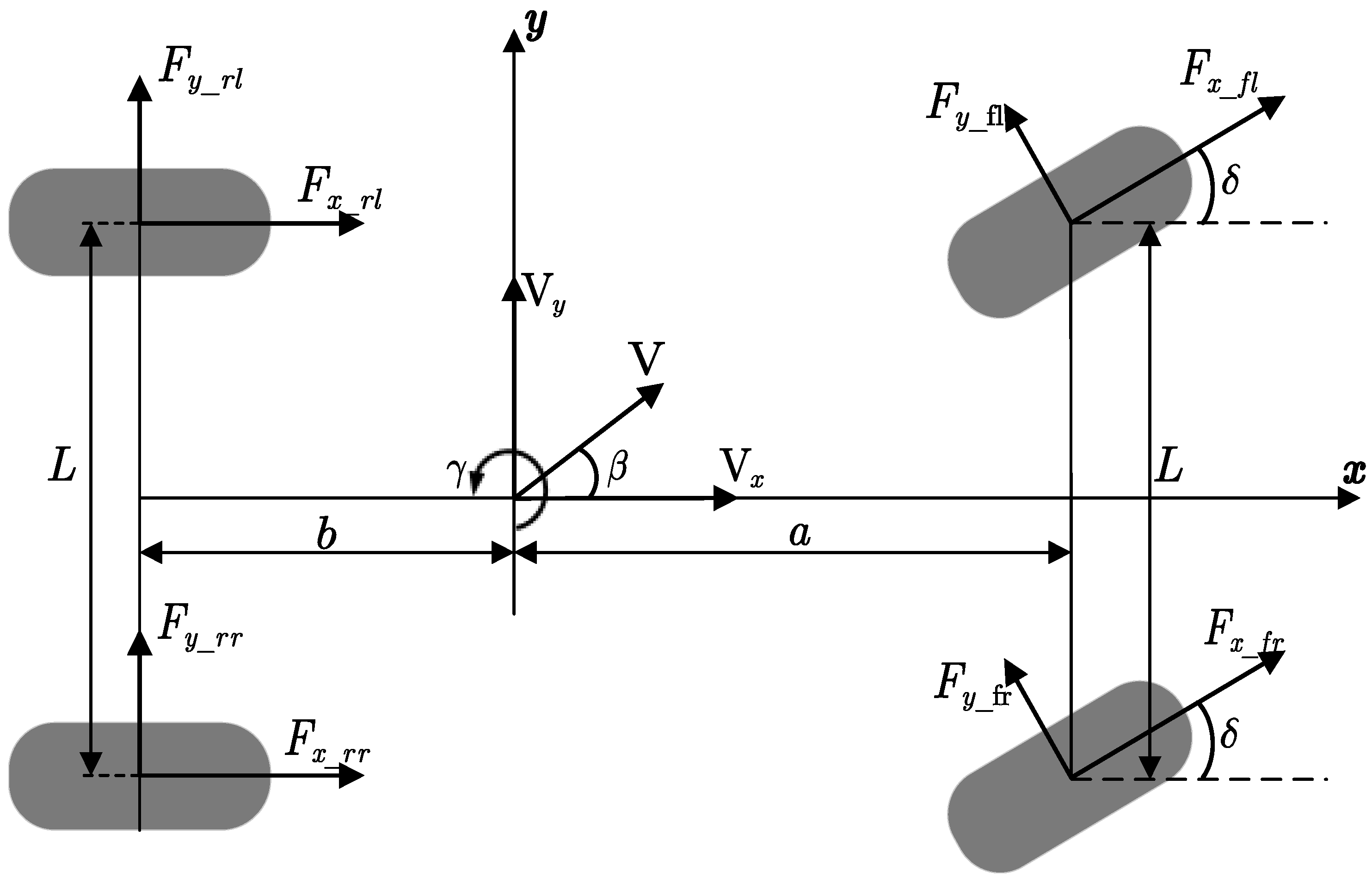
2.1. Distributed Drive Vehicle Seven-Degree-of-Freedom Dynamics Model

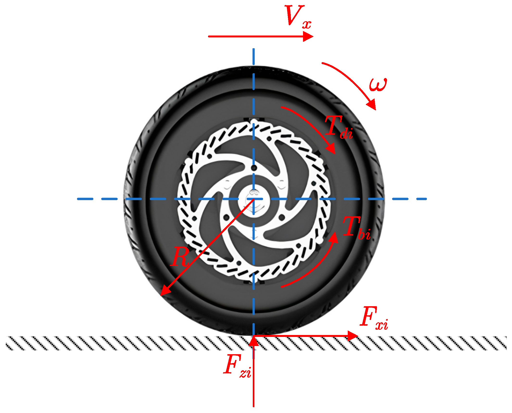
In this paper, the body dynamics of the vehicle in three directions, longitudinal, lateral, and yaw, were established using Newton–Euler theory, as shown in Figure 1.

To comply with the assumption of consistent front wheel angles in the ideal model of a two-degree-of-freedom vehicle below, we assume in our study that the left and right front wheel angles are equal in a seven-degree-of-freedom vehicle model. This assumption, known as the front wheel cell assumption, is commonly used in simplified vehicle dynamic models to reduce complexity and computational effort. When the speed of the vehicle in the longitudinal direction is constant, then the equations for the longitudinal, lateral, and yaw movements of the vehicle are as follows:

$$\sum F_x=m\left({\dot{V}}_x-V_y\gamma \right)=\left(F_{x\_fl}+F_{x\_fr}\right)\mathrm{c}\mathrm{o}\mathrm{s}\delta +F_{x\_rl}+F_{x\_rr}-\left(F_{y\_fl}+F_{y\_fr}\right)\mathrm{s}\mathrm{i}\mathrm{n}\delta$$

(1)

$$\sum F_y=m\left({\dot{V}}_y+V_x\gamma \right)=\left(F_{y\_fl}+F_{y\_fr}\right)\mathrm{c}\mathrm{o}\mathrm{s}\delta +F_{y\_rl}+F_{y\_rr}+\left(F_{x\_fl}+F_{x\_fr}\right)\mathrm{s}\mathrm{i}\mathrm{n}\delta$$

(2)

$$\sum M=I_z\dot{\gamma }=a\left[\left(F_{x\_fl}+F_{x\_fr}\right)\mathrm{s}\mathrm{i}\mathrm{n}\delta +\left(F_{y\_fl}+F_{y\_fr}\right)\mathrm{c}\mathrm{o}\mathrm{s}\delta \right]-b\left(F_{y\_rl}+F_{y\_rr}\right)+\frac{1}{2}L\left[\left(F_{y\_fr}-F_{y\_fl}\right)\mathrm{s}\mathrm{i}\mathrm{n}\delta +\left(F_{x\_fr}-F_{x\_fl}\right)\mathrm{c}\mathrm{o}\mathrm{s}\delta \right]+\frac{1}{2}L\left(F_{x\_rl}-F_{x\_rr}\right)$$

(3)

In the above equation, $m$ is the overall vehicle mass, $I_z$ is the vehicle moment of inertia, $\gamma$ is the vehicle yaw rate, and $\delta$ represents the front wheel angle. In order to conform to the ideal model of a two-degree-of-freedom vehicle presented below, we make the assumption that the turning angles of the left and right front wheels are identical. $V_x$ is the vehicle longitudinal velocity, and $V_y$ is the vehicle lateral velocity. $V$ is the vehicle center of mass velocity, $L$ is the wheelbase, $a$ is the distance from the centre of mass to the front axle, $b$ is the distance from the center of mass to the rear axle, $F_{x\_ij}$ is the longitudinal force at each wheel, and $F_{y\_ij}$ is the lateral force per wheel. Vehicle parameters as shown in

Table 1. Vehicle parameters.

Description	Symbol	Value
Total mass of the car vehicle	m	1560 (kg)
Distance from front axle to the center of centroid	a	1.617 (m)
Distance from rear axle to the center of centroid	b	1.683 (m)
Moment of inertia of the wheel	J	2.1 ($\mathrm{k}\mathrm{g}·{\mathrm{m}}^2$)
Yaw moment of inertia of vehicle	$I_z$	1523 ($\mathrm{k}\mathrm{g}·{\mathrm{m}}^2$)
Distance from the center of centroid to ground	h	0.556 (m)
Track width	L	1.82 (m)
Rolling radius of the tire	R	0.354 (m)
Front wheel cornering stiffness	$k_f$	16,000 (N/rad)
Rear wheel cornering stiffness	$k_r$	16,000 (N/rad)
Rolling resistance coefficient	f	0.015

.

2.2. Wheel Models

The mechanical analysis of the wheels during vehicle travel is shown in Figure 2 where the differential equation for the four-wheel moments of a distributed drive electric vehicle can be expressed as follows:

$$J{\dot{\omega }}_i=-T_{bi}+T_{di}-F_{xi}R$$

(4)

where $J$ is the rotational moment of inertia of the wheel, ${\dot{\omega }}_i$ is the angular acceleration of the vehicle rotation, $T_{bi}$ is the wheel braking torque, $T_{di}$ is the wheel driving torque, $F_{xi}$ is the longitudinal force of the tire, and $R$ is the tire radius.

2.3. Magic Formula Tyre Model

In this paper, the Magic Formula tire model is used as an empirical model to represent the tire forces as a combination of trigonometric functions. It can directly reflect the mathematical relationship between the input variables: side slip angle of the tire, slip rate of the tire, and the output variables: tire longitudinal force; tire lateral force; and return torque. When $x$ is the side slip angle, $F\left(x\right)$ is sought as the lateral force; when $x$ is the slip rate, $F\left(x\right)$ is sought as the longitudinal force. The general expressions are as follows:

$$F\left(x\right)=D\mathrm{s}\mathrm{i}\mathrm{n}\left\{C\mathrm{a}\mathrm{r}\mathrm{c}\mathrm{t}\mathrm{a}\mathrm{n}\left\{Bx-E\left[Bx-\mathrm{a}\mathrm{r}\mathrm{c}\mathrm{t}\mathrm{a}\mathrm{n}\left(Bx\right)\right]\right\}\right\}$$

(5)

where D is the peak tire curve factor, C is the curve shape factor of the tire, B is the stiffness factor of the tire, and E is the curve curvature factor of the tire.

All of the above parameters relate to the vertical load on the tire. Under the effect of lateral acceleration, axial load transfer occurs between the wheels, and the vertical loads on each wheel are as follows:

$$\begin{gathered} F_{zfl}=\frac{1}{2}mg\frac{b}{\left(a+b\right)}-\frac{1}{2}\frac{a_{x}hm}{\left(a+b\right)}-\frac{a_{y}hmb}{d_r\left(a+b\right)} \\ {F}_{zfr}=\frac{1}{2}mg\frac{b}{\left(a+b\right)}-\frac{1}{2}\frac{a_{x}hm}{\left(a+b\right)}+\frac{a_{y}hmb}{d_r\left(a+b\right)} \\ {F}_{zrl}=\frac{1}{2}mg\frac{a}{\left(a+b\right)}+\frac{1}{2}\frac{a_{x}hm}{\left(a+b\right)}-\frac{a_{y}hma}{d_r\left(a+b\right)} \\ {F}_{zrr}=\frac{1}{2}mg\frac{a}{\left(a+b\right)}-\frac{1}{2}\frac{a_{x}hm}{\left(a+b\right)}+\frac{a_{y}hma}{d_r\left(a+b\right)} \end{gathered}$$

(6)

where $h$ is the distance from the center of mass to the ground, and $a_y$ is the lateral acceleration. Side slip angles ${\alpha }_i(i=\mathrm{1,2},\mathrm{3,4})$ of all four tires are as follows:

$$\begin{gathered} {\alpha }_1=\mathrm{t}\mathrm{a}{\mathrm{n}}^{-1}\left(\frac{V\cdot \mathrm{s}\mathrm{i}\mathrm{n}\beta +a\cdot \gamma }{V\cdot \mathrm{c}\mathrm{o}\mathrm{s}\beta -\frac{L}{2}\cdot \gamma }\right)-\delta \\ {\alpha }_2=\mathrm{t}\mathrm{a}{\mathrm{n}}^{-1}\left(\frac{V\cdot \mathrm{s}\mathrm{i}\mathrm{n}\beta +a\cdot \gamma }{V\cdot \mathrm{c}\mathrm{o}\mathrm{s}\beta +\frac{L}{2}\cdot \gamma }\right)-\delta \\ {\alpha }_3=\mathrm{t}\mathrm{a}{\mathrm{n}}^{-1}\left(\frac{V\cdot \mathrm{s}\mathrm{i}\mathrm{n}\beta -b\cdot \gamma }{V\cdot \mathrm{c}\mathrm{o}\mathrm{s}\beta -\frac{L}{2}\cdot \gamma }\right) \\ {\alpha }_4=\mathrm{t}\mathrm{a}{\mathrm{n}}^{-1}\left(\frac{V\cdot \mathrm{s}\mathrm{i}\mathrm{n}\beta -b\cdot \gamma }{V\cdot \mathrm{c}\mathrm{o}\mathrm{s}\beta +\frac{L}{2}\cdot \gamma }\right) \end{gathered}$$

(7)

where $L$ is the distance between the front and rear wheels, respectively.

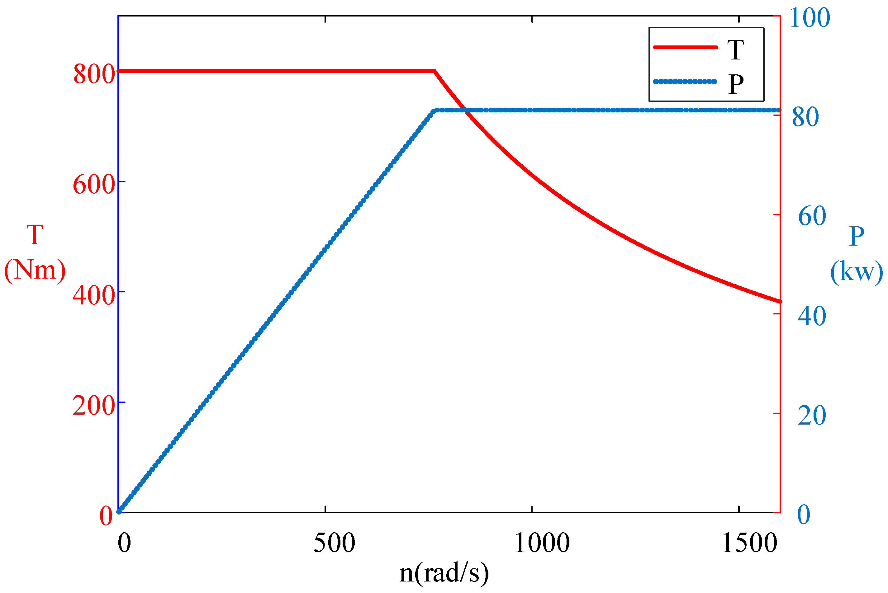
2.4. In-Wheel Motor Model

The parameters of the In-Wheel motor used in this paper are shown in

Table 2. In-Wheel motor parameters.

Description	Symbol	Value
Rated power of the motor	$P_d$	64 $\mathrm{K}\mathrm{W}$
Maximum power of motor	$P_m$	81 KW
Rated torque of motor	$T_d$	500 Nm
Maximum torque of motor	$T_m$	800 Nm
Rated speed of motor	$n_d$	800 r/min
Maximum speed of motor	$n_m$	1600 r/min

.

The power, torque, and speed of the motor are functionally related as follows, and the external characteristic curve is shown in Figure 3.

$$T=\left\{\begin{array}{cc}{T}_{\mathrm{m}\mathrm{a}\mathrm{x}}& 0⩽n⩽n_d\hfill \\ 9550\frac{P_{\mathrm{m}\mathrm{a}\mathrm{x}}}{n}& n_d⩽n⩽n_{\mathrm{m}\mathrm{a}\mathrm{x}}\hfill \end{array}\right.$$

(8)

where $T_{max}$ is the Maximum torque of the motor, $P_{max}$ is the maximum power of the motor, $n$ is the speed of the motor, $n_d$ is Motor base speed, and $n_{max}$ is a maximum speed of the motor.

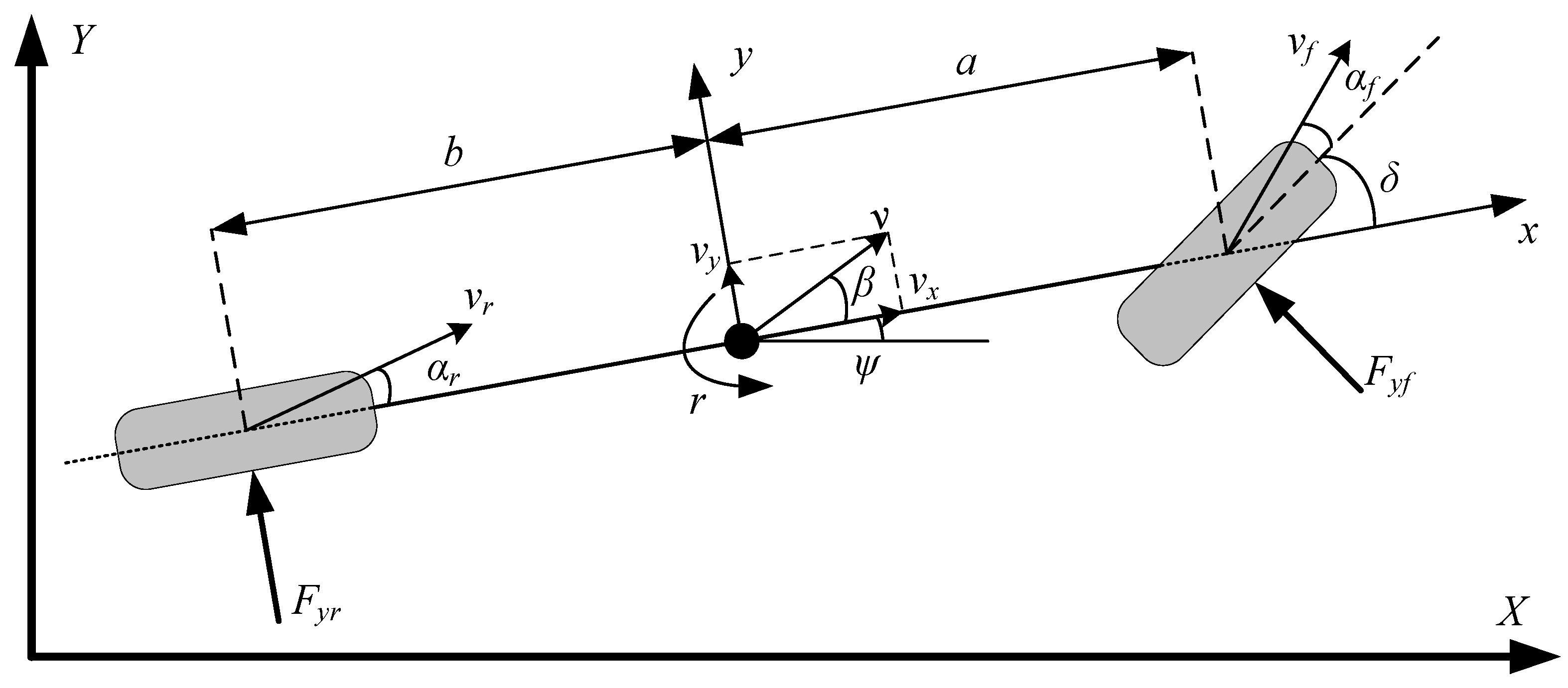
2.5. 2-DOF Vehicle Reference Model

The vehicle two-degree-of-freedom model is shown in Figure 4. Vehicle two-degree-of-freedom force analysis diagram. including lateral motion and yaw motion. Through the two-degree-of-freedom model, the ideal yaw rate and the sideslip angle of the vehicle can be calculated, and the sideslip angle, the yaw rate phase plane, can be obtained.

The dynamic equation of lateral motion and yaw motion can be expressed as follows:

$$\left\{\begin{array}{c}\dot{\beta }=\frac{k_f+k_r}{m{v}_x}\beta +\left(\frac{a{k}_f-b{k}_r}{m{v}_x^2}-1\right)\gamma -\frac{k_f}{m{v}_x}\delta \hfill \\ \dot{\gamma }=\frac{a{k}_f-b{k}_r}{I_z}\beta +\frac{a^2{k}_f+b^2{k}_r}{I_z{v}_x}\gamma -\frac{a{k}_f}{I_z}\delta \hfill \end{array}\right.$$

(9)

when the vehicle is in a stable running state, its centroid side declination angle and yaw angle speed should meet the following formula:

$$\left\{\begin{array}{c}\dot{\beta }=0\\ \dot{\gamma }=0\end{array}\right.$$

(10)

Thus, the desired yaw rate and sideslip angle can be derived as follows:

$$\left\{\begin{array}{c}{\beta }_d=\frac{b/L+ma{v}_x/\left(L^2{k}_r\right)}{1+K{v}_x^2}\cdot \delta \\ {\gamma }_d=\frac{v_x}{L\left(1+K{v}_x^2\right)}\cdot \delta \end{array}\right.$$

(11)

where $\delta$ is the front wheel angle, $L$ is the wheelbase, $K$ is the coefficient of stability, $K=\frac{m}{L^2}\left(\frac{a}{k_r}-\frac{b}{k_f}\right),k_f,k_r$ are the lateral stiffness of the front and rear wheels.

Due to the limitations of ground adhesion, the desired yaw rate needs to meet the following:

$$\left|{\gamma }_{d\mathrm{m}\mathrm{a}\mathrm{x}}\right|=\alpha \frac{\mu g}{v_x}$$

(12)

where $\alpha$ is the safety factor ($\alpha$ = 0.85), and $g$ is the acceleration of gravity ($g$ = 9.8).

The final desired yaw angular velocity is:

$${\gamma }_d=\mathrm{m}\mathrm{i}\mathrm{n}\left(\left|\frac{v_x}{L\left(1+K{v}_x^2\right)}\cdot \delta \right|,\left|{\gamma }_{d\mathrm{m}\mathrm{a}\mathrm{x}}\right|\right)sign\left(\delta \right)$$

(13)

After the sideslip angle of the center of mass is expected to be deformed:

$${\beta }_d=\frac{b/L+ma{v}_x/\left(L^{2}kr\right)}{1+K{v}_x^2}\cdot \delta =\frac{v_x^2/L}{1+K{v}_x^2}\cdot \delta \cdot \left(\frac{b}{v_x^2}+\frac{ma}{k_{f}L}\right)={\gamma }_d{v}_x\left(\frac{b}{v_x^2}+\frac{ma}{k_{f}L}\right)$$

(14)

Then it is expected that the sideslip angle of the center of mass is limited to

$$\left|{\beta }_{d\mathrm{m}\mathrm{a}\mathrm{x}}\right|=\mu g\left(\frac{b}{v_x^2}+\frac{ma}{k_{f}L}\right)$$

(15)

Therefore, the final expected sideslip angle of the center of mass is

$${\beta }_d=\mathrm{m}\mathrm{i}\mathrm{n}\left(\left|\frac{b/L+ma{v}_x/\left(L^{2}kr\right)}{1+K{v}_x^2}\cdot \delta \right|,\left|{\beta }_{d\mathrm{m}\mathrm{a}\mathrm{x}}\right|\right)sign\left(\delta \right)$$

(16)

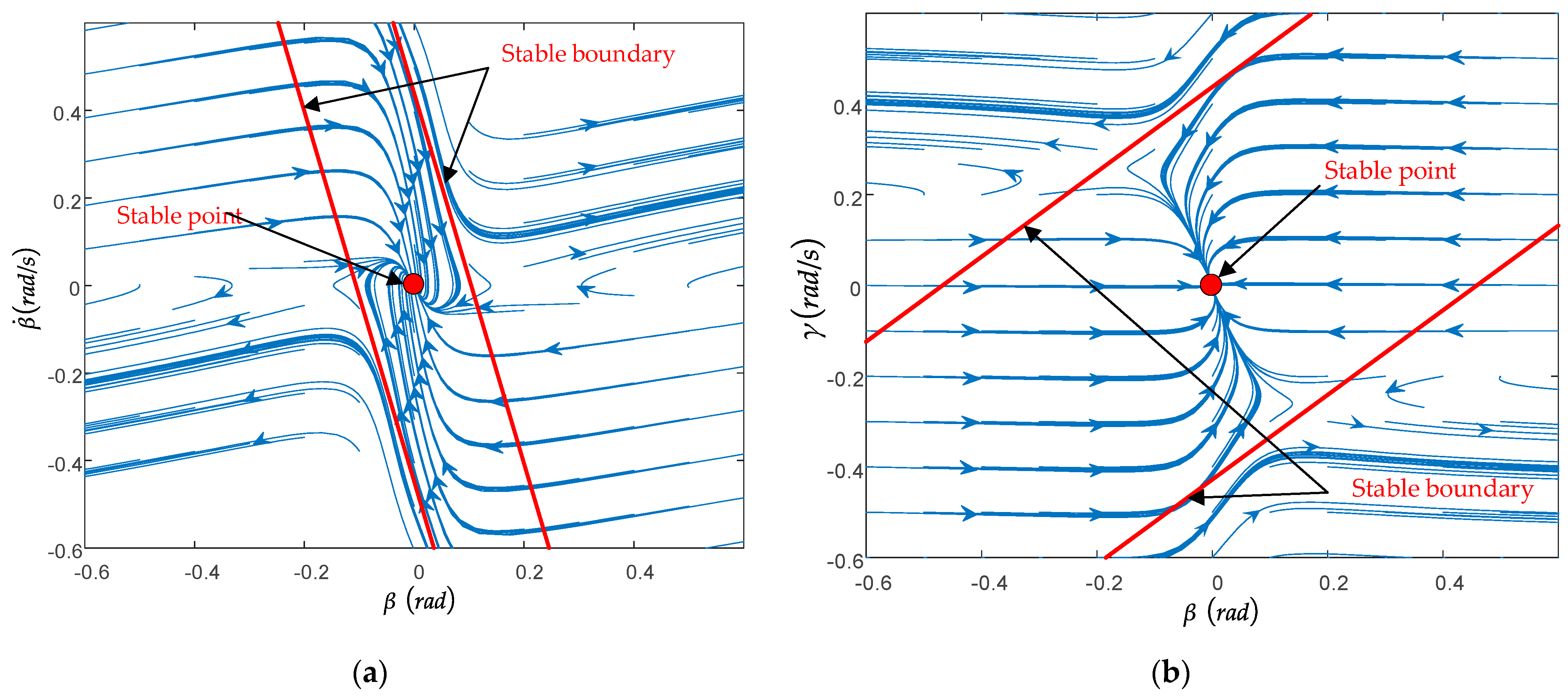
3. Establishment of Phase Plane and Stability Boundary Libraries

3.1. Establishment of Phase Plane

The phase plane analysis method is based on a two-degree-of-freedom model of the vehicle, as shown in Figure 5. The phase plane of the vehicle under different driving conditions is obtained through multiple cycles of the assignment. The phase plane mainly consists of the sideslip angle–sideslip angular velocity phase plane ($\beta -\dot{\beta }$) and sideslip angle–Yaw rate phase plane ($\beta -\gamma$).

The differential equation for the system in continuous time is:

$$\left\{\begin{array}{c}\dot{x}=f_1\left(x,y\right)\\ \dot{y}=f_2\left(x,y\right)\end{array}\right.$$

(17)

From Equation (17), we can obtain the following:

$$\frac{dy}{dx}=\raisebox{1ex}{$\frac{dy}{dt}$}\!\left/ \!\raisebox{-1ex}{$\frac{dx}{dt}$}\right.=\frac{f_2\left(x,y\right)}{f_1\left(x,y\right)}$$

(18)

From Equation (18), we can know that when $f_1\left(x,y\right)=0$ and $f_2\left(x,y\right)=0$ are established simultaneously, then $(x,y)$ is the stable point or saddle point of the system, when $f_1\left(x,y\right)=0$ and $f_2\left(x,y\right)=0$ are not established simultaneously. As can be seen from Equation (18), the slope of the passing point $(x,y)$ is unchanged at this time, so the phase trajectory through this point is unique.

In a continuous time domain system, state initial value, as the time tends to infinity, tends to a constant value, namely, $\underset{t\to \mathrm{\infty }}{\lim }x\left(t\right)=x_e$, then the system in the local scope gradually reaching stable state points in the system domain. In the phase plane, the phase trajectory of the stable state point will converge at the stable point, while the phase trajectory of the unstable state point will eventually diverge.

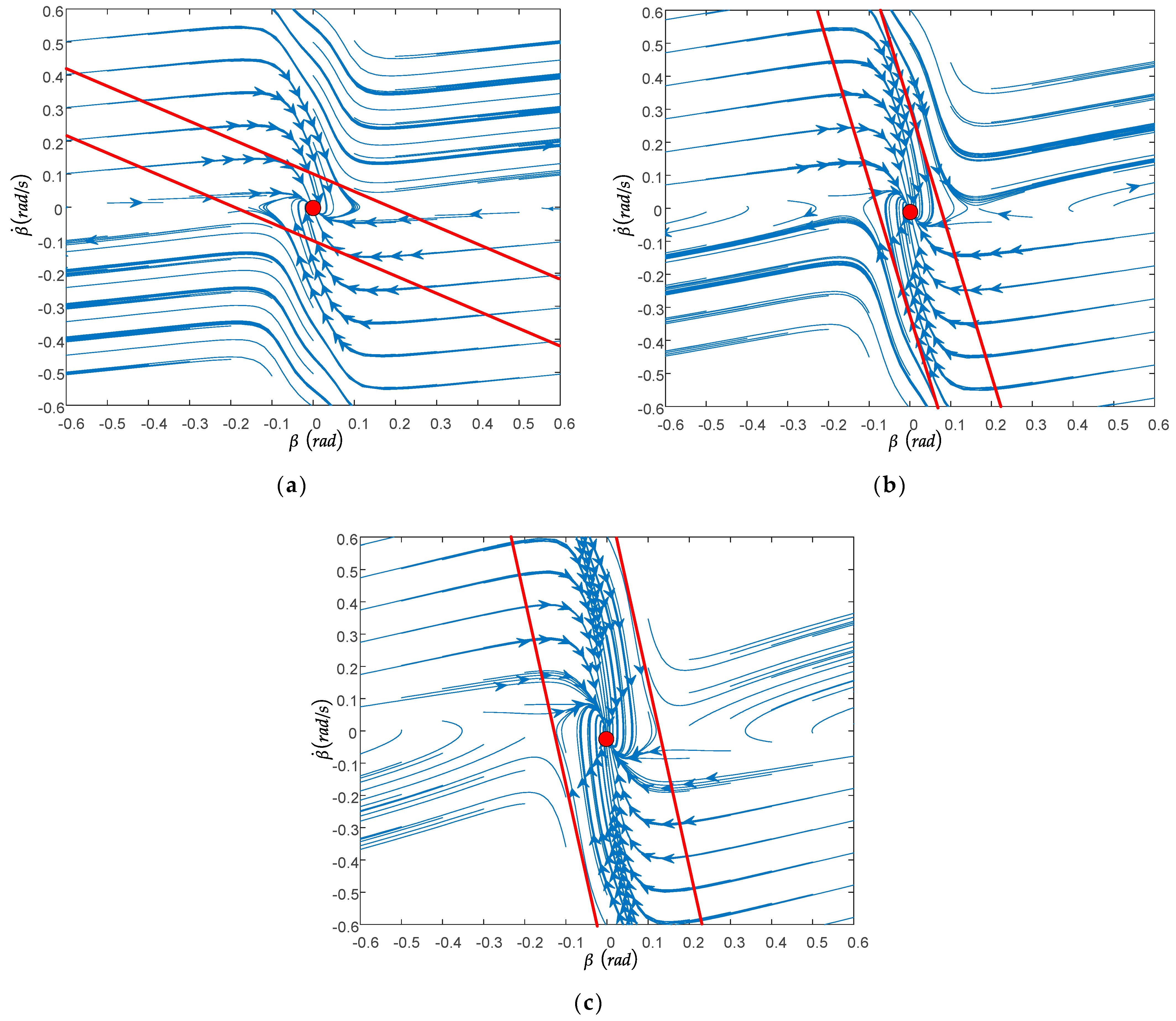
3.2. Analysis of Influencing Factors of Phase Plane Stability Region

The phase trajectory of distributed drive EV is mainly affected by longitudinal velocity, front wheel angle, and road adhesion coefficient. In this paper, the longitudinal vehicle speed is set at a fixed interval of 10 km/h, ranging from 10 km/h to 50 km/h. Turn the front wheel angle at a fixed interval of 1°, from 0° to 5°. The road adhesion coefficient is fixed at 0.1 intervals, from 0.1 to 1. According to the sample points, 300 groups of sample conditions are obtained. By analyzing the phase plane corresponding to these 300 groups of sample conditions, we can obtain the change rule of the phase plane category and the trend of phase plane change.

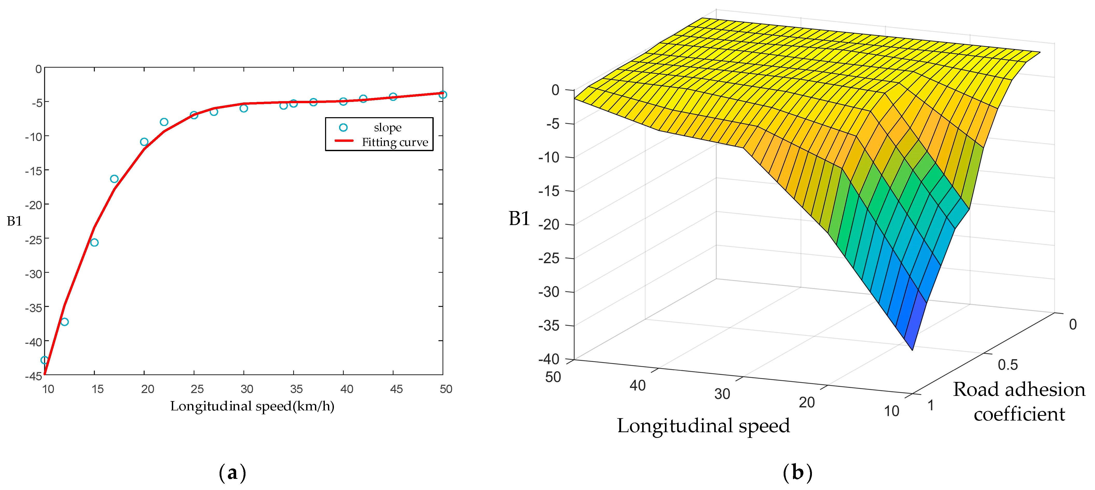
3.2.1. Influence of Longitudinal Speed on the Phase Plane

Longitudinal vehicle speeds were selected as 20, 30, and 40 km/h, respectively, and the front wheel angle was guaranteed to be 0°, and the road adhesion coefficient was unchanged at 0.8. As shown in Figure 6a–c, the trajectory of the phase tending to stability mainly distributes symmetrically according to the origin in the second and fourth quadrants, while the trajectory of the first and third quadrants mainly diverges. It can also be seen from Figure 6 that when the front wheel angle is 0°, the type of phase plane will not change.

3.2.2. The Influence of the Road Adhesion Coefficient on the Phase Plane

The road adhesion coefficients were selected as 0.3, 0.6, and 0.9, respectively; the front wheel angle was guaranteed to be 0°, and the longitudinal speed was unchanged at 40 km/h. As shown in Figure 7a–c, the trajectory of the phase tending to stability is mainly distributed symmetrically according to the origin of the second and fourth quadrants, while the trajectory of the first and third quadrants mainly diverges. With the increase in road adhesion coefficient, the slope of the stable boundary and the stable region increase gradually. Combined with Figure 7, it can also be seen that when the front wheel angle is 0, the type of phase plane will not change.

3.2.3. The Influence of the Front Wheel Angle on the Phase Plane

The front wheel angles were selected as $3^{°}$, $4^{°}$, and $5^{°}$, respectively; the road adhesion coefficient was guaranteed to be 0.5, and the longitudinal speed was constant at 50 km/h. As shown in Figure 8 the stability region of the phase plane becomes the second type of stability region, and most of the stability region is in the second quadrant. With the increase in the front wheel angle, the length BD between the intersection points of the boundary of the stability region gradually increases, but the distance AC between two points, A and C, gradually decreases, and the area of the stability region also gradually decreases.

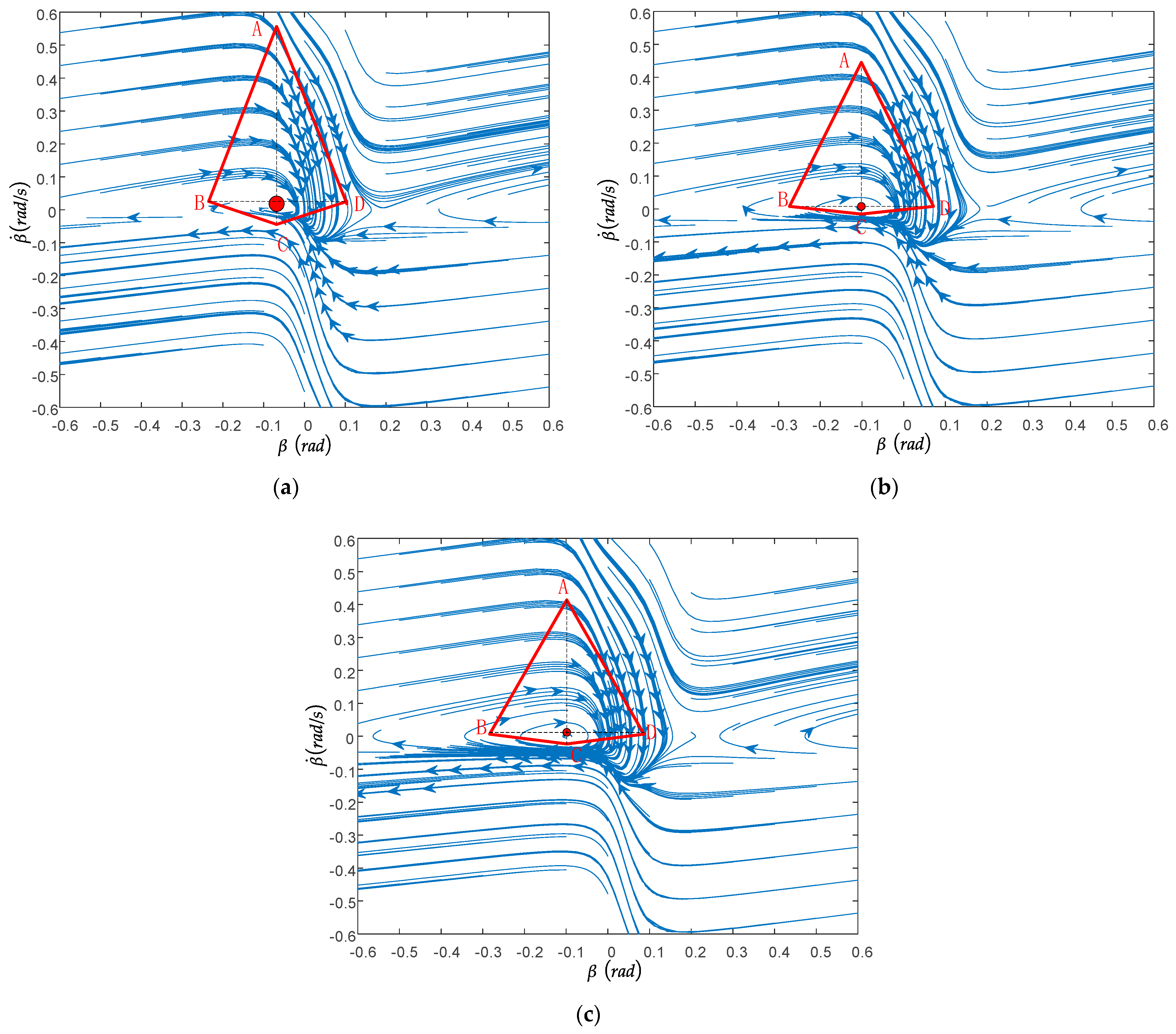
3.3. Design of Phase Plane Stability Region Boundary

3.3.1. Judgment of Boundary Type of Stable Region

According to the analysis in Section 3.2, there is a close relationship between the type of stability domain and driving conditions, including front wheel steering angle, speed, and road friction coefficient. When the front wheel angle is $0^{°}$, the phase plane category remains unchanged in the linear stability domain. When the front wheel angle changes, the phase plane category will also change. Therefore, this paper divides the phase plane into the linear stability domain and quadrilateral stability domain, as shown in Figure 9.

Before judging the stability of the current state of the vehicle, it is necessary to determine the corresponding phase plane type of the vehicle at the moment. Through the analysis of the 300 groups of data, the front wheel steering angle and vehicle speed as independent variables, and the road adhesion coefficient as a dependent variable, the three-dimensional graph was drawn. As shown in Figure 9c, when the evaluation value corresponding to the formal condition is located at the top of the three-dimensional surface, the stability domain of the vehicle corresponds to the first type, a linear stability domain. When the corresponding point is located at the bottom of the three-dimensional surface, the vehicle stability domain corresponds to the second type, the quadrilateral stability domain.

3.3.2. The Boundary Design of the First Type of Stability Region

In the linear stability domain, in order to ensure the accuracy of the design boundary in the control process and the processing of data will not be too complicated. In this paper, linear expression is adopted. As shown in Figure 9a, it can be seen that the two lines are symmetric, with the origin as the center. The right line is $L_1,$ and the left line is $L_2$. The formula is as follows, and the Coefficient table of fitting function is shown in

Table 3. Coefficient table of fitting function.

Parameter	Value	Parameter	Value
$a_1$	$5.3\times {10}^{-5}$	$a_{11}$	$-136.8$
$a_2$	$8.655\times {10}^{-3}$	$a_{12}$	$1.835\times {10}^{-3}$
$a_3$	$-0.517$	$a_{13}$	$-0.18$
$a_4$	$13.551$	$a_{14}$	$0.441$
$a_5$	$-136.802$	$a_{15}$	$149.2$
$a_6$	$-0.404$	$a_{16}$	$1.608{\times 10}^{-5}$
$a_7$	$-0.507$	$a_{17}$	$1.346{\times 10}^{-3}$
$a_8$	$-30.42$	$a_{18}$	$0.021$
$a_9$	$-0.061$	$a_{19}$	$-0.637$
$a_{10}$	$6.403$	$a_{20}$	$-64.46$

. The relationship between vehicle state and fitting coefficient is shown in Figure 10:

$$\begin{gathered} \left\{\begin{array}{c}{L}_1:\dot{\beta }=A_1\beta +B_1\\ L_2:\dot{\beta }=A_2\beta +B_2\end{array}\right. \\ \left\{\begin{array}{c}{A}_1=A_2=f\left(v\right)\\ B_1=-B_2=g\left(v,\mu \right)\end{array}\right. \\ \left\{\begin{array}{c}f\left(v\right)=a_1{v}^4+a_2{v}^3+a_3{v}^2+a_{4}v+a_5\\ g\left(v,\mu \right)=a_6+a_{7}v+a_8\mu +a_9{v}^2+a_{10}v\mu \\ +a_{11}{\mu }^2+a_{12}{v}^3+a_{13}{v}^2\mu +a_{14}v{\mu }^2\\ +a_{15}{\mu }^3+a_{16}{v}^4+a_{17}{v}^3\mu +a_{18}{v}^2{\mu }^2\\ +a_{19}v{\mu }^3+a_{20}{\mu }^4\end{array}\right. \end{gathered}$$

(19)

3.3.3. The Boundary Design of the Second Type of Stability Region

When the front wheel angle changes, the $\beta -\dot{\beta }$ phase plane type will change too. When the vehicle speed exceeds 30 km/h, and the front wheel angle exceeds $3^{°}$, the phase plane type will become quadrilateral stability domain. As shown in Figure 9b, A quadrilateral is constructed with four points of A, B, C, and D, where the horizontal coordinates of A and C are equal, and the vertical coordinates of B and D are equal. Assuming that the coordinates of point A are $({\beta }_A,{\dot{\beta }}_A)$, of point C are $({\beta }_A,{\dot{\beta }}_C)$, of point B are $({\beta }_B,{\dot{\beta }}_B)$, and of point D are $({\beta }_D,{\dot{\beta }}_B)$. Therefore, it is sufficient to determine ${\beta }_A$,${\beta }_B$,${\beta }_D$,${\dot{\beta }}_A,{\dot{\beta }}_C,{\dot{\beta }}_B$. Let the boundaries be as follows:

$$\left\{\begin{array}{c}\begin{array}{c}AB:\dot{\beta }-{\dot{\beta }}_A=\frac{{\dot{\beta }}_A-{\dot{\beta }}_B}{{\beta }_A-{\beta }_B}\left(\beta -{\beta }_A\right)\left({\beta }_B<\beta <{\beta }_A\right)\\ BC:\dot{\beta }-{\dot{\beta }}_B=\frac{{\dot{\beta }}_B-{\dot{\beta }}_C}{x_B-x_A}\left(\beta -{\beta }_B\right)\left({\beta }_B<\beta <{\beta }_A\right)\end{array}\\ \begin{array}{c}CD:\dot{\beta }-{\dot{\beta }}_{\mathrm{c}}=\frac{{\dot{\beta }}_C-{\dot{\beta }}_B}{{\beta }_A-{\beta }_D}\left(\beta -{\beta }_A\right)\left({\beta }_C<\beta <{\beta }_D\right)\\ DA:\dot{\beta }-{\dot{\beta }}_A=\frac{{\dot{\beta }}_A-{\dot{\beta }}_B}{{\beta }_A-{\beta }_D}\left(\beta -{\beta }_A\right)\left({\beta }_A<\beta <{\beta }_D\right)\end{array}\end{array}\right.$$

(20)

When the longitudinal speed remains constant, the trend of ${\beta }_A,{\beta }_D,{\dot{\beta }}_C,{\dot{\beta }}_B$ is not significant. However, the value of ${\dot{\beta }}_A$,${\beta }_B$ change significantly as the front wheel angle and road adhesion coefficient change. So, design the function $f_i\left(v\right)$ to represent ${\beta }_A,{\beta }_D,{\dot{\beta }}_C,{\dot{\beta }}_B$. Design $f_i(\delta ,\mu )$ to represent ${\dot{\beta }}_A$,${\beta }_B$, where $x_A,x_D,y_C,y_B$ are related as a function of longitudinal vehicle speed as follows. The relationship between vehicle longitudinal and Coordinate point is shown in Figure 11:

$$\left\{\begin{array}{c}{\beta }_A=f_1\left(v\right)=1.05\times 10^{-6}{v}^3+7.12\times 10^{-5}{v}^2-0.018v+0.469\hfill \\ {\beta }_D=f_2\left(v\right)=7.157\times 10^{-4}{v}^2-0.072v+1.81\hfill \\ {\dot{\beta }}_B=f_3\left(v\right)=1.039\times 10^{-5}{v}^3-1.396\times 10^{-3}{v}^2+0.06v-0.93\hfill \\ {\dot{\beta }}_C=f_4\left(v\right)=-3.02\times 10^{-6}{v}^3+0.436\times 10^{-4}{v}^2-0.022v+0.35\hfill \end{array}\right.$$

(21)

where ${\dot{\beta }}_A$,${\beta }_B$ are shown as a function of the angle of rotation of the front wheels and the coefficient of road adhesion as follows:

$$\begin{gathered} {\dot{\beta }}_A=f_5\left(\delta ,\mu \right)=0.342-0.166\delta +0.684\mu +0.017{\delta }^2-0.059\delta \mu +0.904{\mu }^2 \\ {\beta }_B=f_6\left(\delta ,\mu \right)=-0.94+0.207\delta -0.387\mu -0.016{\delta }^2-0.06\delta \mu +0.189{\mu }^2 \end{gathered}$$

(22)

4. Lateral Stability Controller Design

The front-wheel active steering system (AFS) and the direct yaw moment control system (DYC) are mainly used for vehicle yaw stability control strategies. The AFS uses the lateral force of the tires to generate additional yaw moments, and the system control function fails when the lateral force of the tires is saturated [33,34,35]. Therefore, in this paper, we use DYC to control the stability of the vehicle by using additional transverse moments.

The distributed drive electric vehicle lateral stability controller in this paper uses a hierarchical direct yaw moment control method. First, in order to obtain the optimal additional transverse sway moment, the upper layer controller uses the SMC control algorithm. The additional transverse moment is obtained by tracking the vehicle sideslip angle error. Then, the lower controller uses the optimal distribution algorithm to distribute the torque of the four wheels with the objective of optimal tire slip rate. The control framework is shown in Figure 12. The control framework.

4.1. Upper Controller Design

In this paper, the sideslip angle is selected to participate in the design of the sliding mode controller. Due to the addition of an additional yaw moment in the control process, the original two-degree-of-freedom model differential equation can be rewritten as follows:

$$\left\{\begin{array}{c}\dot{\beta }=\frac{\mathrm{c}\mathrm{o}\mathrm{s}\beta \left[\left(F_{y1}+F_{y2}\right)\mathrm{c}\mathrm{o}\mathrm{s}\delta +F_{y3}+F_{y4}\right]}{mv}-\gamma \\ \dot{\gamma }=\frac{\left[a\left(F_{y1}+F_{y2}\right)\mathrm{c}\mathrm{o}\mathrm{s}\delta -b\left(F_{y3}+F_{y4}\right)\right]}{I_z}+\frac{\Delta M_z}{I_z}\end{array}\right.$$

(23)

Here ${\Delta M}_z$ is the additional yaw moment.

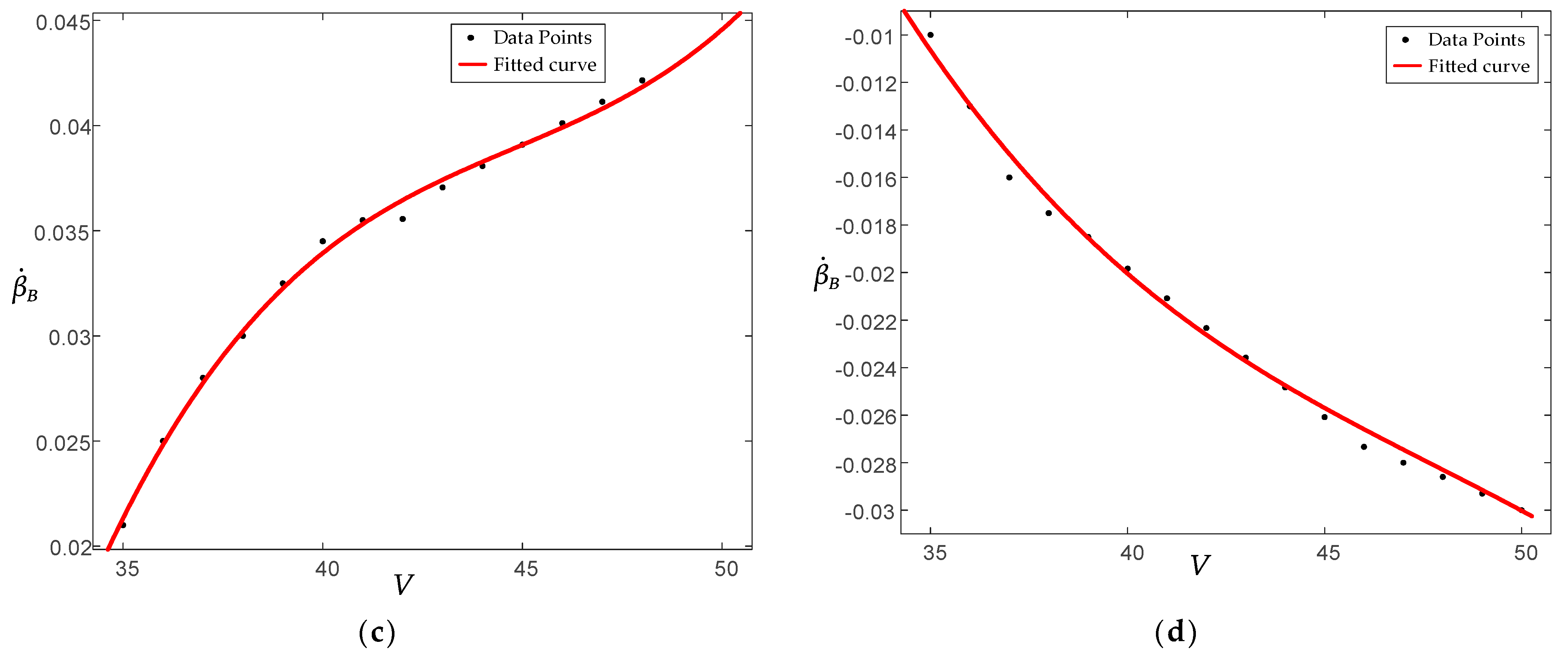
4.1.1. Yaw Moment Calculation Based on Sideslip Angle Error

The tracking error of the vehicle sideslip angle and its derivative are defined as follows:

$$\begin{gathered} e_{\beta }=\beta -{\beta }_d \\ {\dot{e}}_{\beta }=\dot{\beta }-{\dot{\beta }}_d \end{gathered}$$

(24)

On this basis, the time derivative of sliding mode surface ${\mathrm{s}}_{\beta }$ can be defined as follows:

$$s_{\beta }=c_{\beta }{e}_{\beta }+{\dot{e}}_{\beta }$$

(25)

where $c_{\beta }$ is the relative weight coefficient between the error and the rate of error change, and its value is greater than 0.

The sliding mode approach mode selects the isokinetic approach law can be defined as follows:

$${\dot{s}}_{\beta }=K_{\beta }\mathrm{s}gn\left(s_{\beta }\right)$$

(26)

where $K_{\beta }$ is the control convergence velocity to the sliding mode surface and is a positive constant.

Then:

$$\begin{array}{cc}{\dot{s}}_{\beta }& =c_{\beta }{\dot{e}}_{\beta }+{\ddot{e}}_{\beta }=c_{\beta }\left(\dot{\beta }-{\dot{\beta }}_d\right)+\left(\ddot{\beta }-{\ddot{\beta }}_d\right)\hfill \\ & =c_{\beta }{\dot{e}}_{\beta }+\frac{k_f+k_r}{m{v}_x}\dot{\beta }+\left(\frac{a{k}_f-b{k}_r}{m{v}_x^2}-1\right)\left(\begin{array}{c}\frac{a{k}_f-b{k}_r}{I_z}\beta +\frac{a^2{k}_f+b^2{k}_r}{I_z{v}_x}\gamma \\ -\frac{a{k}_f}{I_z}\delta +\frac{\Delta M_z}{I_z}\end{array}\right)-\frac{k_f}{m{v}_x}\dot{\delta }-{\ddot{\beta }}_d\hfill \end{array}$$

(27)

The additional yaw moment obtained by tracking the sideslip angle error can be defined as follows:

$$\Delta M_{\beta }=-I_z\left(\begin{array}{c}\frac{a{k}_f-b{k}_r}{I_z}\beta +\frac{a^2{k}_f+b^2{k}_r}{I_z{v}_x}\gamma -\frac{a{k}_f}{I_z}\delta \\ +\frac{K_{\beta }sgn\left(s_{\beta }\right)-{\ddot{\beta }}_d+c_{\beta }{\dot{e}}_{\beta }+\frac{k_f+k_r}{m{v}_x}\dot{\beta }-\frac{k_f}{m{v}_x}\dot{\delta }}{\frac{a{k}_f-b{k}_r}{m{v}_x^2}-1}\end{array}\right)$$

(28)

4.1.2. Controller Stability Verification

When the system state is outside the boundary layer, the control rate and switching logic remain unchanged, but if it is inside the boundary layer, the symbolic function is replaced by the saturation function $sat\left(s\right)$.

$$sat\left(s/H\right)=\left\{\begin{array}{c}sgn\left(s\right),\left|s\right|>H\\ k_{\beta }s,k_{\beta }=1/H,\left|s\right|<H\end{array}\right.$$

(29)

where $H$ is the boundary layer thickness.

In order to reduce the chattering phenomenon of the control system, the function $sgn\left(s\right)$ is replaced by the function $sat\left(s\right)$ in this paper, so the calculated yaw moment is expressed as follows:

$$\Delta M_{\beta }=-I_z\left(\begin{array}{c}\frac{a{k}_f-b{k}_r}{I_z}\beta +\frac{a^2{k}_f+b^2{k}_r}{I_z{v}_x}\gamma -\frac{a{k}_f}{I_z}\delta +\\ \frac{K_{\beta }sat\left(s_{\beta }\right)-{\ddot{\beta }}_d+c_{\beta }{\dot{e}}_{\beta }+\frac{k_f+k_r}{m{v}_x}\dot{\beta }-\frac{k_f}{m{v}_x}\dot{\delta }}{\frac{a{k}_f-b{k}_r}{m{v}_x^2}-1}\end{array}\right)$$

(30)

Define the Lyapunov function is as follows:

$$L=\frac{s^2}{2}$$

(31)

The first derivative is as follows:

$$\dot{L}=s_{\beta }\cdot {\dot{s}}_{\beta }=s_{\beta }\left(c_{\beta }{\dot{e}}_{\beta }+\frac{k_f+k_r}{m{v}_x}\dot{\beta }+\left(\frac{a{k}_f-b{k}_r}{m{v}_x^2}-1\right)\left(\begin{array}{c}\frac{a{k}_f-b{k}_r}{I_z}\beta +\frac{a^2{k}_f+b^2{k}_r}{I_z{v}_x}\gamma \\ -\frac{a{k}_f}{I_z}\delta +\frac{\Delta M_z}{I_z}\end{array}\right)-\frac{k_f}{m{v}_x}\dot{\delta }-{\ddot{\beta }}_d\right)$$

(32)

Substituting ${\Delta M}_{\beta }$ into the above formula, we can obtain the following:

$$\dot{L}=s_{\beta }\left(-K_{\beta }sat\left(s_{\beta }\right)\right)=\left\{\begin{array}{c}-K_{\beta }\left|s_{\beta }\right|,\left|s_{\beta }\right|>H\\ -K_{\beta }{k}_{\beta }{s}_{\beta }^2,\left|s_{\beta }\right|⩽H\end{array}\right.$$

(33)

Because of $K_{\beta }>0,k_{\beta }>0$, then $\dot{L}\le 0$, so the system is stable.

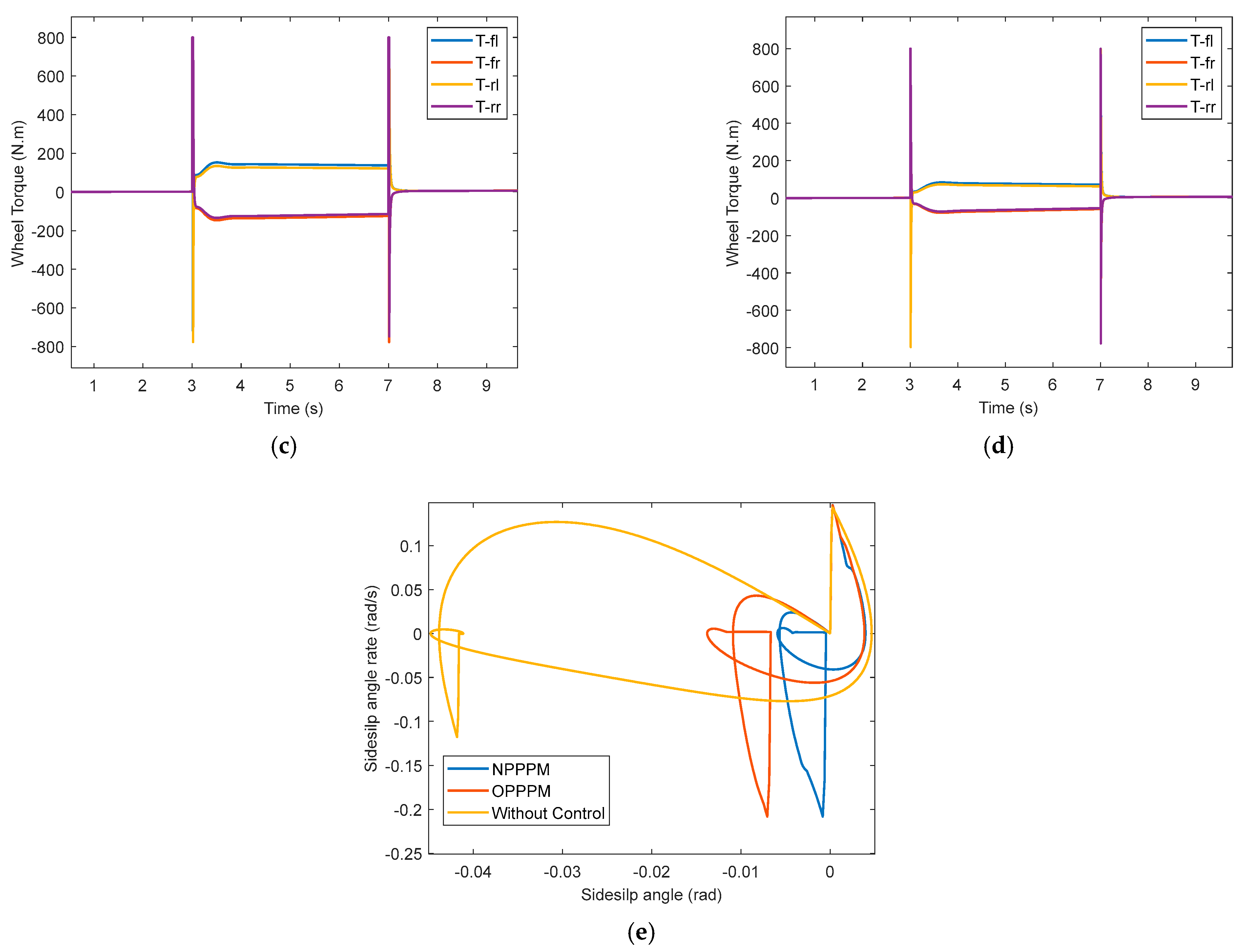
4.2. Lower Controller Design

In the previous paper, the sideslip angle is selected as the control variable, and the SMC algorithm is applied to control it so as to follow the ideal sideslip angle and solve for the additional yaw moment $\Delta M$ that can keep the vehicle laterally stable. The task of the lower controller is to distribute the solved $\Delta M$ to the four-wheel hub motors according to a reasonable algorithm in order to ensure the lateral stability of the vehicle.

In this paper, the torque optimal allocation algorithm is used, considering the tire road optimal adhesion utilization as the objective function. The road surface adhesion utilization rate can be used to describe the stability margin of the vehicle. When the road surface adhesion utilization is higher, it means that the distance between the tire force and the adhesion limit is smaller at this time, and the stability is lower. In the distributed drive electric vehicle, all four wheels can generate driving force, so the adhesion utilization rate of all four wheels needs to be considered. Therefore, the objective function used in this paper, which considers the optimal adhesion utilization of the tire road, is as follows:

$$\mathrm{m}\mathrm{i}\mathrm{n}J=\mathrm{m}\mathrm{i}\mathrm{n}\sum \frac{T_{ij}^2}{{\left({\mu }_{ij}{F}_{zij}\right)}^2}$$

(34)

In the optimization process, the objective needs to be achieved by satisfying the equation constraint requirements as the upper force and torque requirements, i.e., satisfying the cross-swing torque and the whole vehicle longitudinal force requirements, while being limited by the road attachment and motor performance. The inequality constraint requirements are the torque constraint as well as the adhesion constraint. The torque constraint is influenced by the maximum driving torque and $T_{max}$, and the adhesion constraint is mainly influenced by the tire droop load and the ground adhesion coefficient.

According to the above analysis, the constraint function can be written as follows:

$$\left\{\begin{array}{c}\begin{array}{c}{T}_{fl}+T_{fr}+T_{rl}+T_{rr}=\Delta T\hfill \\ \frac{B_f}{2r}\left(T_{fr}-T_{fl}\right)+\frac{B_r}{2r}\left(T_{rr}-T_{rl}\right)=\Delta M_{\beta }\hfill \end{array}\\ \left|T_{ij}\right|<\min \left|\left({\mu }_{ij}{F}_{zij},T_{\mathrm{m}\mathrm{a}\mathrm{x}}/r\right)\right|\hfill \end{array}\right.$$

(35)

The solution is as follows:

$$\left\{\begin{array}{c}{T}_{fl}=\frac{T}{2}-\frac{\Delta M_{\beta }}{B}r-T_{rl}\hfill \\ T_{fr}=\frac{T}{2}+\frac{\Delta M_{\beta }}{B}r-T_{rr}\hfill \\ T_{rl}=\frac{\frac{{\left({\mu }_{rl}{F}_{zrl}\right)}^2\Delta T}{2}-\frac{{\left({\mu }_{rl}{F}_{zrl}\right)}^2\Delta M_{\beta }}{B}r}{{\left({\mu }_{rl}{F}_{zrl}\right)}^2+{\left({\mu }_{fl}{F}_{zfl}\right)}^2}\hfill \\ T_{rr}=\frac{\frac{{\left({\mu }_{rr}{F}_{zrr}\right)}^2\Delta T}{2}+\frac{{\left({\mu }_{rr}{F}_{zrr}\right)}^2\Delta M_{\beta }}{B}r}{{\left({\mu }_{rr}{F}_{zrr}\right)}^2+{\left({\mu }_{fr}{F}_{zfr}\right)}^2}\hfill \end{array}\right.$$

(36)

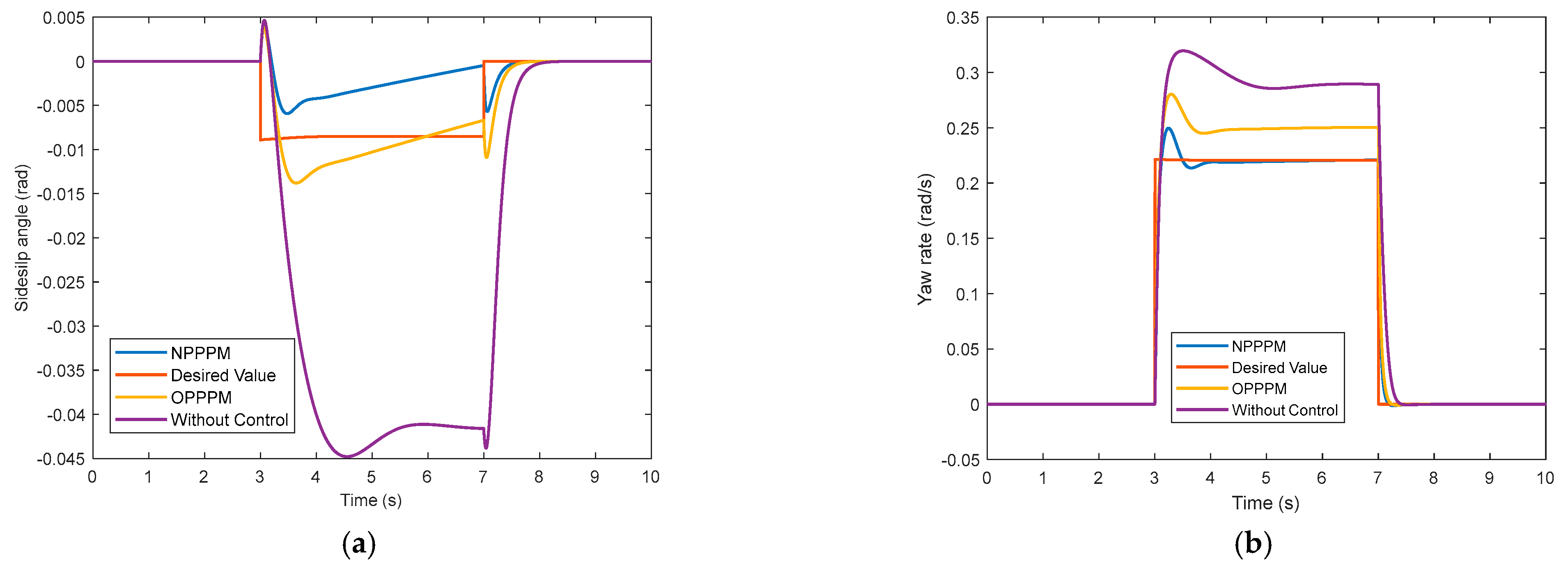
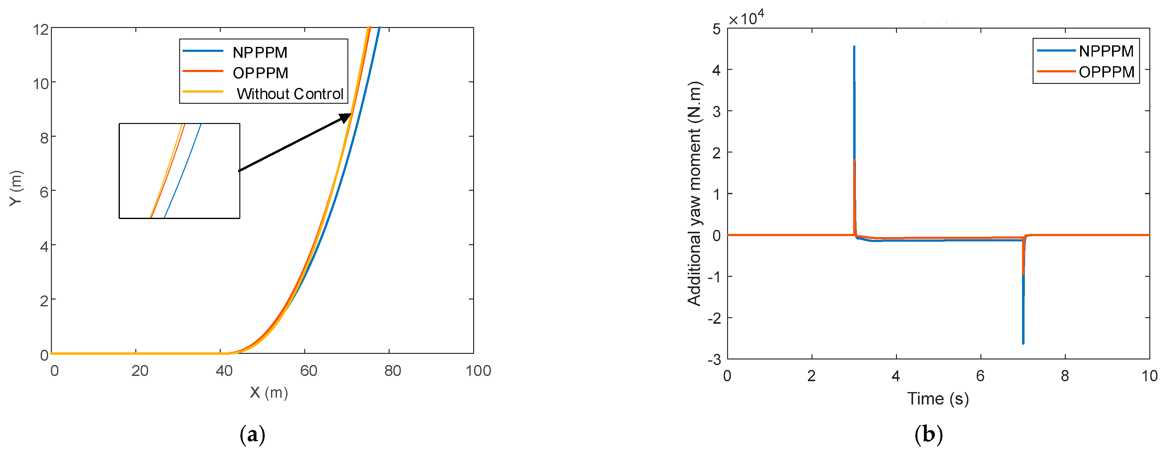
5. Simulation Verification

In order to verify the effectiveness of the distributed drive electric vehicle direct transverse moment control system under the phase plane analysis method based on the front wheel rotation angle proposed in this paper. This section conducts Matlab/Simulink-based simulation to verify it. In this paper, a new phase plane partition method (NPPPM) for phase plane stability domain partitioning and a new stability boundary expression proposed considering the effect of front wheel rotation angle on the phase plane stability boundary are presented. In this section, the proposed NPPPM is compared with the old phase plane partition method (OPPPM) and verified under DYC control at the same time.

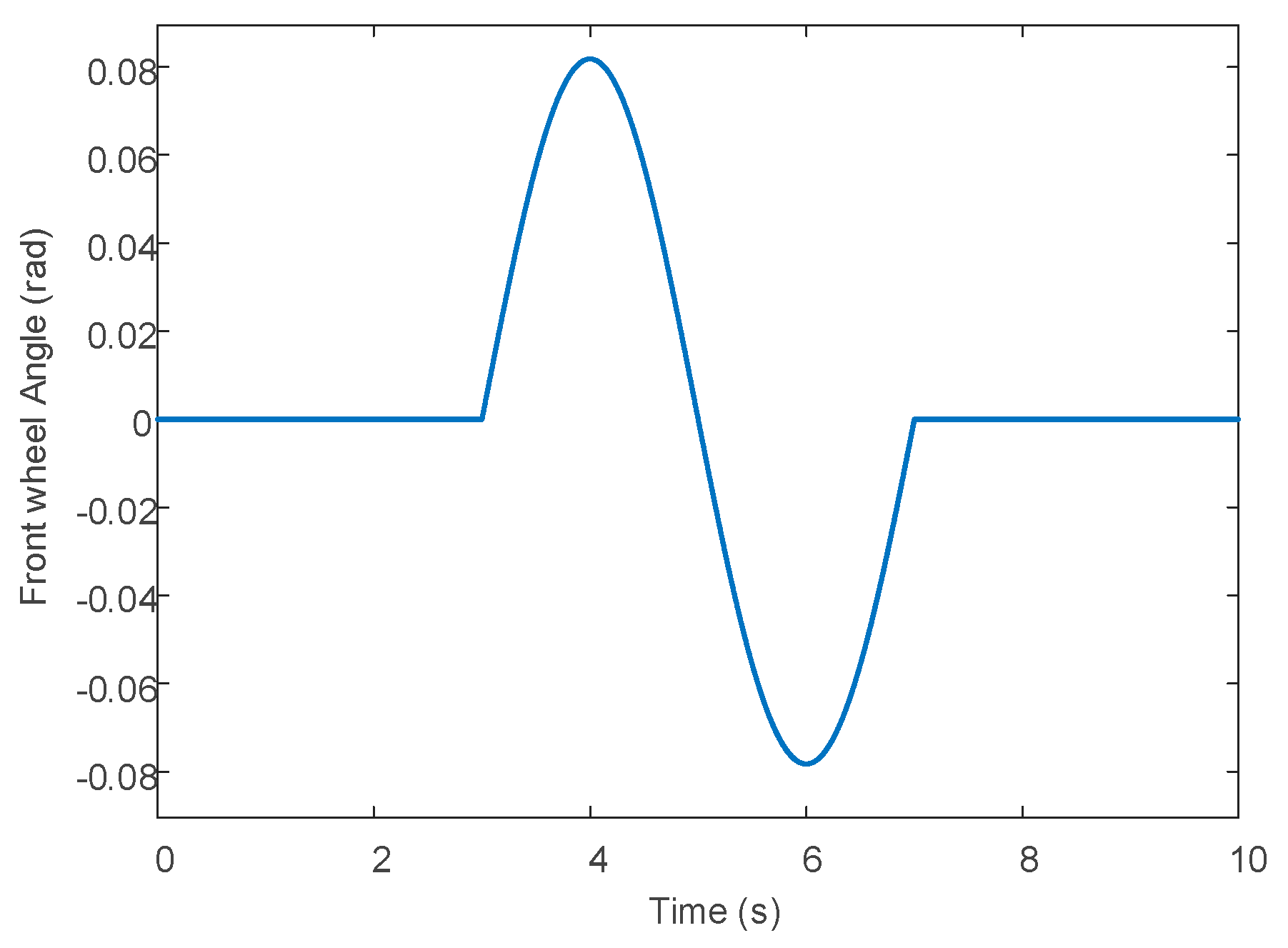
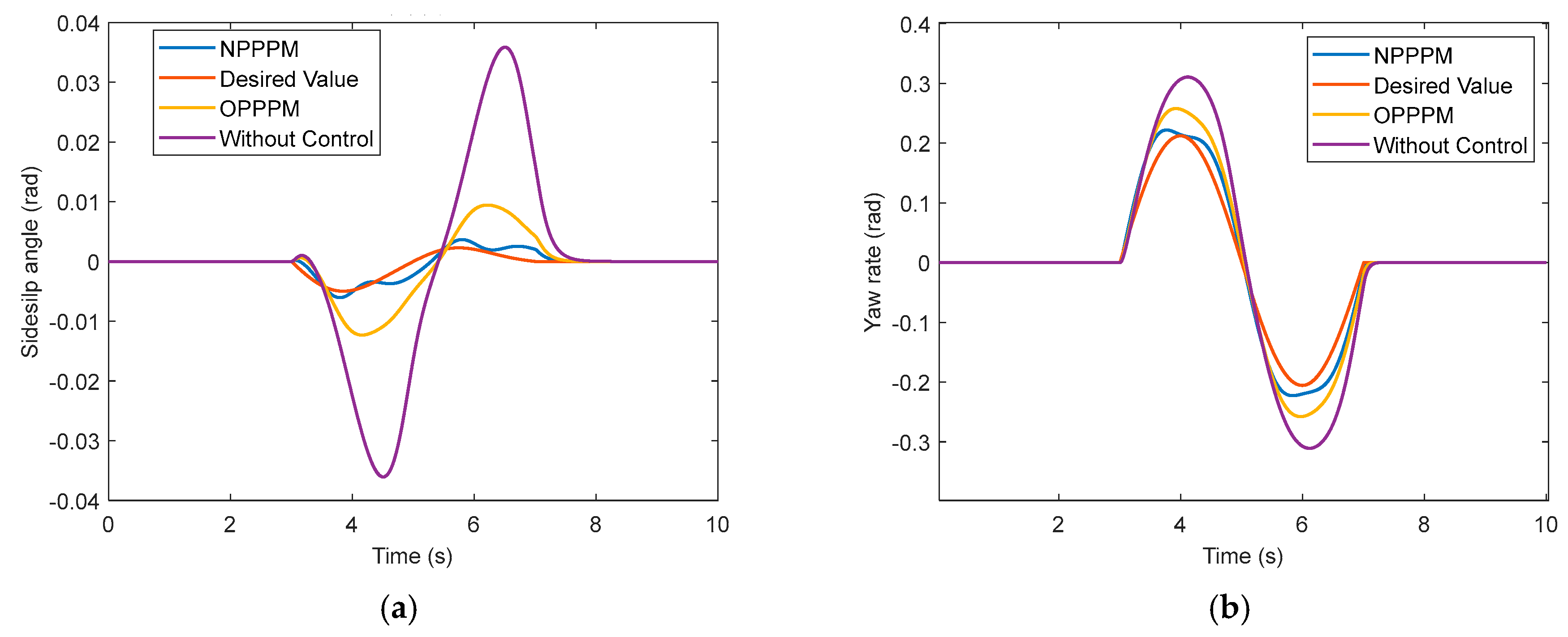
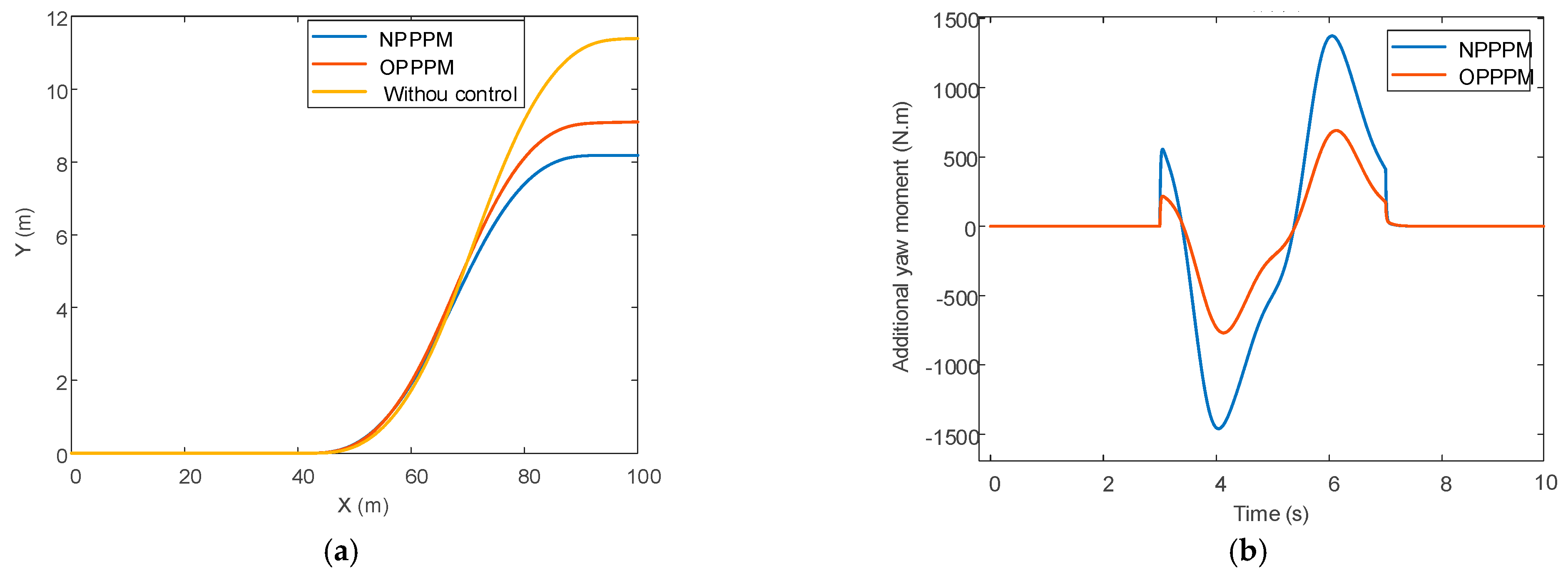
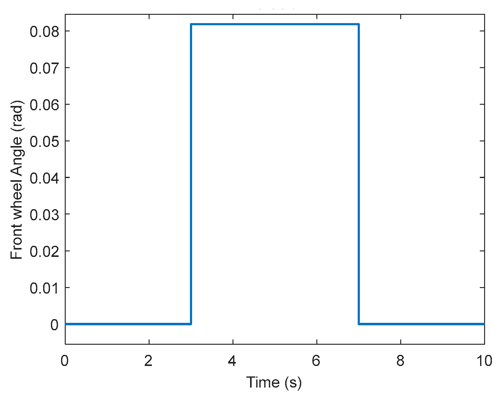
5.1. Sine Input of the Front Wheel Angle

Set the front wheel angle as a sine input with an amplitude of 0.08 rad, as shown in Figure 13 The friction coefficient of the road surface is set at 0.4 to simulate the wet road surface. Longitudinal speed is set at 50 km/h.

As can be seen from Figure 14, the wheel turning angle changes at 3 s. Before that, the vehicle keeps driving straight, and both the sideslip angle and the yaw rate can follow the ideal value. After 3 s, the actual state of the vehicle starts to deviate from the ideal value. The controller with NPPPM responded immediately after 3 s, indicating that the state of the vehicle was outside the stability domain of that phase plane at that time, the vehicle handling performance deteriorated, and the control system intervened, while the controller with OPPPM started to control only after about 3.3 s. It can be inferred that NPPPM can control the vehicle faster when the front wheel angle is changed. Moreover, we can see from the graph that the amplitude of the sideslip angle and yaw rate are 0.0079 (rad) and 0.0307 (rad/s) lower compared with those of the OPPPM method. In the maneuvering stability control system, the magnitude of the sideslip angle should be limited as much as possible to facilitate the stability control of the vehicle.

Figure 15 shows the simulation comparison of NPPPM and OPPPM under the same working conditions. As can be seen from Figure 15a, the improved phase–plane division method has better lateral control performance than the control strategy without considering the front wheel angle. Figure 15b shows the comparison of additional yaw moment based on the sideslip angle under the two division methods. The additional yaw moment under the NPPPM control method is higher than that under the OPPPM control method. The greater the additional yaw torque is applied, which ensures the lateral stability of the vehicle under the ultimate working conditions but reduces the driver’s comfort to a certain extent. Under the NPPPM control method, the torque distribution trend of the same side wheel is the same, but the amplitude is different. Front-wheel torque is greater than rear-wheel torque because the vehicle has front-wheel steering.

5.2. Step Input of the Front Wheel Angle

Set the front wheel angle as a step input with an amplitude of 0.08 rad, as shown in Figure 16. The friction coefficient of the road surface is set at 0.4 to simulate the wet road surface. Longitudinal speed is set at 50 km/h.

At this time, the sideslip angle and yaw rate curve of the distributed drive electric vehicle are shown in Figure 17. As can be seen from the figure, the peak value of the sideslip angle and yaw rate curve of the controlled centroid is lower than that of the uncontrolled one, and the curve is more stable. At the same time, it can be seen that NPPPM, which takes into account the influence of the front wheel angle on the phase plane stable boundary, has a better control effect than OPPPM under the same conditions.

Figure 18 shows the simulation comparison of NPPPM and OPPPM under the same working conditions. Figure 18a shows that the lateral displacement of the trajectory based on the NPPPM control method is small, so the lateral control of the vehicle is slightly better than the OPPPM control method. Figure 18b shows the comparison of the additional yaw moment based on the lateral yaw angle error of the center of mass under the two division methods. The additional yaw moment under the NPPPM control method is higher than that under the OPPPM control method, which leaves less operating space for the driver and reduces the driver’s handling comfort to a certain extent but ensures the lateral stability performance of the vehicle under extreme working conditions. Under the NPPPM control method, the torque distribution trend of the same side wheel is the same, but the amplitude is different. Front-wheel torque is greater than rear-wheel torque because the vehicle is front-wheel steering. The phase trajectory based on the NPPPM control method can be closed, and the phase plane is closer to the origin than that under the OPPPM control method, and the area is smaller, which well reflects the superiority of this control method.

6. Conclusions

The innovation of this paper is to propose a new method to divide and represent the phase plane stability region and establish a new phase plane stability region library based on this method. The stability boundary is designed by taking longitudinal vehicle speed, road adhesion coefficient, and front wheel angle as influencing factors. In the process of fitting the stable boundary, the least square method is used to fit 300 groups of stable points. Then, the designed phase plane stability domain library is substituted into the direct yaw moment control of the vehicle to determine the stability of the vehicle. In DYC control, a hierarchical control method is adopted. The upper layer is sliding-mode control, and the error of the centroid side deflection angle is the tracking target. The lower controller is the optimal allocation and takes the optimal road adhesion utilization rate as the objective function.

The NPPPM, OPPPM, and no control conditions with sine input and step input of the front wheel angle are compared. The simulation results show that compared with OPPPM, NPPPM has better stability judgment ability, reduces the stability range of the vehicle, improves the stability performance of the vehicle, and the four-wheel torque distribution is reasonable. Although the control comfort of the driver is reduced to a certain extent, the lateral stability of the vehicle is improved to ensure the safety of the vehicle.

References

1. Jiang, W.; Zhang, L. A Review on Stability Control Technology of Distributed Drive Electric Vehicle. Automob. Appl. Technol. 2021, 46, 210–211, 217. [Google Scholar]
2. Chen, G. A review of stability control for distributed drive electric vehicles. China-Arab. States Sci. Technol. 2021, 32, 64–66. [Google Scholar]
3. Huang, Y.; Guo, G. A Review of Torque Distribution Strategies for Distributed Drive Electric Vehicles. Automob. Appl. Technol. 2020, 45, 230–236, 248. [Google Scholar]
4. Yan, S.; Zhang, H.; Li, Q.; Gao, C. Stability Research of Four-wheel-driven Electric Vehicle Based on Co-Simulink of CarSim/Simulink. Agric. Equip. Veh. Eng. 2020, 58, 16–21. [Google Scholar]
5. Li, Y.; Xu, X. Review and Future Development of In-Wheel Motor Drive Technology. Mot. Control Appl. 2017, 44, 1–7, 18. [Google Scholar]
6. Su, L.; Zhang, F. Research Progress and Trend of Integrated Dynamics Control of Distributed Driven Electric Vehicles. Chin. J. Automot. Eng. 2022, 12, 715–733. [Google Scholar]
7. Wu, J.; Kong, Q.; Yang, K.; Liu, Y.; Cao, D.; Li, Z. Research on the Steering Torque Control for Intelligent Vehicles Co-Driving With the Penalty Factor of Human–Machine Intervention. IEEE Trans. Syst. Man Cybern. Syst. 2023, 53, 59–70. [Google Scholar]
8. Wu, J.; Zhang, J.; Nie, B.; Liu, Y.; He, X. Adaptive Control of PMSM Servo System for Steering-by-Wire System with Disturbances Observation. IEEE Trans. Transp. Electrif. 2022, 8, 2015–2028. [Google Scholar] [CrossRef]
9. Li, X. Research on Instability Mechanism and Handling Stability Control of Distributed Drive Electric Vehicles under Combined Slip Condition; Jilin University: Ji Lin, China, 2020. [Google Scholar]
10. Sachs, H.K.; Singh, M. Automobile Stability—A Study of the Domain of Attraction. Veh. Syst. Dyn. 1977, 6, 169–177. [Google Scholar]
11. Inagaki, S.; Kushiro, I.; Yamamoto, M. Analysis on Vehicle Stability in Critical Cornering Using Phase-Plane Method. JSAE Rev. 1994, 16, 216. [Google Scholar]
12. Gao, Y. Stability Control Study Based on the Stability Boundary of Phase Plane for Light Vehicle; Jilin University: Ji Lin, China, 2013. [Google Scholar]
13. Chen, Y.; Chen, Y. Study on Vehicle Instability Mechanism Based on Lyapunov First Method and Phase Plane. Veh. Power Technol. 2021, 164, 11–14, 22. [Google Scholar]
14. Zheng, X.; Zhao, Y. Design of Path Tracking Controller Based on Lyapunov Stability Theory. Automob. Technol. 2020, 539, 1–5. [Google Scholar]
15. Guo, K. Principles of Vehicle-Handling Dynamics; Science and Technology Press: Nanjing, China, 2011; p. 42. [Google Scholar]
16. Sadri, S.; Christine Qiong, W. Lateral stability analysis of on-roadvehicles using the concept of Lyapunov exponents. In Proceedings of the IEEE Intelligent Vehicles Symposium (IV), Madrid, Spain, 3–7 June 2012; pp. 450–455. [Google Scholar]
17. Sadri, S.; Christine Qiong, W. Lateral stability analysis of on-road vehicles using Lyapunov’s direct method. In Proceedings of the IEEE Intelligent Vehicles Symposium, Madrid, Spain, 3–7 June 2012; pp. 821–826. [Google Scholar]
18. Sadri, S.; Christine, W. Stability analysis of a nonlinear vehicle model in plane motion using the concept of Lyapunov exponents. Veh. Syst. Dyn. 2013, 51, 906–924. [Google Scholar]
19. Luo, Y.; Lai, E. Research on vehicle stability judgment based on energy method. Automot. Eng. 2014, 36, 1534–1538. [Google Scholar]
20. Guo, Y.; Lu, Y.; Fu, R. Simulation analysis of lateral stability of large passenger cars. China J. Highw. Transp. 2018, 31, 156–164, 230. [Google Scholar]
21. Fei, L.; Lu, X. Vehicle Stability Criterion Based on Phase Plane Method. J. South China Univ. Technol. 2014, 42, 63–70. [Google Scholar]
22. Liu, J.; Song, J.; Li, H.; Huang, H. Direct yaw-moment control of vehicles based on phase plane analysis. Proc. Inst. Mech. Eng. Part D J. Automob. Eng. 2022, 236, 2459–2474. [Google Scholar]
23. Liu, X.; Liu, J. Research on direct yaw moment control of vehicle based on phase plane method. J. Hefei Univ. Technol. 2019, 42, 1455–1461. [Google Scholar]
24. Lai, F.; Huang, C.; Ye, X. Analysis of Vehicle Driving Stability based on Longitudinal-lateral and Vertical Unified Dynamics Model. Int. J. Automot. Technol. 2022, 23, 73–87. [Google Scholar]
25. Huang, L. Study on Stability Control Strategy of 4WID Electric Vehicle Driven by Hub Moto; Hunan University: Changsha, China, 2018. [Google Scholar]
26. Zhong, L.; Peng, Y.; Jiang, M. Stability Control of Distributed Driven Electric Vehicle Based on Phase Plane. Automot. Eng. 2021, 43, 721–729, 738. [Google Scholar]
27. Xiao, F. Study on State Estimation And Direct Yaw Moment Control for In-Wheel Motor Electric Vehicles; Jilin University: Ji Lin, China, 2016. [Google Scholar]
28. Lu, M.; Xu, Z. Integrated Handling and Stability Control with AFS and DYC for 4WID–EVs via Dual Sliding Mode Control. Autom. Control Comput. Sci. 2021, 55, 243–252. [Google Scholar]
29. Gong, T.; Xie, X. A Control Strategy of Vehicle Electronic Stability Based on Phase Plane Method. J. Transp. Inf. Saf. 2019, 37, 83–90. [Google Scholar]
30. Song, Y.; Shu, H.; Chen, X. Direct-yaw-moment control of four-wheel-drive electrical vehicle based on lateral tyre–road forces and sideslip angle observer. IET Intell. Transp. Syst. 2019, 13, 303–312. [Google Scholar]
31. Wang, H.; Han, J.; Zhang, H. Lateral Stability Analysis of 4WID Electric Vehicle Based on Sliding Mode Control and Optimal Distribution Torque Strategy. Actuators 2022, 11, 244. [Google Scholar]
32. Sun, X.; Wang, Y.; Cai, Y.; Wong, P.K.; Chen, L.; Bei, S. Nonsingular Terminal Sliding Mode based Direct Yaw Moment Control for Four-Wheel Independently Actuated Autonomous Vehicle. IEEE Trans. Transp. Electrif. 2022, in press.
33. Ji, Q. Research on Yaw-Roll Stability Control of Distributed Drive Electric Vehicle; Xihua University: Cheng Du, China, 2021. [Google Scholar]
34. Lan, S. Research on Coordinated Control of Roll Stability and Braking Stability Performance of Distributed Electric Vehicle; Liaoning University of Technology: Jin Zhou, China, 2021. [Google Scholar]
35. Wang, J. Steering Stability Control of Four-Wheel Drive Vehicle with Hub Motors; Beijing Institute of Technology: Beijing, China, 2015. [Google Scholar]
Figure 1. Vehicle seven-degree-of-freedom model.
Actuators 12 00121 g001
Figure 2. Wheel models.
Actuators 12 00121 g002
Figure 3. Motor external characteristics curve.
Actuators 12 00121 g003
Figure 4. Vehicle two-degree-of-freedom force analysis diagram.
Actuators 12 00121 g004
Figure 5. The phase plane type: (a) sideslip angle–sideslip angular velocity phase plane ( β β ˙ ); (b) sideslip angle–yaw rate phase plane ( β γ ).
Actuators 12 00121 g005
Figure 6. Influence of longitudinal speed on the phase plane: (a) V x = 20   k m / h , μ = 0.8 ; (b) V x = 30   k m / h , μ = 0.8 ; (c) V x = 40   k m / h , μ = 0.8 .
Actuators 12 00121 g006
Figure 7. The influence of the road adhesion coefficient on the phase plane: (a) V x = 40   k m / h , μ = 0.3 ; (b) V x = 40   k m / h , μ = 0.6 ; (c) V x = 40   k m / h , μ = 0.9 .
Actuators 12 00121 g007
Figure 8. The influence of the front wheel angle on the phase plane: (a) V x = 50   k m / h , δ = 3 ° ; (b) V x = 50   k m / h , δ = 4 ° ; (c) V x = 50   k m / h , δ = 5 ° .
Actuators 12 00121 g008
Figure 9. Judgment of boundary type of stable region: (a) Linear stability domain; (b) Quadrilateral stability domain; (c) Trend of phase plane stability region.
Actuators 12 00121 g009
Figure 10. Boundary coefficients of the first type of stability regions as a function of driving state: (a) The fitting curve of longitudinal speed and B1; (b) The nonlinear relationship between B2 and its influencing factors.
Actuators 12 00121 g010
Figure 11. Boundary coefficients of the first type of stability regions as a function of driving state: (a) Trend of β A with longitudinal vehicle speed; (b) Trend of β D with longitudinal vehicle speed; (c) Trend of β ˙ B with longitudinal vehicle speed; (d) Trend of β ˙ C with longitudinal vehicle speed.
Actuators 12 00121 g011aActuators 12 00121 g011b
Figure 12. The control framework.
Actuators 12 00121 g012
Figure 13. Sine input of the front wheel angle.
Actuators 12 00121 g013
Figure 14. Comparison of sideslip angle and yaw rate curves under DYC control: (a) Comparison of sideslip angle; (b) Comparison of yaw rate.
Actuators 12 00121 g014
Figure 15. Simulation comparison of NPPPM and OPPPM under DYC control with sine input for front wheel angle: (a) Path comparison; (b) Additional yaw moment comparison; (c) Four-wheel torque at NPPPM; (d) Four-wheel torque at OPPPM; (e) Phase–plane contrast.
Actuators 12 00121 g015aActuators 12 00121 g015b
Figure 16. Step input of the front wheel angle.
Actuators 12 00121 g016
Figure 17. Comparison of sideslip angle and yaw rate curves under DYC control with step input of the front wheel angle: (a) Comparison of sideslip angle; (b) Comparison of yaw rate.
Actuators 12 00121 g017
Figure 18. Simulation comparison of NPPPM and OPPPM under DYC control with step input of the front wheel angle: (a) Path comparison; (b) Additional yaw moment comparison; (c) Four-wheel torque at NPPPM; (d) Four-wheel torque at OPPPM; (e) Phase–plane contrast.
Actuators 12 00121 g018aActuators 12 00121 g018b