Exploring the Dynamic Shock of Unconventional Monetary Policy Channels on Income Inequality: A Panel VAR Approach

Abstract

In response to the “Great Recession and Global Financial Crisis”, central banks had to deploy unconventional monetary policies (UMP) in order to fight the severe impact of the crisis. Therefore, the purpose of this study is to examine the dynamic shock of unconventional monetary policies through earning heterogeneity, income composition, and portfolio channels on income inequality in emerging economies covering the period 2000–2019, using the panel vector autoregressive (PVAR) model. A PVAR model was designed for this study because of its ability to address the dynamics of numerous entities considered in parallel. The findings suggest that the UMPs used by these countries’ central banks may have increased income inequality through all of the channels investigated in this study, as a shock to unconventional monetary policy results in a positive response in income inequality. Even when pre-tax income, held by the top 10%, is adopted to measure income inequality, the study yields similar results. It is evident that a central bank’s objective is and should be to fulfil its mandate of achieving maximum employment and price stability, thus bringing wide economic benefits. Thus, some forms of policies are more appropriate for addressing concerns about inequality (income policy or fiscal policy) than others. However, the current study alerts the central bank to the fact that monetary policies may have a wounding impact on income inequality. Therefore, the central banks should consider the cost of monetary policies on income inequality when drafting or implementing these kinds of policies.

1. Introduction

The outbreak of the 2007–2009 financial crisis in the United States, which ultimately spread widely across many countries, mainly driven by the interaction of the financial markets in recent decades, has caused a wide range of economic changes. In various countries, including emerging markets, output has suffered a major shock, and has not yet recovered to pre-crisis levels in many cases. The recent history shows that interest rates have been at lower levels in many countries. A dramatic escalation was observed in unemployment before improving again in some countries. In other countries, it remained unacceptably high. Since the 1980s, income and wealth inequality, measured by the income and wealth share of the top decile and the Gini coefficient, have been recorded, showing a surge in various countries (Piketty 2014; Atkinson 2014; Sarfati 2016). During the havoc caused by the crisis, central banks in various countries reduced the negative impact of the crisis by cutting interest rates at a faster pace, while in countries such as the US and Europe it got closer to 0%. However, after the bankruptcy of Lehman Brothers in September 2008, the crisis gained a global magnitude, with its effects felt in almost every segment of the market and not just real estate. The central banks were confronted with a diminished financial sector and appeared to have reached the limits of what they could accomplish with conventional tools, as financial conditions did not respond sufficiently to a reduction in policy rates. Later on, conventional policy easing ran into the constraints of the effective lower bound. This, then, emphasized the necessity for the central banks to undertake innovative policy actions in pursuit of their mandates and be consistent with their legal framework to deal with the global financial crisis and its aftermath. Against this backdrop, the central banks gradually introduced a set of policy measures that have come to be collectively known as unconventional monetary policy tools (UMP) to address the challenges posed by the crisis and the economic environment that ensued.

The main tool under conventional monetary policy was to control the short-term interest rate; changes in this policy rate and the public’s expectations of its future settings affected financial conditions (the availability and cost of funding) and, further down the transmission channel, affected the macro-economy (aggregate spending, output, and inflation). Unlike conventional policy tools, unconventional instruments target various measures rather than short-term interest rates. These tools are classified into four categories: negative interest rate policies; expanded lending operations; asset purchase programs; and forward guidance. These tools were designed for asset valuations and to restore the liquidity conditions in the financial system as a means of supporting the monetary policy transmission mechanism, while others aimed to affect term spreads (equivalently, long-term risk-free rates). Others were designed to be directed at influencing credit spreads and liquidity (or, equivalently, interest rates on various non-risk-free instruments). However, during the financial crisis the challenging part was the implementation of the UMP since its transmission mechanisms might have been affected by the disruptions.

Recently, some economists and politicians have begun to question the subsequent increase in inequality. The UMP measures implemented by several central banks around the world are among the possible causes of the noticeable increase in income inequality we see today. This concern was further raised by the former chairwoman of the Federal Reserve, Janet Yellen, in 2014, when she expressed concern about worsening inequality (Yellen 2014). Therefore, the pressing question is: who in society do these measures potentially benefit? The key problem here is that non-traditional measures would primarily benefit those at the top of the income scale, unfairly distributing the good impacts of expansionary monetary policy. Thus, these developments have become a concern as increasing inequality may reduce economic growth (OECD 2014) and contribute to financial fragility (Rajan 2010; Bordo and Meissner 2012; Kumhof et al. 2015; Zungu and Greyling 2022), or increase social conflict due to lower social mobility (Wilkinson and Pickett 2009; Corak 2013; OECD 2014). Among the studies on this subject matter, some support the argument made by economists and politicians that the UMP implemented by the central banks in fighting the financial crash of 2007 was the main determinant of the increasing wealth and income inequality in the world (Saiki and Frost 2014; Bullard 2014; Lenza and Slacalek 2019). On the other hand, others argue that it plays a significant role in easing the severe impact posed by the crisis. It also triggers policy concerns that such measures may have serious effects on economic inequalities (Casiraghi et al. 2018; Guerello 2018; Colciago et al. 2019; Lenza and Slacalek 2019), while others find inconclusive results (Colciago et al. 2019).

The distributional effects of these policy tools have been largely ignored in academic literature and in the daily lives of the central banks. However, the recent escalation of inequality highlights the importance of this issue to be kept on board by the central bank. Furthermore, in this context, and in light of the widely held belief that high-income individuals are becoming even wealthier through financial markets, it raises the question of whether the MP has skewed wealth and income distribution. As a result, the question of the role of the MP and the consequences of its transmission channels on income inequality dynamics deserve a more in-depth examination in order to properly assess the unfavourable implications of expansionary UMPs. Furthermore, the contradictory findings reported in the literature indicate that more research is needed in this area, as Bernanke (2015) and others argue that, in order to explore and quantify the full effects of monetary policy on income and wealth inequality, it is critical to identify channels through which monetary policies could have distributive effects.

This study extends the existing literature on this subject matter following the seminal work of Alves and Silva (2020), utilizing the panel corrected standard errors and the fixed effect approach in the Euro Area covering the period 1999–2017. In their model, the impact of UMP on income inequality was investigated through the income composition channel, which was captured using the equity index. Considering the argument made by Bernanke (2015), our work is distinct from that of Alves and Silva (2020) and those that are found in the literature as we aim to contribute to the existing debate on this topic by identifying and quantifying three transmission channels that are thought to be the most relevant monetary policy channels in examining the dynamic impact of UMP on income inequality, namely earning heterogeneity, income composition, and portfolio composition channels. Unlike Alves and Silva (2020), we used the Gini coefficient at market income from the Standardized World Income Inequality Database (Solt 2020) and the pre-tax income held by the top 10% (PTI10%) from the World Inequality Database (Alvaredo et al. 2018). These inequality measures are adopted in comparing the impact of UMP through the adopted channels. The study Alves and Silva (2020), focuses on the high income countries.

This study seeks to fill the gap in the literature by incorporating and examining the impact of the development of the UMP and its effects on income inequality in emerging markets, which most of the existing studies have not paid attention to, and also by providing evidence of which monetary policy channels are beneficial to income inequality among the three channels. The purpose of this study is to clarify the ongoing debate in the literature by constructing a balanced panel data set of 15 emerging markets from 2000 to 2019, using the panel vector autoregressive (PVAR) technique. The PVAR will be used to answer the following hypothesis: how income inequality responds to a shock of unconventional monetary policy. The low income groups suffer the most during the adoption of the unconventional monetary policy compared to the high income groups.

We developed a PVAR because of the variety of measured defects. This model allows us to investigate the dynamic interactions of several entities at the same time, rather than confining the research on a single object. For example, in this study, we investigate the interactions that occur between 15 countries that we adopted, as they are characterised by the same monetary policy, or trade intensively. In this instance, panel VAR models that address the dynamics of numerous entities considered in parallel, are significant for this type of study. These models are often deeper than standard VAR models since they not only examine the interaction between variables naively, as a conventional VAR model would, but they also add a cross-subsectional structure to the model. This allows us to differentiate common components from particular components, whether in terms of countries, variables, or time periods etc., and then to utilize this structural knowledge to improve the accuracy of the estimation. It becomes much more resilient when dealing with data of uncertain quality and often short duration. These features cannot be accounted for by static panel techniques, nor by interaction effects. Finally, the motivation for this study stemmed not from a lack of studies examining the impact of an UMP on income inequality in emerging countries, but rather from the fact that this relationship may differ from the one found in the literature, due to differences in the smoothness of the economic development and the macroeconomic policies implemented. Actually, the findings of the study documented that the UMPs applied by the central banks in these countries could increase income inequality through the earning heterogeneity, income composition, and portfolio channels examined in this study. This was further evident even when we adopted the pre-tax income held by the top 10% to capture income inequality.

2. Theoretical Framework

2.1. Theoretical Channels of Monetary Policy and Income and Wealth Inequality

This section focuses on the theoretical channels that link monetary policy and income and wealth inequality. From the literature, six channels have been selected to explain the relationship between monetary policy and income and wealth inequality (Colciago et al. 2019). Some believe that an accommodative monetary policy would help to achieve a more equitable income distribution, namely earning heterogeneity and saving redistribution channels, while others maintain that an accommodative monetary policy would lead to an increase in wealth and inequality, namely portfolio, income composition, and financial segmentation channels. The impact of monetary policy on income inequality depends on the structure of the asset portfolio and income of the household, where the total income of the household is derived from two sources: capital and labour. In this context, “capital income” is defined as the income earned by households from their wealth, which includes deposits, equity, property, and bonds. Labour income, on the other hand, is a function of wages and labour supply. Thus, the analysis in this study is restricted to three main channels, namely earning heterogeneity, income composition, and the portfolio composition channels, which may affect inequality dynamics differently.

Accommodative monetary policy may help in achieving a more equitable income distribution through the (i) earnings heterogeneity channel, which reflects the impact that monetary policy may have on households’ wages and employment status. Since, when the unemployment rate in lower and middle-income families is high, an expansionary UMP appears to benefit them primarily by reducing the stress of finding work, which tends to decrease income and wealth inequality (Carpenter and Rodgers 2004). This was further supported by Heathcote et al. (2010), who showed that labour earnings at the bottom of the distribution levels are most affected by business cycle fluctuations and that an expansionary monetary policy could potentially reduce income inequality. Another study by Huber and Stephens (2014) found evidence that a monetary policy-induced lowering of the unemployment by 1% could reduce the Gini coefficient for market income by approximately 0.4 points.

A second channel, is the (ii) savings redistribution channel, which is the one that is related to the differences in net financial positions among households’ balance sheets. The Central Bank (CB) reduces interest rates to below 0% levels and tries to reduce long-term interest rates using UMP measures. The assumption is that lenders are richer than borrowers. Therefore, in this scenario, an expansionary UMP that has an increasing effect on inflation or that aims to reduce interest rates will benefit the real value of the borrowers against the real value of savers (Nakajima 2015).

Another group of channels are those who argue that accommodative UMP would imply an increase in inequality and wealth income. Assuming a heterogeneous household with different sources of income, (iii) the income composition is different for each economic agent and these channels arise from the fact that the impact monetary policy may have regarding its composition. These demonstrate that the households with a higher proportion of interest income, which are normally the richest households, would benefit if an expansionary UMP shock increases assets and financial income more than wages (Galbraith 1998; Coibion et al. 2012). Looking at (iv) the portfolio composition channel, it is associated with the fact that a fall in interest rates affects the asset holdings of households. Therefore, if higher income households maintain a greater proportion of their wealth in assets, they would benefit more from an extensive UMP that increases the prices of assets (Brunnermeier et al. 2012). However, if these measures create inflation, it would adversely affect households that need more cash for their transactions. On the other hand, the study by Bhattacharya (2005) argue that the older generations own more cash and are greater consumers compared to younger generations, thus producing a transfer of income between generations. Furthermore, it was noted in the literature that the low-income segment become more affected when they regularly keep their wealth (Erosa and Ventura 2002). In this case a UMP might increase inequality due to an increase in financial assets.

The benefit received from increases in asset prices by high-income households could also occur through the (v) financial segmentation channel. Under the assumption that richer households tend to be more connected to financial markets, monetary policy-induced changes may benefit the more connected households more (Williamson 2009). For example, wealthy people typically have greater access to financial markets, giving them more opportunities to diversify their portfolios, protect themselves in times of crisis, and capitalize on opportunities.

Finally, (vi) the unexpected inflationary channel demonstrates that inflation may have an effect on household cash position and fixed debts. In this scenario, the debtors benefit more than the creditors.

2.2. Theoretical Channels of Monetary Policy and Income and Wealth Inequality

The distributional effect of monetary policy, in particular UMP, has been given little attention in the literature compared to the effect of fiscal policy. Moreover, the distributional effect has been treated as being small on macroeconomic variables. However, Mark Carney, the vice chairman and head of Impact Investing at Brookfield Asset Management, in his statement, illustrated that “all monetary policy has a distributional effect” (Carney 2016). The uncertainty surrounding the monetary policy pertains to the size and direction of its effect in different monetary policy setups, since the distributional impact of monetary policy is shared by central bankers. In this section, we will start by reviewing the empirical literature on conventional monetary policy (CMP) and income inequality, and then elaborate to include evidence on UMPs.

2.2.1. Effects of Conventional Monetary Policy on Inequality

The existing empirical literature on the distributional impact of the CMP shows that an unexpected increase in the interest rate increases income inequality. Moving as far back as the study by Romer and Romer (1999), which became the first study to investigate the impact of the CMP on poverty, their findings show that an expansionary monetary policy temporarily alleviates poverty, but only through low inflation and stable output.

Mumtaz and Theophilopoulou (2017) studied the subject matter for UK covering the period 1969 to 2012, using the SVAR model. Their finding shows that contractionary monetary policy shocks lead to an increase in earnings, income, and consumption inequality and contribute to their fluctuation. They point out policy of quantitative easing as one of the contributors to the increasing inequality during the Great Recession. Their findings were supported by Furceri et al. (2018), who studied the same subject matter in a panel of 32 advanced and emerging economies, covering the period 1990–2013. In their approach, they changed the short-term interest rates that are orthogonal to the unexpected changes in growth and inflation news. A further support to the existing studies that believe CMP is income improving was documented by El Herradi and Leroy (2019) using the data from 12 advanced economies between 1920 and 2015 and the Panel VAR approach. Contradicting results were documented by Apanisile (2021) in the case of Nigeria, where they studied the anticipated and unanticipated shock of conventional monetary policy on income inequality, using the Dynamic Stochastic General Equilibrium approach. The findings show that both anticipated and unanticipated shocks have the same effect on income inequality, namely to reduce income inequality in the country.

2.2.2. Effects of Unconventional Monetary Policy on Inequality

After scrutinizing the empirical literature on this subject, we found the distribution mechanisms of a UMP to be even less straightforward. The UMP is based on the size of the central bank’s balance sheet rather than interest rates. These kinds of policy instruments often inflate the prices of financial assets, which tend to be held by the wealthy rather than the poor, thus potentially increasing inequality. The existing literature on this subject matter is diverse. Some studies establish that the UMP is the main determinant of income and wealth inequality (Gambacorta et al. 2012; Saiki and Frost 2014; Kimura and Nakajima 2016; Davtyan 2016; Israel and Latsos 2019; Rupprecht 2020; Evgenidis and Fasianos 2021); others, a find it to have a distributional effect (Casiraghi et al. 2018; Guerello 2018; Lenza and Slacalek 2019).

Furthermore, we have discovered that the literature has created two strands indicating that UMP impacts income and wealth inequality through different channels. The first strand, formed by a group of studies, argues that accommodative UMP helps to establish a more equitable income distribution through the saving redistribution and earnings heterogeneity channels (Doepke and Schneider 2006; Heathcote et al. 2010; Bivens 2015; Casiraghi et al. 2018; Guerello 2018; Lenza and Slacalek 2019), while the second strand believes that these policies will increase income and wealth inequality via the portfolio, income-composition and financial segmentation channels (Amaral 2017; Mumtaz and Theophilopoulou 2017; Albert et al. 2019; Taghizadeh-Hesary et al. 2018). These strands have yielded contradicting results with the first strand believing in a negative paradigm, while the second strand believes in a positive paradigm.

As far as we know Saiki and Frost (2014) were the first study to investigate the impact of UMP on income distribution. In their study they used semi-aggregated household survey data from Japan covering the period 2002–2013 using the VAR model. Their argument was that monetary policy contemporaneously reacts to output and inflation. Their finding was supported by Davtyan (2016), who conducted a study on the same subject matter in the USA during the period 1983–2013, using the structural VAR technique.

Israel and Latsos (2019) used the data in Japan to examine the impact of UMP on income inequality during the period 2003–2014. The study adopted the hitherto unexplored data from the Japan Household Panel Survey. Empirical evidence shows that an unconventional expansionary monetary policy may increase income inequality between high-skilled and low-skilled workers as indicated by the aggregate demand channel and the labour productivity channel. In a nutshell, a UMP increased income inequality in Japan. These findings are in line with the study by Saiki and Frost (2014) and Davtyan (2016).

Studies on the first strand indicate that the earnings heterogeneity channel stimulates economic activities and wage growth through quantitative easing, and then creates more job opportunities. As a result, stimulated wage growth lessens income inequality. This was supported by Inui et al. (2017) for Japan and Guerello (2018) for the Euro Area. The study Inui et al. (2017) used data covering the period 1981–2012, employing the local projection model, while the study by Guerello (2018) covered the period 2000–2015, using the PVAR and country VAR frameworks. Amaral (2017), studied the impact of monetary policy on income inequality in Cleveland, following the portfolio channel. Their findings documented that there are inconclusive results that a UMP leads to increases in inequality.

While studies supporting the second strand argue that UMPs are the drivers of an increase in income inequality through the income-composition channel, by boosting the capital income of the upper class, asset prices and inequality increases. The contradiction only emerged when the study by Casiraghi et al. (2018) for Italy and Lenza and Slacalek (2019) for the Euro Area countries found that a UMP is not the driver of inequality. The study by Casiraghi et al. (2018) used a survey dataset of about 8000 Italian households, providing detailed information on the individual households’ characteristics and financial positions, including their portfolio composition. The study by Lenza and Slacalek (2019), on the other hand, used a multi-country vector auto-regressive model (VAR), where the model includes macroeconomic effects on GDP, wages, inflation and three sets of asset prices: interest rates, stock prices and house prices. The study by Albert et al. (2019), followed the portfolio channel in examining the impact of a UMP on income inequality in the Eurozone and United States, covering the period from July 2009 to September 2016 in the Eurozone and from December 2008 to December 2013 in the USA, using a Structural Vector Autoregressive technique. Their findings show that a UMP affects income inequality through the portfolio channel. Their results supported the finding documented by Saiki and Frost (2014), Casiraghi et al. (2018) and Lenza and Slacalek (2019). The contradiction to all these studies emerged when the study by Colciago et al. (2019) found that there is no impact relationship between the UMP and income inequality. Their study uses a survey of OECD countries.

Alves and Silva (2020) studied the impact of Monetary Policy Channels on Income and Wealth disparities in the Euro Area covering the period 1999–2017, using various econometrics techniques such as PCSE, OLS, random and fixed-effect models. In their empirical investigations, they adopted an income composition channel, using an equity index to capture the impact of the UMP on income inequality. The results show that UMPs increase income inequality through the income composition channel. Moreover, the recent study by Evgenidis and Fasianos (2021), followed the income composition channel in Great Britain, covering the period 2006–2016, using a structural Bayesian VAR model. In their model CPI, industrial production, the nominal effective exchange rate, the spread between the 10-year Government bond minus the 3-month rate, and the short-term shadow rate (SSR) were adopted to measure the stance of the UMP. Their finding supported the results documented by Alves and Silva (2020).

Recently, there have been studies that have explored the same subject matter in an energy crisis, such as the study by Batrancea et al. (2021a). Their study seeks to examine the extent to which fiscal pressure influenced the financial performance of 88 publicly traded energy companies over the period 2005Q1–2020Q3, using the panel data technique to model financial data from the oil, gas, and electricity sectors. According to their findings, fiscal pressure had a significant impact on the evolution of company financial performance as measured by return on assets, return on equity, and return on investment. The study by Batrancea et al. (2021b) examined the determinants of economic growth in seven countries that are not members of the Basel Committee of Banking Supervision, namely Bolivia, the Czech Republic, Estonia, Malaysia, Peru, Poland, and Thailand, for the decades 1990–2019. Bank capital to assets ratio, bank liquid reserves to bank assets ratio, inflation, interest rate spread, and bank nonperforming loans to total gross loans ratio were among our predictors. By means of panel data analysis and a random effects econometric model, we showed that economic growth proxied by gross domestic product growth rate was mainly driven by bank capital to asset ratio across the three decades.

After reviewing the existing literature on this subject matter, it is clear that there are a large number of research papers that argue that there is an impact by unconventional and conventional monetary policies on inequality, although the findings of each study might lead in various directions. As a result, the main objective of this paper is to contribute to this discussion by attempting to assess the impact of UMPs through earning-heterogeneity, income composition and portfolio-composition, implemented during the financial crisis on income inequality in the emerging markets. Despite the fact that several ways may have been applied, the majority of the authors recognized data scarcity as one of the key issues.

2.2.3. Effects of Macroprudential Policy on Inequality

This section briefly discusses empirical literature on the impact of macroprudential policies on inequality. The existing empirical literature on the distributional impact of macroprudential policies shows that an increase in the adoption of these policies increases income inequality. After scrutinizing the empirical literature on this subject matter, the researcher revealed five relevant empirical papers that examine the impact of macroprudential policy on inequality (Zinman 2010; Tzur-Ilan 2016; Frost and van Stralen 2018; Acharya et al. 2017; Carpantier et al. 2018). The study by Zinman (2010) investigated the wealth and consumption effects of macroprudential measures in the case of the state of Oregon in the USA. The empirical evidence shows that macroprudential policies have a redistributive effect on wealth inequality. The argument was further taken by Tzur-Ilan (2016) following a borrower-related argument using a macro-analytical framework to examine the introduction effect of the LTV limit in Israel. The empirical findings support the argument that LTV macroprudential instruments are likely to make less-wealthy borrowers more vulnerable.

Furthermore, Acharya et al. (2017) studied the effect on residential mortgage credit of the introduction of DTI and LTV caps in Ireland. The author argues that the introduction of the borrower-related instruments influences banks to (i) reduce the rate charged to high-income households who buy expensive properties, which then (ii) increases their mortgage to the high-income quintile, whilst issuance to the bottom-income quintile does not change. The results of this study support the argument that borrower-related macroprudential instruments make the wealthy group wealthier, thus increasing wealth inequality. Frost and van Stralen (2018) used the database of Cerutti et al. (2017) for 69 countries over the time span 2000–2013 to investigate the casual relationship between macroprudential instruments and the Gini coefficients of net and market inequality. The findings reveal the evidence for the redistributive effects of macroprudential policy. The argument was taken further by Carpantier et al. (2018) using a household survey for 12 European Area countries employing HFCS data. The author finds that caps on LVT ratios may reduce wealth inequality in a sense that households find it tougher to get a mortgage, which results in low indebtedness by pushing wealth inequality low. Furthermore, Acharya et al. (2020) studied the effect on residential mortgage credit of the introduction of DTI and LTV caps in Ireland. The results of this study support the argument that borrower-related macroprudential instruments make the wealthy group wealthier, thus increasing wealth inequality. Konstantinou et al. (2022) investigated the impact of macroprudential policies and income inequality in former transition economies. Their results indicate that, in general, the adoption of these policies exacerbates income inequality. The effect, however, is contingent on the extent of the degree of financial development and globalization; low levels of openness and financial development exacerbate inequality. However, some macroprudential measures may result in lower income inequality, provided the adopting economy is sufficiently open and has a developed or unrestricted financial system.

3. Methodological and Data

This study employed a panel Vector Autoregressive (PVAR) technique to determine the dynamic shock of an UMP on income inequality.

3.1. Data

To achieve the objective of this study, we use a panel of 15 emerging markets covering the period 2000–2019. This study adopted variables that were suggested in the literature. We used two variables to measure income inequality in our empirical analysis: The pre-tax income held by the top 10% (PTI10) and pre-tax income held by the top 1% (gini) collected from the World Inequality Database (Alvaredo et al. 2018) due to data availability. As aforementioned, the current study seeks to investigate the impact of UMP on income inequality through three different channels, which we consider to be the most relevant monetary channels that may affect inequality dynamics differently. Various variables were adopted to measure the three channels, such as heterogeneity, income composition, and portfolio composition channels. To capture the earning heterogeneity, the study adopted the unemployment rates (unmpl), while the equity index (equi) was used to capture the income composition channel. For the portfolio composition channel, we adopted the house price index (hpi) following Alves and Silva (2020), as it was confirmed in the literature as the significant variable in understanding the interaction between monetary policy and income inequality. For most households, real estate corresponds with a significant part of their portfolio, mainly low-income households that own their own house. However, from an aggregate perspective, portfolio rebalancing can occur only if there is an additional supply of risky securities. Therefore, controlling such factor (i.e., newly issued securities) is significant for this study. However, due to data availability the author adopted house price index to capture portfolio composition channel. Furthermore, we control for real GDP per capita (gdp), government spending (g) (captured by government spending as a percentage of GDP), and current account balance as a percentage of GDP as a proxy for the M3 monetary aggregate. The variables were sourced from different databases, such as the World Development Indicators and the IMF.

3.2. Panel Vector Auto Regression (PVAR) Approach

Before the estimation of the model, we will consider the potential issuing of cross-sectional dependence using the cross-sectional dependency (CD) test, Friedman’s (1937) statistic, and Frees’ (1995) test statistic, as well as the Pedroni cointegration test. Similar to applying a time series analysis, panel stationarity is also important for panel data analysis. Therefore, we will use the Im-Peseran and Shin (Im et al. 2003), test and Harris-Tzavalis (Harris and Tzavalis 1999), for a robustness check. We adopted three channels, as aforementioned, to capture the dynamic impact of the UMP on income inequality, using a balance panel VAR approach in emerging markets. We followed the work conducted by Guerello (2018), using the same method in a panel of Euro Area covering the period 2000–2015. Our panel VAR model is specified as a system of equations consisting of three models with seven endogenous variables per channel as defined in Section 3.1. The general model is as follows:

$$\begin{gathered} y_{it}={\mathsf{\alpha }}_0+{\mathsf{\Gamma }}_1{Y}_{i,t-1}+{\mathsf{\Gamma }}_2{Y}_{i,t-2}+\dots +{\mathsf{\Gamma }}_p{Y}_{i,t-p}+{\epsilon }_{it} \\ i\in \left\{1,2,3,\dots ,N\right\}, t\in \left\{1,2,3,\dots ,T_i\right\} \end{gathered}$$

(1)

where $Y_{it}$ is a (7 × 1) vector of endogenous variables for year $t$ and country $i$, which include the Gini coefficient to measure income inequality (gini), unemployment rates (unmpl) to capture the earning heterogeneity, equity index (ind), capturing the income composition channel and house-price index (hpi) for the portfolio composition channel GDP per capita (gdpp) to measure economic growth, government spending (g), global variable (oil) and nominal rates (stir), ${\mathsf{\alpha }}_0$ is a (7 × 1) vector of a constant,${ \mathsf{\Gamma }}_{1,2,3 ,\dots , p}$ is a (7 × 7) matrix of coefficient estimates, and ${\epsilon }_{it}$ is a (7 × 1) vector of system innovations, while $i$ is a cross-sectional identifier, and $p$ is the optimal lag length of each variable and is selected by observing the value of the Akaike-Information-Criterion (AIC) and Schwarz-Bayesian Criterion (SBC), since in a PVAR analysis choosing the optimal lag order is one of the first steps that need to be conducted, both in a moment condition and panel VAR specification. Therefore, PVAR analysis is dependent upon optimal lag selection. This model representation is adopted from Abrigo and Love (2016).

4. Analysis of Results and Data Analysis

4.1. Data Analysis

The PVAR is conducted to analyse the dynamic effect of a UMP on income inequality in emerging markets through three distinct channels, namely heterogeneitys, income composition, and portfolio composition channels. We started by doing a data inspection to understand the data we were using.

Table 1. Descriptive Statistics and the Panel Stationarity Test.

	Descriptive Statistics								Im-Pesaran-Shin			Harris-Tzavalis
Variables	Mea	Std.d	Min	Max	SKW	KUR	JB-ST	JB-P	Level	1st ∆	Inte	Level	1st ∆	Inte
incPT10	50.54	0.06	30.58	65.44	−0.03	2.19	8.23	0.01	1.48	−4.96 ***	I(1)	0.68	−4.41 ***	I(1)
incPT1	45.39	0.04	8.10	63.50	−0.33	2.16	35.51	0.00	2.46	−6.88 ***	I(1)	3.89	−15.45 ***	I(1)
Gini	45.29	6.33	8.100	63.50	−0.30	3.046	11.60	0.00	1.77	−5.99 ***	I(1)	2.37	−15.83 ***	I(1)
Cb	4.12	3.04	−0.36	22.49	−0.07	3.31	20.14	0.00	2.87	−6.01 **	I(1)	3.33	−4.99 ***	I(1)
Dp	4.710	3.033	−0.36	22.49	−0.45	3.80	28.66	0.00	1.99	−3.43 ***	I(1)	3.22	−4.99 **	I(1)
Hip	89.14	26.71	0.10	162.69	−0.34	2.10	12.92	0.05	1.33	−3.33 **	I(1)	1.28	14.20 ***	I(1)
Unmpl	6.95	6.24	0.25	33.29	−0.33	2.97	9.85	0.03	2.24	−8.85 **	I(1)	1.72	−9.17 ***	I(1)
Ltir	6.44	10.03	−11.38	48.34	−0.49	3.07	78.31	0.00		−7.23 ***	I(1)	−0.72	−3.86 **	I(1)
Oil	4.62	0.27	4.08	6.57	−0.12	1.98	80.85	0.00	−0.44	−3.79 **	I(1)	0.72	−8.80 ***	I(1)
Stir	92.60	23.61	−38.60	131.24	−0.67	2.51	69.07	0.06	−4.90 *		I(0)	0.33	−14.59 ***	I(1)
g	8.24	8.34	14.48	3.62	−0.23	3.09	76.09	0.00	−1.20	−8.99 ***	I(1)	0.11	−17.54 ***	I(1)
gpp	10.92	112.60	75.66	61.90	−0.11	3.87	70.8	0.08	0.33	−6.11	I(1)	2.41	−14.59 ***	I(1)

Note: * p < 0.1, ** p < 0.05 & *** p < 0.01. while lev and inter denote level and integration, respectively. Mea stand for the mean, SKW stand for Skewness, KUR take Kurtosis, JB-ST is the Jarque-Bera statistics and lastly Jarque-Bera probability is denoted by JB-P. Source: Author’s illustration based on SWIID (Solt 2020; World Development Indicators 2022).

reports the descriptive statistics of the different variables. The descriptive statistics analysis stipulates that the average of unconventional monetary policy channels captured by unemployment, house price index, and equity index in these countries is around 6.95, 89.14, and 4.70 percent, respectively, while income inequality is around 0.50 percent. As reported, all the variables are found to be negatively skewed.

On the other hand, all the variables had a kurtosis value that is within the desired range, which is between 2 and 3 percent. All these variables reject the alternative hypothesis of normality, meaning that they are not normally distributed. The implication can be the problem of countries’ specific factors since the probability values of the Jarque Bera tests of all variables are below 10 percent, implying the rejection of the alternative hypotheses of normal distribution. Table 1 further shows the unit root results. We find that all of our variables adopted in this study are found to be I(1), except for Stir, which is found to be I(0).

We then tested for cointegration and cross-sectional independence, to validate the variables adopted in this study. The Pedroni cointergration (Pesaran 2004) and cross-sectional dependency (CD) test (Friedman 1937) statistics and Frees’s (1995) test statistic are shown in

Table 2. Cointegration and Cross-Sectional Independence Tests.

Pedroni Tests for Cointegration			Tests for Cross-Sectional Independence
Augmented Dickey-Fuller t	5.984	Pr = 0.000	Friedman’s test	120.021	Pr = 0.000
Modified Phillips-Perron t	2.669	Pr = 0.003	Frees’ test	0.583	Pr = 0.000
Phillips-Perron t	4.018	Pr = 0.000	Pesaran’s test	8.243	Pr = 0.000

Source: Author’s illustration based on SWIID (Solt 2020; World Development Indicators 2022).

. The Pedroni cointegration test and the three cross-sectional dependency tests all substantially reject the null hypothesis of no cointegration and cross-sectional independence in variables. We then test for stationarity using a panel data stationarity test in the same way as time series analysis in order to avoid misleading parameter estimations. We adopted two panel unit root tests, the Im-Pesaran-Shin test by Im et al. (2003), and the Harris-Tzavalis test by Harris and Tzavalis (1999).

The panel data stationary test is reported in the Appendix A 

Table A1. Correlation.

t-Stati	incPT10	incPT1	Gini	cb	dp	G	gdpp	hip	Ltir	Oil	Unmpl
incPT10	1.00
incPT1	−0.34 (−6.37)	1.00
Gini	−50.99 (−4.90)	−0.34 (−2.79)	1.00
cb	0.16 (2.91)	−0.21 (−3.74)	0.30 (5.45)	1.00
dp	−0.02 (−3.38)	0.39 (8.36)	0.30 (5.45)	0.13 (2.43)	1.00
G	−0.49 (−9.96)	0.20 (3.63)	0.30 (5.45)	−0.24 (−4.40)	−0.24 (−4.44)	1.00
gdpp	0.28 (5.03)	−0.35 (−6.54)	0.30 (5.45)	−0.40 (2.7)	−0.59 (−3.98)	−0.29 (2.99)	1.00
Hip	−0.30 (−2.78)	−0.20 (−4.55)	0.30 (5.45)	−0.17 (−2.99)	−0.19 (−3.40)	0.23 (4.22)	−0.40 (−3.22)	1.00
Ltir	−0.28 (−5.17)	0.26 (4.72)	0.30 (5.45)	−0.16 (−2.88)	0.28 (2.48)	0.57 (8.98)	−0.23 (3.81)	0.19 (3.47)	1.00
Oil	0.11 (2.89)	−0.12 (−2.26)	0.30 (5.45)	−0.24 (−4.31)	−0.27 (−4.86)	0.19 (3.52)	0.12 (2.09)	0.58 (12.48)	−0.34 (−3.99)	1.00
Unmpl	−0.34 (−6.43)	0.50 (16.36)	0.30 (5.45)	−0.20 (−3.63)	0.26 (4.77)	0.57 (2.99)	−0.61 (−4.92)	−0.59 (−2.90)	0.34.98 (2.33)	0.55 (2.99)	1.00

Source: Author’s illustration based on SWIID (Solt 2020; World Development Indicators 2022).

. As indicated in Table A1, the tests exhibit that all variables are non-stationary in levels and stationary after first differencing. Prior to estimating a PVAR, lag length selection is a standard practice in a VAR model. Therefore, to determine the lag length, the unrestricted PVAR is estimated with all variables in levels with a maximum number of lags, then reduced by re-estimating the model for one lag less until zero (Asteriou and Hall 2007). In each of these models, the values of the Akaike information criterion (AIC) and Schwarz information criterion (SIC) and their respective autocorrelation, heteroskedasticity, and normality diagnostics are analysed, and the model that minimises AIC and SBC and passes all diagnostic checks is selected as the one with the optimal lag length. Following Charemza and Deadman’s (1992) recommendations for limited observations, such as the ones used in this study, the maximum number of lags was initially set at three and sequentially reduced to two, which was found to meet the Gaussian conditions. The results of the optimal number of lags is shown in

Table A2. Lag selection criteria.

Lag	CD	J	J-P.v	MBIC	MAIC	MQIC
1	0.99	135.95	0.23	−572.77	−114.04	−297.83
2	0.99	107.24	0.29	−459.74	−92.75	−239.78
3	0.99	77.61	0.39	−347.62	−72.38	−182.65
4	0.99	50.90	0.43	−232.59	−49.09	−122.61
5	0.99	27.72	0.32	−114.01	−22.27	−59.02
6	0.99	…	…	…	…	…

Source: Author’s illustration based on SWIID (Solt 2020; World Development Indicators 2022).

in the Appendix A. The 3rd lag seems to be more stable and consistent when estimating the panel VAR model after using various data transformations.

After testing the properties of the data, the estimation of the models was carried out. However, we started by testing the stability of our model using autoregressive (AR) roots for all the channels and we found that no roots lie outside the unit circle in any channel, thus showing that the stability condition holds as shown in Figure 1.

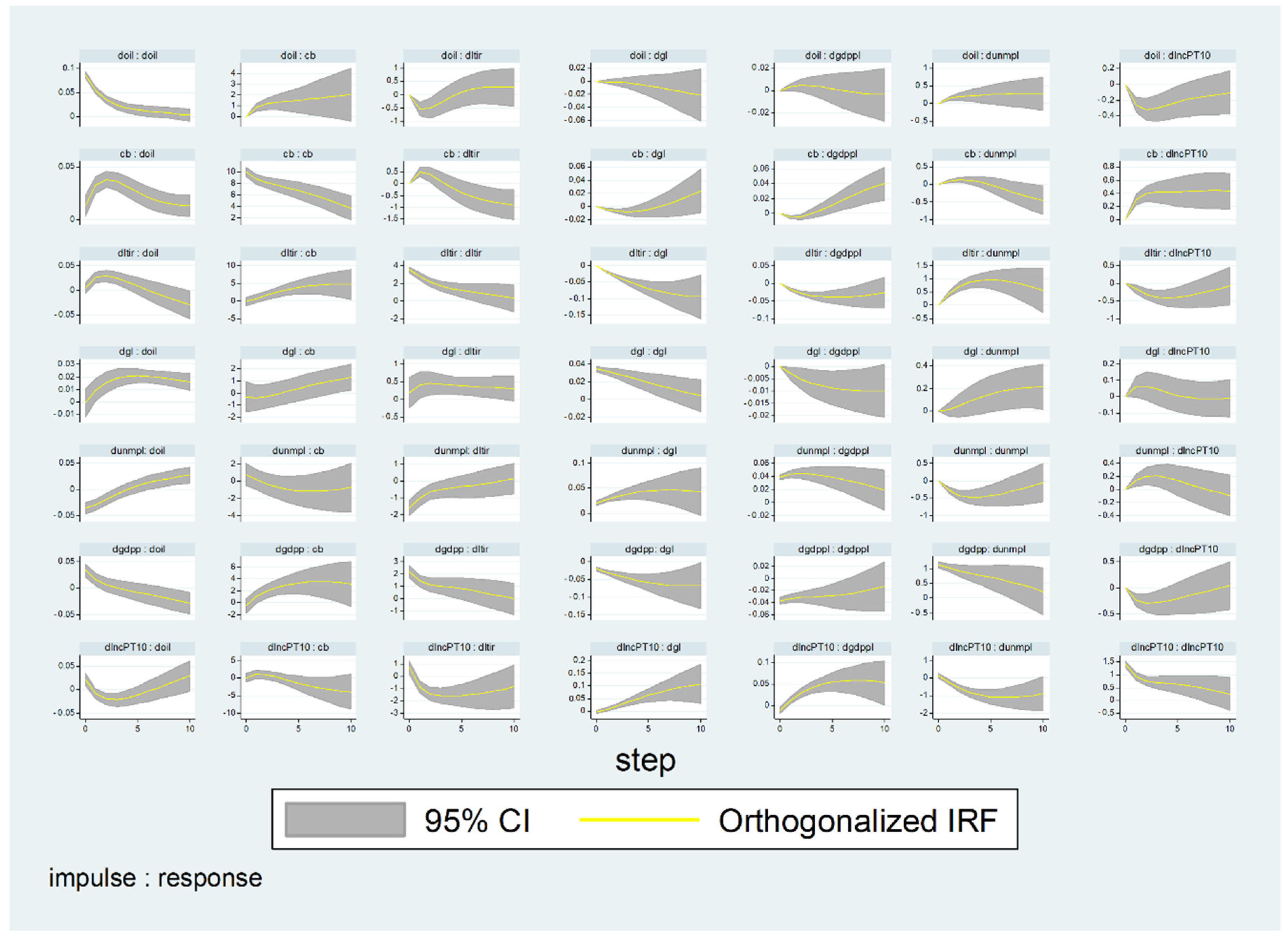
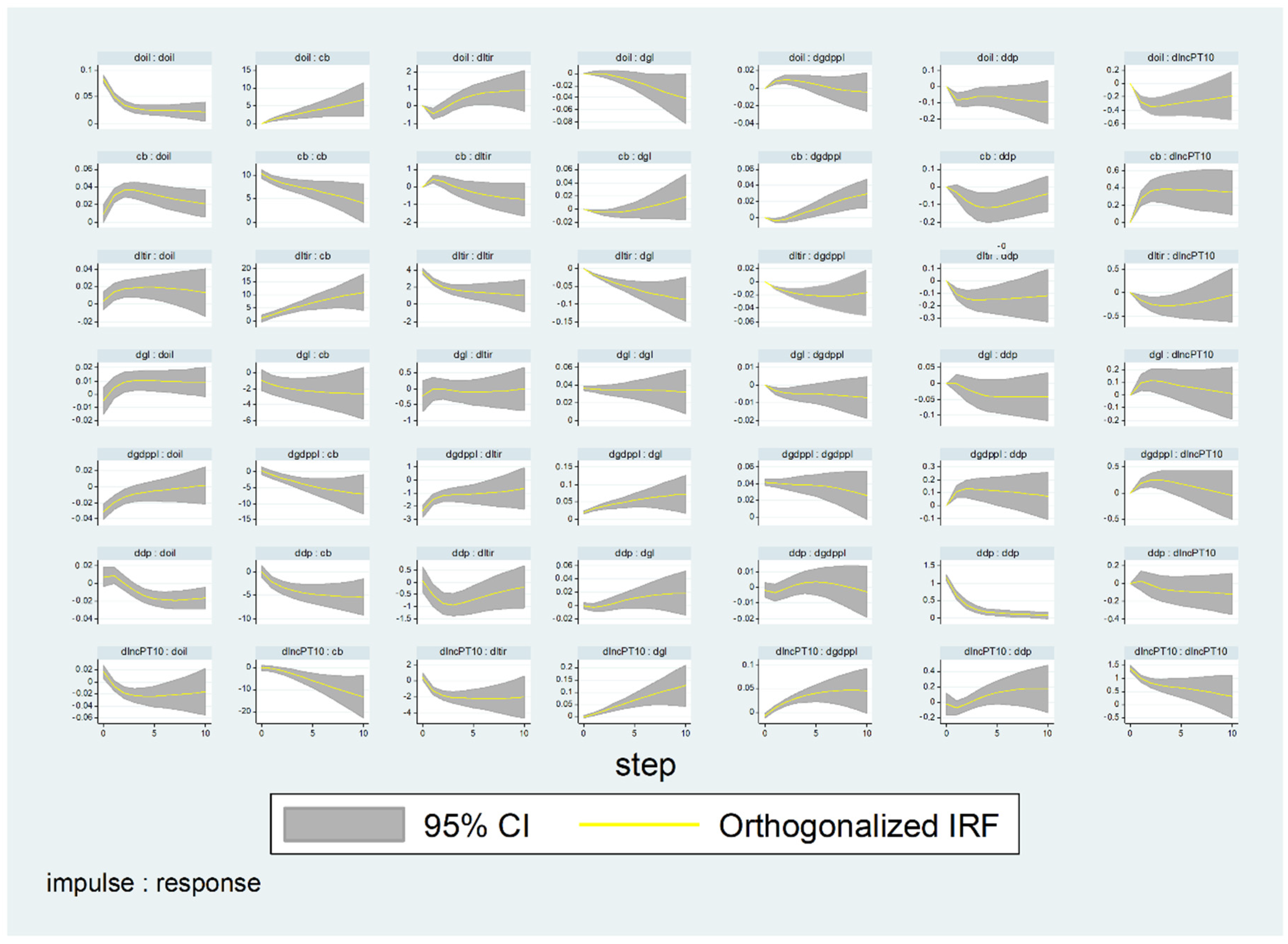
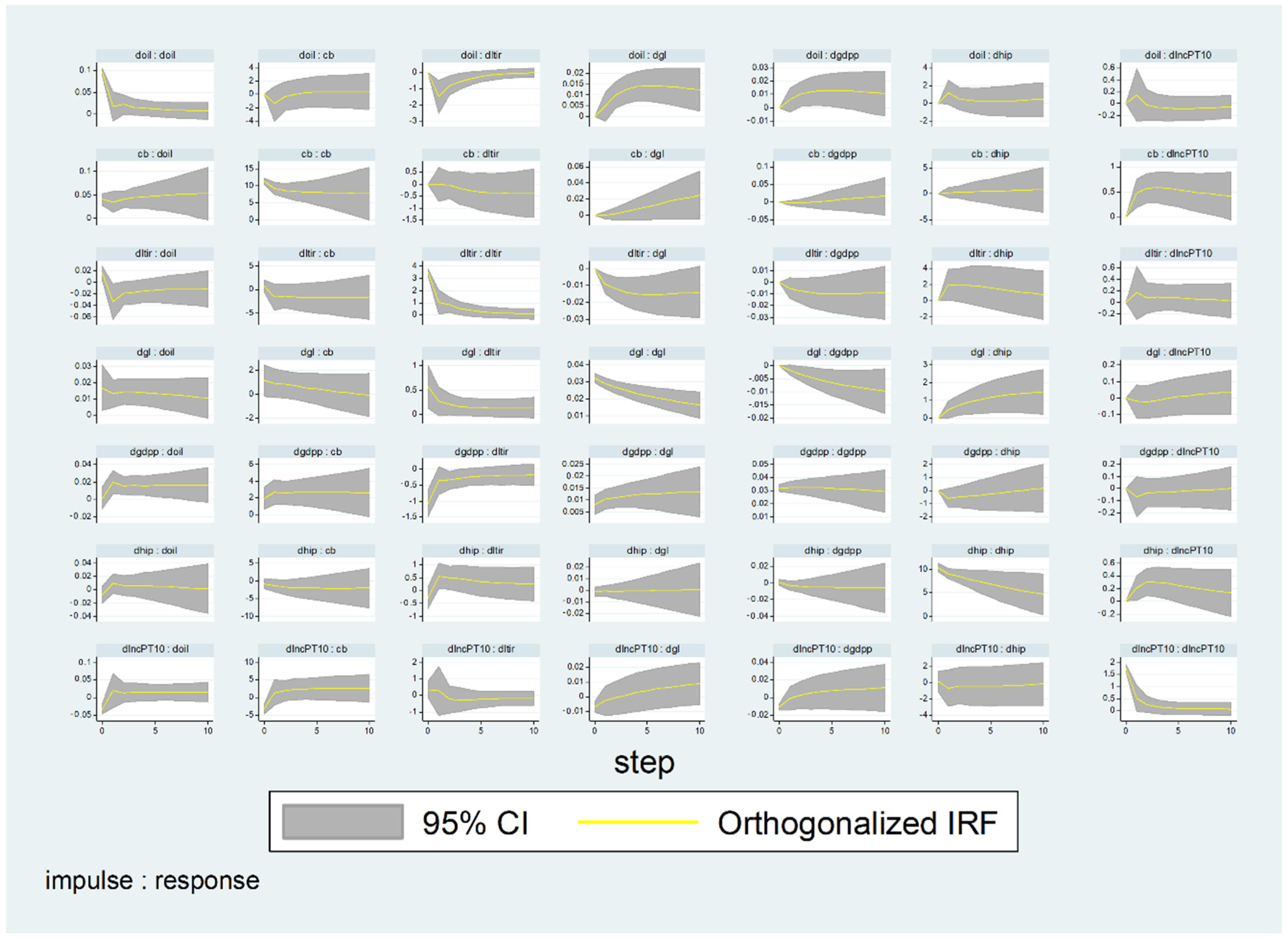
4.2. The Results of the PVAR and Interpretations

We constructed the IRFs using the PVAR as they are more valuable than VAR coefficients in analysing dynamic interactions between variables which are orthogonalized. IRFs can offer important information about the consequences of the shock in one variable while keeping other variables constant. As a result, our discussion for all the channels is mostly centered around the IRF plots shown in Figure 2, which further depicts the IRFs for each variable in relation to a one-standard deviation shock in the other variables, as our study investigates the dynamic impact of the UMP on income inequality in emerging economies through the earnings heterogeneity, income composition, and portfolio channels.

The interest of this study is in the last row of Figure 2. Firstly, looking at the dynamic impact of the UMP on income inequality (dgini) through the earnings heterogeneity channel (dunmpl) in the last row of Figure 2a, it shows that income inequality responds positively to an unexpected 1% shock on dunmpl. The UMP has an increasing impact on income inequality of about 0.5% from period zero to period seven through the earnings heterogeneity channel. This then converges to positive but above the steady-state region, after which it reverses back to negative. Based on the impulse response, results signify that the UMP has a long-run positive effect on income inequality through earnings heterogeneity channel. We documented similar results even when we adopted the pre-tax income held by the top 10% (PTI10%) collected from the World Inequality Database (see Appendix A in Figure A2). The possible logic behind the positive response on income inequality, could reflect the impact that MP Unemployment appears to be the most important cause of increasing earnings inequality during the whole period in which we used the Gini coefficient. The price effect also increases labor earnings inequality. Our empirical findings support what has been reported in the empirical literature, as the study by Coibion et al. (2017) for US countries, Furceri et al. (2018) for panel data from 32 advanced and emerging market countries and Hohberger et al. (2020) for Euro Area. These studies argue that a contractionary monetary policy of increases in official interest rates leads to an increase in unemployment which then pushes up income inequality (earnings heterogeneity channel).

On the other hand, we adopted a portfolio channel, captured by a house price index (dhip) to investigate the dynamic shock of the UMP on income inequality (dgini). Figure 2b in the last row shows that following a 1% standard deviation shock on dhip initially had a positive impact on income inequality of about 9% from period zero to period three. This then converged to a negative, but above the steady-state region, after which it reversed back to a steady-state region. The impulse response signifies that there is a short-run positive impact of an unexpected shock on the UMP (portfolio channel). When we adopted the pre-tax income held by the top 10% (PTI10%) collected from the World Inequality Database, the study documented similar results (see Appendix A in Figure A3). The possible reason for the positive impact of the UMP on income inequality through the portfolio composition channel is that this channel is related to the fact that a fall in interest rates impacts households’ asset holdings. Low-income households have more cash to satisfy their daily obligations than high-income households, which may save far more. In this situation, the UMP through the portfolio channel may raise inequality as financial assets rise. Furthermore, our findings support the findings reported by Saiki and Frost (2014) and Inui et al. (2017) for Japan, Domanski et al. (2016) for some countries in the Eurozone, Berisha et al. (2018) and Dolado et al. (2021) for the US.

Lastly, we adopted the equity index (dcba) as proxy for the income composition channel to investigate the dynamic shock of the UMP on income inequality. In the last row Figure 2c depicts the IRFs which we documented that, following a one percent standard deviation shock on dcba, initially had a positive impact on income inequality of about 10% from period zero to period four. This then converged to negative, but above the steady-state region, after which it reversed back to positive. The impulse response signifies that there is a long-run positive impact of an unexpected shock on unconventional monetary policy through the income composition on income inequality. The findings of the income composition channel are robust because we documented similar results even when we adopted the pre-tax income held by the top 10% (PTI10%) collected from the World Inequality Database to measure income inequality (see Appendix A in Figure A4).

Households obtain their incomes from different sources, each of which may respond differently to changes in monetary policy.

At the low end of the income distribution, households tend to rely more on transfer income (like unemployment benefits and food stamps), while households close to the median will rely on labor income and those in the upper part of the income distribution will rely relatively more on business and capital income. If a fall in interest rates stimulates economic activity, expansionary monetary policy may result in increased wages and decreased unemployment, thereby increasing inequality at the lower end of the distribution, as transfer income will vary little with economic activity. On the other hand, lower interest rates decrease interest income (mostly accruing to wealthier households), and inequality at the top of the distribution may decrease. In a nutshell, this demonstrates that the households with a higher proportion of interest income, which are normally the richest households, would benefit if an expansionary UMP shock increases assets and financial income more than wages. Similar findings were documented by Galbraith (1998), Coibion et al. (2012), Gornemann et al. (2012), Alves and Silva (2020) and Evgenidis and Fasianos (2021). The study by Gornemann et al. (2012) considers the importance of the earnings and income composition channels in the context of a model in which households differ in their employment status, earnings, and wealth. They find that the redistributive effects of monetary policy are such that contractionary monetary policy shocks increase inequality. The unemployed, in particular, are made worse off by monetary policy tightening, as a contractionary shock tends to prolong their unemployment spell, since firms reduce labor demand.

Our study further included the global variable in examining the dynamic impact of the UMP on income inequality for all channels. In our model, we controlled for an oil prices shock, in trying to trace how income inequality responds towards the oil price shock. We find that income inequality responds negatively to an unexpected 1% shock on a global variable (oil) and the response is significant in all channels. However, the oil price does not revert back to the steady state region. The possible clue might be the time horizon on our X-axis that is short. The argument for the negative impact is supported by the study documented by Sheng and Gupta (2021), where they disaggregate oil price shocks according to their origin into global economic ativity, oil supply, oil consumption demand, and oil inventory demand shocks, and test the dynamic response of income inequality to oil price structural shocks in United States. Their results indicate that supply shocks reduce income inequality in the medium and long term, but economic activity and oil inventory demand shocks mostly have a negative influence on income inequality over time.

For all channels we further control for real exchange rates (dtb), nominal interest rates (dstir), GDP per capita (dgdpp), and government expenditure (dg) as shown in Figure 2. In all channels we documented that, following a one percent standard deviation shock on dtb, they initially have a positive impact on income inequality and that the shock is positive only in the short run. Our results support the findings documented by Güzel and Arslan (2019) for Turkey, and by Jeanneney and Hua (2001) for China. A further positive response to income inequality was documented following a 1% standard deviation shock on the dstir of about 5%, 10%, and 4%, respectively, from period zero to period five, except for the income composition model where we found that the shock dies in period 10. Our finding supports the results of Berisha et al. (2018) for the US, and Diebold and Yilmaz (2012).

On the other hand, income inequality responds negatively following an unexpected 1% shock on dgdpp of about 10% in the earning heterogeneity model, 20% in the portfolio composition channel and 40% in the income composition channel. The impulse response signifies that there is a short-run negative impact of an unexpected shock on GDP per capita on income inequality. This finding supports the results documented by Wahiba and Weriemmi (2014), Lee et al. (2017), and Zungu et al. (2021) in the SADC region. In their study they documented that, below the threshold, per capita income decreases inequality. A further negative response on income inequality was documented following a 1% standard deviation shock on the dg of about 6% in the portfolio composition and 40% in the income composition model. The impulse response signifies a long-run negative impact of an unexpected shock of government expenditure on income inequality in income composition, while in the portfolio composition model it has a negative impact in the short run. This finding supports the results documented by Doumbia and Kinda (2019) for a panel of 83 countries, and Sánchez and Pérez-Corral (2018) for 28 member states of the European Union.

5. Conclusions

The existing empirical literature is marked by controversy surrounding the impact of unconventional monetary policy on income inequality in both advanced and emerging markets. The current paper seeks to fill the existing inconclusive in both theoretical and empirical ways by examining the current subject in emerging economics, focusing on the three unconventional monetary policy channels (heterogeneity, income composition, and portfolio composition channels), which we consider to be the most relevant monetary channels that may affect inequality dynamics differently; in a nutshell, by examining how the adopted unconventional monetary policies during the financial crisis triggered the nature of inequality in these countries. This is due to the rise in income and wealth inequality in the world in recent years, which has focused both politicians’ and policymakers’ concerns on the redistributive impacts of monetary policy. Moreover, it has been noted in the literature that most of the studies on this subject matter focus on the advanced market.

For this purpose, in this study, we utilized the PVAR model because of its advantages. One of the advantages is that it addresses the dynamics of numerous entities considered in parallel, which is significant for this type of study. These models are often deeper than standard VAR models since they not only examine the interaction between variables naively, as a conventional VAR model would, but they also add a cross-subsectional structure to the model. This allows us to differentiate common components from particular components, whether in terms of countries, variables, or time periods, etc., and then to utilize this structural knowledge to improve the accuracy of the estimation. It becomes much more resilient when dealing with data of uncertain quality and often short duration.

The estimation results provide sufficient evidence of a significant positive relationship between unconventional monetary policies and income inequality in emerging economies. We find that income inequality responds positively to an unexpected 1% shock in unconventional monetary policy through three channels: earnings heterogeneity channel, income composition channel, and portfolio composition channel. Then, for robustness purposes, we adopted two measures of income inequality, and these measures of income inequality responded positively to shocks on the UMP via the channels we used. The findings of the study show that income inequality responds positively to an unexpected shock on UMPs and its impact is significant and long-lasting. As a result, rising inequality may be explained by earning heterogeneity, income composition, and the portfolio channel. The results are theoretically plausible and consistent with the existing literature, such as Israel and Latsos (2019) for Japan, Albert et al. (2019) for the Eurozone and United States, Alves and Silva (2020) for the Euro Area, and Evgenidis and Fasianos (2021) for Great Britain.

We then added other macroeconomics variables to our model. Real GDP per capita, which was adopted to measure the standard of leaving or economic development. We find that income inequality responds negatively to an unexpected 1% shock in per capita income, which further validates the importance of improvement in the standard of living in these countries, as it was found to reduce income inequality in all channels. The results are theoretically plausible and consistent with the existing literature, such as by Güzel and Arslan (2019) for Turkey, and by Jeanneney and Hua (2001) for China. This shows that per capita income is an important factor in reducing income inequality in these countries, since there is a negative response to an unexpected shock to per capita income. Study further extend argument in this subject matter by controlling for fiscal policy instance through government expenditure. Income inequality responds negatively to an unexpected 1% shock in government expenditure during the period of portfolio channel and income-composition channel, while it is found to respond positively in the period of heterogeneity channel. We found that income inequality responds negatively to an unexpected 1% shock in per capita income, which validates that interest rates result in increased wages and decreased unemployment, thereby increasing inequality at the lower end of the distribution, as transfer income will vary little with economic activity. On the other hand, lower interest rates were found to decrease interest income (mostly accruing to wealthier households), and inequality at the top of the distribution may decrease. This demonstrates that the households with a higher proportion of interest income, which are normally the richest households, would benefit if an expansionary UMP shock increased assets and financial income more than wages. Similar findings were documented by Galbraith (1998), Coibion et al. (2012), Gornemann et al. (2012), Alves and Silva (2020), and Evgenidis and Fasianos (2021). We further incorporate the global variable in examining the dynamic impact of the UMP on income inequality for all channels. The global variables were controlled using oil prices. It was found that income inequality responds negatively to an unexpected 1% shock on a global variable and the response is significant in all channels.

It is evident that the central bank’s objective is and should be to fulfil its mandate of achieving maximum employment and price stability, thus bringing wide economic benefits. Furthermore, some forms of policies are more appropriate for addressing concerns about inequality (income policy or fiscal policy). However, the current study rings a bell for the central bank that monetary policies can have a wounding impact on income inequality. Therefore, the impact of monetary policies on income inequality should be considered when drafting or implementing these policies. We suggest that future research should try to find the possibility of the nonlinearity between unconventional and income inequality and further try to do a comparative study based on the region or level of development among countries.

References

1. Abrigo, Michael, and Inessa Love. 2016. Estimation of panel vector autoregression in Stata. The Stata Journal 16: 778–804. [Google Scholar] [CrossRef]
2. Acharya, Viral, Katharina Bergant, Matteo Crosignani, Tim Eisert, and Fergal McCann. 2017. The Anatomy of the Transmission of Macroprudential Policies: Evidence from Ireland. Presented at 16th International Conference on Credit Risk Evaluation, Interest Rates, Growth, and Regulation, Ireland, September; Available online: https://www.atlantafed.org/-/media/documents/news/conferences/2017/1102-financial-regulation-fit-for-the-future/acharya-bergant-crosignani-eisert-mccann.pdf (accessed on 24 February 2022).
3. Acharya, Viral, Katharina Bergant, Matteo Crosignani, Tim Eisert, and Fergal McCann. 2020. The Anatomy of the Transmission of Macroprudential Policies. IMF Working Papers. Washington, DC: IMF, vol. 2020, p. 58. [Google Scholar] [CrossRef]
4. Albert, Juan-Francisco, Nerea Gómez-Fernández, and Carlos Ochando. 2019. Effects of unconventional monetary policy on income and wealth distribution: Evidence from United States and Eurozone. Panoeconomicus 66: 535–58. [Google Scholar] [CrossRef]
5. Alvaredo, Facundo, Lucas Chancel, Thomas Piketty, Emmanuel Saez, and Gabriel Zucman. 2018. The elephant curve of global inequality and growth. AEA Papers and Proceedings 108: 103–8. [Google Scholar] [CrossRef]
6. Alves, José, and Tomás Silva. 2020. An Empirical Assessment of Monetary Policy Channels on Income and Wealth Disparities. REM Working Paper 0144-2020. Available online: https://rem.rc.iseg.ulisboa.pt/wps/pdf/REM_WP_0144_2020.pdf (accessed on 24 February 2022).
7. Amaral, Pedro. 2017. Monetary policy and inequality. In Economic Commentary. No. 1. Retrieved from Federal Reserve Bank of Cleveland Economic Commentary. Cleveland: Federal Reserve Bank of Cleveland. [Google Scholar]
8. Apanisile, Olumuyiwa Tolulope. 2021. Monetary policy shocks and income inequality in Nigeria: Do effects of anticipated and unanticipated shocks differ? African Journal of Economic Review 9: 1–18. [Google Scholar] [CrossRef]
9. Asteriou, Dimitris, and Stephen Hall. 2007. Applied Econometrics: A Modern Approach. New York: Palgrave Macmillan. [Google Scholar]
10. Atkinson, Tony. 2014. Public Economics in an Age of Austerity. New York: Routledge. [Google Scholar]
11. Batrancea, Larissa, Malar Mozhi Rathnaswamy, and Ioan Batrancea. 2021a. A panel data analysis of economic growth determinants in 34 African countries. Journal of Risk and Financial Management 14: 260. [Google Scholar] [CrossRef]
12. Batrancea, Larissa, Mircea Iosif Rus, Ema Speranta Masca, and Ioan Dan Morar. 2021b. Fiscal Pressure as a Trigger of Financial Performance for the Energy Industry: An Empirical Investigation across a 16-Year Period. Energies 14: 3769. [Google Scholar] [CrossRef]
13. Berisha, Edmond, John Meszaros, and Eric Olson. 2018. Income inequality, equities, household debt, and interest rates: Evidence from a century of data. Journal of International Money and Finance 80: 1–14. [Google Scholar] [CrossRef]
14. Bernanke, Ben. 2015. Monetary Policy and Inequality. Ben Bernanke’s Blog at Brookings. Washington, DC: White House. [Google Scholar]
15. Bhattacharya, Debapam. 2005. Asymptotic inference from multi-stage surveys. Journal of Econometrics 126: 145–71. [Google Scholar] [CrossRef]
16. Bivens, Josh. 2015. Gauging the Impact of the Fed on Inequality during the Great Recession”, Hutchins Center on fiscal & monetary Policy at Brooking’s. Working Paper 12. Available online: https://files.epi.org/2015/quantitative-easing-and-inequality-josh-bivens.pdf (accessed on 2 February 2022).
17. Bordo, Michael D., and Christopher M. Meissner. 2012. Does inequality lead to a financial crisis? Journal of International Money and Finance 31: 2147–61. [Google Scholar] [CrossRef]
18. Brunnermeier, Markus K., Thomas M. Eisenbach, and Yuliy Sannikov. 2012. Macroeconomics with Financial Frictions: A Survey. Available online: https://scholar.princeton.edu/sites/default/files/survey_macrofinance.pdf (accessed on 15 February 2022).
19. Bullard, James. 2014. Income Inequality and Monetary Policy: A Framework with Answers to Three Questions. Federal Reserve Bank of St. Louis. Available online: https://www.stlouisfed.org/-/media/project/frbstl/stlouisfed/Files/PDFs/Bullard/remarks/Bullard_CFR_26June2014_Final.pdf (accessed on 15 December 2021).
20. Carney, Mark. 2016. Speech by Mr Mark Carney, Governor of the Bank of England and Chairman of the Financial Stability Board, at the Bank of England. London. June 30. Available online: https://www.bis.org/review/r160704c.pdf (accessed on 15 December 2021).
21. Carpantier, Jean-Francois, Javier Olivera, and Philippe Van Kerm. 2018. Macroprudential policy and household wealth inequality. Journal of International Money and Finance 85: 262–77. [Google Scholar] [CrossRef]
22. Carpenter, Seth B., and William M. Rodgers III. 2004. The disparate labor market impacts of monetary policy. Journal of Policy Analysis and Management 23: 813–30. [Google Scholar] [CrossRef]
23. Casiraghi, Marco, Eugenio Gaiotti, Lisa Rodano, and Alessandro Secchi. 2018. A ‘reverse Robin Hood’? The distributional implications of non-standard monetary policy for Italian households. Journal of International Money and Finance 85: 215–35. [Google Scholar] [CrossRef]
24. Cerutti, Eugenio, Stijn Claessens, and Luc Laeven. 2017. The use and effectiveness of macroprudential policies: New evidence. Journal of Financial Stability 28: 203–24. [Google Scholar] [CrossRef]
25. Charemza, Wojaciech, and Derek Deadman. 1992. New Directions in Econometric Practice: General to Specific Modelling, Cointegration, and Vector Autoregression. Cheltenham: Edward Elgar Publishing, p. 370. [Google Scholar]
26. Coibion, Olivier, Yuriy Gorodnichenko, Lorenz Kueng, and John Silvia. 2012. Innocent Bystanders? Monetary Policy and Inequality in the U.S. NBER Working Paper, 18170. Available online: http://www.nber.org/papers/w18170 (accessed on 2 February 2022).
27. Coibion, Olivier, Yuriy Gorodnichenko, Lorenz Kueng, and John Silvia. 2017. Innocent Bystanders? Monetary Policy and Inequality. Journal of Monetary Economics 88: 70–89. [Google Scholar] [CrossRef]
28. Colciago, Andrea, Anna Samarina, and Jakob de Haan. 2019. Central bank policies and income and wealth inequality: A survey. Journal of Economic Surveys 33: 1199–231. [Google Scholar] [CrossRef]
29. Corak, Miles. 2013. Income Inequality, equality of opportunity, and intergenerational mobility. The Journal of Economic Perspectives 27: 79–102. [Google Scholar] [CrossRef]
30. Davtyan, Karen. 2016. Income Inequality and Monetary Policy: An Analysis of the Long Run Relation. Research Institute of Applied Economics Working Papers. vol. 4, pp. 1–37. Available online: https://www.ub.edu/irea/working_papers/2016/201604.pdf (accessed on 21 January 2022).
31. Diebold, Francis X., and Kamil Yilmaz. 2012. Better to give than to receive: Predictive directional measurement of volatility spillovers. International Journal of Forecasting 28: 57–66. [Google Scholar] [CrossRef]
32. Doepke, Matthias, and Martin Schneider. 2006. Inflation and the redistribution of nominal wealth. Journal of Political Economy 114: 1069–97. [Google Scholar] [CrossRef]
33. Dolado, Juan J., Gergő Motyovszki, and Evi Pappa. 2021. Monetary policy and inequality under labor market frictions and capital-skill complementarity. American Economic Journal: Macroeconomics 13: 292–332. [Google Scholar] [CrossRef]
34. Domanski, Dietrich, Michela Scatigna, and Anna Zabai. 2016. Wealth Inequality and Monetary Policy. BIS Quarterly Review. Available online: https://papers.ssrn.com/sol3/papers.cfm?abstract_id=2744862 (accessed on 10 June 2022).
35. Doumbia, Djeneba, and Tidiane Kinda. 2019. Reallocating Public Spending to Reduce Income Inequality: Can It Work? IMF Working Paper No. 19/188. Available online: https://ssrn.com/abstract=3471379 (accessed on 20 February 2022).
36. El Herradi, Mehdi, and Aurélien Leroy. 2019. Monetary Policy and the Top One Percent: Evidence from a Century of Modern Economic History. De Nederlandsche Bank Working Paper No. 632 (2019). Available online: https://ssrn.com/abstract=3379740 (accessed on 10 June 2022).
37. Erosa, Andrés, and Gustavo Ventura. 2002. On inflation as a regressive consumption tax. Journal of Monetary Economics 49: 761–95. [Google Scholar] [CrossRef]
38. Evgenidis, Anastasios, and Apostolos Fasianos. 2021. Unconventional Monetary Policy and Wealth Inequalities in Great Britain. Oxford Bulletin of Economics and Statistics 83: 115–75. [Google Scholar] [CrossRef]
39. Frees, Edward. 1995. Assessing cross-sectional correlation in panel data. Journal of Econometrics 69: 393–414. [Google Scholar] [CrossRef]
40. Friedman, Milton. 1937. The use of ranks to avoid the assumption of normality implicit in the analysis of variance. Journal of the American Statistical Association 32: 675–701. [Google Scholar] [CrossRef]
41. Frost, Jon, and René van Stralen. 2018. Macroprudential policy and income inequality. Journal of International Money and Finance 85: 278–90. [Google Scholar] [CrossRef]
42. Furceri, Davide, Prakash Loungani, and Aleksandra Zdzienicka. 2018. The effects of monetary policy shocks on inequality. Journal of International Money and Finance 85: 168–86. [Google Scholar] [CrossRef]
43. Galbraith, James. 1998. Created Unequal: The Crisis in American Pay. New York: Free Press. [Google Scholar]
44. Gambacorta, Leonardo, Boris Hofmann, and Gert Peersman. 2012. The Effectiveness of Unconventional Monetary Policy at the Zero Lower Bound: A Cross-Country Analysis. BIS Working Paper No. 384. Basel: Bank of International Settlements. [Google Scholar]
45. Gornemann, Nils, Keith Kuester, and Makoto Nakajima. 2012. Monetary Policy with Heterogeneous Agents. FRB of Philadelphia Working Paper No. 12-21. Available online: https://ssrn.com/abstract=2147841 (accessed on 10 June 2022).
46. Guerello, Chiara. 2018. Conventional and unconventional monetary policy vs. household’s income distribution: An empirical analysis for the Euro Area. Journal of International Money and Finance 85: 187–214. [Google Scholar] [CrossRef]
47. Güzel, Arif Eser, and Ünal Arslan. 2019. On the nexus between exchange rate and income distribution in Turkey: ARDL bound testing analysis. Economic Journal of Emerging Markets 11: 1–7. [Google Scholar] [CrossRef]
48. Harris, Richard D. F., and Elias Tzavalis. 1999. Inference for unit roots in dynamic panels where the time dimension is fixed. Journal of Econometrics 91: 201–26. [Google Scholar] [CrossRef]
49. Heathcote, Jonathan, Fabrizio Perri, and Giovanni L. Violante. 2010. Unequal we stand: An empirical analysis of economic inequality in the United States, 1967–2006. Review of Economic Dynamics 13: 15–51. [Google Scholar] [CrossRef]
50. Hohberger, Stefan, Romanos Priftis, and Lukas Vogel. 2020. The distributional effects of conventional monetary policy and quantitative easing: Evidence from an estimated DSGE model. Journal of Banking & Finance 113: 105483. [Google Scholar] [CrossRef]
51. Huber, Evelyne, and John D. Stephens. 2014. Income inequality and redistribution in post-industrial democracies: Demographic, economic and political determinants. Socio-Economic Review 12: 245–67. [Google Scholar] [CrossRef]
52. Im, Kyung So, M. Hashem Pesaran, and Yongcheol Shin. 2003. Testing for unit roots in heterogeneous panels. Journal of Econometrics 115: 53–74. [Google Scholar] [CrossRef]
53. Inui, Masayuki, Nao Sudou, and Tomoaki Yamada. 2017. Effects of Monetary Policy Shocks on Inequality in Japan. Bank of Japan Working Paper 17-e-3. Available online: https://ssrn.com/abstract=2982887 (accessed on 3 January 2022).
54. Israel, Karl-Friedrich, and Sophia Latsos. 2019. The Impact of (un)Conventional Expansionary Monetary Policy on Income Inequality—Lessons from Japan. Working Paper, No. 163. Leipzig: Universität Leipzig, Wirtschaftswissenschaftliche Fakultät. [Google Scholar]
55. Jeanneney, S. Guillaumont, and Ping Hua. 2001. How does real exchange rate influence income inequality between urban and rural areas in China? Journal of Development Economics 64: 529–45. [Google Scholar] [CrossRef]
56. Kimura, Takeshi, and Jouchi Nakajima. 2016. Identifying conventional and unconventional monetary policy shocks: A latent threshold approach. The B.E. Journal of Macroeconomics 16: 277–300. [Google Scholar] [CrossRef]
57. Konstantinou, Panagiotis, Anastasios Rizos, and Artemis Stratopoulou. 2022. Macroprudential policies and income inequality in former transition economies. Economic Change and Restructuring 55: 1005–62. [Google Scholar] [CrossRef]
58. Kumhof, Michael, Romain Rancière, and Pablo Winant. 2015. Inequality, leverage and crises. American Economic Review 105: 1217–45. [Google Scholar] [CrossRef]
59. Lee, Yoke Yee, Hui Xin Lim, Sock Hun Lim, and Yie Tien Quek. 2017. Income Distribution and Economic Growth: A Panel Data Analysis. Unpublished Bachelor’s thesis, University Tunku Rahman, Pulau Pinang, Malaysia. [Google Scholar]
60. Lenza, Michele, and Jiri Slacalek. 2019. How Does Monetary Policy Affect Income and Wealth Inequality? Evidence from Quantitative Easing in the Euro Area. ECB Working Paper Series No 2190/October 201. Luxembourg: EU Publications. [Google Scholar] [CrossRef]
61. Mumtaz, Haroon, and Angeliki Theophilopoulou. 2017. The impact of monetary policy on inequality in the UK. An empirical analysis. European Economic Review 98: 410–23. [Google Scholar] [CrossRef]
62. Nakajima, Makoto. 2015. Business Cycles in the Equilibrium Model of Labor Market Search and Self-insurance. International Economic Review 53: 399–432. [Google Scholar] [CrossRef]
63. OECD (Organization for Economic Cooperation and Development—OECD). 2014. Society at a Glance 2014: OECD Social Indicators. Paris: OECD Publishing, pp. 1–143. [Google Scholar]
64. Pesaran, Hashen. 2004. General Diagnostic Tests for Cross-Sectional Dependence in Panels. Cambridge Working Papers in Economics No. 0435. Cambridge: Faculty of Economics, The University of Cambridge. [Google Scholar] [CrossRef]
65. Piketty, Thomas. 2014. “Capital in the 21st Century”. Cambridge: Harvard University Press. [Google Scholar]
66. Rajan, Raghuram. 2010. “Fault Lines: How Hidden Fractures Still Threaten the World Economy”. Princeton: Princeton University Press. [Google Scholar]
67. Romer, Christina D., and David H. Romer. 1999. Monetary policy and the well-being of the poor. Economic Review 84: 21–49. [Google Scholar]
68. Rupprecht, Manuel. 2020. Income and wealth of euro area households in times of ultra-loose monetary policy: Stylised facts from new national and financial accounts data. Austrian Institute for Economic Research 47: 281–302. [Google Scholar] [CrossRef]
69. Saiki, Ayako, and Jon Frost. 2014. Does unconventional monetary policy affect inequality? Evidence from Japan. Applied Economics 46: 4445–54. [Google Scholar] [CrossRef]
70. Sánchez, Angeles, and Antonio L. Pérez-Corral. 2018. Government social expenditure and income inequalities in the European Union. Review of Public Economics 227: 133–56. Available online: https://ideas.repec.org/a/hpe/journl/y2018v227i4p133-156.html (accessed on 28 April 2022).
71. Sarfati, Hedva. 2016. OECD. In it together: Why less inequality benefits all. Paris, 2015. p. 332 ISBN 978–264-23266-2. International Social Security Review 68: 115–17. [Google Scholar] [CrossRef]
72. Sheng, Xin, and Rangan Gupta. 2021. The Impact of Oil Price Shocks on Income Inequality: Evidence from State-Level Data of the United States. Working Papers 202128. Department of Economics, University of Pretoria. Available online: https://www.up.ac.za/media/shared/61/WP/wp_2022_17.zp217507.pdf (accessed on 3 April 2022).
73. Solt, Frederick. 2020. The standardized world Income-inequality database. Social Science Quarterly 90: 231–42. [Google Scholar] [CrossRef]
74. Taghizadeh-Hesary, Farhad, Naoyuki Yoshino, and Sayoko Shimizu. 2018. The Impact of Monetary and Tax Policy on Income Inequality in Japan. ADBI Working Paper 837. Tokyo: Asian Development Bank Institute. Available online: https://www.researchgate.net/publication/325967488_The_Impact_of_Monetary_and_Tax_Policy_on_Income_Inequality_in_Japan (accessed on 23 April 2022).
75. Tzur-Ilan, Nitzan. 2016. The effect of credit constraints on housing choices: The case of LTV limits. Presented at Bank of Israel Research Department Conference, Jerusalem, Israel, December; Available online: https://www.boi.org.il/he/newsandpublications/pressreleases/documents/%D7%A0%D7%99%D7%A6%D7%9F%20%D7%A6%D7%95%D7%A8%20%D7%90%D7%99%D7%9C%D7%9F.pdf (accessed on 10 June 2022).
76. Wahiba, Nasfi Fkili, and Malek El Weriemmi. 2014. The relationship between Economic growth and income inequality. International Journal of Economics and Financial Issues 4: 135–43. [Google Scholar]
77. Wilkinson, Richard, and Kate Pickett. 2009. The Spirit Level: Why More Equal Societies Almost Always a Bette. Edited by S. Tuters. London: Allen Lane. [Google Scholar]
78. Williamson, Stephen. 2009. Monetary policy and distribution. Journal of Monetary Economics 55: 1038–53. [Google Scholar] [CrossRef]
79. World Development Indicators. 2022. World Bank. Washington, DC. Available online: http://data.worldbank.org/data-catalog/world-development-indicators (accessed on 3 January 2022).
80. Yellen, Chair Janet. 2014. Monetary Policy and Financial Stability; Michel Camdessus Central Banking Lecture. Washington, DC: International Monetary Fund. Available online: https://www.federalreserve.gov/newsevents/speech/yellen20140702a.htm (accessed on 20 January 2022).
81. Zinman, Janath. 2010. Restricting consumer credit access: Household survey evidence on effects around the Oregon rate cap. Journal of Banking and Finance 34: 546–56. [Google Scholar] [CrossRef]
82. Zungu, Lindokuhle Talent, and Lorraine Greyling. 2022. Investigating the asymmetric effect of income inequality on financial fragility in South Africa and selected emerging markets: A Bayesian approach with hierarchical priors. Asian Journal of Economics and Banking. forthcoming. [Google Scholar]
83. Zungu, Lindokuhle Talent, Lorraine Greyling, and Nkanyiso Mbatha. 2021. Economic growth and income inequality: A non-linear econometrics analysis of the SADC region, 1995–2015. African Journal of Economic and Management Studies 12: 285–301. [Google Scholar] [CrossRef]
Figure 1. Eigenvalue stability condition. Note: All the eigenvalues lie inside the unit circle. PVAR satisfies stability condition. Source: Author’s illustration based on SWIID (Solt 2020; World Development Indicators 2022).
Socsci 11 00369 g001
Figure 2. (a) Response of inequality on unconventional monetary policy (heterogeneity channel). (b) Response of inequality on unconventional monetary policy (portfolio channel). (c) Response of inequality on unconventional monetary policy (Income-composition) channel. Note: The shaded areas refer to the 95% confidence band. Moreover, the IRFs present two periods, which are a short run from zero to four years and a long run from five to 10 years. Therefore, the orthogonalised IRF is interpreted as aligned with the short-run and long-run periods, as defined. Source: Author’s illustration based on SWIID (Solt 2020; World Development Indicators 2022).
Socsci 11 00369 g002aSocsci 11 00369 g002b