1. Introduction
Long-span bridge structures can be affected by various environmental factors during their long-term operations, among which the temperature effect is particularly significant [
1,
2,
3]. In recent years, numerous studies on bridge temperature effects have been carried out [
4,
5,
6,
7], mostly considering uniform temperature fields. Some scholars [
8,
9] have studied the influence of boundary factors such as solar radiation on the bridge temperature field. Some scholars [
10,
11,
12,
13] studied the time-varying temperature distribution of bridges and established a temperature gradient distribution model. There have also been numerous scholars [
14,
15,
16,
17,
18,
19,
20] who have studied the long-term measured cross-section temperatures of a large number of bridges with different cross-section forms, observed transverse temperature gradients and proposed two-dimensional temperature field calculation models.
It is worth noting that the above studies are based on the assumption that the temperature is uniformly distributed along the longitudinal span direction of the bridge. However, in actual engineering, the temperature field of large-scale structures, such as long-span bridges, is usually non-uniform. It has been shown that the stresses and deformations caused by non-uniform temperature distribution can be comparable to those caused by static and live loads, which may also cause cracks and excessive deformations [
21,
22,
23,
24,
25].
Actually, the existing standards [
26,
27,
28,
29,
30] have neglected the influence of the longitudinal non-uniform temperature distribution on bridges, assuming that the temperature field can be represented by one-point measuring data, i.e., a uniform distribution field. Although this assumption simplifies the analysis of bridges affected by temperature in the two-dimensional plane, it may overestimate the temperature effects at some spanwise locations and underestimate them at others. Moreover, the nonlinear effects caused by temperature effects are neglected by the uniform-distribution assumption [
31,
32]. Therefore, the temperature effects cannot be accurately evaluated when adopting the above assumption. Additionally, the inability to accurately assess the temperature effects of large-span bridges may bring uncertainty to the bridge during the design, construction and operation stages, thus affecting the structural safety of the bridge [
33,
34].
Therefore, the longitudinal temperature distribution is important for the accurate analysis of bridge temperature effects. Several studies have started to pay attention to this topic. Abid et al. [
35] investigated the temperature distribution of bridge segmental models under the influence of solar radiation and air temperature variations through numerical simulations. Based on the health monitoring data of the Aizhai Bridge, Hu et al. [
36] found that there were temperature differences at different measuring points along the longitudinal direction of the bridge span. Gu et al. [
37] proposed a vertical and lateral temperature gradient model for different longitudinal positions along the bridge span. Liu et al. [
38] studied the non-uniform longitudinal distribution temperature of concrete-filled steel tubular bridges due to the change in component inclination. Although the above studies considered the variability of temperature distribution, it is limited to a single or several measuring points, and the conclusions may not be well applied to actual bridges. In this context, the longitudinal temperature distribution on the whole bridge and its statistical characteristics was insufficient. Moreover, the role of the non-uniform longitudinal distributions of temperature was not analyzed in depth.
Therefore, this work studies the longitudinal temperature distribution of steel box girders based on the field-measured temperature data. The main objective was to provide a more accurate description of the longitudinal temperature field of long-span bridges.
The paper is organized as follows. In
Section 2, the bridge and its health monitoring system are introduced. In
Section 3, the probability density characteristic analysis is carried out by selecting typical measuring points in the longitudinal direction of the bridge, and the probability density curves are fitted; next, the temperature of all measurement points is statistically analyzed, and longitudinal distribution curves are fitted; A correlation analysis was then performed, highlighting variability in the longitudinal direction. Finally, the frequency domain features were analyzed, and the space-time contour maps were given to study the mechanisms and processes of the non-uniform distribution of temperature.
2. Description of the Bridge and Its Monitoring System
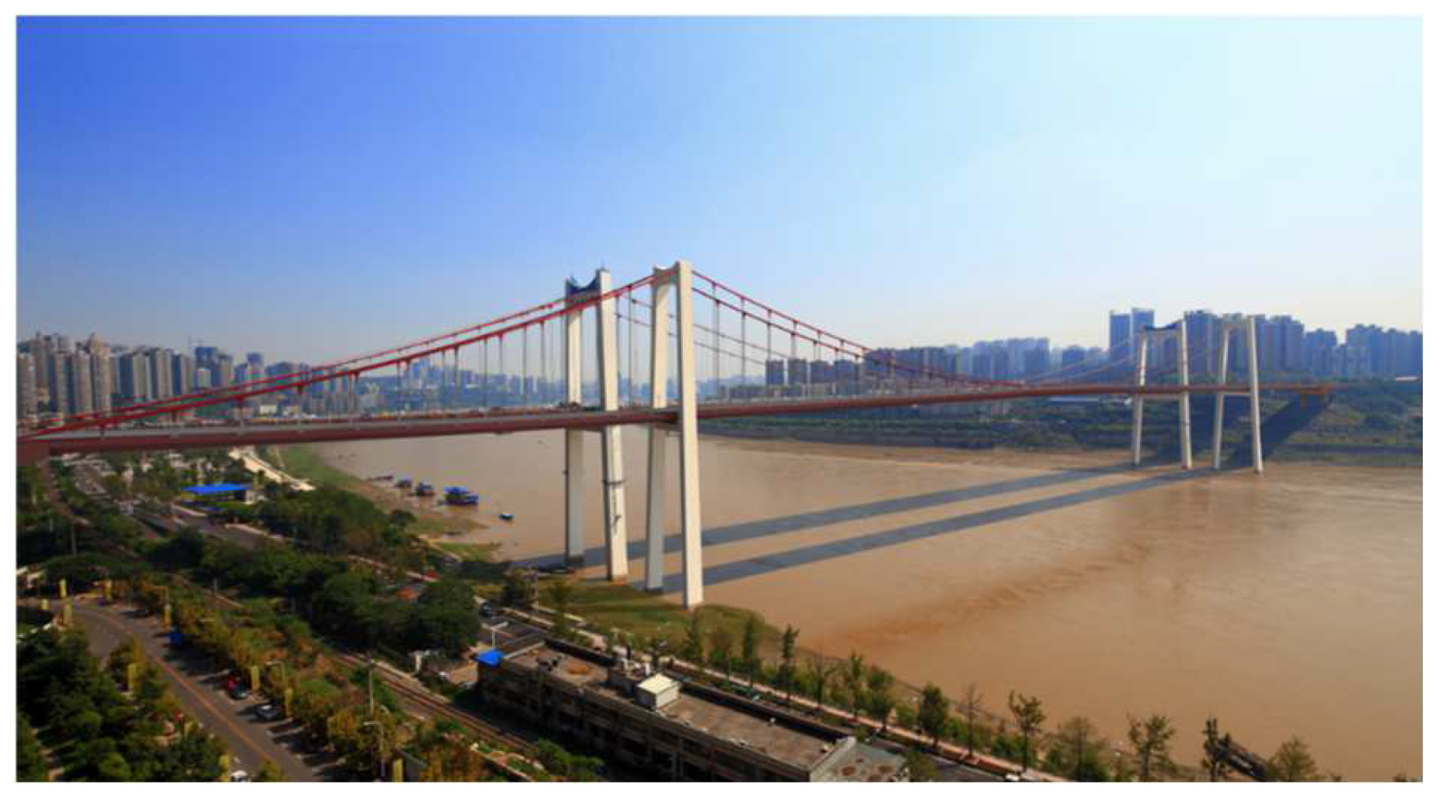
The Egongyan rail bridge is a long-span suspension bridge located in southwestern China and across the Yangtze River.
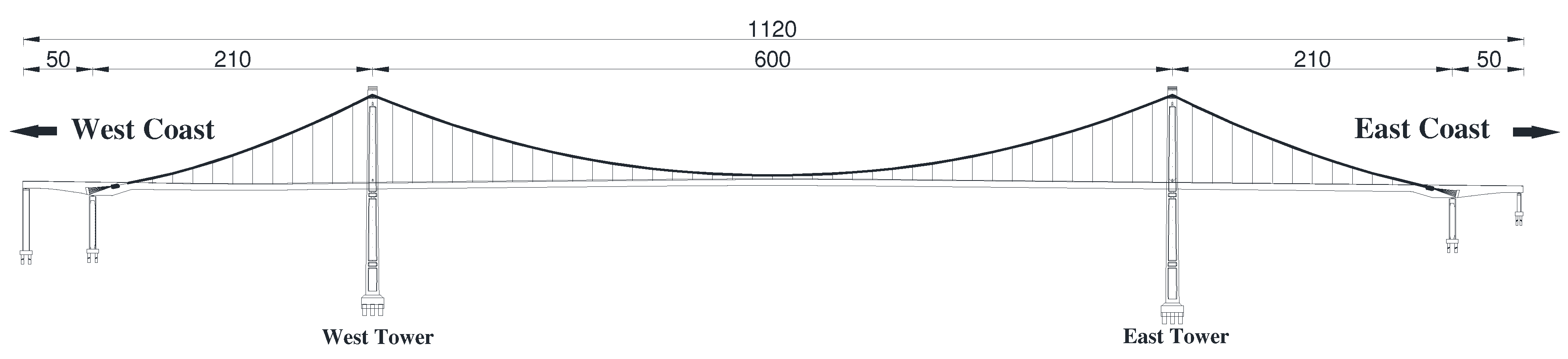
Figure 1 is a picture of this bridge, and
Figure 2 shows its elevated view. It is a five-span self-anchored suspension bridge with double towers and double plane cables. The middle three spans are the main bridge, and the extended span with a span of 50 m is the approach bridge. The overall length of the bridge is 1650.5 m, and the main span is 600 m. In addition, the main girder is a closed single-box five-chamber steel box girder structure [
39,
40,
41].
To monitor the operation status, a structural health monitoring system (SHMS) was installed on the Egongyan rail bridge [
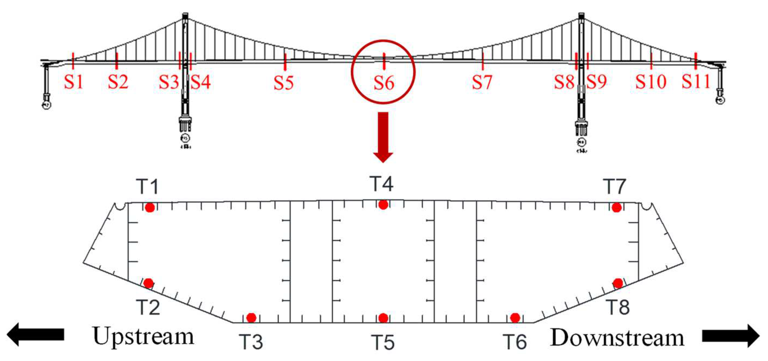
42] and has been in operation since 2020. A total of 267 sensors were installed at different parts of the bridge to collect various types of structural and environmental information. Among them, the temperature measuring points on the steel box girder of the main bridge were arranged symmetrically about the mid-span, as shown in
Figure 3. A total of 88 temperature sensors were installed at 11 sections (S1–S11) along the main bridge, and there were also eight measuring points (T1~T8) inside the surface of each section. Taking the mid-span section (S6); for instance, a plan view of the measuring point at each section is shown in
Figure 3.
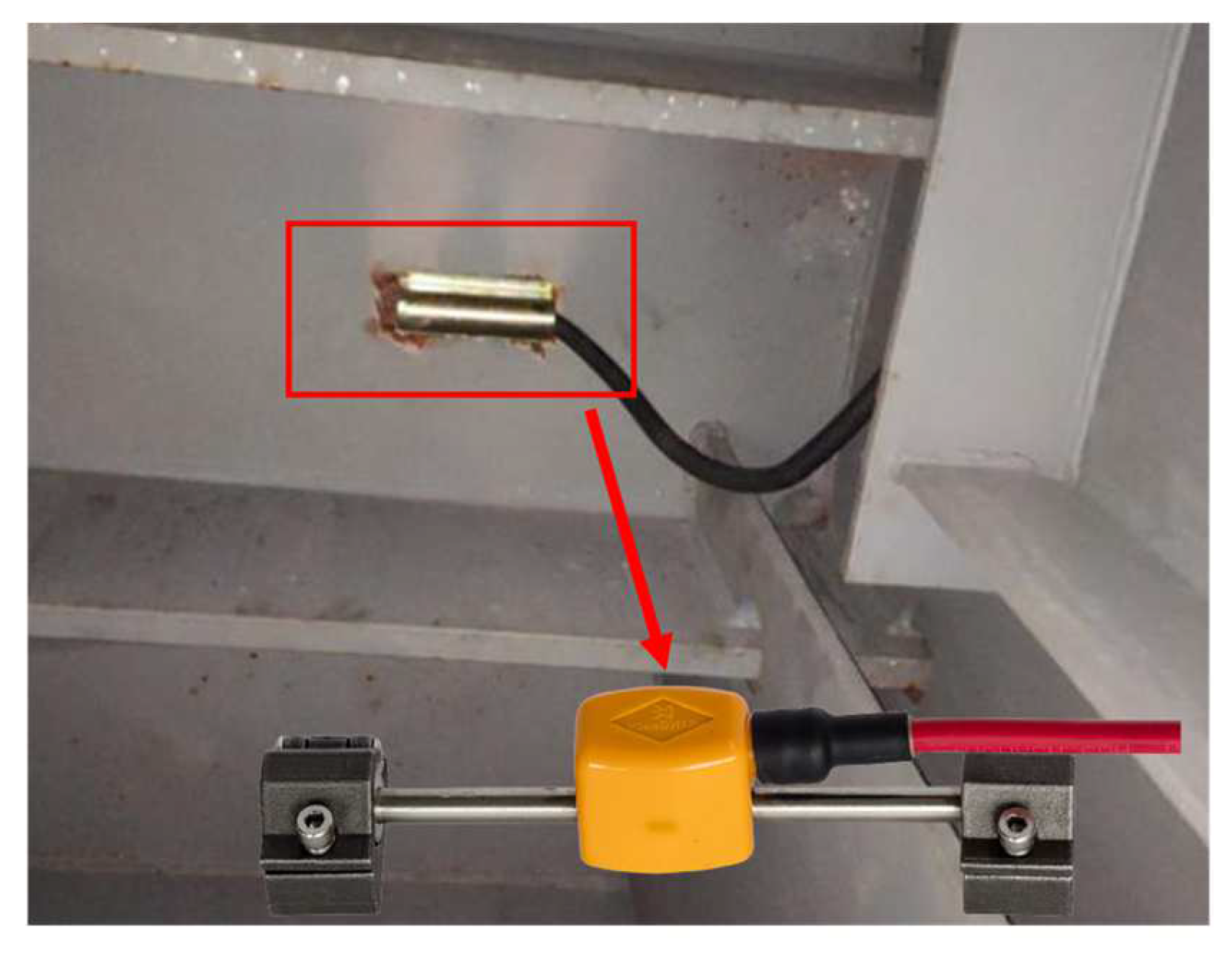
The surface temperature of the box girder was monitored using a JMZX-212HAT surface intelligent digital tandem strain gauge with built-in temperature sensors as the testing instrument [
43], as shown in
Figure 4. The main technical parameters of the sensor were as follows: Operating ambient temperature: −40 °C~+80 °C; Temperature measurement range: −20 °C~+80 °C; Temperature resolution: 0.1 °C; Temperature measurement accuracy: ±0.5 °C.
3. Probability Density Characteristics of Temperature
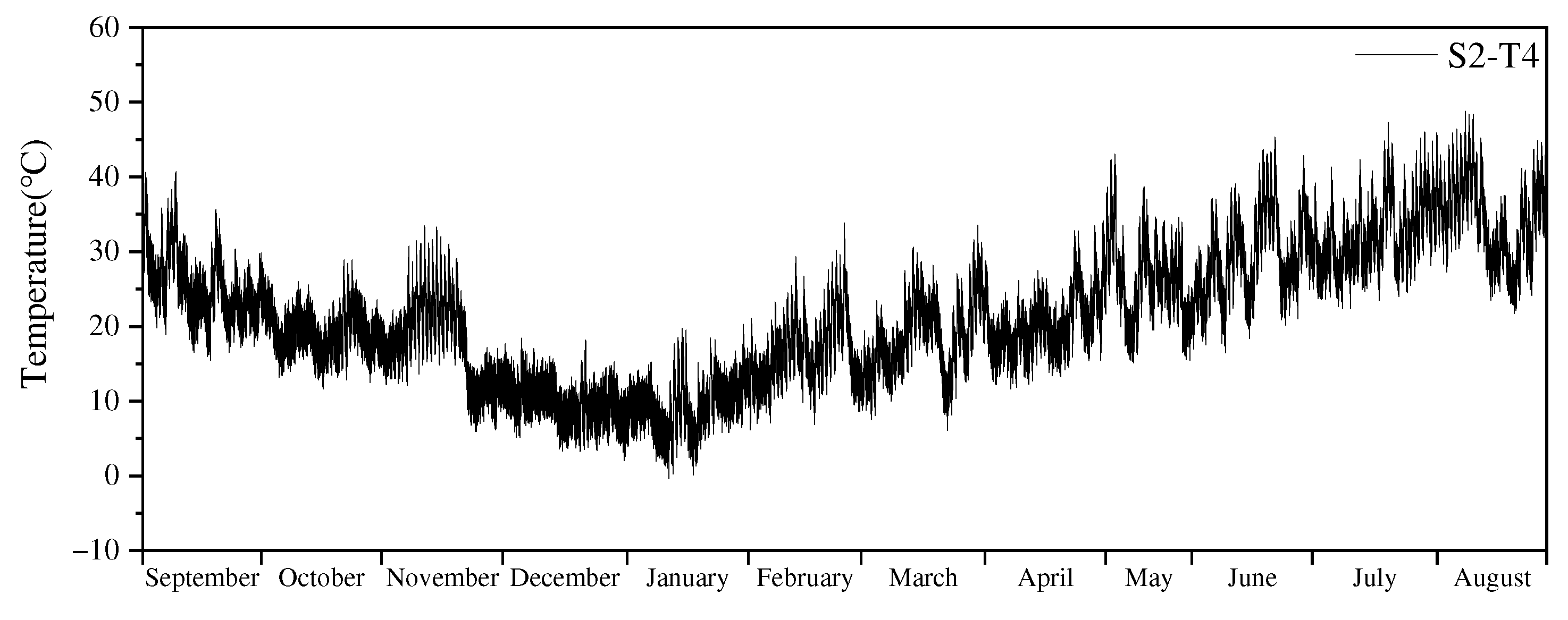
To display the annual variations in the girder surface temperature, the measuring point T4 at different longitudinal positions S2, S6 and S10 was chosen, for instance.
Figure 5 shows the monitoring data from 1 September 2020 to 31 August 2021. It can be observed that the annual temperature changes all appeared to have obvious periodic patterns, and this could be approximately described by sinusoidal functions, with lower temperatures from December to February and higher temperatures from June to August. In addition to the low-frequency periods, the temperature data also contained high-frequency fluctuations. High-frequency fluctuations may be due to the effect of daily temperature changes. In addition, it was found that the overall temperature value of S6 and its variance amplitude were significantly larger than those of S2 and S10, and the difference was more obvious in summer. This was a preliminary indication of the non-uniformity of the temperature distribution along the longitudinal direction of the bridge, which is discussed later.
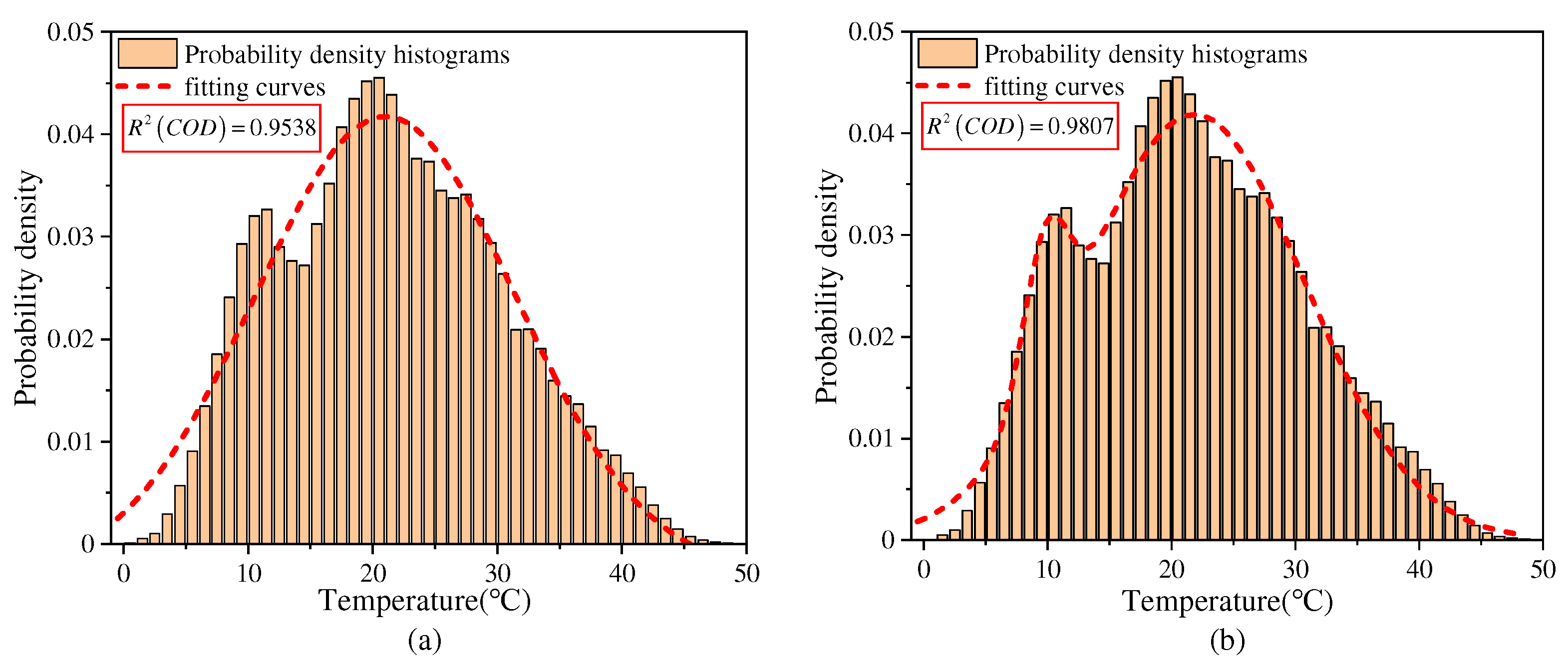
In previous studies, the Gaussian distribution model [
44,
45,
46] has been commonly used for fitting the probability density function (PDF) of the temperature. However, it is obvious in
Figure 6a that the PDF cannot be properly fitted by the Gaussian distribution model due to bimodal characteristics. By comparing the fitting results of several models, the weighted superposition of two normal distributions was selected for fitting the current data, with its mathematical expression as follows:
where
denotes the surface temperature of the steel box girder,
denotes the probability density model of
,
denotes the normal distribution function with the mean value
and the standard deviation
,
is the weight of the two normal distribution functions with
.
The goodness-of-fit for the different models is shown in
Figure 6. The
(coefficient of determination, COD) of the superposition of two normal distribution models was significantly higher than that of the Gaussian distribution model. Therefore, it was reasonable to choose the superposition of two normal distribution models to describe the probability distribution of temperature.
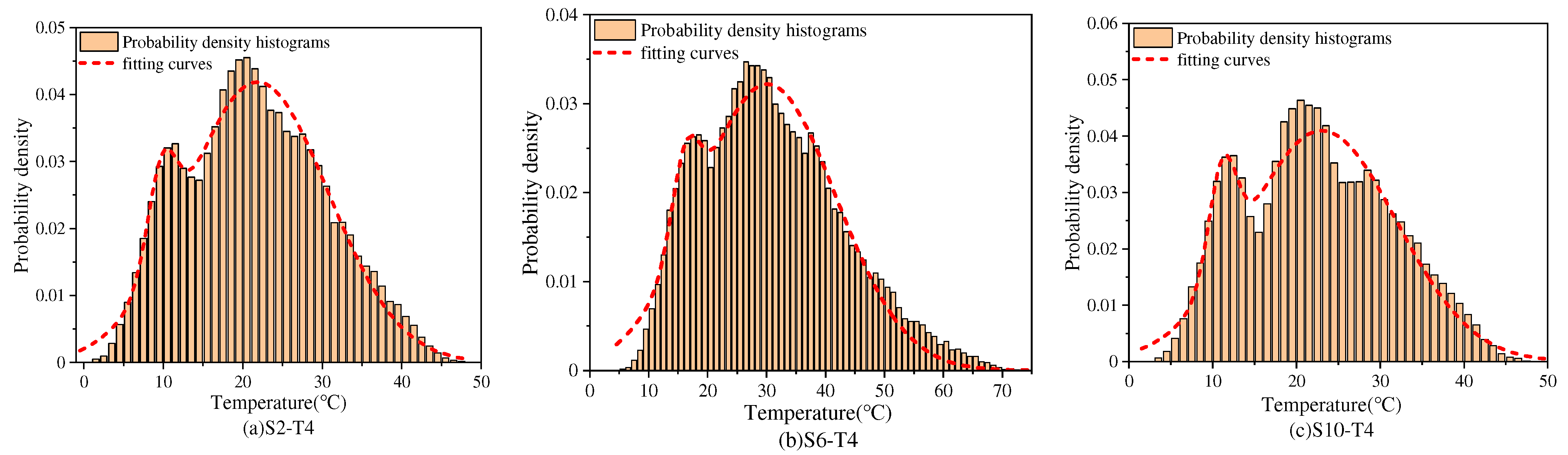
The probability density histograms of measuring points S2-T4, S6-T4 and S10-T4 and their fitted curves are shown in
Figure 7. It can be seen that the fitted curves were in good agreement with the measured ones. Meanwhile, the fitting results all passed the K-S test with a significance level
, indicating that the fitting curves could accurately describe the probability density characteristics of the surface temperature of the steel box girder. The results show that the probability density curves of each measuring point have bimodal characteristics. This was due to the bridge being located in the subtropical humid monsoon climate zone and its experience of a transition period between seasons. The temperatures at the two peaks represent the temperature during the spring-summer and summer-fall transitions and during the fall-winter and winter-spring transitions, respectively.
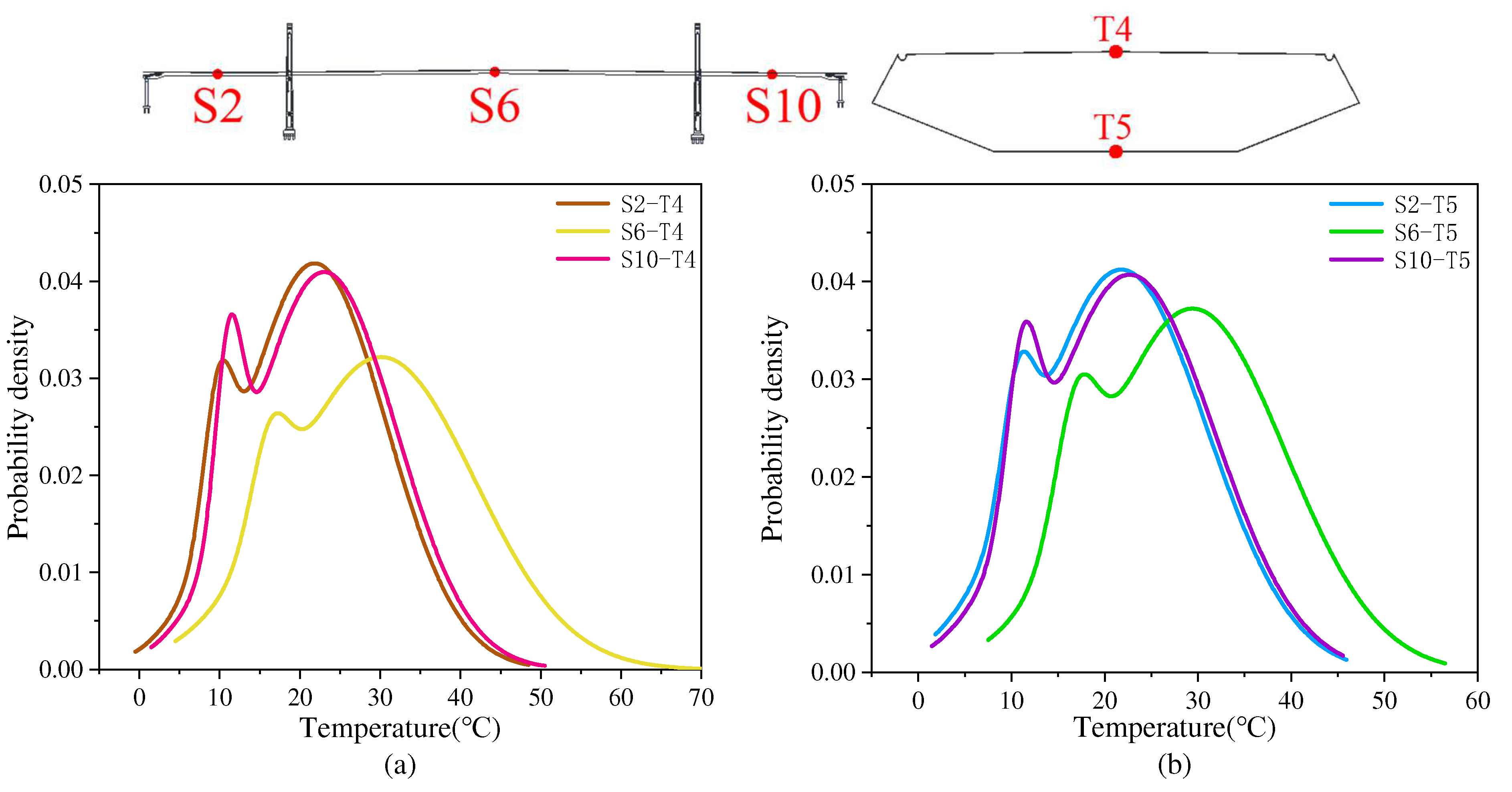
To investigate the difference in temperature distribution along the longitudinal direction of the bridge, the probability densities of T4 and T5 (on the top and bottom plates, respectively) and at different longitudinal sections S2, S6 and S10 were fitted based on the abovementioned model. The estimated floating parameters are shown in
Table 1, and the corresponding PDFs are given in
Figure 8.
From
Table 1 and
Figure 8, it can be seen that there was a significant difference between the PDFs of the mid-span and side-span for both the top and the bottom plates. Concerning the two peaks in the PDFs, the measuring point S6-T4 was mainly concentrated around 30 °C and 16 °C, while S10-T4 was mainly concentrated around 23 °C and 11 °C, indicating that there was a significant difference in the temperature distribution along the longitudinal direction of the bridge, and the temperature in the mid-span was significantly higher than that in the side span. Moreover, PDFs were not the same for the side-span measuring points, which were symmetrical along the bridge centerline, indicating a non-uniform longitudinal temperature distribution in the steel box girder. This phenomenon shows that the assumption of uniform temperature used in previous studies and specifications [
14,
20,
30] is not reasonable.
4. Statistical Analyses of Temperature Distribution along the Bridge
4.1. Temperature Longitudinal Distributions
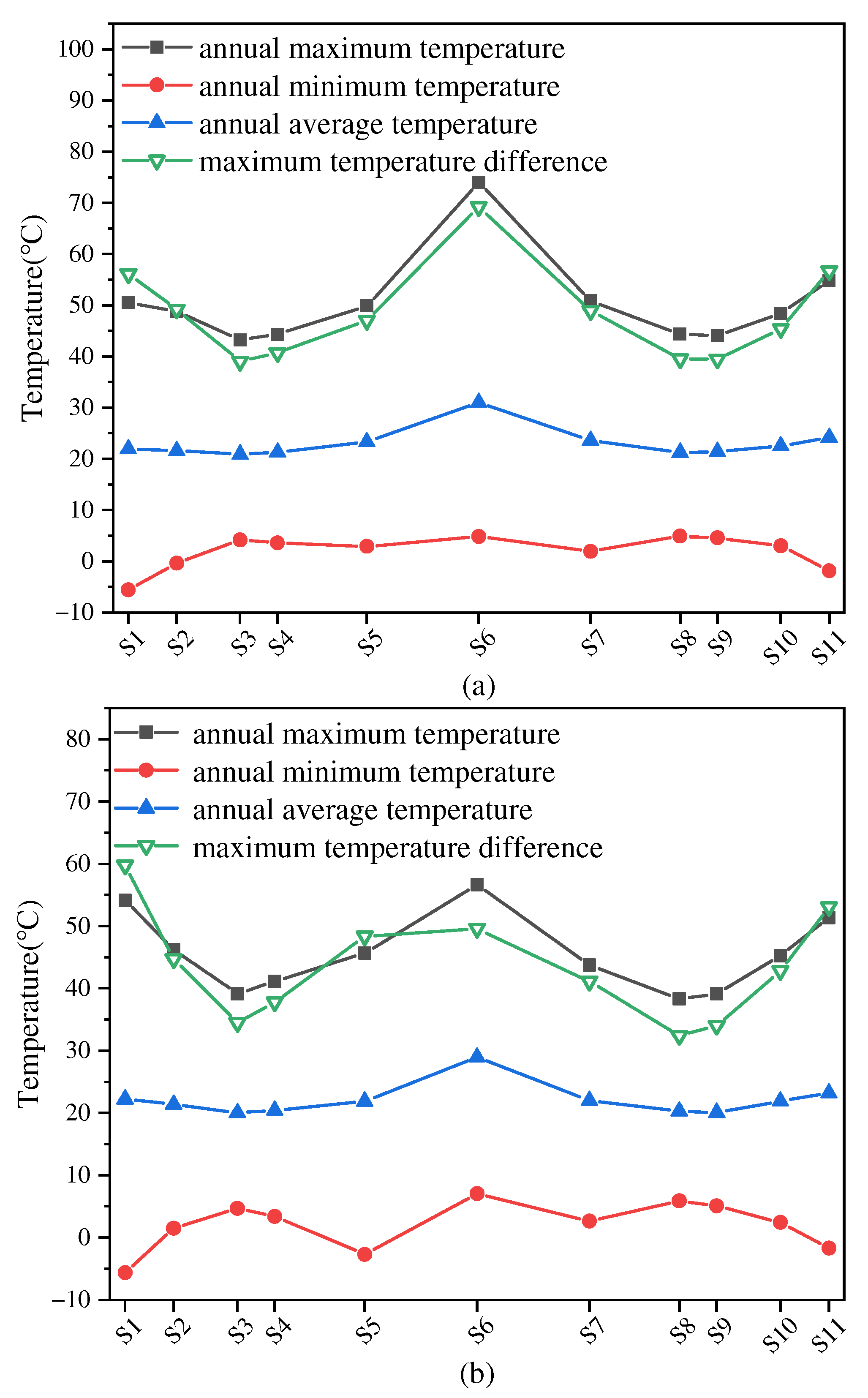
To further analyze the longitudinal gradient of the bridge girder surface temperature, the annual temperature and annual temperature difference were statistically analyzed by selecting one year of the temperature time history data from 11 measurement points (S1–S11) in the longitudinal direction. The statistical analyses included the following four aspects: annual maximum temperature, annual minimum temperature, annual average temperature and annual maximum temperature difference for each measurement point. The annual maximum temperature difference was the difference between the annual maximum temperature and the annual minimum temperature.
By taking the top and bottom measuring points, including T4 and T5; for instance, the annual temperature and statistical analyses along the longitudinal direction of the main bridge are shown in
Figure 9. An analysis of
Figure 9 shows that the distribution of the temperature field along the longitudinal direction was non-uniform. The average temperature was approximately symmetrical about the mid-span. On the other hand, the annual average and maximum temperature curves showed the same patterns: the temperature was highest in the middle of the span and lower near the bridge tower while also rising again from there to the side span. In addition, the variation trends of the annual maximum temperature difference were similar to that of the annual maximum temperature. Although there was some variation in the minimum temperature between the different measurement points, this variation was not very significant compared to the maximum temperature. In addition, compared to the bottom plate, the temperature variation range from the top plate was larger. Measured data show that many cities in China have experienced extremely high temperatures over recent years. For example, the maximum temperature in Chongqing reached 43 °C in 2022, and the temperature of the steel box girder, in this case, may show a peak. We will continue to follow up on the study.
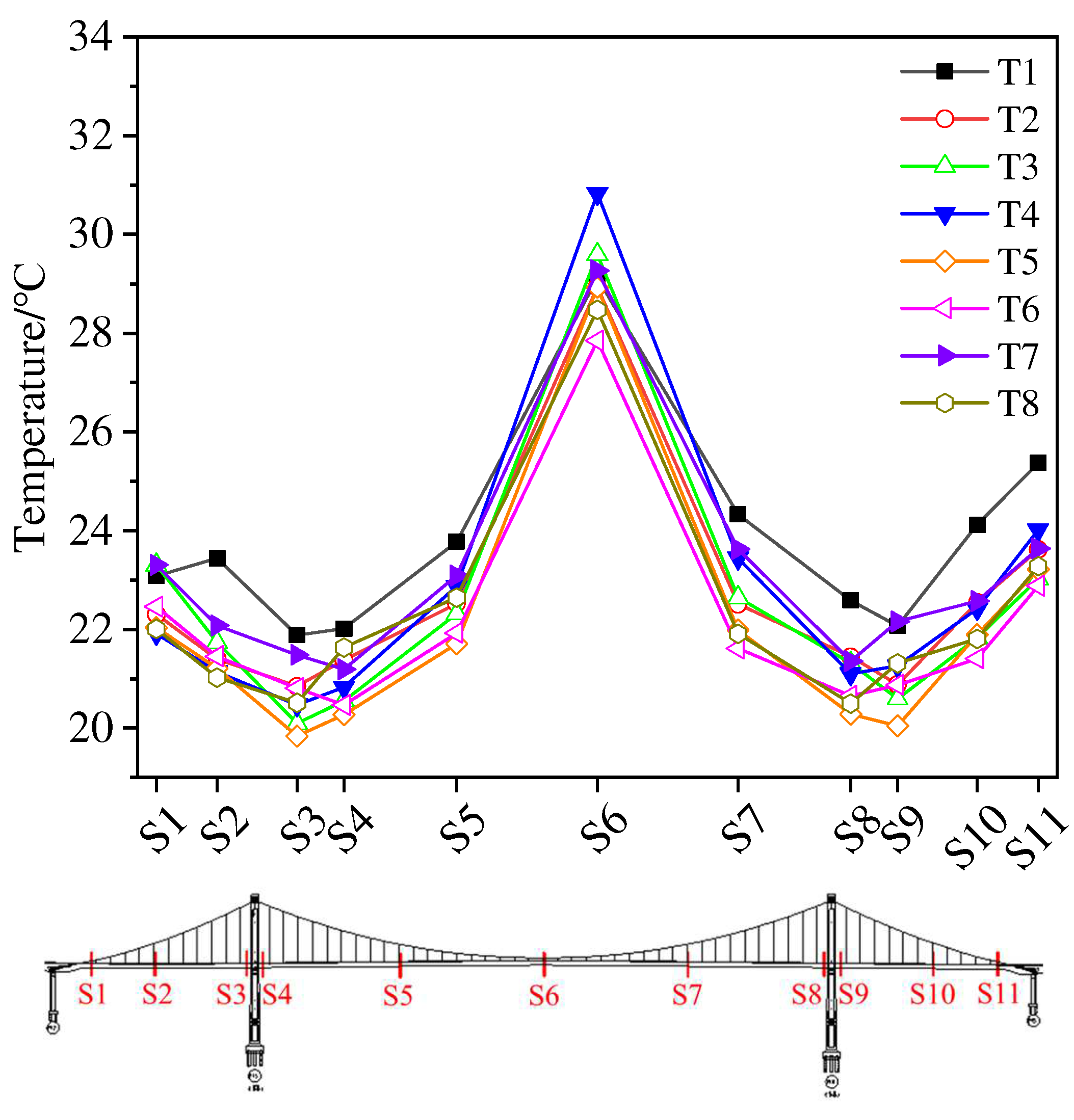
To further investigate the longitudinal temperature distribution pattern, the annual measured data for all eight temperature measuring points (T1~T8) in each section were statistically analyzed, and the annual average temperature of each measuring point is shown in
Figure 10. It can be seen that the surface temperature of the steel box girder had different distributions between the top and bottom plates, as well as the left and right sides of the mid-span. To clarify the distribution pattern, the polynomial fitting of the longitudinal temperature distribution curve was performed below.
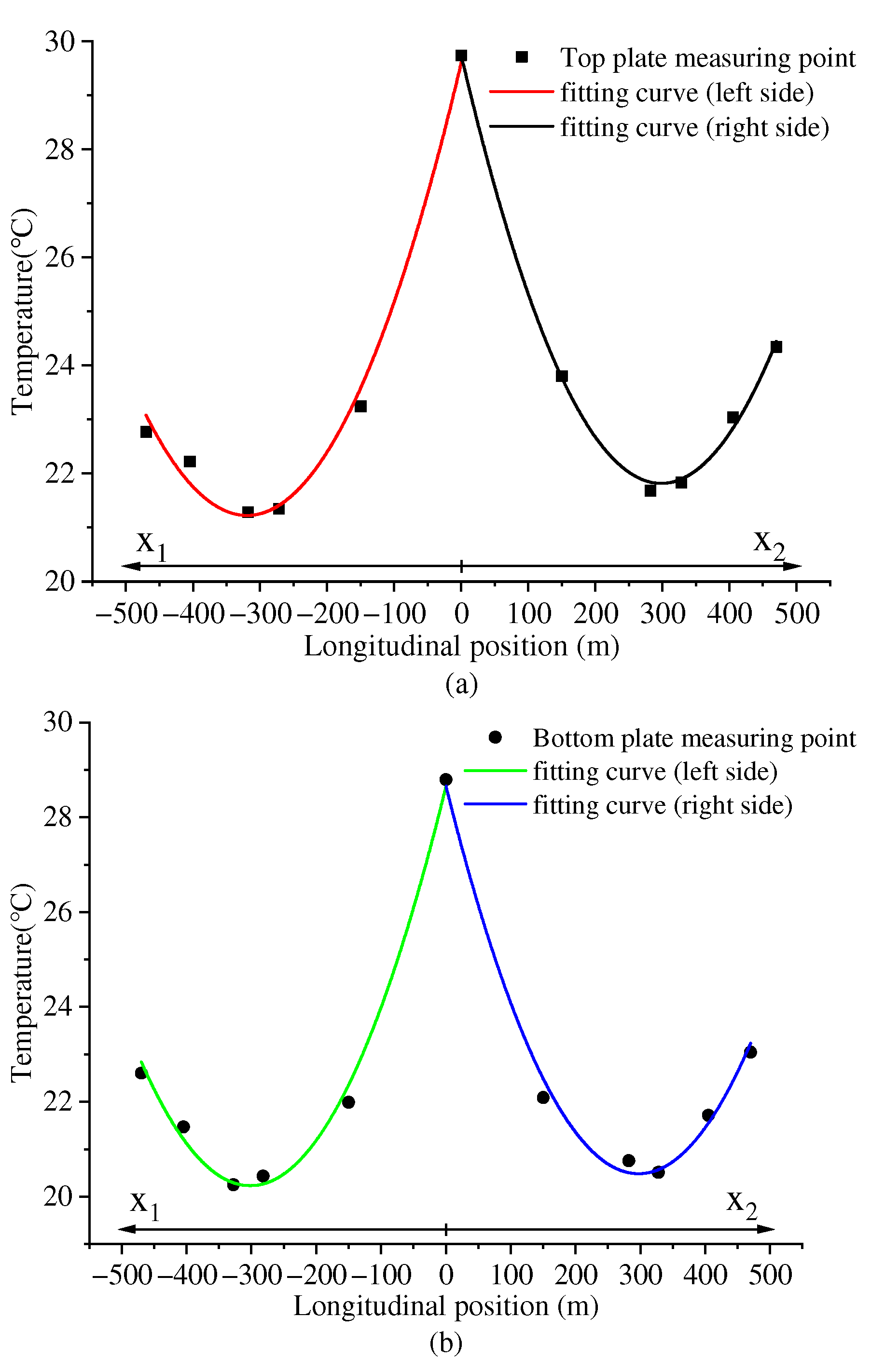
First, the measured temperature of the top and bottom plates was, respectively, time-averaged. Then, the average temperature values of different measuring points on the left and right sides of the mid-span (S6) were separately fitted using polynomial curves
, where
denoted the temperature value,
denoted the Longitudinal distance from the mid-span, and the three parameters of the equation were A, B, and C. In order to conveniently compare the fitted formulas, the horizontal axis on the left side was set as
and the horizontal axis on the right side was set as
. The fitting results are shown in
Figure 11. Meanwhile, the equations of the fitted curves are listed in
Table 2. The temperature values at any longitudinal location on the steel box girder could be subsequently estimated from these fitted curve equations. By referring to the practice of the specifications and other studies [
8,
26,
30,
33] on the horizontal and vertical temperature gradient patterns, in our future research work, we should incorporate data from other similar bridges to obtain the longitudinal temperature distribution patterns of large-span suspension bridges.
From the fitted curves and the fitting parameters, it could be seen that: (1) For the top plate temperature, the two fitting curves along the left and right spans had significantly different parameters, with higher temperatures on the right side than on the left side, possibly due to variations in geographic position and material properties. (2) For the bottom plate temperature, the two fitting curves along the left and right spans had very similar parameters, indicating that the temperature of the bottom plate was longitudinally distributed and symmetric along the mid-span.
4.2. Temperature Longitudinal Correlation Analysis
The analysis of statistical values, such as the annual mean and annual maximum temperatures, showed that there was a significant temperature gradient along the longitudinal direction of the bridge. To investigate the connection between surface temperatures at different longitudinal locations, correlation analysis was necessary. In order to evaluate the non-uniformity of the longitudinal temperature distribution, for each section measurement point (T1~T8), correlation analysis was performed with the same measurement points at other longitudinal positions, respectively. The position of S6 (mid-span) was taken as the reference point, where the correlation coefficient [
47] could be defined as:
where,
denoted the surface temperature of the steel box girder,
was the operator of covariance,
corresponded to time, and
and
represented different longitudinal measuring points.
Figure 12 shows the correlation analysis results and reveals that: (1) On the main span, the correlation coefficient decreased as the distance from S6 increased. This indicated that S6 had a greater effect on the temperature of S5 and S7 compared to S4 and S8. (2) The lowest correlation was found at the bridge tower. This is probably a result of the variability in the spatial distribution of cross-sections due to differences in the duration and intensity of the solar radiation received. The solar radiation at the bridge tower would be absorbed more by the tower, so the correlation coefficient of the S4 and S8 cross-sections was the lowest. (3) The sudden increase in the correlation coefficients of cross-sections S3 and S9 at the side span position indicated that solar radiation had a more dominant effect than the shading effect on the bridge tower. (4) The temperature correlation coefficient was generally higher on the right side of the mid-span than on the left side, meaning that the temperature was more uniform on the right side than on the left side. In addition, the upstream and downstream sides showed different temperature correlation characteristics. These differences may be related to the differences in bridge orientation, section form and material properties.
The longitudinal correlation analysis showed again that the longitudinal temperature distribution was non-uniform. These results were more comprehensive than previous studies with limited point comparisons. Therefore, using single-point measurement data to represent the temperature field may lead to overestimating or underestimating the temperature effect at different bridge spanwise locations. As a result, the temperature effects of large-span bridges could not be assessed accurately.
5. Mapping Longitudinal Temperature Variation Contours
5.1. Power Spectral Density
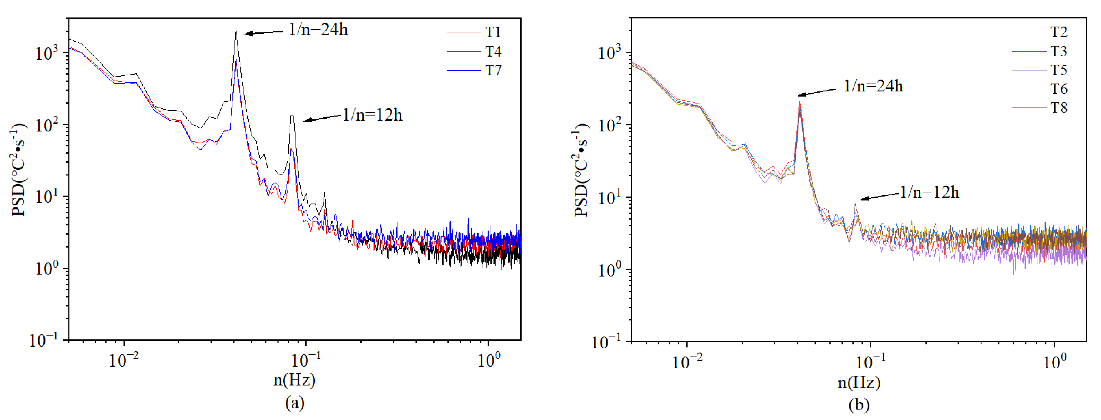
Power Spectral Densities (PSDs) refer to the spectral energy distribution per unit of time. PSDs focus on various features of the signal in the frequency domain, intending to extract useful signals in frequency domains that are drowned in noise. Based on Fourier transform, the PSDs of the annual temperatures of the girder surface temperature could be calculated. Taking a typical section S6 for an example, the results of the top and bottom plates are shown in
Figure 13.
There are two prominent peaks that can be observed in the PSD of
Figure 13. The period of the first peak was 24 h, which was identical to the daily period. The period of the second peak was 12 h, which was induced by the transmission from day to night. The results of PSD analysis show that the daily temperature could be considered a representative sample of the annual temperature. Moreover, the daily temperature could provide a more detailed view of the temperature change process compared to the annual temperature. Therefore, the temperature in one day can be selected to investigate the mechanisms and processes of longitudinal temperature gradients.
In addition, the PSD generally decreased with the increase in frequency and tended to become a horizontal line in the high-frequency region. The general decreasing trend resulted from a reduction in the high-frequency components of temperature. When this frequency was high enough, the temperature did not change in the corresponding short period. Thus, the PSD was almost horizontal in the high-frequency region. These results indicate that the surface temperature of the steel box girder was mainly controlled by low-frequency components, and the high-frequency effect was less affected.
5.2. Contours of Daily Temperature
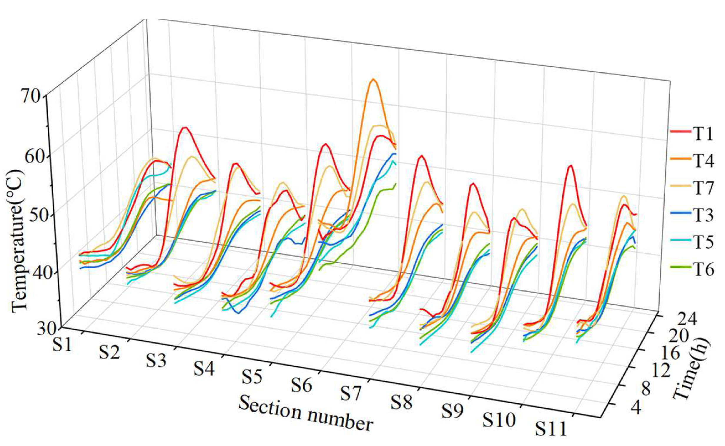
To further analyze the generation mechanisms and processes of the longitudinal temperature gradient, taking into account the apparent daily periodicity of the temperature data, the data for one day were selected for analysis. The following is an analysis of the longitudinal temperature distribution pattern based on daily temperature curves. A total of 11 longitudinal sections were selected, and three measurement points on each of the top and bottom surfaces were taken for analysis. To better observe their regularity, the hourly temperature was averaged to obtain the time history of the measured daily temperature curves, as shown in
Figure 14.
Figure 14 points out that, as summarized in the previous section, the temperature distribution along the longitudinal direction was always non-uniform. The temperature statistic values varied non-uniformly in spatial locations, and the temperature transients varied non-uniformly in space as well. Thus, the non-uniform longitudinal temperature gradient contained both spatial non-uniformity and temporal non-uniformity. Although previous studies have investigated the effect of temperature at different longitudinal locations on the temperature gradient of the cross-section through finite points, they have not investigated the mechanism of this non-uniform temperature field in depth.
Meanwhile, Sections S3, S4 and S8, S9 are, respectively, located on both sides of the east and west main towers. The amplitude of daily temperature variation in these cross-sections was smaller than that of other adjacent measurement points. This phenomenon is similar to the findings of
Figure 10 and
Figure 12. Additionally, this was mainly due to the shading effect of the main tower, which reduced the temperature of this section. In addition, the temperature of the mid-span S6 section was the highest because it was directly affected by solar radiation. By comparing the temperature-time histories of the top and bottom plates between different sections, it is found that there was a difference in the longitudinal temperature distribution between the top and bottom surfaces.
If the surface temperature of any position on the box girder could be obtained, the accuracy of the temperature effect analysis could be improved. Therefore,
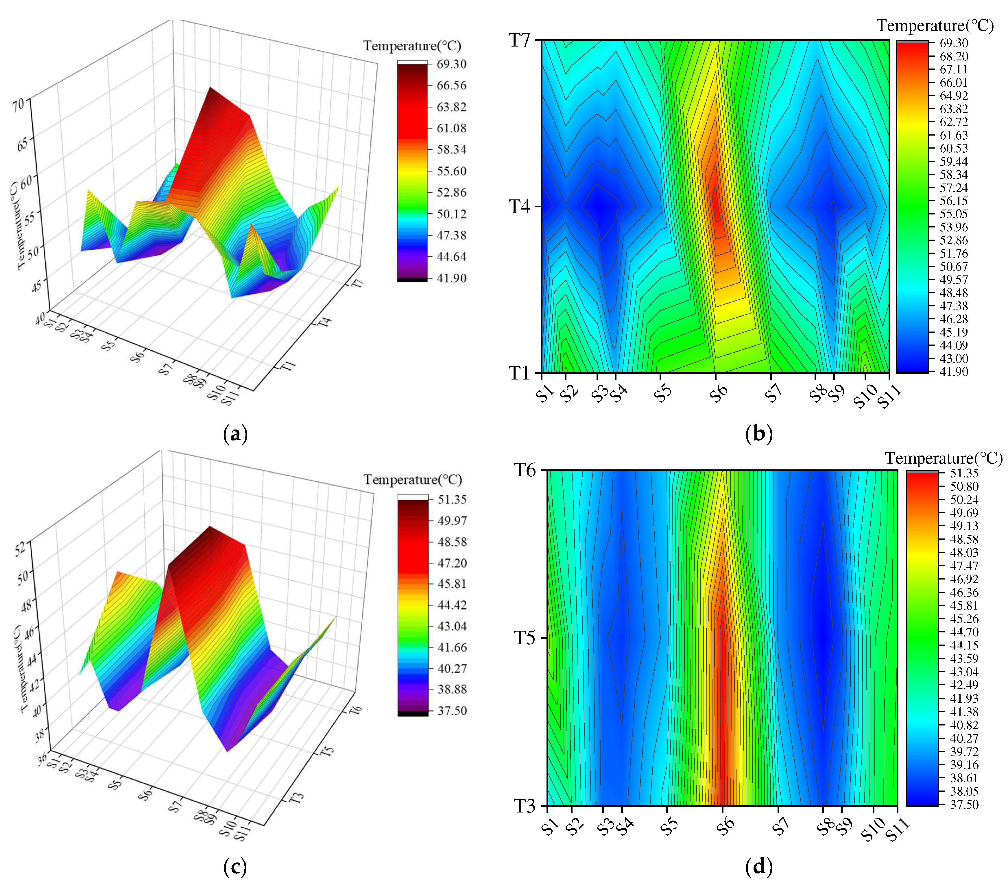
Figure 15 shows the daily temperature contour maps of the top and bottom plate temperatures, respectively. The example time instant was chosen at 17:00 because the girder surface temperature at that time was the highest value in one day, and the longitudinal temperature distribution of the steel box girder had obvious non-uniformity.
It can be seen from
Figure 15 that: (1) The longitudinal temperature contour on the top plate indicates that the high-temperature area slightly deviated to the right of the mid-span. This is because the bridge is east–west oriented, and the bridge deck on the right side of the mid-span was exposed to solar radiation for a longer time, so the temperature would be slightly higher than the bridge deck on the left side of the mid-span. (2) The longitudinal temperature distribution of the bottom plate was almost symmetrical about the mid-span because the bottom plate was not directly affected by solar radiation but was mainly affected by the environmental temperature. (3) The transverse temperature difference of the top plate was more obvious than that of the bottom plate because of solar radiation, and the temperature distribution had obvious three-dimensional spatial distribution characteristics.
After analyzing the temperature distribution characteristics on other days, we could also obtain a similar conclusion. The longitudinal distribution characteristics of daily and annual temperature were similar, while daily temperature also had a three-dimensional spatial distribution.
To summarize, the temperature of the long-span bridge structure was non-uniformly distributed not only in space but also in time. The non-uniformity of the longitudinal temperature distribution could be caused by the non-uniformity of the material and is also related to the environmental location where the measurement points are located. When performing temperature effect analysis, the temperature field of large-scale bridge structures is usually assumed to be a one-dimensional temperature field, which erases the longitudinal and transverse temperature gradients, resulting in large deviations between the calculated results and the real temperature field of the bridge. Further research into the effects of these factors on the longitudinal temperature distributions could be useful in the design stage of long-span bridges to effectively reduce the risk caused by the temperature effects. Therefore, during the refinement of the temperature effect analysis for long-span bridges, the longitudinal distribution of temperature non-uniformity needed to be considered.
6. Conclusions
This study investigated the longitudinal distribution characteristics of the box girder surface temperature on a long-span suspension bridge. The probability density statistics, statistical values, cross-correlations coefficients, power spectrum densities, and time-space contours are detailed and analyzed. The main findings are as follows:
(1) The annual temperature’s probability density curves at different longitudinal measuring points of the bridge all have bimodal characteristics, which could be fitted by the weighted sum of two normal distributions. This bimodal distribution was mainly caused by the transitions between different seasons.
(2) The statistical analyses show that the distribution of the girder surface temperature along the longitudinal direction was non-uniform. Moreover, the equations of the longitudinal distribution curves were obtained by polynomial fitting, and the distribution pattern was the highest in the mid-span, the lowest in the bridge tower, and increased along the side span. Therefore, the design phase should consider the non-uniform distribution of temperature.
(3) Using the correlation analysis between the temperature measured at the mid-span and other longitudinal sections, it was found that the correlation coefficient in the main span gradually decreased farther away from the mid-span section, with the lowest at the tower section. While in the side span, the correlation coefficient increased as the measurement points moved away from the tower. This revealed that the girder surface temperature was influenced by solar radiation and also the shedding effects of the tower.
(4) There were two prominent peaks in the frequency domain of the annual temperature, corresponding to the 24 h and 12 h time periods, respectively. This meant that the daily temperature could be considered a representative sample of the annual temperature.
(5) By comparing the daily time histories of temperature at different longitudinal sections, it was found that the temperature field was significantly three-dimensional and was not only non-uniformly distributed in space but also non-uniformly distributed in time.
(6) According to the time-space contour maps of temperature, we can gain insight into the underlying mechanisms of the generation of this non-uniformity distribution. Combined with the statistical analyses, the statistical values of the bridge temperature at any section could be obtained using the contour map.
In conclusion, the surface temperature of the steel box girder was non-uniformly distributed along the longitudinal direction of the bridge. Therefore, in analyzing the temperature effects, the traditional uniform-distribution assumption could lead to inestimable deviations from the real conditions. This work is helpful for a more accurate analysis of temperature effects on long-span bridges and can also provide a reference for the longitudinal distribution of temperature fields on other similar bridges.
Author Contributions
Conceptualization, W.M. and B.W.; Formal analysis, W.M. and B.W.; Methodology, W.M. and B.W.; Data curation, D.Q. and B.Z.; Validation, D.Q. and B.Z.; Investigation, D.Q. and X.Y.; Writing—original draft, W.M.; Writing—review and editing, B.W.; Project administration, B.W. and X.Y.; Funding acquisition, B.W. and X.Y. All authors have read and agreed to the published version of the manuscript.
Funding
This work was supported by the National Natural Science Foundation of China (Grant No. 51978111), Chongqing Technology Innovation and Application Development Special Key Project (Grant No. CSTB 2022TIAD-KPX0205), Chongqing Transportation Science and Technology Project (Grant No. 2022-01), Natural Science Foundation of Chongqing, China (Grant No. cstc2021jcyj-bshX0061), China Postdoctoral Science Foundation (Grant No. 2022MD713699), Special Funding of Chongqing Postdoctoral Research Project (Grant No. 2021XM1016) and Chongqing Zhongxian Science and Technology Plan Project (Grant No. zxkyxm202202) are greatly acknowledged.
Data Availability Statement
Data are available on request due to restrictions.
Conflicts of Interest
The authors declare no conflict of interest.
References
- Wang, J.F.; Zhang, J.T.; Xu, R.Q.; Yang, Z.X. Evaluation of Thermal Effects on Cable Forces of a Long-Span Prestressed Concrete Cable–Stayed Bridge. J. Perform. Constr. Facil. 2019, 33, 04019072. [Google Scholar] [CrossRef]
- Honarvar, E.; Sritharan, S.; Rouse, J.M.; Meeker, W.Q. Probabilistic Approach to Integrating Thermal Effects in Camber and Stress Analyses of Concrete Beams. J. Bridge Eng. 2020, 25, 04020010. [Google Scholar] [CrossRef]
- Zhou, Y.; Xia, Y.; Chen, B.; Fujino, Y. Analytical Solution to Temperature-Induced Deformation of Suspension Bridges. Mech. Syst. Signal Process. 2020, 139, 106568. [Google Scholar] [CrossRef]
- McClure, R.M.; West, H.H.; Hoffman, P.C. Observations from Tests on a Segmental Bridge. Transp. Res. Rec. 1984, 2, 60–67. [Google Scholar]
- Riding, K.A.; Poole, J.L.; Schindler, A.K.; Juenger, M.C.; Folliard, K.J. Temperature Boundary Condition Models for Concrete Bridge Members. ACI Mater. J. 2007, 104, 379–387. [Google Scholar]
- Tayşi, N.; Abid, S. Temperature Distributions and Variations in Concrete Box-Girder Bridges: Experimental and Finite Element Parametric Studies. Adv. Struct. Eng. 2015, 18, 469–486. [Google Scholar] [CrossRef]
- Li, S.; Xin, J.; Jiang, Y.; Wang, C.; Zhou, J.; Yang, X. Temperature-Induced Deflection Separation Based on Bridge Deflection Data Using the TVFEMD-PE-KLD Method. J. Civ. Struct. Health Monit. 2023, 13, 781–797. [Google Scholar] [CrossRef]
- Xue, J.; Lin, J.; Briseghella, B.; Tabatabai, H.; Chen, B. Solar Radiation Parameters for Assessing Temperature Distributions on Bridge Cross-Sections. Appl. Sci. 2018, 8, 627. [Google Scholar] [CrossRef]
- Honorio, T.; Bary, B.; Benboudjema, F. Evaluation of the Contribution of Boundary and Initial Conditions in the Chemo-Thermal Analysis of a Massive Concrete Structure. Eng. Struct. 2014, 80, 173–188. [Google Scholar] [CrossRef]
- Zhang, F.; Shen, J.; Liu, J. Effect of Encased Concrete on Section Temperature Gradient of Corrugated Steel Web Box Girder. Adv. Struct. Eng. 2021, 24, 2321–2335. [Google Scholar] [CrossRef]
- Zhou, L.; Xia, Y.; Brownjohn, J.M.W.; Koo, K.Y. Temperature Analysis of a Long-Span Suspension Bridge Based on Field Monitoring and Numerical Simulation. J. Bridge Eng. 2016, 21, 04015027. [Google Scholar] [CrossRef]
- Yang, L.I.U.; Hai-ping, Z.; Yang, D.; Nan, J.; Jian-ren, Z. Temperature Field Characteristic Research of Steel Box Girder for Suspension Bridge Based on Measured Data. China J. Highw. Transp. 2017, 30, 56. [Google Scholar]
- Shi, T.; Zheng, J.; Deng, N.; Chen, Z.; Guo, X.; Wang, S. Temperature Load Parameters and Thermal Effects of a Long-Span Concrete-Filled Steel Tube Arch Bridge in Tibet. Adv. Mater. Sci. Eng. 2020, 2020, 9710613. [Google Scholar] [CrossRef]
- Abid, S.R.; Tayşi, N.; Özakça, M. Experimental Analysis of Temperature Gradients in Concrete Box-Girders. Constr. Build. Mater. 2016, 106, 523–532. [Google Scholar] [CrossRef]
- Peiretti, H.C.; Parrotta, J.E.; Oregui, A.B.; Caldentey, A.P.; Fernandez, F.A. Experimental Study of Thermal Actions on a Solid Slab Concrete Deck Bridge and Comparison with Eurocode 1. J. Bridge Eng. 2014, 19, 04014041. [Google Scholar] [CrossRef]
- Hedegaard, B.D.; French, C.E.; Shield, C.K. Investigation of Thermal Gradient Effects in the I-35W St. Anthony Falls Bridge. J. Bridge Eng. 2013, 18, 890–900. [Google Scholar] [CrossRef]
- Lee, J.-H.; Kalkan, I. Analysis of Thermal Environmental Effects on Precast, Prestressed Concrete Bridge Girders: Temperature Differentials and Thermal Deformations. Adv. Struct. Eng. 2012, 15, 447–459. [Google Scholar] [CrossRef]
- Ding, Y.; Zhou, G.; Li, A.; Wang, G. Thermal Field Characteristic Analysis of Steel Box Girder Based on Long-Term Measurement Data. Int. J. Steel Struct. 2012, 12, 219–232. [Google Scholar] [CrossRef]
- Wang, G.; Ding, Y.; Wang, X.; Yan, X.; Zhang, Y. Long-Term Temperature Monitoring and Statistical Analysis on the Flat Steel-Box Girder of Sutong Bridge. J. Highway Transp. Res. Dev. 2014, 8, 63–68. [Google Scholar] [CrossRef]
- Zhang, C.; Liu, Y.; Liu, J.; Yuan, Z.; Zhang, G.; Ma, Z. Validation of Long-Term Temperature Simulations in a Steel-Concrete Composite Girder. Structures 2020, 27, 1962–1976. [Google Scholar] [CrossRef]
- Xia, Y.; Xu, Y.-L.; Wei, Z.-L.; Zhu, H.-P.; Zhou, X.-Q. Variation of Structural Vibration Characteristics versus Non-Uniform Temperature Distribution. Eng. Struct. 2011, 33, 146–153. [Google Scholar] [CrossRef]
- Xin, J.; Jiang, Y.; Zhou, J.; Peng, L.; Liu, S.; Tang, Q. Bridge Deformation Prediction Based on SHM Data Using Improved VMD and Conditional KDE. Eng. Struct. 2022, 261, 114285. [Google Scholar] [CrossRef]
- Zhang, H.; Li, H.; Zhou, J.; Tong, K.; Xia, R. A Multi-Dimensional Evaluation of Wire Breakage in Bridge Cable Based on Self-Magnetic Flux Leakage Signals. J. Magn. Magn. Mater. 2023, 566, 170321. [Google Scholar] [CrossRef]
- Zeng, Y.; He, H.; Qu, Y.; Sun, X.; Tan, H.; Zhou, J. Numerical Simulation of Fatigue Cracking of Diaphragm Notch in Orthotropic Steel Deck Model. Materials 2023, 16, 467. [Google Scholar] [CrossRef] [PubMed]
- Zeng, Y.; Qiu, Z.; Yang, C.; Haozheng, S.; Xiang, Z.; Zhou, J. Fatigue Experimental Study on Full-Scale Large Sectional Model of Orthotropic Steel Deck of Urban Rail Bridge. Adv. Mech. Eng. 2023, 15, 16878132231155272. [Google Scholar] [CrossRef]
- AASHTO. AASHTO LRFD Bridge Design Specifications; American Association of State Highway and Transportation Officials: Washington, DC, USA, 2012. [Google Scholar]
- BS 5400: Part 2; Concrete and Composite Bridges. Specification for Loads. British Standard Institution: London, UK, 1978.
- EN 1991-1; Eurocode 1—Actions on Structures—Part 1-5: General Actions—Thermal Actions. CEN (European Committee for Standardization): Brussels, Belgium, 2004.
- AS5100. 2-2004; Bridge Design—Part 2. Design Load. Standards Australia: Sydney, NSW, Australia, 2004.
- JTG D60-2015; General Specifications for Design of Highway Bridges and Culverts. China Communications Press: Beijing, China, 2015.
- Niu, Y.; Wang, Y.; Tang, Y. Analysis of Temperature-Induced Deformation and Stress Distribution of Long-Span Concrete Truss Combination Arch Bridge Based on Bridge Health Monitoring Data and Finite Element Simulation. Int. J. Distrib. Sens. Netw. 2020, 16, 1550147720945205. [Google Scholar] [CrossRef]
- Taeb, A.; Ooi, P.S. Comparison of Field Behavior with Results from Numerical Analysis of a Geosynthetic Reinforced Soil Integrated Bridge System Subjected to Thermal Effects. Transp. Res. Rec. 2020, 2674, 294–306. [Google Scholar] [CrossRef]
- Wang, D.; Liu, Y.; Liu, Y. 3D Temperature Gradient Effect on a Steel-Concrete Composite Deck in a Suspension Bridge with Field Monitoring Data. Struct. Control. Health Monit. 2018, 25, e2179. [Google Scholar] [CrossRef]
- Jiang, Y.; Hui, Y.; Wang, Y.; Peng, L.; Huang, G.; Liu, S. A Novel Eigenvalue-Based Iterative Simulation Method for Multi-Dimensional Homogeneous Non-Gaussian Stochastic Vector Fields. Struct. Saf. 2023, 100, 102290. [Google Scholar] [CrossRef]
- Abid, S.R. Three-Dimensional Finite Element Temperature Gradient Analysis in Concrete Bridge Girders Subjected to Environmental Thermal Loads. Cogent Eng. 2018, 5, 1447223. [Google Scholar] [CrossRef]
- Hu, J.; Wang, L.; Song, X.; Sun, Z.; Cui, J.; Huang, G. Field Monitoring and Response Characteristics of Longitudinal Movements of Expansion Joints in Long-Span Suspension Bridges. Measurement 2020, 162, 107933. [Google Scholar] [CrossRef]
- Gu, B.; Zhou, F.Y.; Gao, W.; Xie, F.Z.; Lei, L.H. Temperature Gradient and Its Effect on Long-Span Prestressed Concrete Box Girder Bridge. Adv. Civ. Eng. 2020, 2020, 5956264. [Google Scholar] [CrossRef]
- Liu, J.; Liu, Y.; Zhang, C.; Zhao, Q.; Lyu, Y.; Jiang, L. Temperature Action and Effect of Concrete-Filled Steel Tubular Bridges: A Review. J. Traffic Transp. Eng. 2020, 7, 174–191. [Google Scholar] [CrossRef]
- Xin, J.; Zhou, C.; Jiang, Y.; Tang, Q.; Yang, X.; Zhou, J. A Signal Recovery Method for Bridge Monitoring System Using TVFEMD and Encoder-Decoder Aided LSTM. Measurement 2023, 112797. [Google Scholar] [CrossRef]
- Morgese, M.; Wang, C.; Ying, Y.; Taylor, T.; Ansari, F. Stress–Strain Response of Optical Fibers in Direct Tension. J. Eng. Mech. 2023, 149, 04023037. [Google Scholar] [CrossRef]
- Tang, Q.; Xin, J.; Jiang, Y.; Zhou, J.; Li, S.; Chen, Z. Novel Identification Technique of Moving Loads Using the Random Response Power Spectral Density and Deep Transfer Learning. Measurement 2022, 195, 111120. [Google Scholar] [CrossRef]
- Wang, C.; Ansari, F.; Wu, B.; Li, S.; Morgese, M.; Zhou, J. LSTM Approach for Condition Assessment of Suspension Bridges Based on Time-Series Deflection and Temperature Data. Adv. Struct. Eng. 2022, 25, 3450–3463. [Google Scholar] [CrossRef]
- Zhang, H.; Ma, X.; Jiang, H.; Tong, K.; Zheng, Y.; Zhou, J. Grading Evaluation of Overall Corrosion Degree of Corroded RC Beams via SMFL Technique. Struct. Control. Health Monit. 2023, 2023, 6672832. [Google Scholar] [CrossRef]
- Wu, B.; Zhou, J.; Li, S.; Xin, J.; Zhang, H.; Yang, X. Combining Active and Passive Wind Tunnel Tests to Determine the Aerodynamic Admittances of a Bridge Girder. J. Wind. Eng. Ind. Aerodyn. 2022, 231, 105180. [Google Scholar] [CrossRef]
- Wu, F.; Zhou, J.; Xin, J.; Zhang, H.; Zhao, N.; Yang, X. Wind Damage Estimation of Roof Sheathing Panels Considering Directionality: Influences of Both Correlations of Directional Wind Speeds and Multiple Response Coefficients in Each Direction. J. Wind. Eng. Ind. Aerodyn. 2023, 236, 105396. [Google Scholar] [CrossRef]
- Tao, T.; He, J.; Wang, H.; Zhao, K. Efficient Simulation of Non-Stationary Non-Homogeneous Wind Field: Fusion of Multi-Dimensional Interpolation and NUFFT. J. Wind. Eng. Ind. Aerodyn. 2023, 236, 105394. [Google Scholar] [CrossRef]
- Li, H.; Zhang, L.; Wu, B.; Yang, Y.; Xiao, Z. Investigation of the 2D Aerodynamic Admittances of a Closed-Box Girder in Sinusoidal Flow Field. KSCE J. Civ. Eng. 2022, 26, 1267–1281. [Google Scholar] [CrossRef]
Figure 1.
Egongyan rail bridge.
Figure 1.
Egongyan rail bridge.
Figure 2.
Elevation layout of the main bridge (Unit: m).
Figure 2.
Elevation layout of the main bridge (Unit: m).
Figure 3.
The layout of the temperature monitoring points. (S: Section number; T: Number of temperature sensors arranged on each section).
Figure 3.
The layout of the temperature monitoring points. (S: Section number; T: Number of temperature sensors arranged on each section).
Figure 4.
JMZX-212HAT surface intelligent digital string strain gauge.
Figure 4.
JMZX-212HAT surface intelligent digital string strain gauge.
Figure 5.
Annual time-history of the girder surface temperature. (S-T: Sensor number T The section number S).
Figure 5.
Annual time-history of the girder surface temperature. (S-T: Sensor number T The section number S).
Figure 6.
Fitting of the PDFs of temperature at S2-T4 using different models: (a) Gaussian distribution model; (b) Superposition of two normal distribution models.
Figure 6.
Fitting of the PDFs of temperature at S2-T4 using different models: (a) Gaussian distribution model; (b) Superposition of two normal distribution models.
Figure 7.
Probability density histograms and the fitting curves of S2-T4, S6-T4 and S10-T4.
Figure 7.
Probability density histograms and the fitting curves of S2-T4, S6-T4 and S10-T4.
Figure 8.
Fitted PDFs of the girder surface temperatures at different longitudinal sections. (a) Top plate measuring points; (b) Bottom plate measuring points.
Figure 8.
Fitted PDFs of the girder surface temperatures at different longitudinal sections. (a) Top plate measuring points; (b) Bottom plate measuring points.
Figure 9.
Distribution of annual temperature statistic values along the longitudinal direction. (a) Top plate measuring points T4; (b) Bottom plate measuring points T5.
Figure 9.
Distribution of annual temperature statistic values along the longitudinal direction. (a) Top plate measuring points T4; (b) Bottom plate measuring points T5.
Figure 10.
Longitudinal distributions of annual average temperature.
Figure 10.
Longitudinal distributions of annual average temperature.
Figure 11.
Fitting curves of the temperature’s longitudinal distribution (a) Top plate; (b) Bottom plate.
Figure 11.
Fitting curves of the temperature’s longitudinal distribution (a) Top plate; (b) Bottom plate.
Figure 12.
Correlation analysis of the measurement points in the mid-span section with those in other locations.
Figure 12.
Correlation analysis of the measurement points in the mid-span section with those in other locations.
Figure 13.
The PSD of the measured annual temperature. (a) Top plate measurement points; (b) Bottom plate measurement points.
Figure 13.
The PSD of the measured annual temperature. (a) Top plate measurement points; (b) Bottom plate measurement points.
Figure 14.
Daily temperature-time histories for different measuring points at 11 sections.
Figure 14.
Daily temperature-time histories for different measuring points at 11 sections.
Figure 15.
Contour maps of measured temperature at 17:00. (a) Top plate temperature contours; (b) Projection of (a); (c) Bottom plate temperature contours; (d) Projection of (c).
Figure 15.
Contour maps of measured temperature at 17:00. (a) Top plate temperature contours; (b) Projection of (a); (c) Bottom plate temperature contours; (d) Projection of (c).
Table 1.
Estimated fitting parameters for the probability density models of typical measuring points.
Table 1.
Estimated fitting parameters for the probability density models of typical measuring points.
Measuring
Points | Fitting Parameters |
|---|
| | | | |
|---|
| S2-T4 | 0.9360 | 8.9207 | 1.8087 | 21.8373 | 9.8373 |
| S6-T4 | 0.9437 | 11.6900 | 2.3217 | 30.1064 | 16.2538 |
| S10-T4 | 0.9209 | 8.9665 | 1.6595 | 23.0285 | 11.1745 |
| S2-T5 | 0.9486 | 9.1765 | 1.6817 | 21.7870 | 10.6727 |
| S6-T5 | 0.9301 | 9.9613 | 2.2033 | 29.4177 | 16.9026 |
| S10-T5 | 0.9278 | 9.0896 | 1.6930 | 22.6721 | 11.1846 |
Table 2.
Longitudinal distribution of temperature fitting equation.
Table 2.
Longitudinal distribution of temperature fitting equation.
| Position | Fitted Curves Equation |
| Left side of the mid-span (top plate) | |
| Right side of the mid-span (bottom plate) | |
| Left side of the mid-span (top plate) | |
| Right side of the mid-span (bottom plate) | |
| Disclaimer/Publisher’s Note: The statements, opinions and data contained in all publications are solely those of the individual author(s) and contributor(s) and not of MDPI and/or the editor(s). MDPI and/or the editor(s) disclaim responsibility for any injury to people or property resulting from any ideas, methods, instructions or products referred to in the content. |
© 2023 by the authors. Licensee MDPI, Basel, Switzerland. This article is an open access article distributed under the terms and conditions of the Creative Commons Attribution (CC BY) license (https://creativecommons.org/licenses/by/4.0/).


