Research on Buffer Calculation Model of Critical Chain Based on Adjacency Information Entropy

Abstract

In project network planning, the correlation complexity of the processes is not only related to the immediately preceding and following processes, but also closely related to indirect adjacent processes. In the existing relevant studies, many scholars have considered the influence of direct adjacent processes but ignored the influence of indirect adjacent processes. In addition, the three-point time estimation method and Monte Carlo simulation are mostly used in the current research for the estimation of process duration, while less research exists on the estimation of process optimal duration under multi-objective constraints. Therefore, this paper proposes a buffer calculation model of critical chain based on adjacency information entropy. This methodology provides comprehensive consideration of the relationship between cost, quality, safety, environment and process duration, the influence of process’s resource demand intensity, resource constraints and process duration on the buffer size, the influence of the relay potential of mutual cooperation and cross construction between processes, as well as the influence of adjacent complexity of processes on the project construction schedule. The calculation example analysis shows that this method can improve the accuracy of the calculation of process safety time, reduce the influence of the complexity of process adjacency correlation on the project construction schedule, reasonably control the buffer size, and effectively shorten the planned project duration.

1. Introduction

Schedule, quality and cost are the three main management objectives in the field of project management. Schedule management, the core part of project management, is also the economic standard to measure the size of a construction project’s comprehensive management ability, and has a certain influence on the construction project’s duration, quality, cost and safety goals [1,2]. Critical chain, an emerging project schedule management technique, has received close attention from domestic and foreign scholars, and is the focus of research and a hot spot at the practical level in the current stage of project schedule management.

The critical chain was first introduced by Dr. Goldratt in his published management book, “The Critical Chain”. The core idea is to derive a work chain that constrains the duration by considering resource conflicts based on the traditional critical path. It also aggregates the safety time based on the risk aggregation principle and sets buffers centrally to counteract and absorb the negative impact of uncertainties during project construction to ensure the project’s timely completion. The project buffer is set at the end of the critical chain to absorb the uncertainty of all activities. The import buffer is set at the end of the non-critical chain to absorb the influence of process uncertainty on the critical chain [3].

The determination of critical chain buffer is the core of critical chain project management. Reasonable setting of buffer location and size can effectively eliminate the schedule risk that may arise due to various uncertain risk factors. It also helps to shorten the project duration, realize the interconnection of various objectives in the project management process, and improve the project management quality. By improving the calculation method of critical chain buffer size, we can ensure the efficient implementation of the project and provide reference for project management [4].

For the calculation of critical chain buffer size, many domestic and foreign scholars have conducted related research. Goldratt [3] proposed the concept of buffer along with the cut-and-paste method to determine the buffer. Herroelen and Leus [5,6] argued that the cut-and-paste method is relatively simple and suitable for calculating critical chain buffer for smaller scale projects, but stated larger projects with this calculation method would have an oversized buffer. Newbold [7] considered the probability of project completion and used the central limit theorem to propose the root variance method to calculate the buffer size. However, the shortcoming is that this method determines the buffer based on the independence of activity duration. Later, in view of the limitations of these two basic methods, many scholars have made various improvements to the calculation method of critical chain buffer size by comprehensively considering various risk factors affecting project progress. The existing research results are divided into three categories.

The first is the method based on project attributes. This method is to improve the root variance method by measuring the risk factors affecting the construction schedule in order to adjust the buffer setting. Tukel et al. [8] proposed a buffer calculation method considering resource tension and network complexity and the impact of the project’s own factors on buffer determination, which generated a new direction for buffer determination research. Chu [9] proposed a calculation method to adjust the buffer by comprehensively measuring the influencing factors such as project material tension, network composition complexity, and decision-maker risk preference, so that no matter how many processes are on the link, the buffer can be appropriate. Yang et al. [10] studied the plan buffer settings of critical chain by considering the three attributes related to specific projects, namely the number of processes, the uncertainty of processes’ execution time and the flexibility of commencement. Liu et al. [11] used factor analysis to extract 21 factors influencing the buffer setting of the project, and established a model for calculating the comprehensive weight of the process based on the weight of the influencing factors and their degree of influence on different processes. Hu et al. [12] proposed the addition of the remaining buffer of the non-critical chain to the modified model of project buffer, thereby reducing the influence of the non-critical chain on project duration. Paprocka and Czuwaj [13] proposed a method to estimate the size of the resource buffer and select the location of the resource buffer based on probability theory. Ghoddousi et al. [14] proposed a method of multi-attribute buffer size, which can generate stable project plans at low cost. Nie et al. [15] proposed a buffer size calculation method considering the influence of multi-resource constraints and relay potential, which can effectively shorten the project planning duration and reduce the project risk.

The second category is the assessment method based on fuzzy theory. Due to the uncertainty of project risk, fuzzy theory is frequently used for critical chain buffer calculation. Zhang et al. [16] measured the uncertainty risk of the process according to the ladder fuzzy number and determined an optimized buffer calculation method combined with resource tension and network complexity. Zohrehvandi et al. [17,18] introduced the Fuzzy Overlapping Buffer Management Algorithm to determine the size of the project buffer and dynamically control the consumption of the buffer. Marek and Katarzyna [19] applied normal distribution functions and fuzzy number theory to calculate the buffer size, which increased the chances of project execution. Lin et al. [20] quantified the uncertainty of each process based on the entropy weight method, and obtained the uncertainty coefficient of each process. Liu et al. [21] proposed a buffer size adjustment method which reflects the complexity of engineering schedule networks by structural entropy, which has good accuracy and effectiveness. Zhang et al. [22,23] proposed a critical chain buffer determination algorithm based on the entropy weight method. The entropy weight method was used to evaluate the uncertainty of the project and the fuzzy method was used to determine the dispersion degree and calculate the project buffer, which effectively improved the buffer management efficiency and optimized the buffer estimation accuracy. Liu et al. [24] developed an improved multi-criteria decision-making model to calculate the ‘green degree of ships’ concept to evaluate different alternatives based on a novel hybrid method, namely the group fuzzy entropy and cloud technique for order of preference by similarity to ideal solution theory. Wang et al. [25] first developed a hybrid multi-attribute decision making method, integrating regret theory and the entropy weighting method to measure the environmental and social sustainability of a disassembly by establishing an eight-criterion evaluation system of schemes.

The third category is based on project scheduling theory. The correct project scheduling can effectively predict the project progress and take effective response measures against unplanned changes to ensure the normal implementation and completion of the project. Long and Ohsato [26] proposed a fuzzy critical chain method under resource constraints and uncertainties, which provides an accurate schedule of project actual progress. Liu et al. [27] designed a heuristic algorithm based on priority rules under the resource-constrained project scheduling theory, while considering the free time of activities under resource constraints. Peng et al. [28] designed and implemented a new proactive–reactive integrated solution method based on the critical chain method to generate a robust and reliable baseline schedule for the resource constrained project scheduling problem of class under uncertainty.

From the above research, it can be seen that calculating buffer is becoming more scientific, the factors considered are gradually deepened, and a variety of improved buffer size calculation methods are proposed. However, there are still the following limitations: ① Process duration estimation is the basis of buffer estimation. The rationality and accuracy of process duration estimation directly affect the accuracy of buffer setting. For the estimation of process duration, most of the current studies are based on the three-point time estimation method and Monte Carlo simulation, and there are few studies using the impact of multi-objective constraints on the estimation of process duration. ② In current project network planning studies, only the correlation complexity of a process and its immediately preceding and following processes is considered. The correlation complexity of process is also closely related to its indirect adjacent processes and their impact is lost in these studies.

In view of the inadequacy of the existing critical chain buffer calculation methods, the following work has been done in this article: ① Considering the relationship between cost, quality, safety, environment, and process duration, respectively, to calculate the optimal process duration, thus improving the rationality of process safety time estimation. ② By considering the relationship between the process and its direct and indirect adjacent processes, the importance of the process is measured by using the adjacency information entropy in the project network plan. Its advantage is that we not only consider the complexity of the direct adjacent process of the process, but also integrate the influence of the indirect adjacent process. Because the algorithm only uses the local attributes of the process, its complexity is low.

Based on the above considerations, this article proposes a critical chain buffer calculation model based on adjacency information entropy. The optimal duration of the process under the multi-objective constraints of cost, quality, safety, and environment is comprehensively considered to improve the rationality of the process duration and safety time estimation. At the same time, the adjacency information entropy is used to measure the importance of different processes in the project network plan, and the buffer size of the critical chain is reasonably “added” or “reduced”, which is conducive to the smooth progress of project management and avoids the mutual disconnection of various objectives in the process of project management.

The article is organized as follows. In Section 2, we will provide the calculation methods of buffer size based on buffer influencing factors. In Section 3, we will introduce the calculation methods of various buffers of critical chain. In Section 4, the critical chain buffer calculation method in this article is applied to the project case, and the calculation results are compared and analyzed with other methods. Overall conclusions are outlined in Section 5.

2. Calculation Method for Influencing Factors of Buffer Size

In this section, we will provide the calculation methods for the influencing factors of multi-objective constraints, multi-resource constraints, process relay potential, and process adjacency information entropy on the buffer size.

2.1. A Method to Calculate the Influence of Multi-Objective Constraints on Buffer Size

Cost, quality, safety, environment, and project duration are the main contents of project management objective control; they are interdependent and mutually influential with obvious nonlinear relationships. Therefore, it is necessary to control the cost, quality, safety, environment, and process duration in a comprehensive and balanced way to improve the accuracy of the risk calculation method of process duration [29,30]. The Three-time Estimate method was used to estimate the most pessimistic, likely and optimistic durations of each process of the project. According to the results estimated by the Three-time Estimate method, the Crystal Ball software is used for simulation. The confidence levels of 25%, 50% and 95% correspond to the shortest duration T_ia, the average duration T_im and the longest duration T_ib of process i, respectively [31,32,33].

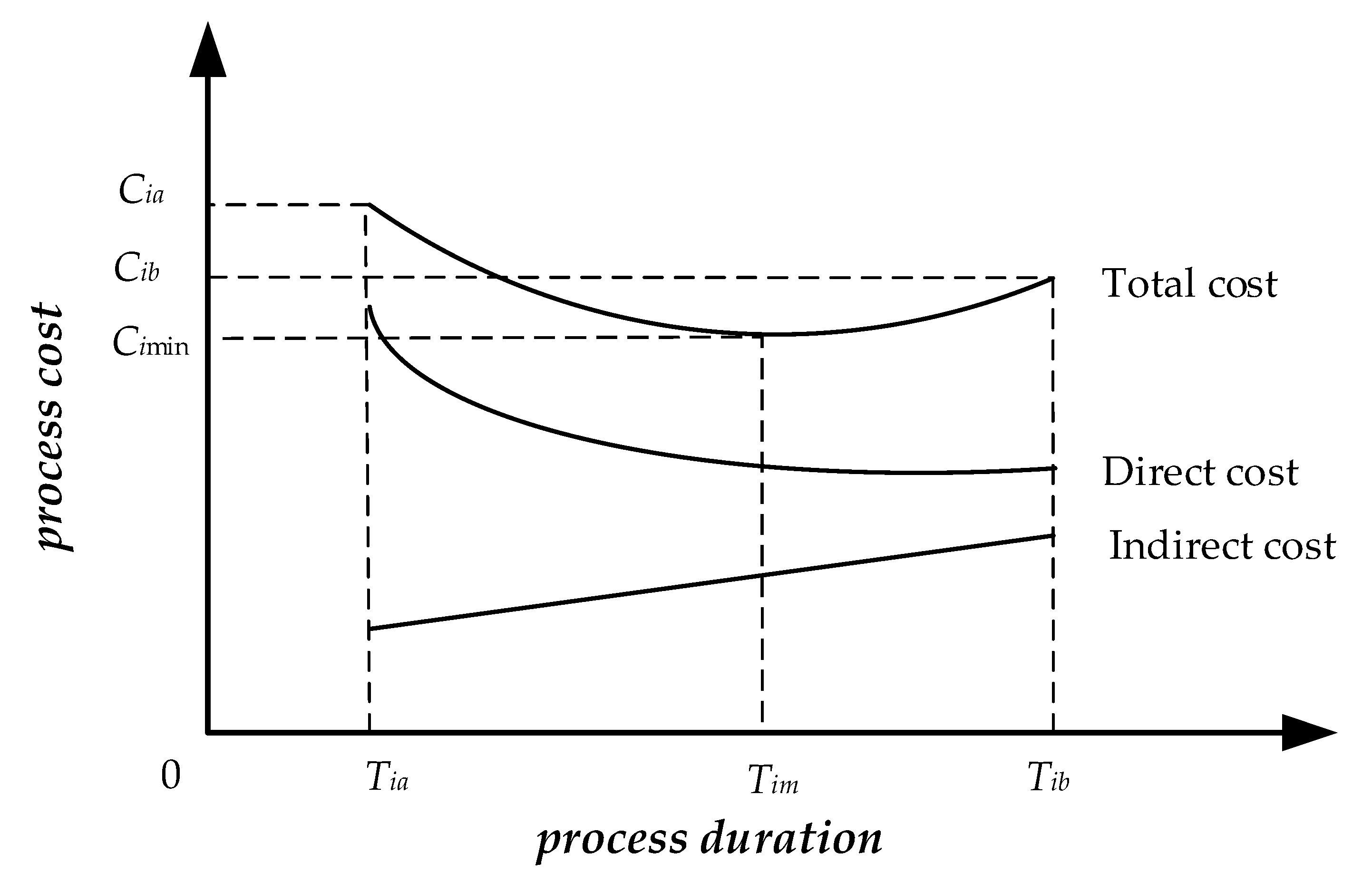
2.1.1. Cost-Time Model

The total cost of a process is composed of direct cost and indirect cost. The direct cost is quadratically related to the process duration, and the indirect cost is positively related to the process duration. The relationship between process cost and process duration is shown in Figure 1 [34,35,36].

The relationship model between total process cost and process duration is:

$$C_i={\rho }_i{(T_i-a_i)}^2+\delta T_i+b_i$$

(1)

$${\rho }_i=\frac{C_{ia}-C_{i\min }}{{(T_{ia}-T_{im})}^2}$$

(2)

$$a_i=T_{im}+\frac{\delta {(T_{ia}-T_{im})}^2}{2(C_{ia}-C_{i\min })}$$

(3)

$$b_i=C_{i\min }-\delta T_{im}-\frac{{\delta }^2{(T_{ia}-T_{im})}^2}{4(C_{ia}-C_{i\min })}$$

(4)

where C_i is the total cost corresponding to process i under the duration T_i; δ is the indirect cost rate; C_{i min} is the minimum total cost corresponding to process i under the average duration T_im; C_ia is the total cost corresponding to process i under the minimum duration T_ia; and C_ib is the total cost corresponding to process i under the maximum duration T_ib, a_i is the duration corresponding to the minimum direct cost of process i, and b_i is the minimum direct cost of process i.

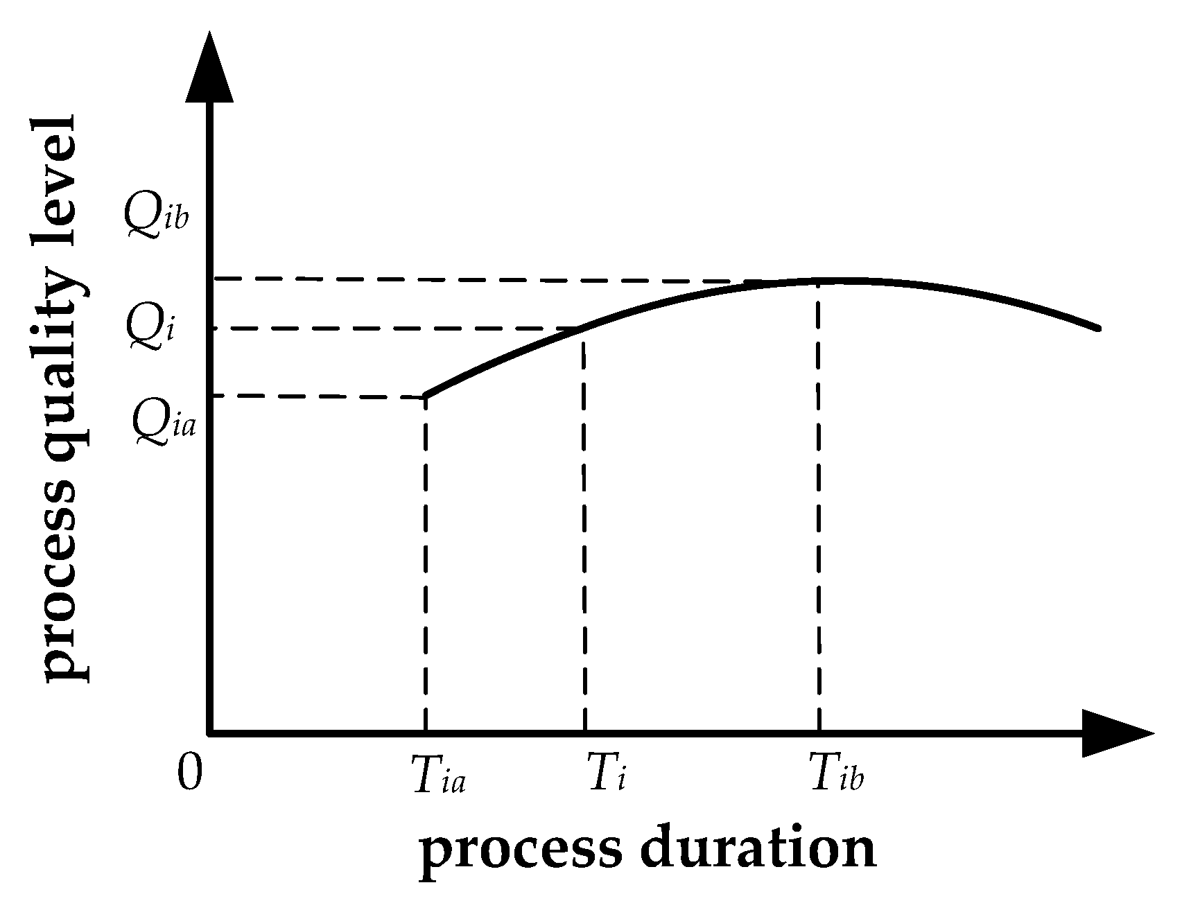
2.1.2. Quality-Time Model

According to actual engineering practice, we assume that the process quality level and duration have a certain relationship. When the process is completed in the shortest time, there are risks such as the reasonable technical interval is omitted, the construction is not standardized, the process is rough, eventually affecting the quality level of the process. The process quality level will increase with an increase of duration, but when the process duration increases to a certain value, the process quality will not rise linearly with time, but will slow down or even decline due to the decline of workers’ enthusiasm and the bottleneck of the process itself [37,38]. The relationship between process quality level and process duration is shown in Figure 2.

The relationship model between process quality level and process duration is:

$$Q_i=\ln (g_i{T}_i+f_i)$$

(5)

$$g_i=(e^{Q_{ib}}-e^{Q_{ia}})/(T_{ib}-T_{ia})$$

(6)

$$f_i=(e^{Q_{ia}}{T}_{ib}-e^{Q_{ib}}{T}_{ia})/(T_{ib}-T_{ia})$$

(7)

where Q_i is the quality level corresponding to process i under the duration T_i; Q_ib is the highest quality level corresponding to process i under the longest duration T_ib; and Q_ia is the lowest quality level corresponding to process i under the shortest duration T_ia. g_i is the growth rate of process quality level with duration, and f_i is the adjustment coefficient of the relationship between process quality level and duration.

2.1.3. Safety-Time Model

The relationship model between process safety level and process duration is:

$$S_i={\theta }_i(1-P_i)={\theta }_i[1-P_{io}(1-\Delta P_{io})]$$

(8)

$${\theta }_i=\left\{\begin{array}{ccc}\frac{T_i}{T_{im}}\hfill & \hfill ,\hfill & \hfill T_i < T_{im}\hfill \\ 1\hfill & \hfill ,\hfill & \hfill T_i \ge T_{im}\hfill \end{array}\right.$$

(9)

$$\Delta P_{io}=\Delta P_{io\min }+(\Delta P_{io\max }-\Delta P_{io\min })\frac{C_i-C_{i\min }}{C_{i\max }-C_{i\min }}$$

(10)

where S_i is the safety level of process i; ${\theta }_i$ is the influence coefficient of process i duration on safety level, 0 < ${\theta }_i$ ≤ 1; P_i is the probability of safety accident occurring in process i; P_io is the initial probability of safety accident occurring in process i; ∆P_io is the change value of the initial probability P_io of safety accident occurring in process i, ∆P_{io min} is the minimum change value and ∆P_{io max} is the maximum change value.

2.1.4. Environment—Time Model

Due to the nature of construction, the project inevitably generates mechanical noise, construction dust, fuel gas from construction machinery, and construction waste to the surrounding environment during the construction period. These adverse factors affect the surrounding environment and the quality of life of residents. The closer the project site is to an adjacent downtown area, the greater the impact on the residents. Therefore, the distance between the project site and the adjacent downtown area has a certain impact on the environment. The relationship model between process environmental influence level and process duration is:

$$E_i=d\frac{T_i}{T_{ia}}\frac{C_i}{C_{i\min }}$$

(11)

$$d=\left\{\begin{array}{ccc}\hfill 1+{(1-\frac{d_d}{50})}^2\hfill & ,\hspace{1em}\hfill & d_d<50\mathrm{km}\hfill \\ \hfill 1\hfill & ,\hspace{1em}\hfill & d_d\ge 50\mathrm{km}\hfill \end{array}\right.$$

(12)

where E_i is the environmental influence value of process i; d_d is the distance between the project site and the adjacent downtown area.

2.1.5. Calculation of Process Safety Time

Considering the influence of process cost, quality, safety, and environment on process duration, the Safety Time of process i (ST_i) is:

$$S{T}_i=T_{ib}-Z_i$$

(13)

$$Z_i=k_C{T}_i^C+k_Q{T}_i^Q+k_S{T}_i^S+k_E{T}_i^E$$

(14)

where $T_i^C$ is the duration corresponding to the target cost C_im of process i; $T_i^Q$ is the duration corresponding to the target quality level Q_im of process i; $T_i^S$ is the duration corresponding to the target safety level S_im of process i; $T_i^E$ is the duration corresponding to the target environmental influence level E_im of process i; k_C, k_Q, k_S and k_E are the weighting coefficients of cost, quality, safety and environment respectively. Let k_C = k_Q = k_S = k_E = 0.25.

2.2. A Method to Calculate the Influence of Multi-Resource Constraints on Buffer Size

Considering the resource demand intensity of process, the degree of resource constraint, and the influence of process duration on resource constraints, an improved calculation method of resource influence coefficient is proposed as follows:

$$R_i={\lambda }_i{\displaystyle \sum _{k=1}^n{u}_i^k}{w}^k,\hspace{1em}n\ge 1$$

(15)

$$u_i^k=\frac{r_i^k}{R^k}$$

(16)

$$w^k=\frac{{\overline{r}}^k}{R^k}$$

(17)

$${\lambda }_i=\frac{T_i}{T}$$

(18)

where R_i is the resource influence coefficient of process i; n is the total kind of resources required to complete process i; $u_i^k$ is the utilization coefficient of the kth resource in process i; w^k is the restriction coefficient of the kth resource; $r_i^k$ is the demand of process i for the kth resource; ${\overline{r}}^k$ is the average demand of resource k for the process requiring the kth resource; R^k is the limit of the kth resource. λ_i is the influence coefficient of process i duration on resource constraints; T_i is the duration of process i; T is the sum of the process duration on the critical chain. The larger $u_i^k$ is, indicating that process i is more influenced by the limitation of the kth resource. The larger w^k is, indicating that the kth resource is more limited.

2.3. A Method to Calculate the Influence of Process Relay Potential on Buffer Size

Relay potential refers to the resources possessed by the immediately preceding process of relay points in relay chain networks through cooperation, cross construction, and resource allocation. In the relay chain network plan, the relay potential of process i is set as L_i. When L_i > 0, it indicates that process i has resource surplus after the immediate preceding process cooperation and resource allocation; When L_i = 0, it indicates that there is cooperation and resource allocation between the immediately preceding processes in process i, but there is no need for resource replenishment; When L_i < 0, it indicates that the process needs resource compensation. The per capita construction speed $\overline{v}$ for the project as planned is:

$$\overline{v}=\frac{{\displaystyle \sum W_i}}{{\displaystyle \sum T_i{\displaystyle \sum _{j=1}^n{Y}_{ij}}}}$$

(19)

where W_i is the engineering quantity of process i; Y_ij is the number of people in the jth professional title in process i.

In the actual construction, the difficulty of each process, the deployment of personnel, the efficiency of personnel, material and machine cooperation in the cross-construction of multiple processes and the utilization rate of mechanical equipment will affect the construction speed. When the relay technology is used for construction, the per capita construction speed v_i of process i is obtained by considering the above effects [15,39]:

$$v_i=\frac{W_i}{T_i}{\eta }_i$$

(20)

$${\eta }_i=\frac{{\alpha }_i{\beta }_i{\gamma }_{i}DMN}{{\displaystyle \sum _{j=1}^n{Y}_{ij}}}$$

(21)

$${\alpha }_i=\frac{{\displaystyle \sum _{j=1}^n{B}_{ij}{Y}_{ij}}}{{\displaystyle \sum _{j=1}^n{Y}_{ij}}}$$

(22)

where η_i is the comprehensive capability index of process i; α_i is the average quality of personnel of process i; β_i is the efficiency coefficient of personnel-material-machine cooperation during cross construction of process i; γ_i is the resource reserve coefficient of process i; D is the difficulty degree of the process; M and N are the equipping rate and utilization rate of equipment, respectively; B_ij is the jth professional title weight of process i. The weight value and weight distribution of personnel professional titles are shown in

Table 1. Weight value and weight distribution of personnel professional titles.

Title	Professor	Associate Professor	Engineer	Assistant Engineer	Technicians and Below
Weight value	9	7	5	3	1
Weight distribution	0.36	0.28	0.2	0.12	0.04

.

2.4. A Method to Calculate the Influence of Entropy of Process Adjacency Information on Buffer Size

The Equation of information entropy is as follows:

$$H=-K{\displaystyle \sum _{i=1}^{\tau }{P}_i\ln P_i,\hspace{1em}\hspace{1em}\hspace{1em}{P}_i\in [0,1]}$$

(23)

where H is the information entropy; K is a constant; $\tau$ is the total quantity of the system; P_i is the probability that the system is in a certain state.

The adjacency information entropy Equation of process i is as follows [40]:

$$H_i=-{\displaystyle \sum _{j\in \mathrm{\Gamma }i}{p}_{ij}{\log }_2{p}_{ij}}$$

(24)

$$p_{ij}=\frac{k_i}{A_j},\hspace{1em}\hspace{1em}j\in {\mathrm{\Gamma }}_i$$

(25)

$$A_j={\displaystyle \sum _{w\in {\mathrm{\Gamma }}_j}{k}_w}$$

(26)

$$k_w=k_w^{\prime }+k_w^{″}$$

(27)

where H_i is the adjacency information entropy of process i; p_ij is a probability function indicating the importance of process i in its neighbor process j; Γ_i is the set of processes directly adjacent to process i; A_j is the adjacency degree of process j; k_w is the degree value of process w; $k_w^{\prime }$ is the number of immediately preceding processes directly adjacent to process w; $k_w^{″}$ is the number of immediately following processes directly adjacent to process w.

In the actual operation, different evaluation indexes have different values. We can normalize the obtained adjacency information entropy by using the data standardization processing method of translation-range transformation. The equation is as follows:

$${{\displaystyle H}}_i^{*}=\frac{H_i-\underset{1\le i\le n}{\min }\left\{H_i\right\}}{\underset{1\le i\le n}{\max }\left\{H_i\right\}-\underset{1\le i\le n}{\min }\left\{H_i\right\}}$$

(28)

where ${{\displaystyle H}}_i^{*}$ is the modified adjacency information entropy of process i.

3. Buffer Size Calculation Model

In this section, we will introduce the calculation methods of initial buffer, import buffer, remaining buffer, and project buffer in sequence.

3.1. Initial Buffer

The improved method of calculating buffer size proposed in this article is based on the root-variance method, comprehensively considering the influences of multi-objective, multi-resource, relay potential, and process adjacency information entropy on the buffer size. The initial buffer size of the lth line is:

$${{\displaystyle buffer}}_l=\sqrt{{\displaystyle \sum _{i\in l}{\left[(1+R_i)(1+H_i^{*})S{T}_i\right]}^2}}-{\displaystyle \sum _{i\in l}{L}_i}$$

(29)

where buffer_l is the initial buffer size of the lth line; ST_i is the safety time of process i; L_i is the relay potential of process i.

3.2. Import Buffer

When calculating the import buffer size, in order to avoid the critical line changing or the non-critical chain starting earlier than the critical chain after adding the import buffer, the size of the import buffer is taken as the smaller value between the initial buffer and the free time difference. Therefore, the size of the import buffer for the lth non-critical line is [41]:

$$F{B}_l=\min (buffe{r}_l,F{F}_{li})$$

(30)

$$F{F}_{li}=\underset{j\in {\mathrm{\Omega }}_i}{\min }(E{S}_j-E{F}_i)$$

(31)

where FB_l is the size of the lth non-critical line import buffer; FF_li is the free time difference of the last process i of non-critical chain l; Ω_i is the set of all immediately following processes j of process i; ES_j is the earliest start time of immediately following process j of process i; EF_i is the earliest end time of process i.

3.3. Remaining Buffer

When the free time difference of the process at the end of the chain of the lth non-critical chain is less than the initial buffer, in order to ensure the process on the critical chain proceeds as planned, the part of the initial buffer greater than the free time difference should be extracted and added to the project buffer, then the remaining buffer KB_l of the lth non-critical chain is:

$$K{B}_l=\left\{\begin{array}{ccc}\hfill buffe{r}_l-F{F}_{li}\hfill & ,\hfill & buffe{r}_l\ge F{F}_{li}\\ 0& ,\hfill & buffe{r}_l<F{F}_{li}\end{array}\right.$$

(32)

When two non-critical chains are imported into a node of the critical chain at the same time, the remaining buffer KB* of the node is:

$$KB*=\max (K{B}_1,K{B}_2)$$

(33)

3.4. Project Buffer

Considering the influence of process safety time, multi-resource constraints, relay potential and process adjacency information entropy, the calculation model of the PB size on the critical chain is determined as follows:

$$PB=\sqrt{{\displaystyle \sum _{i\in \mathrm{\Gamma }}{\left[(1+R_i)(1+H_i^{*})S{T}_i\right]}^2}}-{\displaystyle \sum _{i\in \mathrm{\Gamma }}{L}_i}+{\displaystyle \sum KB*}$$

(34)

where Γ is the set of processes in the critical chain of the project.

4. Example Analysis

In this section, the project case is introduced first, and then the calculation steps of process safety time under multi-objective constraints, resource influence coefficient, process relay potential, process adjacency information entropy, and buffer size are given in sequence. Finally, the calculation results are compared and analyzed.

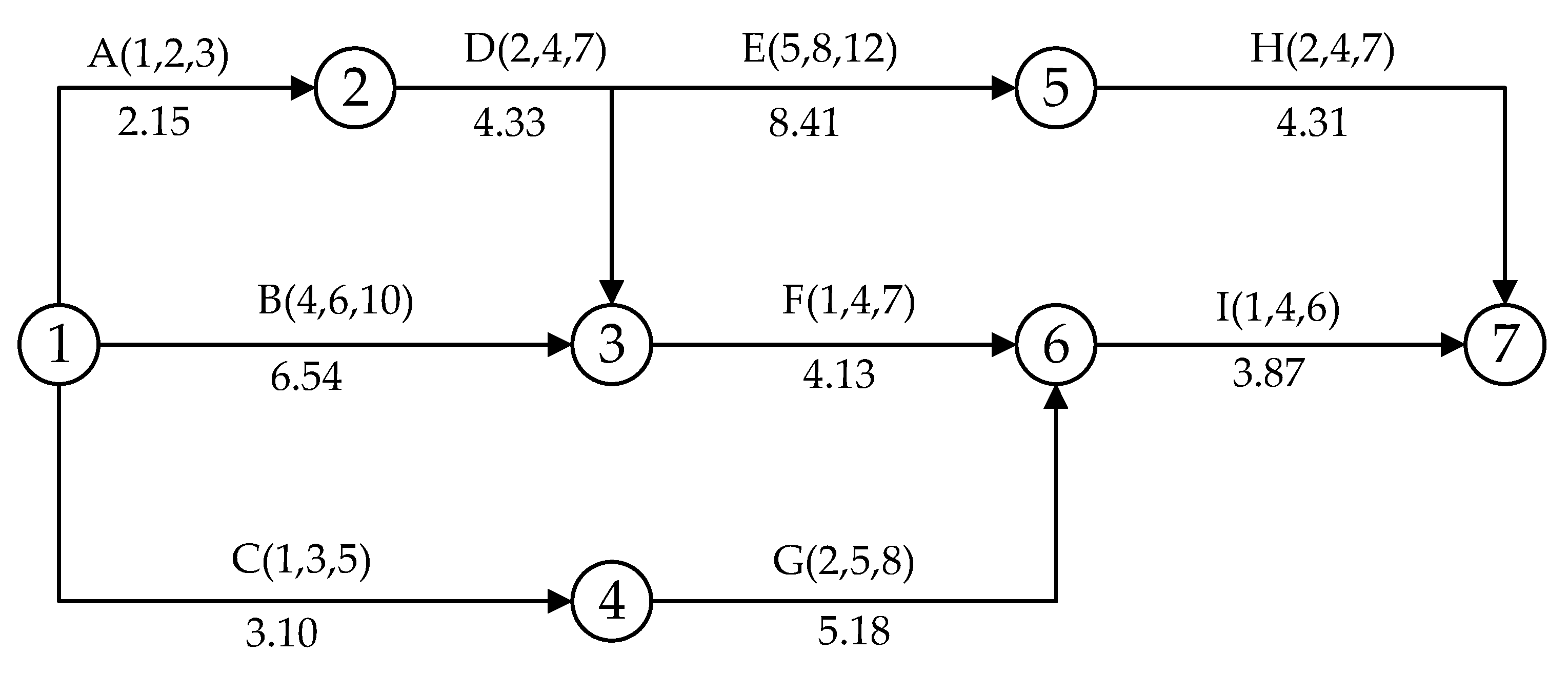
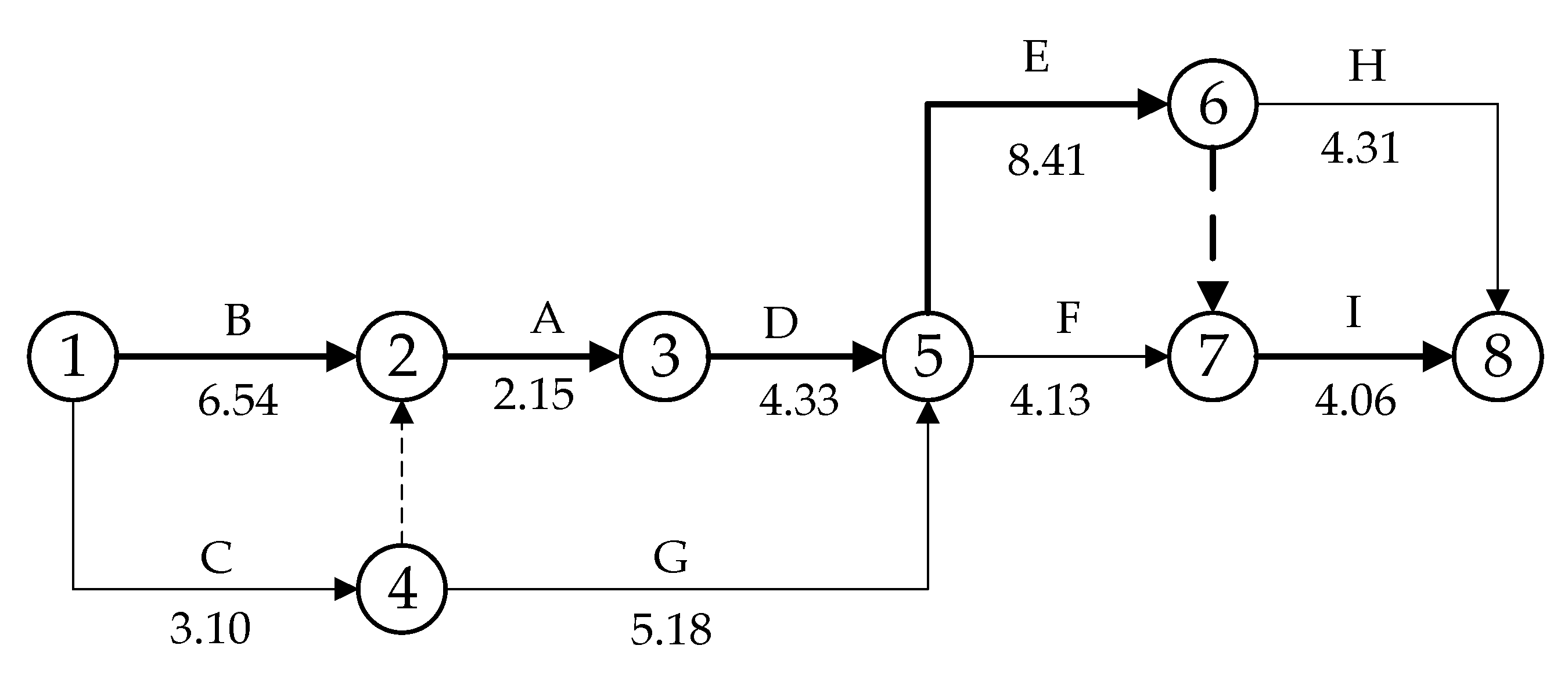
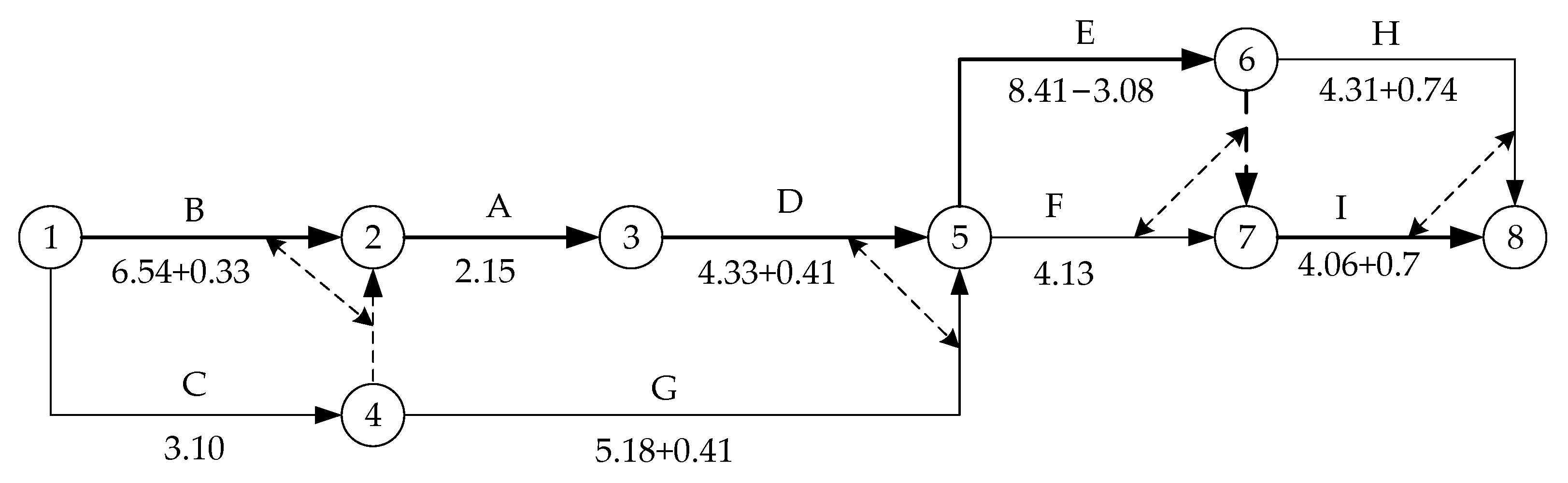
4.1. Example Introduction

There are nine A–I processes in the construction process of the foundation works of a project: the processes A–D are binding reinforcement 1–4; Processes E–G are formwork 1–3; Process H and process I are concrete pouring 1 and concrete pouring 2, respectively. The example process is the construction of slurry wall concrete cast-in-place pile of a project. The construction process has A–I nine processes: process A is preparing slurry; process B is to set the mud pool; process C is the preparation of site, machinery and materials; process D is burying the casing; process E is rotary drilling; process F is positive and negative circulation drilling; process G is steel cage prefabrication; process H is pouring concrete; process I is steel cage hoisting. The project site is about 45 km away from the central city. The indirect rate $\delta$ is RMB 20,000/d. The influence value E_i of each process on the environment shall not be greater than 1.20, and the safety level S_i shall not be lower than 0.95. The parameters of each process are shown in

Table 2. Parameters of each process process.

Process	Tia	Tim	Tib	Cia	Cimin	Ci	Qia	Qib	Qi	Pio	Piomax	Piomin
B	5.48	6.25	8.28	140.73	117.28	117.53	0.95	0.98	0.97	0.04	0.95	0.15
A	1.72	2.01	2.63	37.01	30.85	30.91	0.92	0.96	0.95	0.06	0.90	0.12
D	3.47	4.11	5.75	88.11	73.42	73.60	0.92	0.95	0.94	0.06	0.89	0.10
E	7.17	8.11	10.37	186.33	155.28	155.65	0.92	0.97	0.95	0.05	0.90	0.10
I	3.18	3.88	5.33	82.27	68.56	68.72	0.94	0.98	0.97	0.06	0.95	0.12
C	2.46	3.02	4.24	61.34	51.11	51.24	0.92	0.97	0.95	0.05	0.85	0.10
G	4.12	4.98	6.87	109.09	90.91	91.13	0.93	0.96	0.95	0.06	0.95	0.12
F	3.17	4.00	5.86	84.92	70.76	70.93	0.92	0.95	0.94	0.03	0.92	0.08
H	3.44	4.12	5.77	88.26	73.55	73.72	0.93	0.98	0.96	0.05	0.85	0.05

. The project requires three kinds of resources, and each process requires at least one resource. The resource demand of each process, the limit of each resource, and the resource constrained parameters are shown in

Table 3. Resource demand and resource influence coefficient of each process.

Process	Resource			λi	Ri
	1	2	3
A	4	1	1	0.26	0.15
B	6	0	1	0.08	0.13
C	2	0	0	0.17	0.23
D	2	1	1	0.33	0.51
E	5	1	1	0.16	0.19
F	3	0	1	0.12	0.01
G	4	0	1	0.20	0.10
H	4	0	1	0.16	0.07
I	3	1	0	0.17	0.08
Rk	8	1	2
wk	0.46	1.00	0.50

. Using Crystal Ball software for Monte Carlo simulation of each process, 5000 simulation results were extracted, and taking process B as an example, the frequency distribution of process B simulation results is shown in Figure 3. The green section represents the Beta PERT distribution probability density function with a minimum value equal to 4, a most likely value equal to 6, and a maximum value equal to 10 as the characteristic values. The blue section represents the results of 5000 simulations.

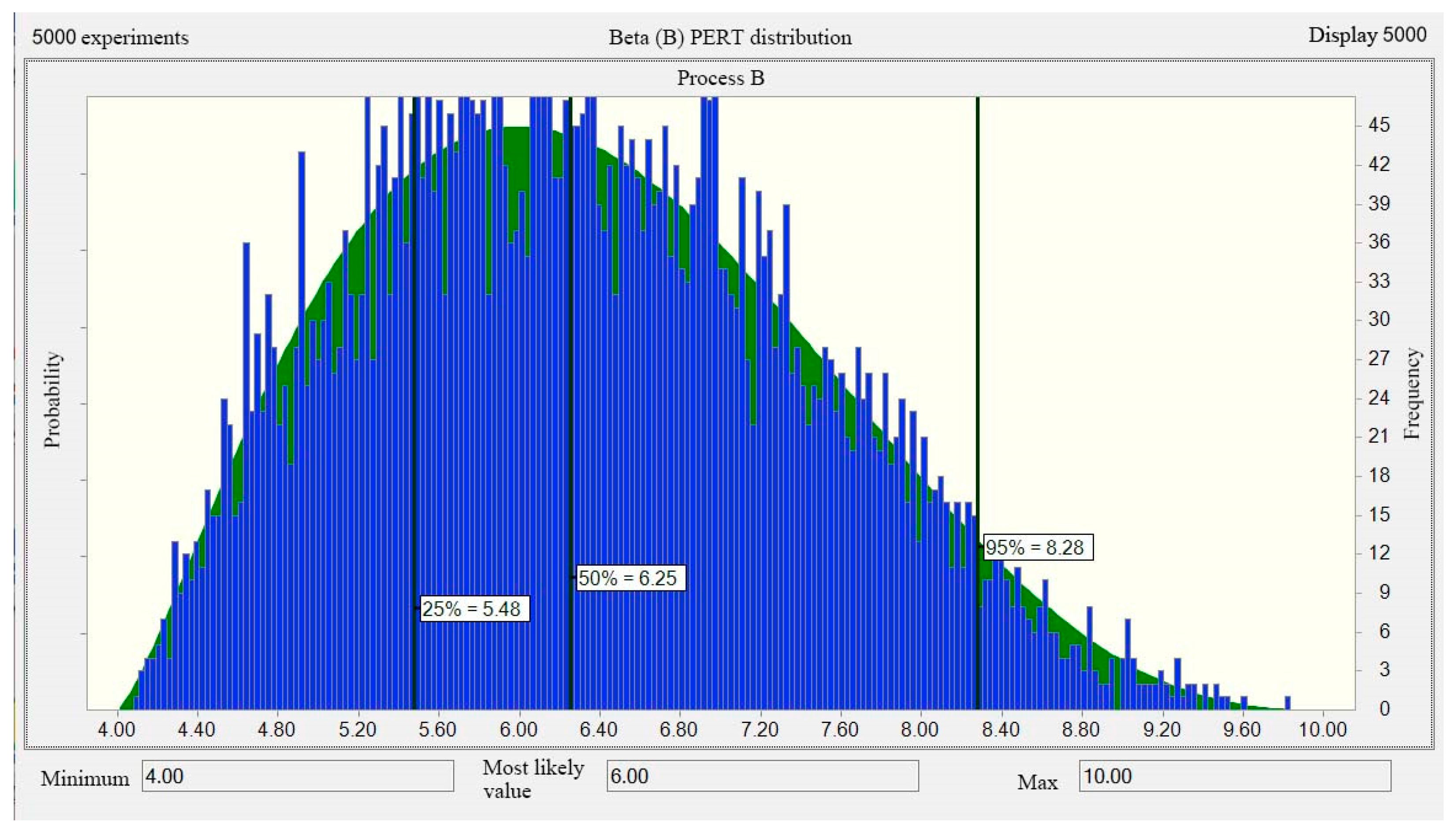
4.2. Process Safety Time under Multi-Objective Constraints

Taking process B as an example, process B is expected to last $T_B^C$ for 6.17 d under the constraint of target cost (C_B = RMB 1,175,300), $T_B^Q$ for 7.34 d under the constraint of target quality level (Q_B = 0.97), $T_B^S$ for 6.15 d under the constraint of target safety level (≥0.95), and $T_B^E$ for 6.50 d under the constraint of target environmental level (≤1.20), yielding Z_B = 6.54 d and ST_B = 1.74 d. The calculation of process safety time under multi-objective constraints is shown in

Table 4. Calculation of process safety time under multi-objective constraints.

Process	${\mathit{T}}_{\mathit{i}}^{\mathit{C}}$	${\mathit{T}}_{\mathit{i}}^{\mathit{Q}}$	${\mathit{T}}_{\mathit{i}}^{\mathit{S}}$	${\mathit{T}}_{\mathit{i}}^{\mathit{E}}$	Zi	STi
B	6.17	7.34	6.15	6.50	6.54	1.74
A	1.98	2.40	2.20	2.04	2.15	0.48
D	4.04	4.98	4.20	4.11	4.33	1.42
E	8.01	9.07	8.07	8.50	8.41	1.96
I	3.80	4.78	3.90	3.77	4.06	1.27
C	2.96	3.52	3.00	2.92	3.10	1.14
G	4.89	5.94	5.00	4.88	5.18	1.69
F	3.91	4.95	3.91	3.76	4.13	1.73
H	4.05	4.82	4.30	4.08	4.31	1.46

. The network schedule based on multi-objective constraints is shown in Figure 4.

4.3. Calculation of Resource Influence Coefficient

The resource demand and resource constrained parameters for each process are shown in Table 3. Taking process A as an example, from $r_A^1$ = 4, $r_A^2$ = 1, $r_A^3$ = 1, R¹ = 8, R² = 1, R³ = 2, we get $u_A^1$ = 4/8 = 0.5, $u_A^2$ = 1/1 = 1, $u_A^3$ = 1/2 = 0.5. From R¹ = 8, there are nine processes using resource 1, we get ${\overline{r}}^1$ = 3.67, w¹ = 3.67/8 = 0.46. From T_A = 2.15 d, T = 25.49 d, we get λ_A = 2.15/25.49 = 0.26, R_A = 0.15. The adjusted network schedule considering multi-resource constraints is shown in Figure 5 [27].

4.4. Calculation of Process Relay Potential

Taking process D and process G as examples, process D is staffed with one assistant engineer and three technicians; process G is staffed with one senior engineer and three technicians. The efficiency coefficients of the cooperation of personnel, material, and machine are β_D =0.9 and β_G = 0.85. The resource reserve coefficient is γ = 0.98. The difficulty of the processes are D_D = 0.8 and D_G = 0.9. The equipment allocation rate is M_D = M_G = 0.99. The equipment utilization rate is N_D = N_G = 0.95. The process durations are T_D = 4.33 d, T_G = 5.18 d. According to Equations (19–22), the average speed of the relay network of this project is $\overline{v}$ = 2.02, v_D = 1.12, v_G = 1.99. From “$\overline{v}$ > v_G > v_D, T_G > T_D, T_G + ($\overline{v}$ − v_G)T_G/v_G < T_D + (v − v_D)T_D/v_D” yields P_D = −0.41, P_G = −0.41. The network schedule considering the process relay potential is shown in Figure 6.

4.5. Calculation of Process Adjacency Information Entropy

Taking process A as an example, k_A = 3, k_B = 1, k_C = 2, k_D = 3 can be obtained from Equation (27); A_A = 6, A_B = 3, A_C = 6, A_D = 10 can be obtained from Equation (26); H_A = 1.02 can be obtained from Equations (24) and (25); ${{\displaystyle H}}_A^{*}$ = 0.55 can be obtained from Equation (28).

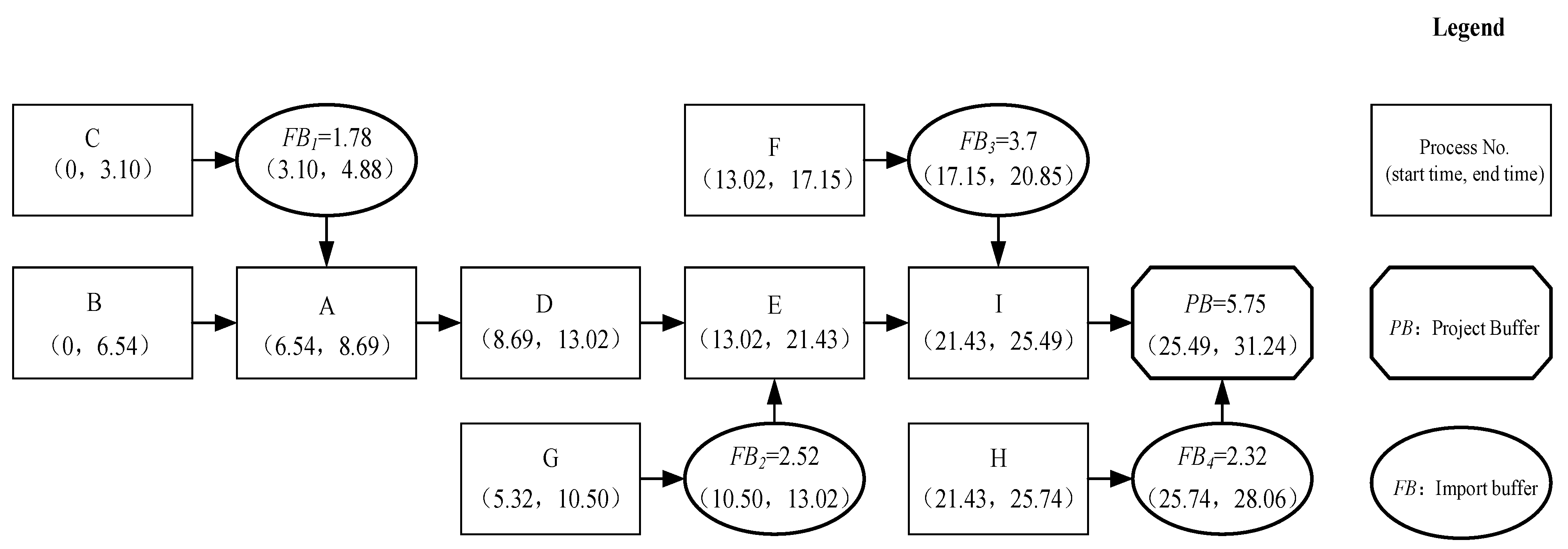
4.6. Calculation of Buffer Size

The initial project buffer of the critical chain and the initial import buffer of the non-critical chain are calculated from Equation (29), and the calculation results are shown in column 10 of

Table 5. Buffer Calculation Process.

Process Type (1)	Process (2)	Three-Time Estimate Distribution (3)	T95% (4)	Zi (5)	STi (6)	Ri (7)	${\mathit{H}}_{\mathit{i}}^{*}$ (8)	Li (9)	Buffer (10)	FFi (11)	FB (12)	KB (13)	PB (14)
Critical path process	B	(4, 6, 10)	8.28	6.54	1.74	0.15	0.066	−0.33	4.16	-	-	-	5.75
	A	(1, 2, 3)	2.63	2.15	0.48	0.13	0.550	-		-	-	-
	D	(2, 4, 7)	5.75	4.33	1.42	0.23	0.991	−0.41		-	-	-
	E	(5, 8, 12)	10.37	8.41	1.96	0.51	0.951	3.08		-	-	-
	I	(1, 4, 6)	5.33	4.06	1.27	0.19	0.518	−0.70		-	-	-
Non-critical path process	C	(1, 3, 5)	4.24	3.10	1.14	0.01	0.541	0.00	1.78	2.22	1.78	0
	G	(2, 5, 8)	6.87	5.18	1.69	0.10	0.991	−0.41	4.11	2.52	2.52	1.59
	F	(1, 4, 7)	5.86	4.13	1.73	0.07	1.003	0.00	3.70	4.28	3.70	0
	H	(2, 4, 7)	5.77	4.31	1.46	0.08	0.002	−0.74	2.32	-	2.32	0

. In this calculation example, only the initial import buffer of process G on the non-critical chain is greater than the free time difference. KB_G = 1.61 d and PB = 6.14 d can be obtained from Equations (32)–(34).

The planned project duration is 31.24 d, and the schedule of critical chain is shown in Figure 7.

4.7. Comparison and Analysis

The traditional cut-and-paste method, root variance method, Hu Chen’s method, and Chu Chunchao’s critical chain buffer calculation method are applied to the calculation and comparison in this article. The results calculated by this buffer calculation method and other buffer calculation methods are compared from the perspective of a project’s planned duration, import buffer, and project buffer size. The project schedule duration and critical chain buffer size under multiple buffer size calculation models are shown in

Table 6. Project schedule duration and critical chain buffer size under multiple buffer size calculation models.

Name of Methods	Factors Considered in the Method	Import Buffer (Day)				Project Buffer (Day)	Planned Project Duration (Day)
		FB1 (Process C)	FB2 (Process G)	FB3 (Process F)	FB4 (Process H)
Method used in this article	Multi-objective, multi-resource constraints, relay potential and adjacency information entropy	1.78	2.52	3.7	2.32	5.75	31.24
Hu Chen’s method	Project duration risks and multiple resource constraints	1.54	1.15	2.87	2.65	6.44	36.36
Chu Chunchao’s method	Resource utilization, project complexity, risk preference of decision-makers	2.06	4.11	4.52	4.11	11.60	35.60
Cut-and-paste	Safety time of activity	1.00	1.5	1.5	1.50	7.00	31.00
Root variance method	Variance of activity	2.00	3.00	3.00	2.00	6.78	30.78

. From Table 6, it can be concluded that: (1) The project schedule duration calculated by this model is larger than that calculated by the traditional cut-and-paste method and root variance method, but significantly smaller than that calculated by Hu Chen and Chu Chunchao’s methods; (2) The import buffer value calculated by this model is between the range of import buffer values calculated by Hu Chen and Chu Chunchao’s methods, and the size is moderate; (3) The project buffer value calculated by this model is close to the buffer values calculated by Hu Chen and traditional cut-and-paste method and root variance method, but much smaller than the buffer value calculated by Chu Chunchao’s method, which is consistent with the actual situation; (4) Limited by the small influence of the size and complexity of the example, if the project size and network complexity increase, the model can better reflect the rationality of the critical chain buffer size calculation model based on multi-objective constraints, multi-resource constraints, relay potential, and adjacency information entropy.

5. Conclusions

This study estimates the safety time of process based on the constraints of cost, quality, safety, and environment, which objectively reflects the risk of process duration. Considering the influence of process demand intensity, resource constraints, and process duration on the buffer size, it is more consistent with the influence of resource constraints on project construction schedule. Considering the influence of the relay potential of mutual cooperation and cross construction between processes on buffer size, the accuracy of buffer size setting is improved. Using the adjacency information entropy of processes to calculate the adjacency correlation complexity of different processes, a critical chain buffer size calculation model based on adjacency information entropy is proposed.

According to the comparative analysis of the calculation examples, the buffer calculation model of critical chain based on adjacency information entropy proposed in this study can reasonably control the size of the buffer and effectively shorten the project duration, and realize the resource scheduling and optimal allocation among the processes in the project. To a certain extent, it can guide construction enterprises to adopt scientific and reasonable methods to adjust the project schedule, thus improving the overall efficiency of construction enterprises. Therefore, the research on buffer calculation model of critical chain based on adjacency information entropy has certain practical value and guiding significance for the management level and development of construction enterprises.

There are two innovations of this study: ① On the basis of existing research, the relationship model of cost, quality, safety, environment, and process duration is improved, which improves the rationality and accuracy of process duration and safety time estimation and also improves the accuracy of buffer size setting. ② The adjacency information entropy is used to measure the correlation complexity of the process and its adjacent processes, which makes up for the deficiency of the existing research that only considers the correlation complexity of the process and its immediately preceding and following processes, and does not consider the influence of indirect adjacent processes.

The limitations of this study are: ① The research is based on certain reasonable assumptions. In the actual critical chain project management, there is a risk of dynamic changes in construction. At this time, the problem of buffer determination will be more complex. ② In the relationship model of cost, quality, safety, environment, and process duration, some other influencing factors are not considered. For example, in the relationship model between environment and process duration, the number of residents in the adjacent downtown area is not considered.

In future research, buffer monitoring and dynamic management are considered to be applied to the research of critical chain buffers. In addition, the relationship model of cost, quality, safety, environment, and process duration needs further research.

References

1. Bao, X.; Zhao, Y. Application of the Critical Chain Technique to the Project Scheduling Management. J. Lanzhou Jiaotong Univ. 2009, 28, 34–36. [Google Scholar]
2. Chen, W.; Zhang, S.; Wang, H. Project Cost, Progress and Quality Integrated Evaluation Based on Vector Angle Cosine. J. Civ. Eng. Manag. 2016, 33, 18–21+42. [Google Scholar] [CrossRef]
3. Goldratt, E.M. Critical Chain; The North River Press: Great Barrington, MA, USA, 1997. [Google Scholar]
4. Zhang, J.; Ran, W.; Jia, S.; Yang, S. Review and Prospect of Buffer Sizing of a Critical Chain Project. Manag. Rev. 2017, 29, 195–203. [Google Scholar] [CrossRef]
5. Herroelen, W.; Leus, R. On the merits and pitfalls of critical chain scheduling. J. Oper. Manag. 2001, 19, 559–577. [Google Scholar] [CrossRef]
6. Herroelen, W.; Leus, R.; Demeulemeester, E. Critical Chain Project Scheduling: Do Not Oversimplify. Proj. Manag. J. 2002, 33, 48–60. [Google Scholar] [CrossRef]
7. Newbold, R.C. Project Management in the Fast Lane: Applying the Theory of Constraints; CRC Press: Cleveland, OH, USA, 1998. [Google Scholar]
8. Tukel, O.I.; Rom, W.O.; Eksioglu, S.D. An investigation of buffer sizing techniques in critical chain scheduling. Eur. J. Oper. Res. 2006, 172, 401–416. [Google Scholar] [CrossRef]
9. Chu, C. Buffer sizing and critical chain project management. Comput. Integr. Manuf. Syst. 2008, 14, 1029–1035. [Google Scholar] [CrossRef]
10. Yang, L.; Li, S.; Huang, X.; Peng, T. A Buffer Sizing Approach in Critical Chain Scheduling with Attributes Dependent. Ind. Eng. Manag. 2009, 14, 11–14. [Google Scholar] [CrossRef]
11. Liu, S.; Luo, D.; Liu, J.; Chen, D. Research on The Critical Chain Buffer Setting Model of EPC Project. Oper. Res. Manag. Sci. 2015, 24, 270–280. [Google Scholar]
12. Hu, C.; Xu, Z.; Yu, J. Calculation Method of Buffer Size on Critical Chain with Duration Distribution and Multi—Resource Constraints. J. Syst. Manag. 2015, 24, 237–242. [Google Scholar]
13. Paprocka, I.; Czuwaj, W. Location Selection and Size Estimation of Resource Buffers in the Critical Chain Project Management Method. Appl. Mech. Mater. 2015, 809, 1390–1395. [Google Scholar] [CrossRef]
14. Ghoddousi, P.; Ansari, R.; Makui, A. A risk-oriented buffer allocation model based on critical chain project management. KSCE J. Civ. Eng. 2017, 21, 1536–1548. [Google Scholar] [CrossRef]
15. Nie, X.; Zheng, Y.; Gu, X.; Su, B.; Wang, B. Calculation of Buffer Size on Critical Chain Based on Duration Distribution, Multiresource Constraints, and Relay Potential. Sci. Program. 2022, 2022, 6591223. [Google Scholar] [CrossRef]
16. Zhang, J.; Jia, S.; Diaz, E. A new buffer sizing approach based on the uncertainty of project activities. Concurr. Eng. 2014, 23, 3–12. [Google Scholar] [CrossRef]
17. Zohrehvandi, S.; Khalilzadeh, M. APRT-FMEA buffer sizing method in scheduling of a wind farm construction project. Eng. Constr. Archit. Manag. 2019, 26, 1129–1150. [Google Scholar] [CrossRef]
18. Zohrehvandi, S.; Khalilzadeh, M.; Amiri, M.; Shadrokh, S. A heuristic buffer sizing algorithm for implementing a renewable energy project. Autom. Constr. 2020, 117, 103267. [Google Scholar] [CrossRef]
19. Marek-Kołodziej, K.; Łapuńka, I. A Fuzzy Method Determination of Time Buffer Size in Critical Chain Project Management. SSRN Electron. J. 2022. [Google Scholar] [CrossRef]
20. Lin, J.; Zhou, G. Study on Critical Chain Buffer Sizing Based on Uncertainty. Sci. Technol. Manag. Res. 2011, 31, 227–230. [Google Scholar]
21. Liu, D.Y.; Chen, J.G.; Peng, W. A New Buffer Setting Method Based on Activity Attributes in Construction Engineering. In Applied Mechanics and Materials; Trans Tech Publications Ltd.: Stafa, Switzerland, 2012; Volume 1801. [Google Scholar]
22. Zhang, J.; Song, X.; Yang, Y. Buffer Sizing of a Critical Chain Project Based on the Entropy Method. Manag. Rev. 2017, 29, 211–219. [Google Scholar] [CrossRef]
23. Zhang, J.; Zhou, S. Buffer Sizing of Critical Chain Projects Based on Uncertainty. J. Ind. Technol. Econ. 2021, 40, 154–160. [Google Scholar]
24. Liu, X.; Tian, G.; Fathollahi-Fard, A.M.; Mojtahedi, M. Evaluation of ships green degree using a novel hybrid approach combining group fuzzy entropy and cloud technique for the order of preference by similarity to the ideal solution theory. Clean Technol. Environ. Policy 2020, 22, 493–512. [Google Scholar] [CrossRef]
25. Wang, W.; Tian, G.; Zhang, T.; Jabarullah, N.H.; Li, F.; Fathollahi-Fard, A.M.; Wang, D.; Li, Z. Scheme selection of design for disassembly (DFD) based on sustainability: A novel hybrid of interval 2-tuple linguistic intuitionistic fuzzy numbers and regret theory. J. Clean. Prod. 2021, 281, 124724. [Google Scholar] [CrossRef]
26. Long, L.D.; Ohsato, A. Fuzzy critical chain method for project scheduling under resource constraints and uncertainty. Int. J. Proj. Manag. 2008, 26, 688–698. [Google Scholar] [CrossRef]
27. Liu, S.; Song, J.; Tang, J. Approach for setting time buffers in resources-constrained project scheduling. J. Syst. Eng. 2006, 21, 381–386. [Google Scholar]
28. Peng, W.; Lin, X.; Li, H. Critical chain based Proactive-Reactive scheduling for Resource-Constrained project scheduling under uncertainty. Expert Syst. Appl. 2023, 214, 119188. [Google Scholar] [CrossRef]
29. Du, X.; Zhao, W.; Lei, W. Comprehensive Optimization of Project Duration, Cost, Quality and Safety Based on Particle Swarm Optimization. Syst. Eng. 2019, 37, 139–150. [Google Scholar]
30. Yuan, J.; Mao, H.; Dai, K. Multi obiective Trade off of Green Construction Management under Nonlinear Relation. Sci. Technol. Prog. Policy 2017, 34, 33–37. [Google Scholar]
31. Hu, X.; Ma, P.; Gao, B.; Zhang, M. An Integrated Step-Up Inverter Without Transformer and Leakage Current for Grid-Connected Photovoltaic System. IEEE Trans. Power Electron. 2019, 34, 9814–9827. [Google Scholar] [CrossRef]
32. Ni, T.; Chang, H.; Song, T.; Xu, Q.; Huang, Z.; Liang, H.; Yan, A.; Wen, X. Non-Intrusive Online Distributed Pulse Shrinking-Based Interconnect Testing in 2.5D IC. IEEE Trans. Circuits Syst. II Express Briefs 2020, 67, 2657–2661. [Google Scholar] [CrossRef]
33. Ni, T.; Yao, Y.; Chang, H.; Lu, L.; Liang, H.; Yan, A.; Huang, Z.; Wen, X. LCHR-TSV: Novel Low Cost and Highly Repairable Honeycomb-Based TSV Redundancy Architecture for Clustered Faults. IEEE Trans. Comput. Aided Des. Integr. Circuits Syst. 2020, 39, 2938–2951. [Google Scholar] [CrossRef]
34. Han, Y.; Xu, H.; Jiang, J.; Yang, B. Time-cost-quality Joint Optimization Model of Construction Project Based on the Interval GERT Network. Syst. Eng. 2018, 36, 61–69. [Google Scholar]
35. Liu, X.; Chen, T.; Zhang, L. Application of PSO to multiple-objective project optimization. China Civ. Eng. J. 2006, 39, 122–126. [Google Scholar]
36. Zhang, L.; Luan, Y.; Zou, X. Time-cost-quality Trade-off Optimization Model of Construction Project. Syst. Eng. 2012, 30, 85–91. [Google Scholar]
37. Gheng, S.; Chang, K.; Tao, S. A Study on the Comprehensive multi-Objective Optimization of Construction Projects. J. Eng. Manag. 2022, 36, 107–112. [Google Scholar] [CrossRef]
38. Liu, J.; Liu, Y.; Shi, Y. Method of Time Cost Quality Tradeoff Optimization of Construction Project: A Study Based on Fuzzy Set Theory. J. Beijing Jiaotong Univ. Soc. Sci. Ed. 2017, 16, 30–38. [Google Scholar] [CrossRef]
39. Wang, B.; Zhou, H.; Li, Z. Relay chain network technology and its application. J. Hydroelectr. Eng. 2015, 34, 220–228+244. [Google Scholar]
40. Hu, G.; Xu, X.; Gao, H.; Guo, X. Node importance recognition algorithm based on adjacency information entropy in networks. Syst. Eng. Theory Pract. 2020, 40, 714–725. [Google Scholar]
41. Xu, X.; Han, W. The Setting Study for Feeding Buffer of Critical Chain Scheduling. Ind. Eng. Manag. 2007, 5, 51–55. [Google Scholar] [CrossRef]
Figure 1. Relationship between process cost and process duration.
Buildings 13 00942 g001
Figure 2. Relationship between process quality level and process duration.
Buildings 13 00942 g002
Figure 3. Frequency distribution of process B simulation results.
Buildings 13 00942 g003
Figure 4. Network schedule based on multi-objective constraints.
Buildings 13 00942 g004
Figure 5. Adjusted network schedule considering multi-resource constraints.
Buildings 13 00942 g005
Figure 6. Network schedule considering the process relay potential.
Buildings 13 00942 g006
Figure 7. Schedule of Critical Chain.
Buildings 13 00942 g007