Development of a Reliable Machine Learning Model to Predict Compressive Strength of FRP-Confined Concrete Cylinders

Abstract

The degradation of reinforced concrete (RC) structures has raised major concerns in the concrete industry. The demolition of existing structures has shown to be an unsustainable solution and leads to many financial concerns. Alternatively, the strengthening sector has put forward many sustainable solutions, such as the retrofitting and rehabilitation of existing structural elements with fiber-reinforced polymer (FRP) composites. Over the past four decades, FRP retrofits have attracted major attention from the scientific community, thanks to their numerous advantages such as having less weight, being non-corrodible, etc., that help enhance the axial, flexural, and shear capacities of RC members. This study focuses on predicting the compressive strength (CS) of FRP-confined concrete cylinders using analytical models and machine learning (ML) models. To achieve this, a total of 1151 specimens of cylinders have been amassed from comprehensive literature studies. The ML models utilized in the study are Gaussian process regression (GPR), support vector machine (SVM), artificial neural network (ANN), optimized SVM, and optimized GPR models. The input parameters that have been used for prediction include the geometrical characteristics of specimens, the mechanical properties of FRP composite, and the CS of concrete. The results of the five ML models are compared with nineteen analytical models. The results evaluated from the ML algorithms imply that the optimized GPR model has been found to be the best among all other models, demonstrating a higher correlation coefficient, root mean square error, mean absolute percentage error, mean absolute error, a-20 index, and Nash–Sutcliffe efficiency values of 0.9960, 3.88 MPa, 3.11%, 2.17 MPa, 0.9895, and 0.9921, respectively. The R-value of the optimized GPR model is 0.37%, 0.03%, 5.14%, and 2.31% higher than that of the ANN, GPR, SVM, and optimized SVM models, respectively, whereas the root mean square error value of the ANN, GPR, SVM, and optimized SVM models is, respectively, 81.04%, 12.5%, 471.77%, and 281.45% greater than that of the optimized GPR model.

1. Introduction

The rehabilitation and retrofitting of existing deteriorated and reinforced concrete (RC) structures are needs of the construction industry. RC structures need periodic maintenance to ensure their safety and serviceability [1,2]. The main reason behind the deterioration of RC structures is the corrosion mechanism. Corrosion affects the durability and safety of the structures. The structures built adjacent to coastal or marine environments are more prone to corrosion [3]. From various studies, it can be said that corrosion mostly occurs in 25-year-old existing structures [4]. Rebar corrosion occurs due to two reasons. Carbonation-induced corrosion is one of the key reasons; in this process, the carbon dioxide from the atmosphere reacts with the steel rebar which in turn initiates the process of corrosion. Due to the alkaline behavior of concrete material, a film of passivity is developed around the steel rebar. The penetration of carbon dioxide into concrete breaks the alkalinity of concrete, reduces pH, and diminishes the passive layer resulting in rebar corrosion. The second major reason for corrosion is chloride-induced corrosion. Chlorides from the marine environment ingress into concrete due to which the de-passivation of the steel rebar occurs [5]. The initiation of corrosion in the steel rebar induced through chlorides mainly depends on the coefficient of chloride diffusion of concrete [6]. Both corrosion mechanisms reduce the mass percentage area of the steel rebar which diminishes the ultimate strength of the structure [7,8].

Existing RC structures should meet loading requirements under critical conditions, resist corrosion, and sustain blast attacks. Therefore, from time to time, strengthening of structures should be done to improve the service life by following recommended codal provisions. The ACI Committee Report 546 [9] has given guidelines for the material selection for concrete repair. There are limited studies done on repairing concrete structures affected by corrosion [10]. Because of the upgradation and strengthening of the already-constructed structures, fiber-reinforced polymer (FRP) composites have attracted the attention of researchers across the world [11], and the lack of applications of conventional repairing material has led to the evolution of FRP [12]. Composites are considered promising materials for the retrofitting and repair of structural concrete. Composites are the combination of two or more material; one of them is the matrix phase, and the other is fiber such as Carbon, Glass, Aramid, Basalt, etc. [13]. The use of FRP in newly constructed structures as well as in prevailing RC structures has increased in past decades [14]. The FRP-confined concrete specimens depend on factors such as the specimens’ diameter $(D)$, the thickness of FRP ($t_f$), the tensile strength of FRP $(f_f)$, and the unconfined compressive strength (CS) of concrete ${(f}_{co}^{\prime })$.

Apart from the above-mentioned factors, other parameters, such as aggregate size and imperfections in the bond, also affect the properties of FRP composites. Recent research has proven that the CS of FRP-confined concrete is affected by utilizing coarse aggregate-free concretes as well. Jiang [15] explored different concrete types and observed their strength performance. The author used FRP-confined ultra-high-performance concrete (UHPC) and FRP-confined engineered cementitious composite (ECC) specimens. It was reported that the strength-enhancement coefficient of both types of concrete was almost identical due to FRP confinement. The author revealed that similar strength enhancement for FRP-confined UHPC, ECC, and mortar was due to the inexistence of coarse aggregate. Jiang et al. [16] examined the stress-strain behavior of FRP-confined concrete with aggregate size effects. The experiments were performed on concrete cylinders with different sizes of aggregates. It was concluded that aggregate size had no influence on the stress-strain behavior of unconfined cylinders but had a significant impact on the stress-strain curve of FRP-confined concrete. Jamatia and Deb [17] studied the size effect in FRP-wrapped specimens under axial loading. It was witnessed that large columns showed significant size effects, whereas cylindrical columns with smaller size ruptured due to plastic deformations in concrete. Khalil et al. [18] examined the response of circular silos used in industries to store the bulk of solid material with a greater storing capacity up to 1000 tons. The vulnerability of the failure modes of silos and cylindrical shells was assessed too. Several mitigation methods were employed to retrofit silos, and were classified into strengthening techniques, seismic isolation technique, and bulk material response improvement. Jamatia et al. [19] investigated the effects of imperfections in the bond on strength of FRP-wrapped cylindrical columns. It was noted that imperfections in the bond were responsible for deformations and reduced the capacity of FRP-confined concrete. Some insights on vulnerability and risk associated to cylindrical structures were also demonstrated in the study. In addition, Ruggieri et al. [20] conducted vulnerability studies on existing buildings in Italy. They used available photographs as input data to analyze vulnerability. The study involved collecting images from specific locations, labelling and storing them, training machine learning (ML) models to classify the images, ranking the images, and assigning a vulnerability index to each building. The researchers compared their results with manual computations using the same ML algorithms and found that the ML-based approach was effective.

FRP offers several advantages to the construction industry, for example, greater weight-to-strength ratio, non-corrodibility, ease of installation, lightweight, high durability, etc. The lightweight characteristic of FRP produces low construction costs with high efficiency. FRP acts as a promising composite technique for the strengthening and rehabilitation of RC structures, which enhances the working life of RC structures and is resistant to severe environmental actions [21]. Homam et al. [22] evaluated the effect of environmental conditions and the durability of FRP composite material. They found that FRP strongly resisted environmental actions. However, adverse changes in tensile strength were seen due to moisture interaction. The performance of FRP decrease when FRP is used at elevated temperatures, which has emerged as a major drawback of FRP. High-strength fiber embedded in epoxy resin undergoes the liquid-glass transition at higher temperatures. According to technical approvals and specification sheets, resin is safe to use up to +50 °C [23]. Other drawbacks include difficulty in applying the material to wet or cold surfaces, the high cost of epoxy resins, limited reversibility, insufficient vapor permeability, vulnerability to UV radiation, hazards for manual labor, diffusion tightness, and the need for skilled labors to properly apply FRP to a substrate. To overcome the aforementioned issues, the best alternative to FRP is fiber reinforced cementitious matrix (FRCM), which provides good bond behavior with the concrete substrate [24]. The epoxy-based organic resins are replaced by inorganic cement-based mortar, which offers several benefits in contrast to FRPs. The inorganic matrix has a number of advantages, such as good compatibility with the concrete substrate, heat and fire-resistance, applicability on wet and cold surfaces, economic strength higher than FRP, suitability for irregular or rough substrates, no requirement of skillful labors, and exhibition of sufficient vapor permeability and high reversibility.

ML models such as artificial neural network (ANN), Gaussian process regression (GPR), support vector machine (SVM), optimized GPR, and optimized SVM have been used in the current research work to predict the CS of FRP-confined concrete cylinders. This article is divided into six sections. In Section 1, the deterioration of the concrete structure, causes of degradation, FRP, and the ML models have been discussed. In Section 2, a literature review of the past studies and research significance of this work are reported. 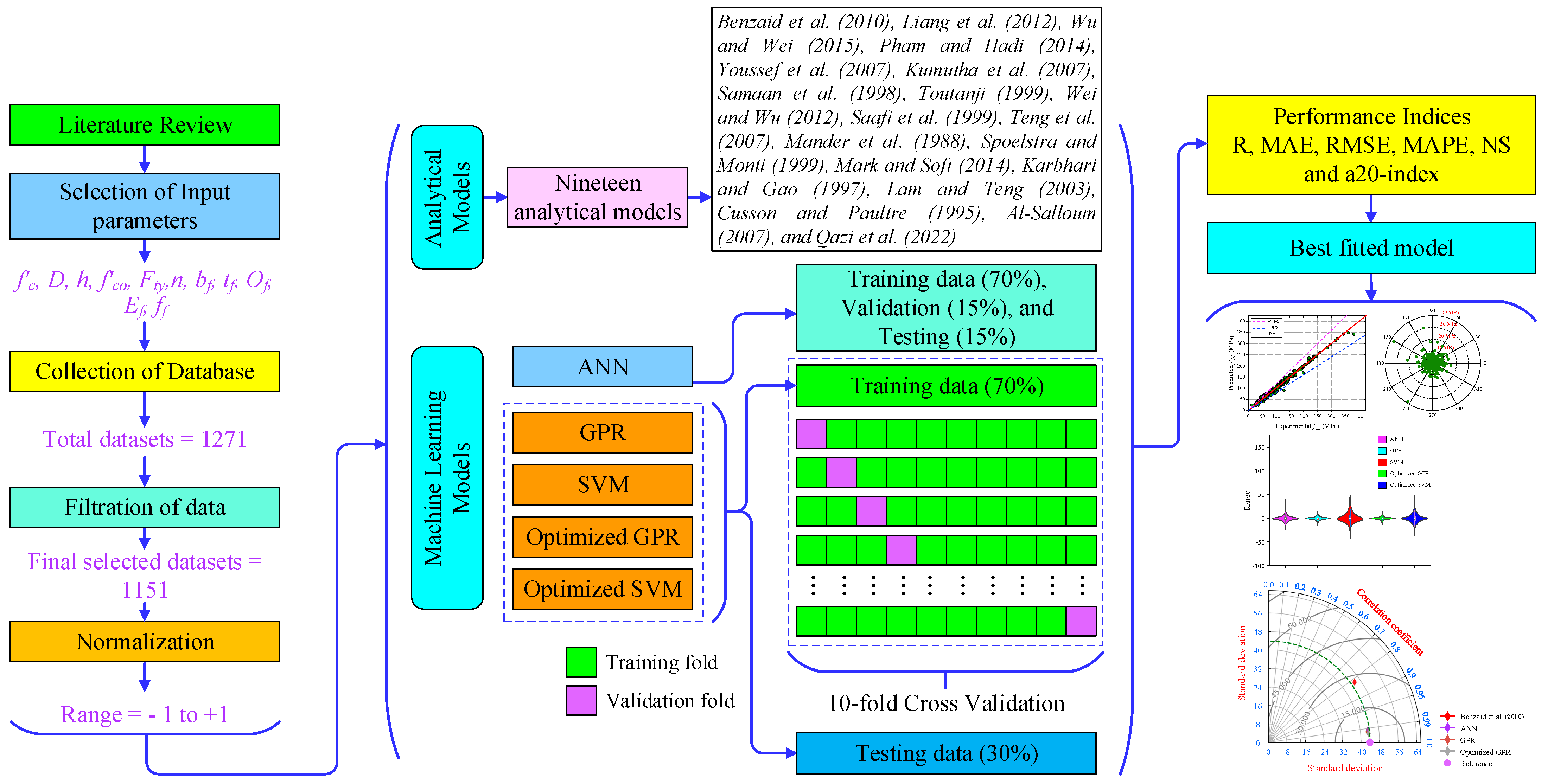Section 3 deals with the organization of this research work which includes database collection, processing of data, application of performance measures, analytical models of the FRP-confined concrete cylinders, and the ML models used in this study. Section 4 presents the results and discussion, including a comparison of the ML models with the existing models, and the formulation of the ML models. The conclusions and the future scope of the research are provided in Section 5. The objective of this study is to suggest a prediction model for the CS of concrete cylinders confined using FRP composite. However, previous research works have demonstrated comparable methods to estimate the CS of the FRP-confined concrete cylinders with a limited number of specimens. Therefore, this study utilizes a large database of 1151 specimens to develop the best ML model for prediction.

2. Literature Review

According to the survey of the literature, the available analytical models to predict the CS of the FRP-confined concrete cylinders are very limited. It has been observed that developed analytical relationships are dependent on a specific parameter; therefore, some specific limited databases are required to predict the CS of the FRP-confined concrete cylinders. Moreover, various assumptions were applied by researchers that reduce the efficiency of models. The development of robust and accurate models has become necessary to evaluate the FRP-wrapped CS of cylinders. Artificial intelligence (AI) has contributed to almost all the specializations of civil engineering such as concrete technology, structural health monitoring, green buildings, water management, hydropower plants, etc. [25,26,27]. One of the ways to develop efficient models is the application of AI in the computation of the confined CS. Some of the ML models developed by researchers are discussed below.

Cevik and Guzelbey [28] applied a neural network (NN) technique for the investigation of the confined CS of carbon-FRP (CFRP). A total of 101 databases were collected from seven literature studies. Input parameters taken from the studies include the cylinder’s diameter, unconfined CS, FRP’s tensile strength, and its thickness, whereas the confined CS of CFRP is considered to be the output parameter. The result proposed by the NN models was satisfactorily found to have an R-value equal to 0.98 when compared with the experimental results. Moreover, the CS predicted using the NN models was more accurate than the existing models. Gandomi et al. [29] investigated the ultimate confined CS of CFRP-wrapped cylindrical specimens using linear genetic programming (LGP). The authors utilized two sets of input databases, in which the first set consisted of $D,t,f_f,$ and $f_{co}^{\prime }$, and another set included $f_{co}^{\prime }$ and $P_u$. The results from the proposed formulation illustrated that the confined CS was found to be accurate and precise in comparison with the existing models. Naderpour et al. [30] carried out research on the confined CS of FRP-wrapped cylinders by using ANN. Several databases were collected from past literature to formulate a new proposed model. Authors employed various input variables in the study, such as $D,L,f_c^{\prime },t,f_{frp},$ and $E_{frp}$. The error percentage provided by the ANN models was less than 9%. The confined CS obtained from the developed formulation using ANN demonstrated good precision and accuracy when compared with the existing models.

Cevik et al. [31] examined the effect of stepwise regression (SR) and genetic programming (GP) to predict the CS of CFRP cylinders. The authors also used fifteen empirical models from the past literature and compared the results with predicted ML models. The proposed formulations were found to be satisfactory with respect to observed values. It was resulted that the suggested model was more precise and efficient in comparison with the results of the existing analytical models. Cevik [32] computed the confined CS of cylinders by using novel AI methods such as SR, GP, neuro-fuzzy, and NN. The experimental database of 180 specimens was taken from seventeen published studies. The authors took ten analytical models developed by researchers. It was pointed out that the results achieved by the suggested formulation of AI techniques were quite accurate and precise compared with the experimental and mathematical results. Elsanadedy et al. [33] predicted the CS and strain of cylinders with FRP confinement utilizing the regression and NN models. A single hidden layer of NN was prepared and training, testing, and validation of test results were accomplished by taking a total of 272 datasets of cylindrical specimens from the literature. It was found that the NN predictions were more accurate and precise than those of the mathematical relations developed by researchers. In addition, the obtained results were also better than the developed model in the study.

Jalal and Ramezanianpour [34] examined the enhancement of the CS of the FRP-confined concrete cylinders using ANN. A dataset of 128 specimens of concrete cylinders was chosen for the strength prediction. A total of six basic input parameters were considered to develop the ML models. Results from the proposed formulation were compared with five existing models, which revealed that the mean percentage error of the ANN model was about 10%. The results from the proposed ANN models were found to be more accurate and precise. Pham and Hadi [35] predicted the CS and strain of confined columns with square and rectangular cross-sections by implementing the ANN technique. The authors applied 104 datasets for the CS evaluation of FRP-wrapped rectangular columns and 69 datasets for the strain assessment of FRP confined square columns. The general correlation factor of the proposed model of rectangular and square columns was found to be 96% and 98%, respectively. Lim et al. [36] evaluated the confined CS of cylinders by applying GP. Based on the wide-ranging database accumulated to predict the accurate results, a large dataset of 832 cylinders was taken in the study. The models were examined by certain standard criteria, and it was found that the proposed model obtained by GP predicted the ultimate CS more accurately and precisely than those developed by experiments.

Mansouri et al. [37] predicted the CS and strain of cylinders using the radial basis neural network (RBNN), adaptive neuro-fuzzy inference system (ANFIS) with subtractive clustering (ANFIS-SC), ANFIS with fuzzy c-means clustering (ANFIS-FCM), and the M5 model tree (M5Tree). In computing the CS of the FRP-confined concrete cylinders, RBNN and ANFIS-FCM methods contributed same level of outcomes with respect to other applied methods, while for computing strain, ANFIS-SC was superior to other models. Mozumder et al. [38] utilized the support vector regression (SVR) technique to calculate the CS of the FRP-confined concrete cylinders. The authors employed the SVM technique to CFRP and GFRP in the study. The model proposed by the SVR approach was compared with the ANN models. The SVR models were found to be more accurate and precise in comparison with the ANN models. Kamgar et al. [39] investigated the ultimate FRP-wrapped cylindrical CS of cylinders by using the feed-forward back propagation neural network (FFBPNN) method. The authors chose 281 datasets based on published literature to test and train the network. A new formulation was proposed by utilizing the FFBPNN method and was equated with other existing models. The R-value obtained for the proposed formulation was found to be 0.9809 and the error percentage was very low (3.49%). The results indicated that the confined CS predicted by FFBPNN was more accurate and precise compared with the existing models.

Keshtegar et al. [40] established a novel hybrid model using the SVR and response surface model (RSM) to compute the CS of the FRP-confined concrete cylinders and axial strain. The authors collected the findings of 780 circular specimens from previously published studies. The collected data were categorized into the training phase (574 samples) and testing phase (191 samples). $D,H,t_f,f_{co}^{\prime },E_f,$ and ${\epsilon }_{h,rup}$ were the considered input parameters in the study for the strength prediction. The novel approach illustrates robust behavior compared with the other models with the lowest mean absolute error (MAE) and root mean square error (RMSE) values. Kumar et al. [41] investigated the CS prediction of the lightweight concrete (LWC) by using the GPR, optimized GPR, ensemble learning (EL), support vector machine regression (SVMR), optimized SVMR, and optimized EL algorithms. It had been noted that the optimized GPR was considered to be the best model with a high value of R (0.9803). The performance of the optimized SVMR and EL methods was also satisfactory with the R-values of 0.9777 and 0.9740, respectively. Kumar et al. [42] presented a study on sustainable concrete and evaluated its CS. Fly-ash-based geopolymer concrete was used and optimized SVM, GPR, and EL were accompanied by the linear regression (LR). The EL, SVM, and GPR methods were the applied prediction models. The maximum R-value of 0.9590 was attained by the optimized GPR model and outperformed all the models with an RMSE value of 1.7132 MPa.

Prediction of the CS of the FRP-confined concrete cylinders was undertaken by Jamali et al. [43]. A total of 1066 samples of cylinders were collected from the literature and ML models such as the multi-layer perceptron (MLP), SVR, and a combination of ANFIS with particle swarm algorithm (PSO) were used to evaluate the CS. In addition, the Kriging interpolation method was also utilized to calculate the CS of the FRP-confined concrete cylinders. The effective input variables taken in the study were $f_{co}^{\prime },H,D,E_f,F_f,$ and $t$ for the strength prediction. The authors have used eleven existing analytical models and compared the best analytical model with the ML models. The statistical measures taken in the study were mean error, standard deviation, mean square error (MSE), RMSE, absolute error (IAE), and total error. It was concluded that the Kriging method was found to be the best effective model with higher accuracy. The R-value obtained by the model was 0.985, whereas the SVR and MLP models acquired the second and third places, respectively, in terms of accuracy.

Table 1. Details of developed ML models to predict CS of FRP-confined concrete cylinders.

Reference	Input Parameters	ML Technique	${\mathit{f}}_{\mathit{c}\mathit{c}}^{\mathbf{\prime }}$ (MPa)	$\mathit{R}$ Value
Cevik and Guzelbey [28]	$D,nt,E_f,f_{co}^{\prime }$	ANN	—	0.98
Gandomi et al. [29]	$D,t,f_f,f_{co}^{\prime }$	LGP	33.8–137.9	0.9392
Naderpour et al. [30]	$D,L,f_c^{\prime },t,f_{frp},E_{frp}$	ANN	30.80–241	0.9439
Elsanadedy et al. [33]	$D,t_j,E_j,f_{ju},f_c^{\prime }$	ANN	—	0.95
Jalal and Ramezanianpour [34]	$d,h,t,E_{FRP},{\epsilon }_{rup},f_c^{\prime }$	ANN	31.40–303	0.9731
Mansouri et al. [37]	$D,t,f_{co}^{\prime },E_f$	RBNN, ANFIS-SC, ANFIS-FCM, M5 Tree	31.40–372.20	0.9503
Mozumder et al. [38]	$D,H,f_c^{\prime },t_{frp},f_{frp,u}$	SVR, ANN	40–303	0.9990
Keshtegar et al. [40]	$D,H,t_f,f_{co}^{\prime },E_f,{\epsilon }_{h,rup}$	RSM, SVR	24.1–372.2	0.9423
Jamali et al. [43]	$f_{co}^{\prime },H,D,E_f,F_f,t$	MLP, SVR, ANFIS-PSO, ANFIS, Kriging	17.8–381	0.985
Jalal et al. [44]	$d,h,t,E_{FRP},{\epsilon }_{rup},f_c^{\prime }$	MR, ANN, GP, ANFIS	31.40–303	0.9997
Ahmad et al. [45]	$D,H,nt,E_f,f_{co}^{\prime }$	ANN	18.5–302.2	0.912

displays the ability of the developed ML models to predict the CS of the FRP-confined concrete cylinders, as available in the literature. This table shows the input parameters selected by various researchers to develop the ML models. The table also lists the R-value and range of the CS of the FRP-confined concrete cylinders of the developed ML models.

CS is an important property of concrete. Predicting the CS of the FRP-confined concrete cylinders is a laborious work, and high-cost large test setups are required, which are time-consuming. For a large database, we cannot predict the CS using trial-and-error methods. In the literature, various analytical models are available and widely used to calculate the CS of concrete. Sometimes, these models are not able to predict accurate results due to the complexity of the design mix, code requirements, the type of FRP, orientation of FRP, other properties of FRP, etc. To overcome these issues, the application of AI is useful to predict the CS of the FRP-confined concrete cylinders. ML is one of the promising domains of AI in the field of computation. ML techniques not only produce accurate results but are also less time-consuming. In this research work, ML techniques such as ANN, GPR, SVM, optimized GPR, and optimized SVM are employed to accurately predict the CS of the FRP-confined concrete cylinders. This is the first study in which a large range of the FRP-confined CS datasets has been utilized to develop the ML model, and it increases the reliability of the proposed models.

3. Methodology

3.1. Details of Collected Database

From an extensive study of published literature on the FRP-confined concrete cylinders, an experimental database of 1151 specimens was collected [46,47,48,49,50,51,52,53,54,55,56,57,58,59,60,61,62,63,64,65,66,67,68,69,70,71,72,73,74,75,76,77,78,79,80,81,82,83,84,85,86,87,88,89]. Input parameters considered in this study are the diameter of the cylindrical specimen $(D)$, the height of the cylindrical specimen $(h)$, concrete grade $(f_c^{\prime })$, FRP type $(F_{ty})$, orientation of FRP $(O_f)$, unconfined CS of the concrete cylinder ${(f}_{co}^{\prime })$, FRP width ($b_f)$ and thickness ($t_f)$, modulus of elasticity of FRP ($E_f)$, FRP tensile strength $(f_f)$, and number of FRP layers ($n)$. The FRP-confined CS is taken as the output $(f_{cc}^{\prime })$.

$f_c^{\prime }$ ranges between 8 to 204 MPa with 49.37 MPa as an average value. D and h of the cylinders range from 50 mm to 310 mm and 100 mm to 1000 mm with a mean value of 142.9 mm and 294.15 mm, respectively. $f_{co}^{\prime }$ ranges from 6.2 MPa to 200 MPa with 49.32 MPa as a mean value. $F_{ty}$ used in the study are carbon, glass, aramid, and basalt with their $E_f$ ranges from 21.3 GPa to 251 GPa and $f_f$ ranges from 69 MPa to 4580 MPa. Moreover, CFRP is wrapped on 822 cylindrical specimens while glass-FRP (GFRP), aramid-FRP (AFRP), and basalt-FRP (BFRP) are applied on 267, 38, and 24 cylindrical specimens, respectively.

The number of FRP layers used in the collected database are in the range of 1 to 14 and having thicknesses of 0.0501 mm to 5 mm. The collected dataset contains both the unidirectional and bi-directional fibers. The number of specimens chosen for unidirectional orientation and bi-directional orientation of fibers are 1107 and 44, respectively. The statistical indicators of all variables are listed in

Table 2. Statistical indicators related to variables.

Parameters	Symbol	Unit	Min.	Mean	Max.	Std.	Type
CS of concrete	$f_c^{\prime }$	MPa	8	48.35	204	30.38	Input
Diameter	$D$	mm	50	144.40	310	38.60	Input
Height	$H$	mm	100	297.48	1000	106.77	Input
Unconfined CS	$f_{co}^{\prime }$	MPa	6.20	48.16	200	31.23	Input
Type of FRP	$F_{ty}$	-	1	1.36	4	0.65	Input
Number of FRP layers	$n$	-	0.30	2.43	14	1.86	Input
Width of FRP	$b_f$	mm	15	263.81	1000	141.89	Input
Thickness of FRP	$t_f$	mm	0.05	0.65	3.90	0.74	Input
Orientation of FRP	$O_f$	-	1	1.02	2	0.14	Input
Elastic modulus of FRP	$E_f$	GPa	21.30	171.10	251	84.97	Input
Tensile strength of FRP	$f_f$	MPa	69	3025.64	4580	1308.11	Input
Confined CS	$f_{cc}^{\prime }$	MPa	12.60	81.26	381	43.88	Output

, and the input variables selected for the research are displayed in Figure 1.

The heat plot elaborates on the R-value between the output and input variables. As depicted in Figure 2, the R-value is calculated for all the input parameters of the collected database. The value of R equal to 1 indicates a good correlation between the two values and vice versa. As demonstrated in Figure 2, the R-value between $f_{co}^{\prime }$ and $f_c^{\prime }$ is 0.96, which is the highest among all the parameters. Similarly, the R-value between $E_f$ and $f_f$ is 0.87, which is the second highest value. The worst R-value of 0.66 can be seen in between $F_{ty}$ and $E_f$. The R-value in between $f_{cc}^{\prime }$ and $f_c^{\prime }$, $f_{cc}^{\prime }$ and $f_{co}^{\prime }$, and $h$ and $D$ are found to be 0.71, 0.73, and 0.78, respectively. To evaluate the optimal ML, the adopted methodology can be seen clearly in Figure 3.

3.1.1. Data Filtration

Data filtration plays a significant part in defining the accuracy of the ML model. Most of the datasets contain unwanted and incomplete information, which causes obstructions in defining robust and accurate models. Therefore, all the data collected from the dataset are filtered and refined from a 1271 to 1151 dataset.

3.1.2. Processing of Data

Processing of data is a vital phase in the ML models in order to analyze the ML models without difficulty, since the dataset comes in a variety of units. This step of processing the dataset makes data easy to understand by the ML algorithms, which enhances the computational stability. Therefore, all the data collected from the literature have been normalized in the range of −1 to +1. The expression of normalization is given in Equation (1).

$$O_{normalized}=\left[2\times \frac{d-d_{min}}{d_{max}-d_{min}}\right]-1$$

(1)

where $O_{normalized}$ is the normalizing value, d is the original value, $d_{max}$ is the maximum value of data, and $d_{min}$ is the minimum value of data.

3.1.3. Splitting of Dataset

For the ANN algorithm, the dataset was grouped into training, testing, and validation sets. 70% of the data (805 samples) were utilized for the training phase, while 15% of data were used for the testing phase (173 samples) and the validation phase (173 samples). For the GPR, SVM, optimized GPR, and optimized SVM models, the set of the data was divided into two parts in the ratio of 7:3 to avoid any overfitting of data. For the training set, 70% of the data (805 cylinders) were considered, while 30% (345 cylinders) were utilized for the testing phase. 10-fold cross-validation was used to validate the SVM and GPR algorithms.

3.1.4. Performance Metrics

In this research, the overall outcome of the ML models is assessed by measures such as R, a20-index, Nash–Sutcliffe efficiency (NS), MAE, mean absolute percentage error (MAPE), and RMSE. When the R-value is nearer to unity, it illustrates better results while more than a 0.85 value suggests a positive output. It can be summarized from previously published studies that the lower values of MAE, MAPE, and RMSE, and higher values of R, a20-index, and NS represent positive outcomes of the models. The expressions of statistical indices [90,91] are given below:

$$R=\frac{{\sum }_{i=1}^N(E_i-\stackrel{-}{E})(P_i-\stackrel{-}{P})}{\sqrt{{\sum }_{i=1}^N{(E_i-\stackrel{-}{E})}^2{(P_i-\stackrel{-}{P})}^2}}$$

(2)

$$MAE=\frac{1}{N}\sum _{i=1}^N\left|E_i-P_i\right|$$

(3)

$$MAPE=\frac{1}{N}\sum _{i=1}^N\left|\frac{E_i-P_i}{E_i}\right|\times 100$$

(4)

$$RMSE=\sqrt{\frac{{\sum }_{i=1}^N{\left(E_i-P_i\right)}^2}{N}}$$

(5)

$$NS=1-\frac{\sum _{i=1}^N{(E_i-P_i)}^2}{\sum _{i=1}^N{(E_i-\stackrel{-}{P_i})}^2}$$

(6)

$$a20-index=\frac{m20}{N}$$

(7)

where N is the number of specimens in dataset, $E_i$ is the experimental value, $\stackrel{-}{E}$ is the mean of the measured values, $P_i$ is the predicted value, $\stackrel{-}{P}$ is the mean of predicted values, and $m20$ is the number of specimens with experimental and predicted values (ranges from 0.8 to 1.2).

Figure 3. Methodology of this study (Benzaid et al. [48], Liang et al. [58], Wu and Wei [92], Pham and Hadi [93], Youssef et al. [94], Kumutha et al. [95], Samaan et al. [96], Toutanji [97], Wei and Wu [98], Saafi et al. [99], Teng et al. [100], Mander et al. [101], Spoelstra and Monti [102], Mark and Sofi [103], Karbhari and Gao [104], Lam and Teng [105], Cusson and Paultre [106], Al-Salloum [107], and Qazi et al. [108]).

Figure 3. Methodology of this study (Benzaid et al. [48], Liang et al. [58], Wu and Wei [92], Pham and Hadi [93], Youssef et al. [94], Kumutha et al. [95], Samaan et al. [96], Toutanji [97], Wei and Wu [98], Saafi et al. [99], Teng et al. [100], Mander et al. [101], Spoelstra and Monti [102], Mark and Sofi [103], Karbhari and Gao [104], Lam and Teng [105], Cusson and Paultre [106], Al-Salloum [107], and Qazi et al. [108]).

3.2. Details of Analytical Models

Many researchers in the past have developed an analytical relationship to calculate the CS of the FRP-confined concrete cylinders. This work presents nineteen analytical models from the published studies [48,58,92,93,94,95,96,97,98,99,100,101,102,103,104,105,106,107,108]. The empirical relationships include inputs such as unconfined CS, FRP thickness, the diameter of cylindrical specimen, confinement pressure, the tensile strength of FRP, and the modulus of elasticity of FRP, and the effects of these inputs on the confined CS have been investigated.

Wu and Wei [92] proposed a steel or FRP-confined model to predict the CS of the FRP-confined concrete cylinders. The novel characteristics of this model were its continuity and simplicity in predicting the continuous stress-strain curves for hardening and softening phases. This model was the extension of the Popovics’s model developed in 1973. The suggested model demonstrated superiority and flexibility in performance when validated and related to the existing relationships. Pham and Hadi [93] collected 574 specimens of RC columns confined with various FRPs and generated an FRP-confined model for concrete having conventional and high strength. The results obtained from the prediction of the models fitted the experimental results from the collected dataset. Youssef et al. [94] established a relationship for FRP-confined columns. The authors used circular- and rectangular-shaped large-scale columns with high confinement ratios. Kumutha et al. [95] proposed the simplest analytical relationship to explore the behavior of GFRP reinforced rectangular columns. They found that the predicted model best fitted with measured values. Samaan et al. [96] suggested a constitutive relationship for the prediction of FRP-reinforced columns in unidirectional and lateral directions. The results indicated that the predicted model provided a strong connection with measured values. Wei and Wu [98] presented constitutive unified relations to compute the ultimate stress and strain of FRP-confined concrete columns having rectangular, circular, and square specimens. Teng et al. [100] established a stress-strain model for FRP-confined concrete columns. The results of this novel model were applicable to wrapped and un-wrapped concrete specimens. In addition, the results were not only valid for FRP-confined concrete but also for varying confined materials. Mander et al. [101] provided a stress-strain relation for concrete confined in axial and lateral directions. The lateral confinement was applied with steel ties (spiral or circular). The results were measured under axial and cyclic loading conditions. Spoelstra and Monti [102] considered a uniaxial analytical relationship for FRP-confined concrete with steel jacketing as transverse confinement. Karbhari and Gao [104] proposed a uniaxial model, and considered FRP wraps, fiber orientation, and types of fiber to improve the CS of the FRP-confined concrete cylinders and found that the predicted model showed a good bond with measured values. Lam and Teng [105] reported a simple stress-strain model for FRP-confined concrete subjected to static and seismic loadings. The detailed information and formulation of each model is summarized in

Table 3. Analytical models with description.

S. No.	Reference	Formulation	Description
1	Benzaid et al. [48]	$\frac{f_{cc}^{\prime }}{f_{co}^{\prime }}=[1+1.60(\frac{f_l}{f_{co}^{\prime }})$]	$f_l=2\frac{f_f{t}_f}{D}$
2	Liang et al. [58]	$f_{cc}^{\prime }=f_{co}^{\prime }[1+(2.61-0.01f_{co}^{\prime })$($\frac{f_l}{f_{co}^{\prime }})$]	$f_l=2\frac{f_f{t}_f}{D}$
3	Wu and Wei [92]	$f_{cc}^{\prime }=f_{co}^{\prime }[0.75+2.7{\left(\frac{f_l}{f_{co}^{\prime }}\right)}^{0.9}]$	$f_l=2\frac{f_f{t}_f}{D}$
4	Pham and Hadi [93]	$f_{cc}^{\prime }=0.7f_{co}^{\prime }+1.8f_l+5.7\frac{t}{D}+13$	−
5	Youssef et al. [94]	$\frac{f_{cc}^{\prime }}{f_{co}^{\prime }}=[1+2.25({\frac{f_l}{f_{co}^{\prime }})}^{\frac{5}{4}}]$	CEF = $\frac{f_{cc}^{\prime }}{f_{co}^{\prime }}$; CR = $\frac{f_l}{f_{co}^{\prime }}$
6	Kumutha et al. [95]	$f_{cc}^{\prime }=f_{co}^{\prime }+0.93f_l$	$f_l=2\frac{f_f{t}_f}{D}$
7	Samaan et al. [96]	$f_{cc}^{\prime }=f_{co}^{\prime }$ + 6.0$f_l^{0.7}$	$f_l=2\frac{f_f{t}_f}{D}$
8	Toutanji [97]	$\frac{f_{cc}^{\prime }}{f_{co}^{\prime }}$ = [1 + 3.5(${\frac{f_l}{f_{co}^{\prime }})}^{0.85}$]	$f_l=2\frac{f_f{t}_f}{D}$
9	Wei and Wu [98]	$\frac{f_{cc}^{\prime }}{f_{co}^{\prime }}$= [0.5 + 2.7(${\frac{f_l}{f_{co}^{\prime }})}^{0.73}$]	$f_l=2\frac{f_f{t}_f}{D}$
10	Saafi et al. [99]	$\frac{f_{cc}^{\prime }}{f_{co}^{\prime }}$= [1 + 2.2(${\frac{f_l}{f_{co}^{\prime }})}^{0.84}$]	$f_l=2\frac{f_f{t}_f}{D}$
11	Teng et al. [100]	$\frac{f_{cc}^{\prime }}{f_{co}^{\prime }}=[1+3.5(\frac{f_l}{f_{co}^{\prime }})]$	$f_l=2\frac{f_f{t}_f}{D}$
12	Mander et al. [101]	$f_{cc}^{\prime }=f_{co}^{\prime }(2.254\sqrt{1+7.94\frac{f_l}{f_{co}^{\prime }}}$ $-2\frac{f_l}{f_{co}^{\prime }}$ $-1.254)$	$f_l=2\frac{f_f{t}_f}{D}$
13	Spoelstra and Monti [102]	$f_{cc}^{\prime }=f_{co}^{\prime }(0.2+3\sqrt{\frac{f_l}{f_{co}^{\prime }}}$)	$f_l=2\frac{f_f{t}_f}{D}$
14	Mark and Sofi [103]	$\frac{f_{cc}^{\prime }}{f_{co}^{\prime }}$ $=1.1+$3.23($\frac{f_l}{f_{co}^{\prime }}$)	CEF = $\frac{f_{cc}^{\prime }}{f_{co}^{\prime }}$; CR = $\frac{f_l}{f_{co}^{\prime }}$
15	Karbhari and Gao [104]	$f_{cc}^{\prime }=f_{co}^{\prime }[1+2.1({\frac{f_l}{f_{co}^{\prime }})}^{0.87}]$	$f_l=2\frac{f_f{t}_f}{D}$
16	Lam and Teng [105]	$f_{cc}^{\prime }=f_{co}^{\prime }[1+3.3(\frac{f_l}{f_{co}^{\prime }})$]	$f_l=2\frac{f_f{t}_f}{D}$
17	Cusson and Paultre [106]	$f_{cc}^{\prime }=f_{co}^{\prime }+2.1f_{co}^{\prime }({\frac{f_l}{f_{co}^{\prime }})}^{0.7}$	$f_l=2\frac{f_f{t}_f}{D}$
18	Al-Salloum [107]	$\frac{f_{cc}^{\prime }}{f_{co}^{\prime }}=[1+2.312(\frac{f_l}{f_{co}^{\prime }})$]	$f_l=2\frac{f_f{t}_f}{D}$
19	Qazi et al. [108]	$f_{cc}^{\prime }=f_{co}^{\prime }$+ 3.2$f_l$	$f_l=2\frac{f_f{t}_f}{D}$

.

3.3. ML Models

This section describes the implementation of the ML methods to predict the CS of the FRP-confined concrete cylinders. ML is the branch of AI in which innovatory and difficult tasks are processed by building algorithms. The ML algorithms employ computational approaches in which information is directly obtained from datasets rather than relying on an analytical model.

The architecture of the ML models is displayed in Figure 4. The ML methods (ANN, GPR, SVM, optimized GPR, and optimized SVM) used in the proposed research are described below:

3.3.1. ANN

ANN is the prominent technique used in ML. ANN contains simple processing units called neurons that are based on the human brain. The first artificially created neuron was proposed by McCulloch and Pitts in 1943 [109]. ANN is a series of interconnected large numbers of neurons or nodes having different weights. Neurons in the network receive signals as multi-layered input, process it, and send output signals to the brain. Each neuron receives multiple inputs from the information that is locally available at the nodes and transmits its output to the other nodes. Artificial neuron has a specific function called as a function of activation, and the output signal is generated when weighted input data cross the threshold limit. When the input value is zero, there is no output received, but when the input crosses the threshold limit, the output is generated [110].

Feed-forward neural network (FFNN) is one of the types of ANN. FFNN comprises of inputs received from different nodes, hidden layers, and output of the problem [111]. One of the most common families of FFNN is MLP. In MLP, neurons are arranged unidirectionally and have a static function that gives a single set of output [112]. The hidden layer builds non-linearity between input and output variables which can be achieved by activation functions [113]. These functions are written as:

$$Tansig=\frac{2}{1+e^{-2x}}-1$$

(8)

$$Purelin=f\left(x\right)=x$$

(9)

3.3.2. GPR

Gaussian process is the combination of an infinite number of random variables representing mean and covariance functions [114]. GPR is widely used in the ML applications due to its flexibility and intrinsic uncertainty measures over predictions [90]. Gaussian process can be found below:

$$f\left(x\right)\sim GP\left(\mu \left(x\right),k\left(x,x^{\prime }\right)\right)$$

(10)

In the above equation, $\mu \left(x\right)$ and $k\left(x,x^{\prime }\right)$ represent the mean function and covariance function, respectively. The mean function is assumed to be zero because the Gaussian process is the function of a linear combination of random variables. $k\left(x,x^{\prime }\right)$ is defined as a positive semi-definite kernel function, which is the covariance between $f\left(x\right)$ and $f\left(x^{\prime }\right)$, as shown below:

$$k\left(x,x^{\prime }\right)=cov\left(f\left(x\right),f\left(x^{\prime }\right)\right)$$

(11)

$\mu \left(x\right)=0$ (assumed), and the kernel has variable $\theta$, i.e., $k\left(x,x^{\prime }\left|\theta \right.\right)$. For a finite range of inputs $X=\left(x_1,x_2,\dots ,x_N\right)$, the function values $f\left(x\right)={\left(f\left(x_1\right),f\left(x_2\right),\dots ,f\left(x_N\right)\right)}^T$ have joint multivariate Gaussian distribution:

$$f(X)~N\left(0,k_{X,X}(\theta )\right)$$

(12)

where elements of N-by-N covariance matrix are defined by the kernel:

$${\left[k_{X,X}\left(\theta \right)\right]}_{i,j}=k\left(\left.x_i,x_j\right|\theta \right)$$

(13)

All the above formulations of Gaussian process were taken from [115]. The covariance function is expressed as below:

$$k\left(x,x\prime \right)={\sigma }_f^{2}exp\left[\frac{-r}{2}\right]$$

(14)

where r is illustrated in the below equation:

$$r=\frac{{\left|x-x^{\prime }\right|}^2}{l^2}$$

(15)

${\sigma }_f$ and l indicate the model noise and length scale, respectively, which also are the hyper-parameters that affect the outcome of the Gaussian process. Various kernel functions applied in this investigation are Matern 3/2, Matern 5/2, Exponential, and Rational Quadratic. All the details of the kernel functions are given in Asante-Okyere et al. [114]. The optimized GPR model is displayed in Figure 5.

3.3.3. SVM

SVM is a promising ML technique developed by Vladimir Vapnik in 1995 [116,117]. The SVM is generally based on linear functions and called linear SVM (LSVM). Initially, it was designed on the basis of recognition patterns but through SVM, small sub-sets can be created from a large number of training data. These smaller subsets are known as support vectors (SVs). SVs are always smaller than the total samples taken in the study. SVs are used to compute the values with the least error of margin [118]. Therefore, the SVM technique is the simplest among other ML methods such as GPR, ANN, etc. The non-linear classification of SVM is developed by introducing a kernel function called as non-linear SVM (NSVM).

For the given dataset $\left\{\left(x_1,y_1\right),\left(x_2,y_2\right),\dots ,\left(x_i,y_i\right),\dots ,\left(x_N,y_N\right)\right\}$ where $x_iϵR^n$ are input values, $y_iϵR^n$ are corresponding output values, and $N$ is number of datasets, LSVM for the LR problem can be written as:

$$y=f\left(x\right)=w.\varphi \left(x\right)+b$$

(16)

where $w$ is the weight vector, $\varphi \left(x\right)$ elaborates mapping function, and b represents the bias parameter:

$$y_i=\sum _{i=1}^n\left({\alpha }_i-{\beta }_i\right)\times \left(x,x_i\right)+b$$

(17)

where ${\alpha }_i$ and ${\beta }_i$ indicate the Lagrange multipliers. In case of non-linearity, the kernel function is introduced.

$$y_i=\sum _{i=1}^n\left({\alpha }_i-{\beta }_i\right)\times k\left(x,x_i\right)+b$$

(18)

where $k\left(x,x_i\right)$ is the kernel function.

The optimized SVM model for the proposed work is depicted in Figure 6.

4. Results and Discussion

The implementation of the ML algorithms (ANN, GPR, SVM, optimized GPR, and optimized SVM) on 1151 cylindrical specimens is presented and discussed in this section. The performance of these algorithms is measured using six different metrics, i.e., R, MAE, a20-index, RMSE, NS, and MAPE. The outcomes of the suggested analytical models are displayed and described with the help of a scatter plot, a violin plot of error distribution, and a Taylor diagram.

4.1. Results of Analytical Models

The performance indices of all the analytical models are listed in

Table 4. Statistical indicators of analytical models.

S. No.	Reference	R	MAPE (%)	MAE (MPa)	RMSE (MPa)	a20-Index	NS
1	Benzaid et al. [48]	0.8177	25.75	19.05	27.02	0.5065	0.6205
2	Kumutha et al. [95]	0.8342	24.61	20.15	27.70	0.4352	0.6356
3	Pham and Hadi [93]	0.7651	26.77	18.98	29.70	0.5942	0.5441
4	Samaan et al. [96]	0.8345	31.52	21.11	29.17	0.5560	0.6007
5	Wei and Wu [98]	0.8041	29.04	20.33	31.40	0.5873	0.5040
6	Spoelstra and Monti [102]	0.8446	30.91	22.05	31.45	0.5551	0.5343
7	Karbhari and Gao [104]	0.8297	30.70	21.76	32.30	0.5543	0.5064
8	Liang et al. [58]	0.7114	31.07	21.20	37.15	0.6378	0.3264
9	Saafi et al. [99]	0.8334	32.66	23.17	34.16	0.5473	0.4710
10	Wu and Wei [92]	0.7674	32.41	22.26	38.77	0.6370	0.2935
11	Cusson and Paultre [106]	0.8542	34.38	25.01	33.80	0.4622	0.4970
12	Al-Saloum [107]	0.7794	32.67	22.65	38.42	0.5994	0.3200
13	Mander et al. [101]	0.8523	48.54	36.26	46.70	0.2980	0.2573
14	Youssef et al. [94]	0.6572	34.01	23.68	47.96	0.5769	−0.1205
15	Qazi et al. [108]	0.7334	49.76	35.50	59.51	0.4787	−0.1403
16	Lam and Teng [105]	0.7289	52.18	37.40	62.07	0.4466	−0.1836
17	Toutanji [97]	0.7922	63.07	46.24	65.34	0.2710	−0.0603
18	Mark and Sofi [103]	0.7462	55.80	40.40	63.54	0.3918	−0.1503
19	Teng et al. [100]	0.7200	57.23	41.37	67.25	0.4014	−0.2633

. The predicted model can be termed as accurate when the error values of MAE, MAPE, and RMSE are lowest, and the R, NS, and a20-index values are higher. According to Table 4, the model of Benzaid et al. [48] has a better performance based on the performance criteria. The highest rank achieved by the model of Benzaid et al. [48] with an R-value of 0.8177 and RMSE, MAE, MAPE, NS, and a20-index values of 27.02 MPa, 19.05 MPa, 25.75%, 0.6205, and 0.5065, respectively. The second-best optimal model is recognized as the model of Kumutha et al. [95] with an R-value (0.8342), RMSE (27.70 MPa), MAE (20.15 MPa), MAPE (24.61%), NS (0.6356), and a20-index (0.4352) values. Moreover, the maximum R-value (0.8542) is obtained by the model of Cusson and Paultre [106], while the worst R-value (0.6572) is attained by the model of Youssef et al. [94]. The model of Teng et al. [100] has the worst performance according to the performance metrics with R, RMSE, MAE, MAPE, a20-index, and NS values of 71.99%, 67.25 MPa, 41.37 MPa, 57.23%, 0.4014, and −0.2633, respectively. In Table 4, the sequence of the analytical models has been arranged according to the accuracy of the models.

The outcomes of the confined CS of each model are presented in Figure 7, which depicts a scatter diagram between the measured and predicted CS of the FRP-confined concrete cylinders. The results provided in Figure 7 illustrate that the data points in the best-predicted model are uniformly concentrated on the best fitted line and show superior accuracy. According to this figure, the data points in the model of Wu and Wei [92] are lying above the diagonal line, which indicates that the model overestimates the confined CS of the cylinder. However, a good proportion of the data points in the models of Pham and Hadi [93] and Youssef et al. [94] are evenly scattered on both sides of the straight line. It has been observed that almost all the data points in the model of Kumutha et al. [95] are lying beneath the diagonal line, demonstrating that the model underestimates the confined CS of the FRP-confined concrete cylinders, whereas, in the models of Samaan et al. [96] and Toutanji [97], a good proportion of the data points are scattered above the diagonal line, signifying that the models overestimate the CS of the FRP-confined concrete cylinders. It has also been witnessed that most of the data points in the model of Wei and Wu [98] are uniformly distributed along the best fitted line, indicating good accuracy of the model.

The scatter diagram shows that most of the data points in the models of Saafi et al. [99], Teng et al. [100], Mander et al. [101], Spoelstra and Monti [102], Mark and Sofi [103], Karbhari and Gao [104], Lam and Teng [105], Cusson and Paultre [106], Liang et al. [58], Al-Saloum [107], and Qazi et al. [108] are lying above the diagonal straight line which clarifies that these models overestimate the confined CS of concrete. However, a highly concentrated uniform distribution of the data points is observed in the model of Benzaid et al. [48] indicating that the model has the maximum predictive accuracy.

4.2. Results of ML Models

Five ML models (ANN, GPR, SVM, optimized GPR, and optimized SVM) have been established to predict the CS of the FRP-confined concrete cylinders. The model’s performance has been assessed using six performance indices as mentioned in Section 3.1.4.

In ANN, a single hidden layer has been used with neurons from 3 to 34. The best neuron has been selected with the trial-and-error method.

Table 5. Comparison of ML models based on statistical parameters.

Model		R	MAPE (%)	MAE (MPa)	RMSE (MPa)	a20-Index	NS
ANN	Training	0.9945	4.86	3.22	4.49	0.9826	0.9890
	Testing	0.9887	7.08	4.94	7.51	0.9480	0.9771
	Validation	0.9845	7.02	4.85	7.43	0.9306	0.9690
	All	0.9919	5.51	3.72	5.55	0.9696	0.9840
GPR	Training	0.9979	2.69	1.78	2.79	0.9975	0.9957
	Testing	0.9877	5.31	3.96	7.41	0.9681	0.9742
	All	0.9944	3.48	2.43	4.68	0.9887	0.9886
SVM	Training	0.9494	10.43	8.23	14.18	0.8571	0.8904
	Testing	0.9310	11.70	9.85	18.09	0.8231	0.8464
	All	0.9430	10.81	8.70	15.46	0.8469	0.8758
Optimized GPR	Training	0.9982	2.28	1.57	2.48	0.9962	0.9966
	Testing	0.9916	5.04	3.59	5.99	0.9740	0.9831
	All	0.9960	3.11	2.18	3.88	0.9895	0.9921
Optimized SVM	Training	0.9756	8.69	6.12	9.46	0.9080	0.9512
	Testing	0.9714	9.78	7.32	11.15	0.8580	0.9416
	All	0.9741	9.01	6.48	10.00	0.8930	0.9480

illustrates the performance variables of the ANN model. For the training, testing, and validation datasets of the established ANN model, the value of R is noted as 0.9945, 0.9887, and 0.9845, respectively. Furthermore, the error values (MAE, MAPE, and RMSE) are found to be 3.22 MPa, 4.86%, and 4.99 MPa for the training set; 4.94 MPa, 7.08%, and 7.51 MPa for the testing set; 4.85 MPa, 7.02%, and 7.43 MPa for the validation set; and 3.72 MPa, 5.51%, and 5.55 MPa for the whole dataset, respectively. It was also observed that the NS and a20-index values for the training set attained maximum values and are close to their ideal values when compared with other datasets. The measured and predicted values of the CS of the FRP-confined concrete cylinders for the training, testing, validation, and whole datasets of the ANN model are depicted in Figure 8.

In the GPR model, it can be observed that the precision of the model is 99.79% for the training set, which was relatively more accurate than the testing phase. The accuracy rates for the testing and whole datasets are 98.77% and 99.44%, respectively. Moreover, the error predicted in the training phase is witnessed to be minimum in comparison with other sets which ultimately displays that the training set results are best fitted and provide a good correlation with the model. The MAE, MAPE, and RMSE values of the GPR model are 1.78 MPa, 2.69%, and 2.79 MPa for the training set; these values are 3.96 MPa, 5.31%, and 7.41 MPa for the testing set; and they are 2.43 MPa, 3.48%, and 4.68 MPa for the whole dataset, sequentially. The NS value and a20-index for the training set are 0.9957 and 0.9975, respectively. The scatter plot of the GPR model is reported in Figure 9, which demonstrates that the major data points are closely concentrated on the regression line signifying that the predicted and experimental confined CSs best fit the model and illustrating good agreement in the case of the training set.

The SVM model achieves an accuracy rate of 94.94% for the training set, which is superior to the accuracy rate of the testing and whole data phases. The MAE, MAPE, and RMSE values for the training set are 8.23 MPa, 10.43%, and 14.18 MPa, respectively, which are found to be greater than the testing and whole data phases. Figure 10 is the scatter plot of the SVM model, showing the non-uniform distribution of the data points across the best fitted line in all the three sets.

In the optimized GPR model, the R-values are observed to be 0.9982, 0.9916, and 0.9960 for the training, testing, and whole datasets, respectively, whereas the MAE, MAPE, and RMSE values are found to be 1.57 MPa, 2.28%, and 2.48 MPa for the training set; 3.59 MPa, 5.04%, and 5.99 MPa for the testing set; and 2.18 MPa, 3.11%, and 3.88 MPa for the whole dataset, sequentially. The NS and a20-index values of the SVM model are 0.9966 and 0.9962 for the training set, respectively. The scatter plot of the optimized GPR model in Figure 11 indicates that all the data points are concentrated and uniformly distributed across the diagonal line in the training set, which demonstrates that the model is best fitted and acquired the best accuracy.

In the optimized SVM model, the R-values for the training, testing, and whole datasets are found to be 0.9756, 0.9714, and 0.9741, respectively, whereas the MAE, MAPE, and RMSE values are found to be 6.12 MPa, 8.69%, and 9.46 MPa for the training set; 7.32 MPa, 9.78%, and 11.15 MPa for the testing set; and 6.48 MPa, 9.01%, and 10 MPa for the whole dataset, respectively. Figure 12 represents the scatter diagram which indicates a non-uniform concentration of data values across the diagonal line in all the three sets with reference to the optimized SVM model.

The absolute error distribution for all the ML models is also illustrated in Figure 8, Figure 9, Figure 10, Figure 11 and Figure 12. The best error distribution is depicted by the optimized GPR model. The absolute error ranges of the optimized GPR model are lying under the 5 MPa sector, which is minimal in comparison with the other ML models. For the GPR, ANN, optimized SVM, and SVM models, the error distribution is lying under the 8 MPa, 10 MPa, 30 MPa, and 50 MPa sectors, respectively. The SVM model displays the greatest error and is treated as the worst model.

4.3. Discussion

In this section, the evaluation between the developed ML models and analytical models is discussed to define the reliability of the proposed models. In addition, the accuracy and reliability of the developed ML models has been verified by a recently developed ML model, which was given by Jamali et al. [43]. Based on the results of the performance metrics of all the analytical as well as ML models, it can be concluded that the optimized GPR model has the highest precision, as indicated in

Table 6. Comparison of the best-predicted analytical model with ML models on the basis of statistical parameters.

Model	R	MAPE (%)	MAE (MPa)	RMSE (MPa)	a20-Index	NS
Benzaid et al. [48]	0.8177	25.75	19.06	27.02	0.5065	0.6205
Jamali et al. [43]	0.9850	3.909	—	8.388	—	—
ANN	0.9919	5.51	3.72	5.55	0.9696	0.9840
GPR	0.9944	3.48	2.43	4.68	0.9887	0.9886
SVM	0.9430	10.81	8.70	15.46	0.8470	0.8758
Optimized GPR	0.9960	3.11	2.17	3.88	0.9895	0.9921
Optimized SVM	0.9741	9.01	6.48	10.00	0.8930	0.9480

.

The R-value, a20-index, and NS value of the optimized GPR model are 21.80%, 95.36%, and 59.88% greater than those of the model of Benzaid et al. [48], respectively, whereas the MAE, MAPE, and RMSE values of the model of Benzaid et al. [48] are 778.34%, 727.96%, and 596.39% higher than those of the optimized GPR model, respectively. The GPR model is demonstrated as the second best-performing model after the optimized GPR model. The R-value, NS value, and a20-index of the GPR model are 21.60%, 59.32%, and 95.20% greater than those of the model of Benzaid et al. [48], respectively, whereas the MAE, MAPE, and RMSE values of the model of Benzaid et al. [48] are 684.36%, 639.94%, and 477.35% higher than those of the GPR model, respectively. Furthermore, the MAE, MAPE, and RMSE values of the model of Benzaid et al. [48] are 119.08%, 138.20%, and 74.77% higher than those of the SVM model, whereas the R-value and NS value of the SVM model are 15.32% and 41.14% greater than those of the model of Benzaid et al. [48]. Additionally, the R-value of the optimized GPR model is 1.11% higher than that of the model of Jamali et al. [43], while the MAPE and RMSE values of the model of Jamali et al. [43] are 25.69% and 116.18% greater than those of the optimized GPR model, respectively.

The distribution of errors can be observed in the violin plot (Figure 13), which illustrates the error ranges of the proposed ML and analytical models. From this plot, it is clearly visible that the error ranges in the optimized GPR model have been in the minimum range compared with all the models. However, the SVM model indicates the worst performance, implying the highest range of the errors according to the violin plot.

The Taylor’s diagram depicted in Figure 14 represents the performance of the best-fitted model (analytical models and ML models). The diagram provides the graphical representation of the standard deviation, R-value, and RMSE value. The standard deviation of the whole dataset is displayed by the green colored line. Figure 14a depicts that the value of the standard deviation and R-value for the reference point is close to 1. Toutanji [97], Teng et al. [100], Mark and Sofi [103], Lam and Teng [105], and Qazi et al. [108] crossed the green line of the collected dataset, as can be observed in Figure 14b. This clarifies that they have given inferior results in terms of the accuracy and error values. It can be witnessed from the Taylor diagram that the existing analytical model exhibits higher error values than the proposed ML models. Moreover, according to Figure 14c,d, the optimized GPR, GPR, and ANN models are lying on the green colored dotted line, while the model of Benzaid et al. [48] is located away from the green dotted line. The diagram also shows that in all the ML models except the SVM and optimized SVM models, all the other proposed models have relatively performed better with good accuracy.

4.4. Confined CS Formulation Using ANN

The mathematical expression to calculate the CS of the FRP-confined concrete cylinders is expressed in Equation (19). The values of the coefficients $P_1$ to $P_{30}$ can be obtained from

Table 7. Weight and biases of hidden layer.

Neuron	Wi(I—H)											B(I—H)
1	0.4890	−0.0426	0.7991	0.8043	−0.2543	1.4040	−0.8662	−0.5338	0.2425	−1.0910	−0.8423	2.4664
2	0.3147	−0.9940	−0.1763	−0.3185	0.6958	−2.0116	0.3959	2.3624	−2.2556	−3.0314	0.6254	1.5066
3	0.6892	−0.8751	0.3472	0.0917	−0.8381	1.7325	0.6821	−2.0279	1.4394	1.3860	0.5977	−1.9634
4	1.9633	0.1088	−0.4232	1.1527	−0.4726	−0.0668	0.5465	0.8290	0.9297	0.3154	−1.0595	1.0969
5	−1.1834	0.2597	−1.0005	−1.9171	0.5790	0.6256	0.4608	−0.4068	−0.4369	1.3680	0.2822	−1.5592
6	0.4046	−0.7379	0.1857	−0.5454	−0.1630	−0.3392	2.0297	−0.4811	−0.6139	−0.6073	−1.3327	1.3040
7	−0.5646	−0.6054	0.6037	−2.2622	0.0565	−1.9472	−0.1125	1.2858	−0.3791	−0.3788	−0.5173	0.8962
8	0.1469	0.8395	−0.1774	0.5823	−0.5912	−1.2727	0.3431	−2.7576	−0.6781	−0.1366	0.1056	0.5559
9	2.3052	−1.3832	−0.5811	0.8648	−0.5481	−0.1246	−1.4150	1.2182	−0.9212	0.9857	−0.7972	−0.1886
10	0.7775	−2.1458	−0.6900	−1.2360	−1.0703	−0.7983	−0.1019	1.0264	−0.4462	0.9316	−1.5862	−0.7309
11	−1.3758	0.2885	−0.1574	−0.3185	−0.5195	1.4632	−1.4404	1.4724	−2.0358	1.8967	1.4808	0.0879
12	0.4167	1.1231	−0.3507	1.3185	−1.1173	1.4175	1.0726	0.9048	0.2225	−1.8280	−0.8253	−0.4359
13	1.7231	0.7284	0.4366	−0.6762	−1.6890	−0.6619	−0.6714	0.7691	0.6635	1.8059	−1.8986	−0.3767
14	1.3590	0.2079	−0.4545	−2.8441	−0.5101	1.7451	−1.0740	0.9111	0.6223	0.3673	0.2465	0.4237
15	0.6644	−0.5836	0.3536	−0.0864	−1.1389	0.9472	0.8244	−1.0808	−1.7435	1.4781	1.7289	0.8480
16	−1.8260	0.6426	1.1734	1.7608	−0.1300	0.0114	0.3381	−1.4550	−1.2129	−1.7368	1.1568	1.1399
17	−1.3106	−0.1813	−0.9929	−0.1053	−1.3403	0.0551	1.6340	−1.5167	−0.5771	−1.9736	−0.5192	−0.2839
18	0.3569	2.1897	−1.4162	−0.8260	−0.2708	−1.4098	−0.0346	−0.5525	−1.1112	−0.8331	−2.1154	0.7931
19	−0.1513	−1.3625	−0.8049	1.2354	−0.0976	0.8162	2.0695	−1.2838	−0.6405	−0.8792	0.7740	0.1292
20	0.4788	−0.3947	2.0197	0.1632	−0.4640	−3.6198	−0.9234	2.2758	−0.6305	−0.2096	−0.7755	−0.3739
21	1.3400	−0.6498	0.8341	−0.5221	0.3899	−1.3350	−1.8893	−0.6759	0.0242	1.0824	0.9962	0.4297
22	0.8218	0.2154	0.2902	−1.1508	−2.3498	−2.0093	−1.2739	2.4396	−0.4819	−1.3710	−0.0760	−1.8869
23	−0.5996	1.1820	1.5276	0.0869	−0.6709	−2.0720	1.6654	−1.1800	0.0614	−0.2382	3.3103	0.3315
24	−0.2590	−2.5197	−1.1914	0.3217	0.0908	2.1740	−2.4669	0.4435	0.1522	0.1825	1.6287	1.3594
25	−0.1467	−0.6175	0.9839	0.1413	0.2974	1.0784	0.7411	1.8661	0.0364	−0.6620	−0.2940	−1.5176
26	−0.4294	−1.5546	1.5770	−0.2099	1.3779	0.8255	0.6206	−1.8399	−0.3451	0.3825	−1.2959	−1.5230
27	0.9118	0.4704	1.1762	−0.5429	0.7116	0.8158	1.4502	0.8648	−0.8382	1.7015	−0.1090	1.6661
28	−0.9282	0.8193	−0.0857	0.7115	0.1644	−0.6808	0.4528	0.7792	−0.5483	−0.2140	0.0932	−1.3317
29	0.5797	1.9693	−0.1414	−0.8540	0.0167	−1.2740	−0.5481	−0.0796	−0.2724	1.9183	0.1999	−1.9027
30	−0.6942	−0.3818	0.7695	−1.7612	0.4512	−0.4785	0.8002	0.2275	0.6121	1.5343	−0.0429	1.9731

.

$$f_{cc}^{\prime }=f_{(H-O)}\left(\sum _{i=1}^N{W}_{i\left(H-O\right)}{N}_i+B_{\left(H-O\right)}\right)$$

(19)

where $W_{i\left(H-O\right)}$ is the weight in the output layer, $B_{\left(H-O\right)}$ is the output bias as shown in Equation (20), and $N_i$ can be calculated from Equation (21).

$$\begin{array}{ll}\hfill f_{cc}^{\prime }=0.4086P_1+& 0.3372P_2-1.1627P_3-0.1835P_4-0.1596P_5-0.5800P_6\hfill \\ & -0.2306P_7+0.4063P_8-0.1481P_9+0.1611P_{10}+0.3628P_{11}\hfill \\ & -0.1325P_{12}+0.3011P_{13}+0.3729P_{14}-0.3275P_{15}\hfill \\ & -1.1007P_{16}+0.5826P_{17}-0.9259P_{18}+0.5586P_{19}\hfill \\ & +0.2735P_{20}+0.3539P_{21}-0.4611P_{22}-0.1370P_{23}\hfill \\ & -0.1672P_{24}+0.3188P_{25}-0.2348P_{26}+0.1163P_{27}\hfill \\ & +0.6244P_{28}+0.1289P_{29}-0.4290P_{30}+0.1512\hfill \end{array}$$

(20)

$$N_i=f_{\left(I-H\right)}\left(\sum _{i=1}^N{W}_{i\left(I-H\right)}{X}_i+B_{\left(I-H\right)}\right)$$

(21)

where $W_{i\left(I-H\right)}$ is the weight in hidden layer and $B_{\left(I-H\right)}$ is the hidden layer bias.

5. Conclusions and Future Scope of Research Work

In this study, a database of 1151 concrete cylindrical specimens was collected from the literature to predict the CS of the FRP-confined concrete cylinders. Five ML-based algorithms were used, and the accuracy of the established ML models was also compared with nineteen analytical models. The prediction model was based on eleven input variables $(D,h,f_c^{\prime },F_{ty},O_f,f_{co}^{\prime },b_f,t_f,E_f,f_f,\mathrm{and}n)$, and statistical measures (R, MAE, MAPE, RMSE, a20-index, and NS) were utilized to evaluate the performance of the existing and developed models. The main conclusions from the study are pointed out below:

• The accuracy of the optimized GPR model was the highest among all the ML models as well as the existing ML model (Jamali et al. [43]) with the R-values of 0.9982 and 0.9916 for the training and testing datasets, respectively.
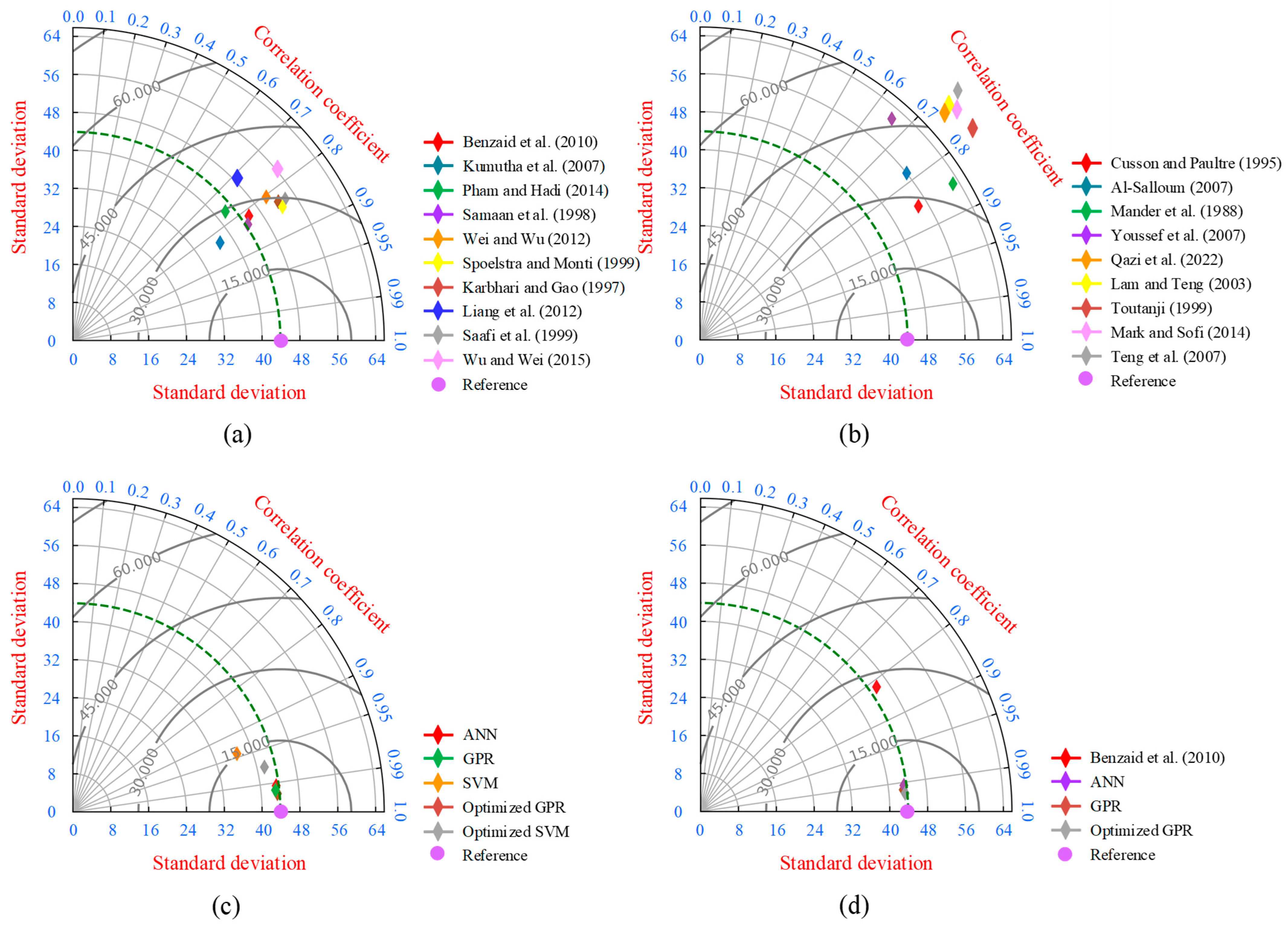
• The performance of the model of Benzaid et al. [48] was good in comparison with all other empirical models. The R and RMSE values of the model of Benzaid et al. [48] were 0.8177 and 27.02 MPa, respectively.
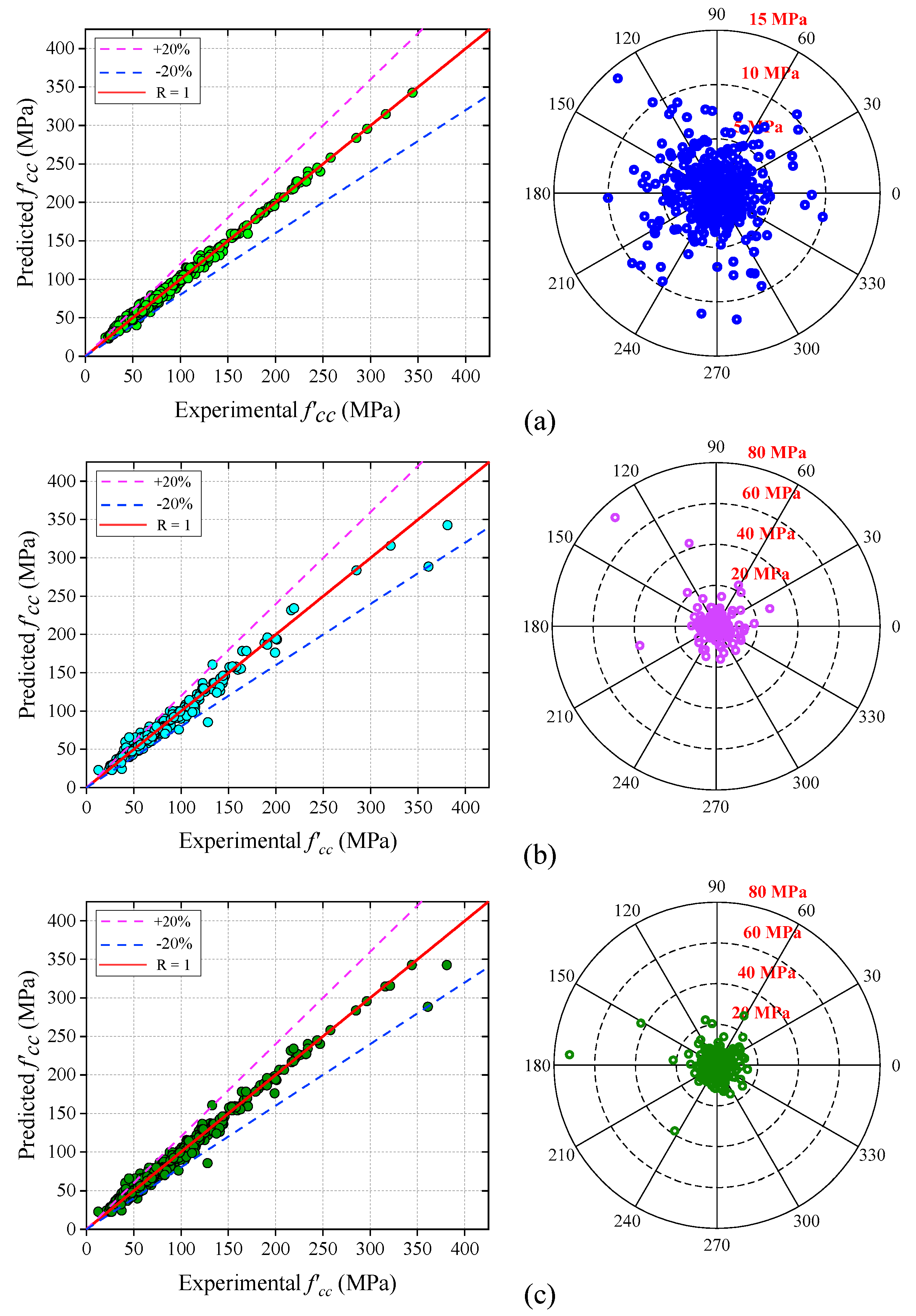
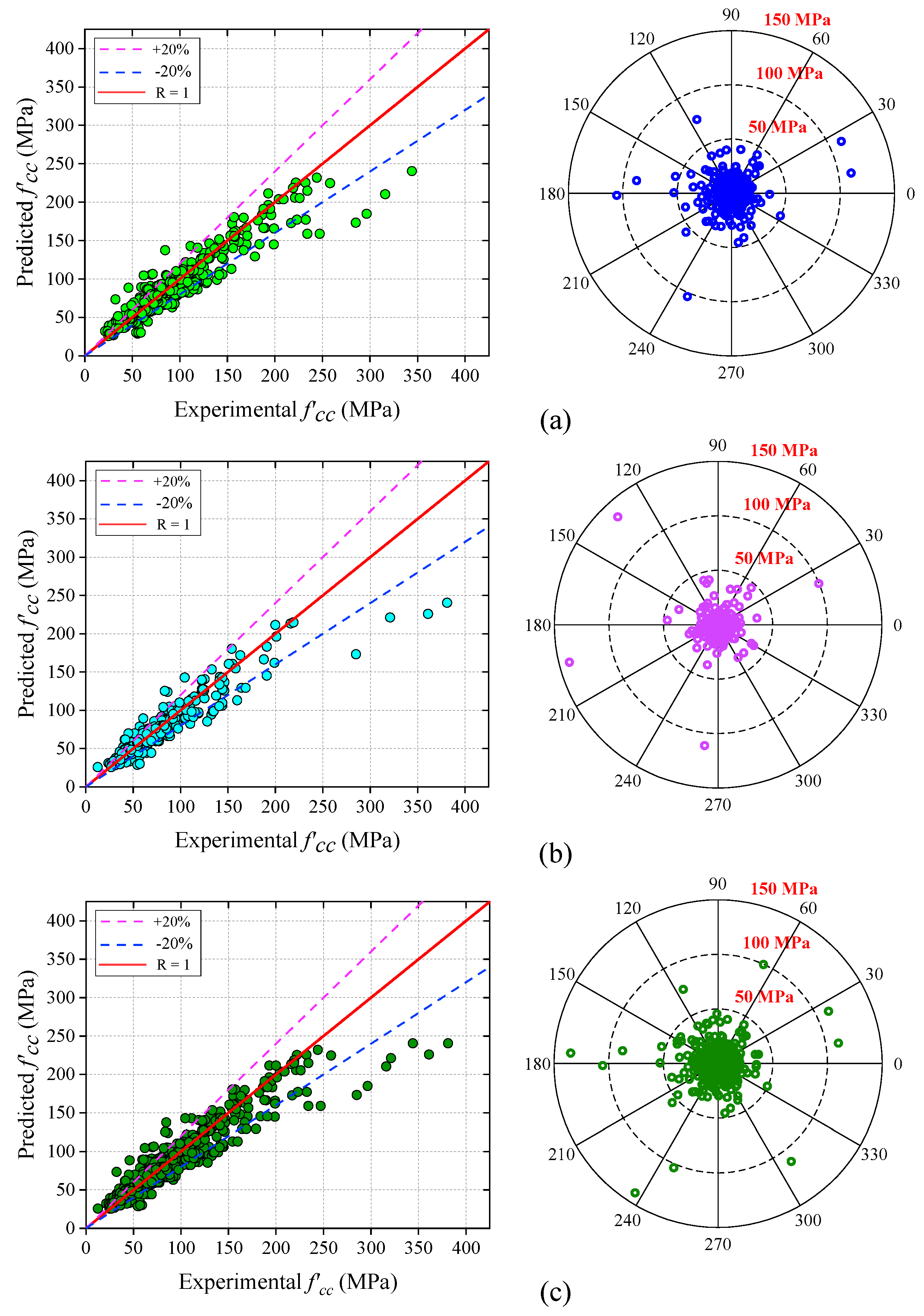
• According to the assessment criteria, the accuracy of the developed ML models decreased subsequently for the optimized GPR, GPR, ANN, optimized SVM, and SVM.
• The error values depicted by the optimized GPR model was minimum in all the cases. The MAPE, MAE, and RMSE values of the optimized GPR model were 3.11%, 2.17 MPa, and 3.88 MPa, respectively.
• By comparing the ML models and the analytical models, it was observed that the optimized GPR model reduced the error rate of MAPE, MAE, and RMSE by 727.97%, 778.34%, and 596.39%, respectively, and more accurately predicted the CS of the FRP-confined concrete cylinders than the existing mathematical models.
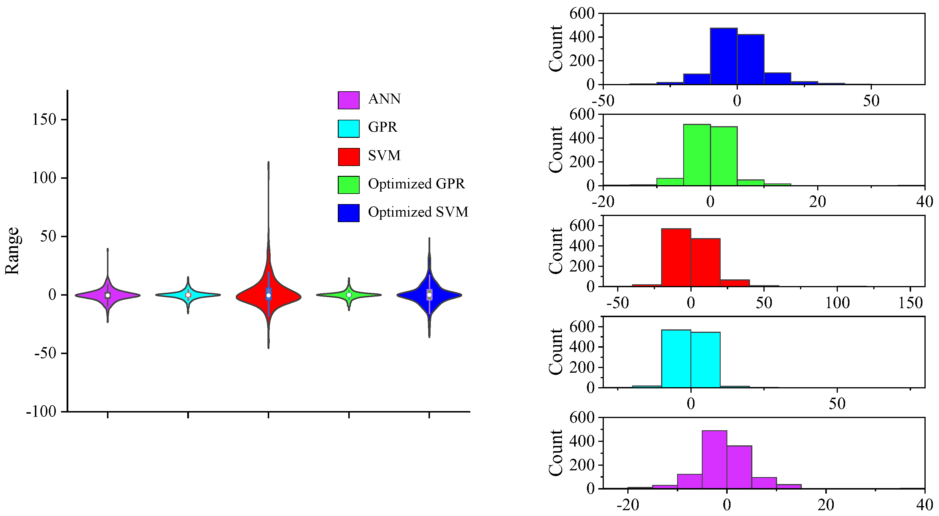
• The SVM model demonstrated a poor performance among all the ML-based models according to the performance indices, violin plot, and Taylor diagrams.
• Among all the analytical models selected in this study, the model of Teng et al. [100] illustrated poorer results with the R-value and RMSE value of 0.7200 and 67.25 MPa, respectively.

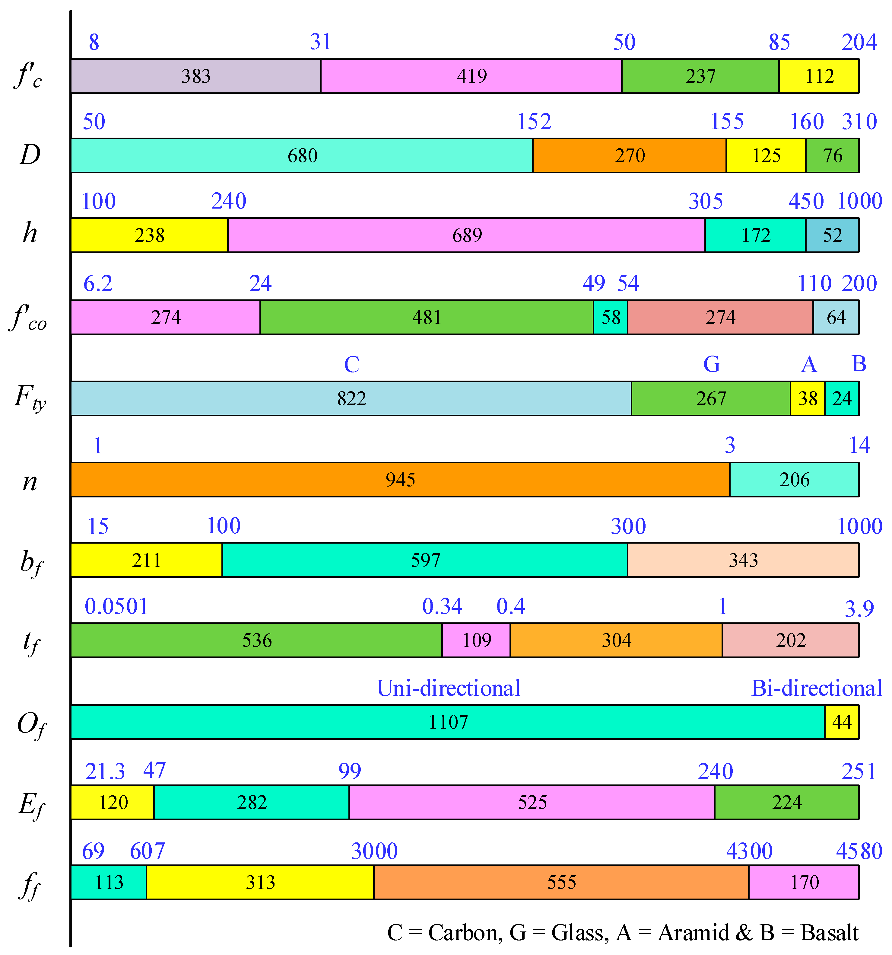
The values of input parameters should be in the range of the developed model, i.e., mentioned in Table 2. If the input parameters values are beyond the minimum and maximum range of the parameters, then the reliability of the model can be compromised, and this is the main limitation of the study. The proposed work will help the researchers, scientists, and professionals predict the CS of the FRP-confined concrete cylinders. In future works, the CS and axial capacity of the corroded FRP-confined concrete cylinders can be predicted using the ML algorithms. In addition, nature-inspired algorithms can be used to improve the precision and reliability of the predicted models.

References

1. Jung, J.S.; Lee, B.Y.; Lee, K.S. Experimental study on the structural performance degradation of corrosion-damaged reinforced concrete beams. Adv. Civ. Eng. 2019, 2019, 9562574. [Google Scholar] [CrossRef]
2. Kumar, R.; Gardoni, P. Stochastic modeling of deterioration in buildings and civil infrastructure. In Handbook of Seismic Risk Analysis and Management of Civil Infrastructure Systems, 1st ed.; Tesfamariam, S., Goda, K., Eds.; Woodhead Publishing: Cambridge, UK, 2013; pp. 410–434. [Google Scholar] [CrossRef]
3. James, A.; Bazarchi, E.; Chiniforush, A.A.; Aghdam, P.P.; Hosseini, M.R.; Akbarnezhad, A.; Martek, I.; Ghodoosi, F. Rebar corrosion detection, protection, and rehabilitation of reinforced concrete structures in coastal environments: A review. Constr. Build. Mater. 2019, 224, 1026–1039. [Google Scholar] [CrossRef]
4. Bossio, A.; Fabbrocino, F.; Monetta, T.; Lignola, G.P.; Prota, A.; Manfredi, G.; Bellucci, F. Corrosion effects on seismic capacity of reinforced concrete structures. Corros. Rev. 2019, 37, 45–56. [Google Scholar] [CrossRef]
5. Broomfield, J.P. Corrosion of Steel in Concrete: Understanding, Investigation and Repair, 1st ed.; CRC Press: London, UK, 1996; ISBN 9780429204081. [Google Scholar] [CrossRef]
6. Khan, M.U.; Ahmad, S.; Al-Gahtani, H.J. Chloride-induced corrosion of steel in concrete: An overview on chloride diffusion and prediction of corrosion initiation time. Int. J. Corros. 2017, 2017, 5819202. [Google Scholar] [CrossRef]
7. Zhou, Y.; Gencturk, B.; Willam, K.; Attar, A. Carbonation-induced and chloride-induced corrosion in reinforced concrete structures. J. Mater. Civ. Eng. 2015, 27, 04014245. [Google Scholar] [CrossRef]
8. Apostolopoulos, C.A.; Diamantogiannis, G.; Apostolopoulos, A.C. Assessment of the mechanical behavior in dual-phase steel B400C, B 450C, and B500B in a marine environment. J. Mater. Civ. Eng. 2016, 28, 04015097. [Google Scholar] [CrossRef]
9. ACI Committee. 546.3 R-14: Guide to Materials Selection for Concrete Repair; American Concrete Institute: Farmington Hills, MI, USA, 2014; ISBN 9780870318955. [Google Scholar]
10. Motavalli, M.; Czaderski, C. FRP composites for retrofitting of existing civil structures in Europe: State-of-the-art review. In Proceedings of the International Conference of Composites & Polycon, Tampa, FL, USA, 17–19 October 2007. [Google Scholar]
11. Campione, G.; Miraglia, N. Strength and strain capacities of concrete compression members reinforced with FRP. Cem. Concr. Compos. 2003, 25, 31–41. [Google Scholar] [CrossRef]
12. Sen, R. Advances in the application of FRP for repairing corrosion damage. Prog. Struct. Eng. Mater. 2003, 5, 99–113. [Google Scholar] [CrossRef]
13. Rajak, D.K.; Pagar, D.D.; Menezes, P.L.; Linul, E. Fiber-reinforced polymer composites: Manufacturing, properties, and applications. Polymers 2019, 11, 1667. [Google Scholar] [CrossRef]
14. Lee, L.S.; Jain, R. The role of FRP composites in a sustainable world. Clean Technol. Environ. Policy 2009, 11, 247–249. [Google Scholar] [CrossRef]
15. Jiang, C. Strength enhancement due to FRP confinement for coarse aggregate-free concretes. Eng. Struct. 2023, 277, 115370. [Google Scholar] [CrossRef]
16. Jiang, C.; Wu, Y.-F.; Jiang, J.-F. Effect of aggregate size on stress-strain behavior of concrete confined by fiber composites. Compos. Struct. 2017, 168, 851–862. [Google Scholar] [CrossRef]
17. Jamatia, R.; Deb, A. Size effect in FRP-confined concrete under axial compression. J. Compos. Constr. 2017, 21, 04017045. [Google Scholar] [CrossRef]
18. Khalil, M.; Ruggieri, S.; Uva, G. Assessment of structural behavior, vulnerability, and risk of industrial silos: State-of-the-art and recent research trends. Appl. Sci. 2022, 12, 3006. [Google Scholar] [CrossRef]
19. Jamatia, R.; Hussain, T.; Deb, A.; Bhattacharyya, S.K. Effect of imperfections in the bond on the strength of FRP wrapped cylindrical concrete columns. Compos. B Eng. 2013, 53, 297–307. [Google Scholar] [CrossRef]
20. Ruggieri, S.; Cardellicchio, A.; Leggieri, V.; Uva, G. Machine-learning based vulnerability analysis of existing buildings. Autom. Constr. 2021, 132, 103936. [Google Scholar] [CrossRef]
21. Hollaway, L.C. A review of the present and future utilization of FRP composites in the civil infrastructure with reference to their important in-service properties. Constr. Build. Mater. 2010, 24, 2419–2445. [Google Scholar] [CrossRef]
22. Homam, S.M.; Sheikh, S.A.; Collins, P.; Pernica, G.; Daoud, J. Durability of fiber reinforced polymers used in concrete structures. In Proceedings of the International Conference on Advanced Materials in Bridges and Structures, Ottawa, ON, Canada, 15–18 August 2000. [Google Scholar]
23. Trapko, T. Fibre Reinforced Cementitious Matrix confined concrete elements. Mater. Des. 2013, 44, 382–391. [Google Scholar] [CrossRef]
24. Kumar, A.; Arora, H.C.; Kumar, K.; Mohammed, M.A.; Majumdar, A.; Khamaksorn, A.; Thinnukool, O. Prediction of FRCM–concrete bond strength with machine learning approach. Sustainability 2022, 14, 845. [Google Scholar] [CrossRef]
25. Kumar, A.; Mor, N. An approach-driven: Use of artificial intelligence and its applications in civil engineering. In Artificial Intelligence and IoT, 1st ed.; Manoharan, K.G., Nehru, J.A., Balasubramanian, S., Eds.; Studies in Big Data; Springer: Berlin/Heidelberg, Germany, 2021; Volume 85, pp. 201–222. [Google Scholar] [CrossRef]
26. Kapoor, N.R.; Kumar, A.; Arora, H.C.; Kumar, A. Structural health monitoring of existing building structures for creating green smart cities using deep learning. In Recurrent Neural Networks, 1st ed.; Tyagi, A.K., Abraham, A., Eds.; CRC Press: Boca Raton, FL, USA, 2022; pp. 203–232. [Google Scholar] [CrossRef]
27. Kumar, K.; Saini, R.P. Adaptive neuro-fuzzy interface system-based performance monitoring technique for hydropower plants. ISH J. Hydraul. Eng. 2022, 1–11. [Google Scholar] [CrossRef]
28. Cevik, A.; Guzelbey, I.H. Neural network modeling of strength enhancement for CFRP confined concrete cylinders. Build. Environ. 2008, 43, 751–763. [Google Scholar] [CrossRef]
29. Gandomi, A.H.; Alavi, A.H.; Sahab, M.G. New formulation for compressive strength of CFRP confined concrete cylinders using linear genetic programming. Mater. Struct. 2010, 43, 963–983. [Google Scholar] [CrossRef]
30. Naderpour, H.; Kheyroddin, A.; Amiri, G.G. Prediction of FRP-confined compressive strength of concrete using artificial neural networks. Compos. Struct. 2010, 92, 2817–2829. [Google Scholar] [CrossRef]
31. Cevik, A.; Göğüş, M.T.; Güzelbey, İ.H.; Filiz, H. Soft computing-based formulation for strength enhancement of CFRP confined concrete cylinders. Adv. Eng. Softw. 2010, 41, 527–536. [Google Scholar] [CrossRef]
32. Cevik, A. Modeling strength enhancement of FRP confined concrete cylinders using soft computing. Expert Syst. Appl. 2011, 38, 5662–5673. [Google Scholar] [CrossRef]
33. Elsanadedy, H.M.; Al-Salloum, Y.A.; Abbas, H.; Alsayed, S.H. Prediction of strength parameters of FRP-confined concrete. Compos. B Eng. 2012, 43, 229–239. [Google Scholar] [CrossRef]
34. Jalal, M.; Ramezanianpour, A.A. Strength enhancement modeling of concrete cylinders confined with CFRP composites using artificial neural networks. Compos. B Eng. 2012, 43, 2990–3000. [Google Scholar] [CrossRef]
35. Pham, T.M.; Hadi, M.N. Predicting stress and strain of FRP-confined square/rectangular columns using artificial neural networks. J. Compos. Constr. 2014, 18, 04014019. [Google Scholar] [CrossRef]
36. Lim, J.C.; Karakus, M.; Ozbakkaloglu, T. Evaluation of ultimate conditions of FRP-confined concrete columns using genetic programming. Comput. Struct. 2016, 162, 28–37. [Google Scholar] [CrossRef]
37. Mansouri, I.; Kisi, O.; Sadeghian, P.; Lee, C.H.; Hu, J.W. Prediction of ultimate strain and strength of FRP-confined concrete cylinders using soft computing methods. Appl. Sci. 2017, 7, 751. [Google Scholar] [CrossRef]
38. Mozumder, R.A.; Roy, B.; Laskar, A.I. Support vector regression approach to predict the strength of FRP confined concrete. Arab. J. Sci. Eng. 2017, 42, 1129–1146. [Google Scholar] [CrossRef]
39. Kamgar, R.; Naderpour, H.; Komeleh, H.E.; Jakubczyk-Gałczyńska, A.; Jankowski, R. A proposed soft computing model for ultimate strength estimation of FRP-confined concrete cylinders. Appl. Sci. 2020, 10, 1769. [Google Scholar] [CrossRef]
40. Keshtegar, B.; Gholampour, A.; Thai, D.K.; Taylan, O.; Trung, N.T. Hybrid regression and machine learning model for predicting ultimate condition of FRP-confined concrete. Compos. Struct. 2021, 262, 113644. [Google Scholar] [CrossRef]
41. Kumar, A.; Arora, H.C.; Kapoor, N.R.; Mohammed, M.A.; Kumar, K.; Majumdar, A.; Thinnukool, O. Compressive strength prediction of lightweight concrete: Machine learning models. Sustainability 2022, 14, 2404. [Google Scholar] [CrossRef]
42. Kumar, A.; Arora, H.C.; Kapoor, N.R.; Kumar, K. Prognosis of compressive strength of fly-ash-based geopolymer-modified sustainable concrete with ML algorithms. Struct. Concr. 2022, 1–25. [Google Scholar] [CrossRef]
43. Jamali, F.; Mousavi, S.R.; Peyma, A.B.; Moodi, Y. Prediction of compressive strength of fiber-reinforced polymers-confined cylindrical concrete using artificial intelligence methods. J. Reinf. Plast. Compos. 2022, 41, 07316844211068116. [Google Scholar] [CrossRef]
44. Jalal, M.; Ramezanianpour, A.A.; Pouladkhan, A.R.; Tedro, P. Retraction Note to: Application of genetic programming (GP) and ANFIS for strength enhancement modeling of CFRP-retrofitted concrete cylinders. Neural. Comput. Appl. 2021, 33, 12245. [Google Scholar] [CrossRef]
45. Ahmad, A.; Plevris, V.; Khan, Q.U.Z. Prediction of properties of FRP-confined concrete cylinders based on artificial neural networks. Crystals 2020, 10, 811. [Google Scholar] [CrossRef]
46. Akogbe, R.K.; Liang, M.; Wu, Z.M. Size effect of axial compressive strength of CFRP confined concrete cylinders. Int. J. Concr. Struct. Mater. 2011, 5, 49–55. [Google Scholar] [CrossRef]
47. Aire, C.; Gettu, R.; Casas, J.R.; Marques, S.; Marques, D. Concrete laterally confined with fibre-reinforced polymers (FRP): Experimental study and theoretical model. Mater. Constr. 2010, 60, 19–31. [Google Scholar] [CrossRef]
48. Benzaid, R.; Mesbah, H.; Chikh, N.E. FRP-confined concrete cylinders: Axial compression experiments and strength model. J. Reinf. Plast. Compos. 2010, 29, 2469–2488. [Google Scholar] [CrossRef]
49. Berthet, J.F.; Ferrier, E.; Hamelin, P. Compressive behavior of concrete externally confined by composite jackets. Part A: Experimental study. Constr. Build. Mater. 2005, 19, 223–232. [Google Scholar] [CrossRef]
50. Carey, S.A.; Harries, K.A. Axial behavior and modeling of confined small-, medium-, and large-scale circular sections with carbon fiber-reinforced polymer jackets. ACI Struct. J. 2005, 102, 596. [Google Scholar] [CrossRef]
51. Demers, M.; Neale, K.W. Confinement of reinforced concrete columns with fiber-reinforced composite sheets—An experimental study. Can. J. Civ. Eng. 1999, 26, 226–241. [Google Scholar] [CrossRef]
52. Elsanadedy, H.M.; Al-Salloum, Y.A.; Alsayed, S.H.; Iqbal, R.A. Experimental and numerical investigation of size effects in FRP-wrapped concrete columns. Constr. Build. Mater. 2012, 29, 56–72. [Google Scholar] [CrossRef]
53. Erdil, B.; Akyuz, U.; Yaman, I.O. Mechanical behavior of CFRP confined low strength concretes subjected to simultaneous heating–cooling cycles and sustained loading. Mater. Struct. 2012, 45, 223–233. [Google Scholar] [CrossRef]
54. Ilki, A.; Kumbasar, N.; Koc, V. Strength and deformability of low strength concrete confined by carbon fiber composite sheets. In Proceedings of the ASCE 15th Engineering Mechanics Conference, Columbia University, New York, NY, USA, 2–5 June 2002. [Google Scholar]
55. Karabinis, A.I.; Rousakis, T.C. Concrete confined by FRP material: A plasticity approach. Eng. Struct. 2002, 24, 923–932. [Google Scholar] [CrossRef]
56. Lee, J.Y.; Yi, C.K.; Jeong, H.S.; Kim, S.W.; Kim, J.K. Compressive response of concrete confined with steel spirals and FRP composites. J. Compos. Mater. 2010, 44, 481–504. [Google Scholar] [CrossRef]
57. Lin, C.T.; Li, Y.F. An effective peak stress formula for concrete confined with carbon fiber reinforced plastics. Can. J. Civ. Eng. 2003, 30, 882–889. [Google Scholar] [CrossRef]
58. Liang, M.; Wu, Z.M.; Ueda, T.; Zheng, J.J.; Akogbe, R. Experiment and modeling on axial behavior of carbon fiber reinforced polymer confined concrete cylinders with different sizes. J. Reinf. Plast. Compos. 2012, 31, 389–403. [Google Scholar] [CrossRef]
59. Mandal, S.; Hoskin, A.; Fam, A. Influence of concrete strength on confinement effectiveness of fiber-reinforced polymer circular jackets. ACI Struct. J. 2005, 102, 383. [Google Scholar] [CrossRef]
60. Song, X.; Gu, X.; Li, Y.; Chen, T.; Zhang, W. Mechanical behavior of FRP-strengthened concrete columns subjected to concentric and eccentric compression loading. J. Compos. Constr. 2013, 17, 336–346. [Google Scholar] [CrossRef]
61. Shehata, I.A.; Carneiro, L.A.; Shehata, L.C. Strength of short concrete columns confined with CFRP sheets. Mat. Struct. 2002, 35, 50–58. [Google Scholar] [CrossRef]
62. Valdmanis, V.; De Lorenzis, L.; Rousakis, T.; Tepfers, R. Behaviour and capacity of CFRP-confined concrete cylinders subjected to monotonic and cyclic axial compressive load. Struct. Concr. 2007, 8, 187–200. [Google Scholar] [CrossRef]
63. Vincent, T.; Ozbakkaloglu, T. Influence of concrete strength and confinement method on axial compressive behavior of FRP confined high-and ultra-high-strength concrete. Compos. B Eng. 2013, 50, 413–428. [Google Scholar] [CrossRef]
64. Shahawy, M.; Mirmiran, A.; Beitelman, T. Tests and modeling of carbon-wrapped concrete columns. Compos. B Eng. 2000, 31, 471–480. [Google Scholar] [CrossRef]
65. Wu, Y.F.; Jiang, J.F. Effective strain of FRP for confined circular concrete columns. Compos. Struct. 2013, 95, 479–491. [Google Scholar] [CrossRef]
66. Shao, Y.; Zhu, Z.; Mirmiran, A. Cyclic modeling of FRP-confined concrete with improved ductility. Cem. Concr. Compos. 2006, 28, 959–968. [Google Scholar] [CrossRef]
67. Silva, M.A.; Rodrigues, C.C. Size and relative stiffness effects on compressive failure of concrete columns wrapped with glass FRP. J. Mater. Civ. Eng. 2006, 18, 334–342. [Google Scholar] [CrossRef]
68. Comert, M.; Goksu, C.; Ilki, A. Towards a tailored stress-strain behavior for FRP confined low strength concrete. In Proceedings of the 9th International Symposium on Fiber Reinforced Polymer Reinforcement for Concrete Structures, Sydney, Australia, 13–15 July 2009. [Google Scholar]
69. Mirmiran, A.; Shahawy, M.; Samaan, M.; Echary, H.E.; Mastrapa, J.C.; Pico, O. Effect of column parameters on FRP-confined concrete. J. Compos. Constr. 1998, 2, 175–185. [Google Scholar] [CrossRef]
70. Li, G.; Maricherla, D.; Singh, K.; Pang, S.S.; John, M. Effect of fiber orientation on the structural behavior of FRP wrapped concrete cylinders. Compos. Struct. 2006, 74, 475–483. [Google Scholar] [CrossRef]
71. De Oliveira, D.S.; Raiz, V.; Carrazedo, R. Experimental study on normal-strength, high-strength and ultrahigh-strength concrete confined by carbon and glass FRP laminates. J. Compos. Constr. 2019, 23, 04018072. [Google Scholar] [CrossRef]
72. Touhari, M.; Mitiche-Kettab, R. Behaviour of FRP confined concrete cylinders: Experimental investigation and strength model. Period. Polytech. Civ. Eng. 2016, 60, 647–660. [Google Scholar] [CrossRef]
73. Almusallam, T.H. Behavior of normal and high-strength concrete cylinders confined with E-glass/epoxy composite laminates. Compos. B Eng. 2007, 38, 629–639. [Google Scholar] [CrossRef]
74. Sadeghian, P.; Fillmore, B. Strain distribution of basalt FRP-wrapped concrete cylinders. Case Stud. Constr. Mater. 2018, 9, e00171. [Google Scholar] [CrossRef]
75. Ma, G.; Chen, X.; Yan, L.; Hwang, H.J. Monotonic and cyclic axial compressive properties and modeling of basalt FRP-retrofitted predamaged short columns. J. Compos. Constr. 2020, 24, 04020023. [Google Scholar] [CrossRef]
76. Ilki, A.; Peker, O.; Karamuk, E.; Demir, C.; Kumbasar, N. FRP retrofit of low and medium strength circular and rectangular reinforced concrete columns. J. Mater. Civ. Eng. 2008, 20, 169–188. [Google Scholar] [CrossRef]
77. Eid, R.; Roy, N.; Paultre, P. Normal-and high-strength concrete circular elements wrapped with FRP composites. J. Compos. Constr. 2009, 13, 113–124. [Google Scholar] [CrossRef]
78. Micelli, F.; Myers, J.J. Durability of FRP-confined concrete. Proc. Inst. Civ. Eng. Constr. Mater. 2008, 161, 173–185. [Google Scholar] [CrossRef]
79. Aire, C.; Gettu, R.; Casas, J.R. Study of the compressive behavior of concrete confined by fiber reinforced composites. In Proceedings of the CCC 2001—International Conference on Composites in Construction, Porto, Portugal, 10–12 October 2001. [Google Scholar]
80. Zeng, J.J.; Guo, Y.C.; Gao, W.Y.; Chen, W.P.; Li, L.J. Stress-strain behavior of concrete in circular concrete columns partially wrapped with FRP strips. Compos. Struct. 2018, 200, 810–828. [Google Scholar] [CrossRef]
81. Kaeseberg, S.; Messerer, D.; Holschemacher, K. Experimental study on concrete under combined FRP–Steel confinement. Materials 2020, 13, 4467. [Google Scholar] [CrossRef]
82. Ghernouti, Y.; Rabehi, B. FRP-confined short concrete columns under compressive loading: Experimental and modeling investigation. J. Reinf. Plast. Compos. 2011, 30, 241–255. [Google Scholar] [CrossRef]
83. Ozbakkaloglu, T.; Vincent, T. Axial compressive behavior of circular high-strength concrete-filled FRP tubes. J. Compos. Constr. 2014, 18, 04013037. [Google Scholar] [CrossRef]
84. Abdollahi, B.; Bakhshi, M.; Mirzaee, Z.; Shekarchi, M.; Motavalli, M. SIFCON strengthening of concrete cylinders in comparison with conventional GFRP confinement method. Constr. Build. Mater. 2012, 36, 765–778. [Google Scholar] [CrossRef]
85. Park, J.H.; Jo, B.W.; Yoon, S.J.; Park, S.K. Experimental investigation on the structural behavior of concrete filled FRP tubes with/without steel re-bar. KSCE J. Civ. Eng. 2011, 15, 337–345. [Google Scholar] [CrossRef]
86. Ozbakkaloglu, T.; Akin, E. Behavior of FRP-confined normal-and high-strength concrete under cyclic axial compression. J. Compos. Constr. 2012, 16, 451–463. [Google Scholar] [CrossRef]
87. Zhou, J.; Bi, F.; Wang, Z.; Zhang, J. Experimental investigation of size effect on mechanical properties of carbon fiber reinforced polymer (CFRP) confined concrete circular specimens. Constr. Build. Mater. 2016, 127, 643–652. [Google Scholar] [CrossRef]
88. Li, P.; Wu, Y.F.; Gravina, R. Cyclic response of FRP-confined concrete with post-peak strain softening behavior. Constr. Build. Mater. 2016, 123, 814–828. [Google Scholar] [CrossRef]
89. Saeed, H.Z.; Khan, H.A.; Farooq, R. Experimental investigation of stress–strain behavior of CFRP confined Low Strength Concrete (LSC) cylinders. Constr. Build. Mater. 2016, 104, 208–215. [Google Scholar] [CrossRef]
90. Kapoor, N.R.; Kumar, A.; Kumar, A.; Kumar, A.; Mohammed, M.A.; Kumar, K.; Kadry, S.; Lim, S. Machine learning-based CO2 prediction for office room: A pilot study. Wirel. Commun. Mob. Comput. 2022, 2022, 9404807. [Google Scholar] [CrossRef]
91. Kumar, A.; Arora, H.C.; Mohammed, M.A.; Kumar, K.; Nedoma, J. An optimized neuro-bee algorithm approach to predict the FRP-concrete bond strength of RC beams. IEEE Access 2021, 10, 3790–3806. [Google Scholar] [CrossRef]
92. Wu, Y.F.; Wei, Y. General stress-strain model for steel-and FRP-confined concrete. J. Compos. Constr. 2015, 19, 04014069. [Google Scholar] [CrossRef]
93. Pham, T.M.; Hadi, M.N. Confinement model for FRP confined normal-and high-strength concrete circular columns. Constr. Build. Mater. 2014, 69, 83–90. [Google Scholar] [CrossRef]
94. Youssef, M.N.; Feng, M.Q.; Mosallam, A.S. Stress–strain model for concrete confined by FRP composites. Compos. B Eng. 2007, 38, 614–628. [Google Scholar] [CrossRef]
95. Kumutha, R.; Vaidyanathan, R.; Palanichamy, M.S. Behaviour of reinforced concrete rectangular columns strengthened using GFRP. Cem. Concr. Compos. 2007, 29, 609–615. [Google Scholar] [CrossRef]
96. Samaan, M.; Mirmiran, A.; Shahawy, M. Model of concrete confined by fiber composites. J. Struct. Eng. 1998, 124, 1025–1031. [Google Scholar] [CrossRef]
97. Toutanji, H. Stress-strain characteristics of concrete columns externally confined with advanced fiber composite sheets. Mater. J. 1999, 96, 397–404. [Google Scholar] [CrossRef]
98. Wei, Y.Y.; Wu, Y.F. Unified stress–strain model of concrete for FRP-confined columns. Constr. Build. Mater. 2012, 26, 381–392. [Google Scholar] [CrossRef]
99. Saafi, M.; Toutanji, H.; Li, Z. Behavior of concrete columns confined with fiber reinforced polymer tubes. Mater. J. 1999, 96, 500–509. [Google Scholar] [CrossRef]
100. Teng, J.; Huang, Y.L.; Lam, L.; Ye, L.P. Theoretical model for fiber-reinforced polymer-confined concrete. J. Compos. Constr. 2007, 11, 201–210. [Google Scholar] [CrossRef]
101. Mander, J.B.; Priestley, M.J.; Park, R. Theoretical stress-strain model for confined concrete. J. Struct. Eng. 1988, 114, 1804–1826. [Google Scholar] [CrossRef]
102. Spoelstra, M.R.; Monti, G. FRP-confined concrete model. J. Compos. Constr. 1999, 3, 143–150. [Google Scholar] [CrossRef]
103. Mark, A.R.A.; Sofi, A. GFRP confined concrete under uni-axial loading. Singap. J. Sci. Res. 2014, 6, 72–75. [Google Scholar]
104. Karbhari, V.M.; Gao, Y. Composite jacketed concrete under uniaxial compression—Verification of simple design equations. J. Mater. Civ. Eng. 1997, 9, 185–193. [Google Scholar] [CrossRef]
105. Lam, L.; Teng, J.G. Design-oriented stress–strain model for FRP-confined concrete. Constr. Build. Mater. 2003, 17, 471–489. [Google Scholar] [CrossRef]
106. Cusson, D.; Paultre, P. Stress-strain model for confined high-strength concrete. J. Struct. Eng. 1995, 121, 468–477. [Google Scholar] [CrossRef]
107. Al-Salloum, Y.A. Compressive strength models of FRP-confined concrete. In Proceedings of the Asia-Pacific Conference on FRP in Structures (APFIS 2007), Hong Kong, China, 12–14 December 2007. [Google Scholar]
108. Qazi, A.U.; Khan, Q.S.; Ahmad, H.A.; Pham, T.M. Axial behavior of FRP confined concrete using locally available low-cost wraps. Sustainability 2022, 14, 9989. [Google Scholar] [CrossRef]
109. Zakaria, M.; Al-Shebany, M.; Sarhan, S. Artificial neural network: A brief overview. Int. J. Eng. Res. Appl. 2014, 4, 7–12. [Google Scholar]
110. Han, S.H.; Kim, K.W.; Kim, S.; Youn, Y.C. Artificial neural network: Understanding the basic concepts without mathematics. Dement. Neurocogn. Disord. 2018, 17, 83–89. [Google Scholar] [CrossRef]
111. Dongare, A.D.; Kharde, R.R.; Kachare, A.D. Introduction to artificial neural network. Int. J. Eng. Innov. Technol. 2012, 2, 189–194. [Google Scholar]
112. Jain, A.K.; Mao, J.; Mohiuddin, K.M. Artificial neural networks: A tutorial. Computer 1996, 29, 31–44. [Google Scholar] [CrossRef]
113. Ouaer, H.; Hosseini, A.H.; Nait Amar, M.; El Amine Ben Seghier, M.; Ghriga, M.A.; Nabipour, N.; Andersen, P.Ø.; Mosavi, A.; Shamshirband, S. Rigorous connectionist models to predict carbon dioxide solubility in various ionic liquids. Appl. Sci. 2019, 10, 304. [Google Scholar] [CrossRef]
114. Asante-Okyere, S.; Shen, C.; Yevenyo Ziggah, Y.; Moses Rulegeya, M.; Zhu, X. Investigating the predictive performance of Gaussian process regression in evaluating reservoir porosity and permeability. Energies 2018, 11, 3261. [Google Scholar] [CrossRef]
115. Cheng, L.; Ramchandran, S.; Vatanen, T.; Lietzén, N.; Lahesmaa, R.; Vehtari, A.; Lähdesmäki, H. An additive Gaussian process regression model for interpretable non-parametric analysis of longitudinal data. Nat. Commun. 2019, 10, 1798. [Google Scholar] [CrossRef]
116. Singh, R.; Arora, H.C.; Bahrami, A.; Kumar, A.; Kapoor, N.R.; Kumar, K.; Rai, H.S. Enhancing sustainability of corroded RC structures: Estimating steel-to-concrete bond strength with ANN and SVM algorithms. Materials 2022, 15, 8295. [Google Scholar] [CrossRef] [PubMed]
117. Vapnik, V.; Golowich, S.; Smola, A. Support vector method for function approximation, regression estimation and signal processing. Adv. Neural Inf. Process. Syst. 1996, 9, 281–287. [Google Scholar]
118. Farfani, H.A.; Behnamfar, F.; Fathollahi, A. Dynamic analysis of soil-structure interaction using the neural networks and the support vector machines. Expert Syst. Appl. 2015, 42, 8971–8981. [Google Scholar] [CrossRef]
Figure 1. Details of input parameters.
Buildings 13 00931 g001
Figure 2. Heat plot of input and output parameters.
Buildings 13 00931 g002
Figure 4. Architecture of ML models (a) ANN, (b) GPR, (c) SVM.
Buildings 13 00931 g004
Figure 5. Optimized GPR.
Buildings 13 00931 g005
Figure 6. Optimized SVM.
Buildings 13 00931 g006
Figure 7. Scatter plot of analytical models; (a) Wu and Wei [92], (b) Pham and Hadi [93], (c) Youssef et al. [94], (d) Kumutha et al. [95], (e) Samaan et al. [96], (f) Toutanji [97], (g) Wei and Wu [98], (h) Saafi et al. [99], (i) Teng et al. [100], (j) Mander et al. [101], (k) Spoelstra and Monti [102], (l) Mark and Sofi [103], (m) Karbhari and Gao [104], (n) Lam and Teng [105], (o) Cusson and Paultre [106], (p) Liang et al. [58], (q) Benzaid et al. [48], (r) Al-Salloum [107], and (s) Qazi et al. [108].
Buildings 13 00931 g007aBuildings 13 00931 g007b
Figure 8. Scatter and absolute error plot of ANN model; (a) training, (b) validation, (c) testing, and (d) whole datasets.
Buildings 13 00931 g008
Figure 9. Scatter and absolute error plot of GPR model; (a) training, (b) testing, and (c) whole datasets.
Buildings 13 00931 g009
Figure 10. Scatter and absolute error plot of SVM model; (a) training, (b) testing, and (c) whole datasets.
Buildings 13 00931 g010
Figure 11. Scatter and absolute error plot of optimized GPR model; (a) training, (b) testing, and (c) whole datasets.
Buildings 13 00931 g011
Figure 12. Scatter and absolute error plot of optimized SVM model; (a) training, (b) testing, and (c) whole datasets.
Buildings 13 00931 g012
Figure 13. Violin with box plot and frequency distribution of errors.
Buildings 13 00931 g013
Figure 14. Taylor plot; (a) analytical models 1 to 10 (Benzaid et al. [48], Kumutha et al. [95], Pham and Hadi [93], Samaan et al. [96], Wei and Wu [98], Spoelstra and Monti [102], Karbhari and Gao [104], Liang et al. [58], Saafi et al. [99], Wu and Wei [92]), (b) analytical models 11 to 19 (Cusson and Paultre [106], Al-Salloum [107], Mander et al. [101], Youssef et al. [94], Qazi et al. [108], Lam and Teng [105], Toutanji [97], Mark and Sofi [103], Teng et al. [100]), (c) proposed ML models (ANN, GPR, SVM, optimized GPR, and optimized SVM models), and (d) comparison between best analytical models and best fitted ML models (Benzaid et al. [48]).
Buildings 13 00931 g014