1. Introduction
Indoor thermal comfort is vital for ensuring the well-being and productivity of the people living, working, and learning in indoor spaces. An average person is estimated to spend over 90% of their time in the built environment such as homes, offices, and schools [
1]. Therefore, indoor thermal comfort has an immense influence on the physical and emotional health, performance, and decision-making process of an occupant [
2]. However, thermal comfort perception is highly subjective and personal. An occupant evaluates and responds to the thermal environment based on factors and processes that are unique to the occupant, e.g., metabolism, temperature preference, and adaptive behavior.
Furthermore, thermal comfort (TC) is a multidimensional paradigm, which involves various contexts of an occupant’s subjective perception of the built environment. This includes sensation or feeling, temperature preference, satisfaction with indoor temperature, acceptability of the indoor thermal environment, and overall comfort level. Given the inherent subjectivity in individual perception, these contexts need to be quantified to reliably measure, estimate, and predict occupant TC. Thus, the aspects described above are represented through TC metrics, viz., Thermal Sensation Vote (TSV), Thermal Preference Vote (TPV), Thermal Acceptability (TA), Thermal Satisfaction Level (TSL), and Thermal Comfort Vote (TCV).
The use of multiple subjective TC metric responses helps create a comprehensive view of an individual’s perception in conventional TC estimation models such as the Predicted Mean Vote (PMV) model [
3] and the Adaptive model (ATC) [
4]. However, the focus of thermal comfort research in the built environment has recently shifted from conventional estimation to artificial intelligence and machine-learning (AI/ML)-based prediction. Additionally, complex and effective algorithms integrated with BIM and IoT are employed to precisely predict thermal comfort [
5], and energy usage under various design variables and parameters [
6]. Thermal comfort prediction models that leverage AI/ML have been repeatedly demonstrated to far outperform the conventional PMV and ATC models with respect to model accuracy when compared to ground truth [
7,
8,
9]. AI algorithms are capable of solving complex multi-class classification problems suitable for TC prediction. This is because AI/ML models learn multidimensional nonlinear mappings between numerous inputs (features) including building, environmental, and weather and the subjective TC metric responses of occupants.
Although AI-based predictive modeling is highly effective, the presence of multiple TC metrics creates a fresh set of challenges in accurate thermal comfort prediction. The subjective perception of an occupant may vary for different TC metrics. For example, someone may feel a sensation of “Neutral” but still prefer a “Warmer” temperature instead of “No Change” in the temperature. The problem assumes greater complexity for children such as primary school students in naturally ventilated buildings, with limited cognitive abilities [
10,
11] to evaluate their thermal comfort [
12,
13].
The existence of multiple TC metrics and incongruence in occupant responses makes TC prediction extremely challenging. The majority of current TC prediction works employ
Single Task Learning, where one AI model specifically predicts a single TC metric, leading to multiple independent TC prediction models for the same built space such as a classroom or apartment [
9].
2. Motivation and Research Problems
This work aims to address a fundamental challenge in Machine-Learning-based Thermal Comfort Studies (MLTC), i.e., the dilemma of selecting a model label/output from multiple subjective thermal comfort metrics gathered from surveys. Gathering a large number of responses on multiple TCMs may seem desirable but presents several challenges, especially when participants are primary school students [
14,
15].
First, a large number of questions causes intrusion and discourages enthusiastic participation as the study progresses. Children in particular tend to become bored when asked to fill out the same lengthy questionnaires/surveys with questions that seem repetitive to them [
16]. There is also evidence to suggest that children are more likely to become distracted, leading to a higher rate of anomalous responses [
14,
17], lowering the overall prediction accuracy of thermal comfort models. More importantly, primary school children are in the early stages of cognitive development. Therefore, multiple questions seeking subjective feedback will require a child participant to make repeated value judgments, increasing the chances of confusion and error [
18]. It is conceivable that short and straightforward questions will typically yield better response rates than lengthy questionnaires [
14,
19]. Thus, it makes sense to have fewer questions to avoid fatigue to the students [
10,
19].
The objective of this study is to explore how to evaluate subjective thermal experience with a minimal number of thermal metrics or select the most effective single TC measure. Which thermal comfort criteria should be employed to gather occupants’ assessments of their indoor thermal environment? In particular, the objective is to explore if thermal sensation (TSV), preference (TPV), comfort (TCV), acceptability (TA), and satisfaction levels (TSL) can predict all other metrics of subjective experience of thermal conditions with high accuracy.
Thermal Comfort Metrics
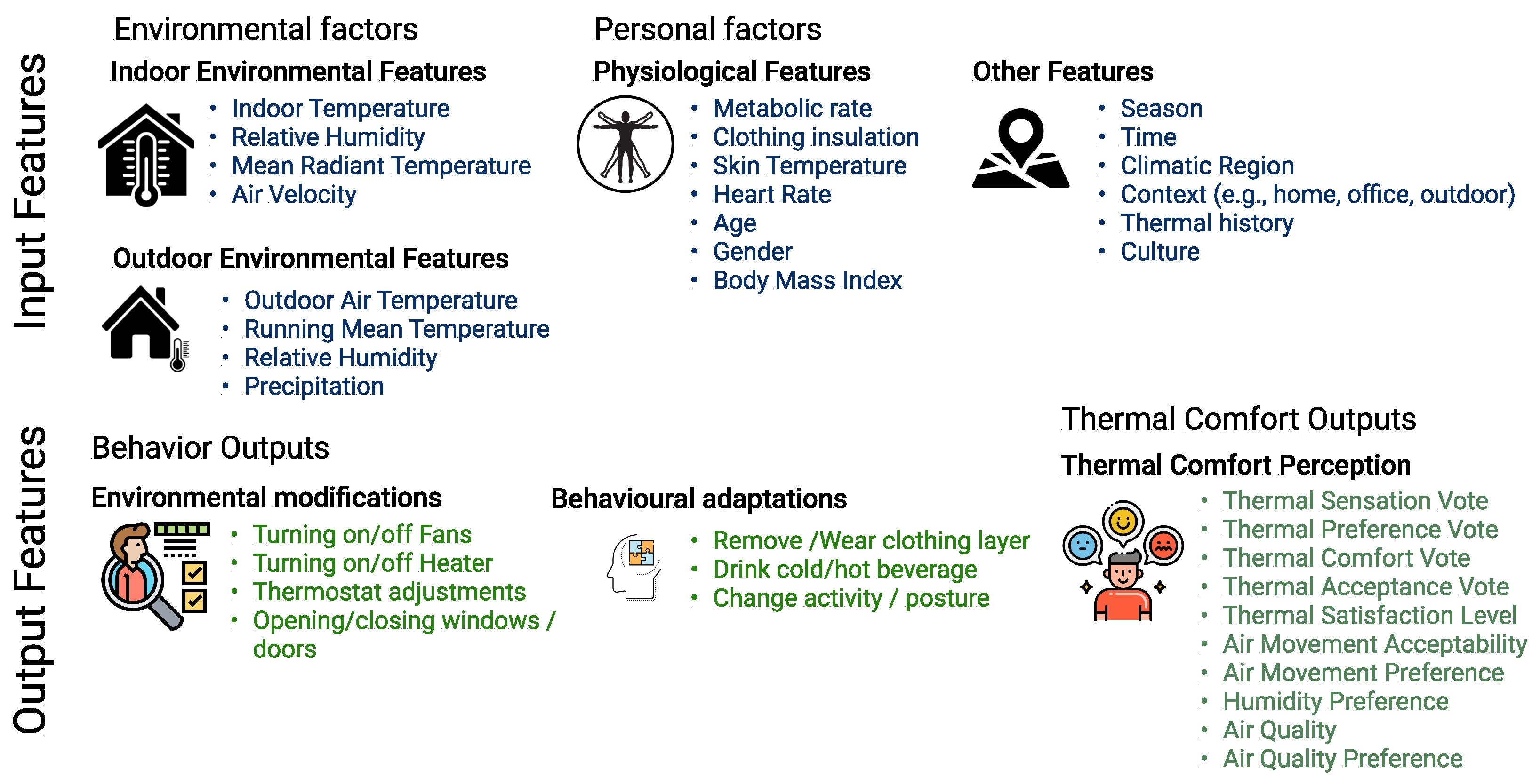
According to the ISO 7730 and ASHRAE standards, thermal comfort for an occupant can be predicted based on the physical measurement of environmental factors and personal factors, usually categorized as input parameters. Environmental assessments include measurements of air temperature (indoor and outdoor), mean radiant temperature, relative humidity, air speed (indoor) and precipitation (outdoor). Personal factors include the degree of clothing insulation, and physical activity (metabolic rate). Other input parameters include physiological factors such as age, gender, BMI, skin temperature, etc. Thermal comfort is a state of mind—a sensory experience that is assessed by subjective questionnaires. To understand the set of conditions that satisfy an occupant, the feedback collected from questionnaires can be categorized as thermal sensation vote (TSV), thermal preference vote (TPV), thermal comfort vote (TCV), thermal satisfaction (TSL), thermal acceptability (TA), humidity preferences, etc. Collectively, they can be categorized as output parameters.
Figure 1 illustrates the subjective input features (environmental and personal factors) and output parameters (adaptations and thermal comfort indices) used in various thermal comfort studies.
TSV (Thermal Sensation Vote) is most frequently used in research of subjective thermal comfort [
20]. Thermal sensation indicates how the occupant feels thermally, such as feeling “warm” or “slightly cold”, and is typically directly associated with actual measurements of temperature (indoor or outdoor). Various researchers have used different scales to assess aspects of thermal sensation depending on the survey context and age of participants.
TPV (Thermal Preference Vote) corresponds to how the occupant would prefer to adjust their thermal environment and is a better measure of what an ideal environment would be as it suggests a change from the current conditions. Therefore, TPV is often used as an effective measure to help in the prediction of HVAC systems and optimize energy efficiency [
21]. Furthermore, it is also considered to be the most interpretable indicator among the other thermal comfort metrics [
22]. TA (Thermal acceptability) determines whether the occupant accepts the current thermal conditions or not. Although “acceptability” is ideal, it is not equated with “comfort” since an occupant may not feel comfortable yet still accept the environment [
23]. Thermal Satisfaction Level (TSL) describes the occupant satisfaction with the temperature and is measured by a seven-point Likert scale, based on the ASHRAE PMV survey, ranging from −3 to +3 (Very Dissatisfied to Very Satisfied).
3. Thermal Comfort Models and ASHRAE Datasets
3.1. Thermal Comfort Models
ASHRAE Standard 55 [
24] and EN 15251, 2012 [
25] adopted the first thermal comfort model developed from climate chamber experiments by Ole Fanger [
3]. The Predictive Mean Vote (PMV) is the most recognized thermal comfort model, and it predicts the thermal sensation of a group of people within a similar thermal environment. It uses a seven-point scale and is calculated as a function of indoor air temperature, mean radiant temperature, relative humidity, air velocity, metabolic rate and value of clothing insulation. Predicted Percentage Dissatisfaction (PPD) estimates the percentage of people who would be dissatisfied in such an environment and is calculated as a function of PMV. Both PMV-PPD was developed under static state conditions, and based on principles of heat balance.
On the contrary, the adaptive thermal comfort model (ATC), another framework used to evaluate a thermal environment, is based on the concept that occupants dynamically interact with their environment [
4]. ATC predicts thermal comfort on the understanding that occupants adapt themselves according to their environment and can prefer wider adaptive opportunities in various indoor conditions. The indoor temperature and outdoor temperature correlation is analyzed through correlation coefficients and scatter plots.
However, the recent technological advances in data science such as artificial intelligence and machine-learning techniques have facilitated improved methods to predict thermal comfort by data-driven method, as compared to the previous conventional approaches. Furthermore, current machine-learning techniques have proved to be more accurate than regression tools in estimating non-standard nonlinear relations between independent and dependent variables [
23]. Random Forest, Classification Tree, Support Vector Machine, Neural Network and Bayesian network are some of the ML techniques applied in thermal comfort studies to predict TSV, TPV, TCV and TA [
7,
8,
11,
26,
27,
28].
3.2. ASHRAE Global Thermal Comfort Database II
The ASHRAE Global Thermal Comfort Database II project consists of 52 data files from 160 buildings in 28 countries, conducted between 1995 and 2016. It records over 50 features such as demographic information of subjects (sex, age, height, and weight), ‘right-now-right-here’ subjective evaluations (sensation, acceptability, and preference), the basic identifiers (year of survey, building code, location and heating/cooling strategy), and comfort indices (PMV, PPD and SET) beside instrumental measurements of indoor temperatures, air velocity, relative humidity and outdoor meteorological information.
This open-sourced organized dataset, comprising 107,463 responses, presents a unique opportunity to apply machine-learning techniques to overcome the challenges faced by existing comfort models.
4. Primary Student Survey: Description and Analysis
In addition to the data gathered from the ASHRAE Database II, the current study also looks at data gathered from the field studies carried out in India. The dataset for students is compiled from primary school surveys conducted during the summer and winter in Dehradun, India [
29]. Questions were designed to inquire about student TSV, TPV, TCV, and TA along with their satisfaction with the indoor environment (TSL) and their satisfaction with the amount of clothing insulation (SwC). Since the adaptive opportunities for students to adjust themselves to their indoor environment were limited [
29], satisfaction with clothing (SwC) was asked to comprehend if students were satisfied with their clothing and if they modified the layers of clothing to adjust their thermal conditions. The question inquired if students felt they were wearing more layers than they want, were satisfied with their current clothing layer, or if they were wearing less than they would want.
4.1. Students Thermal Responses during Winter Surveys
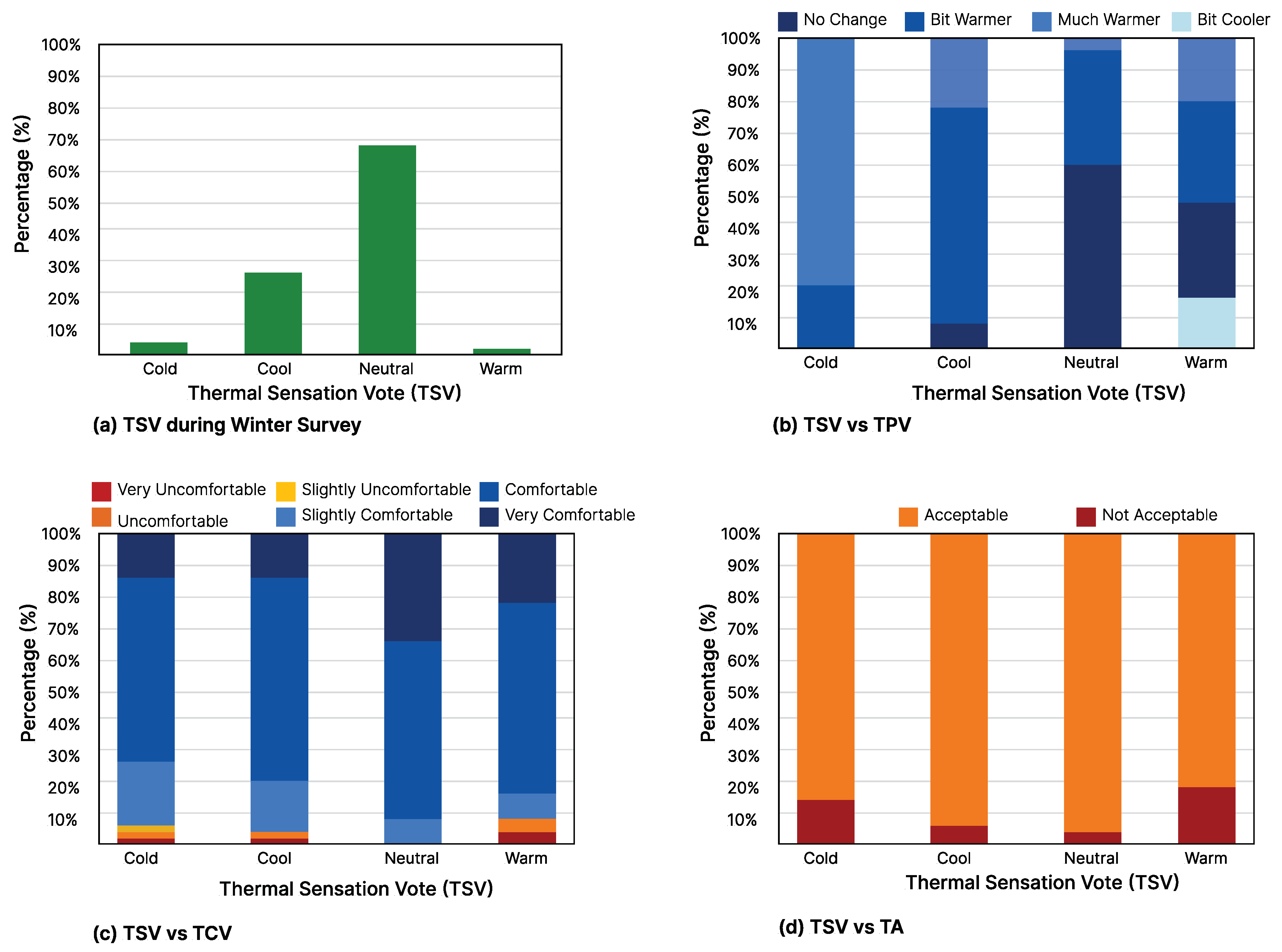
A total of 2039 responses were collected during a month-long field survey during the winter. The frequency of the students’ thermal votes is summarized in
Figure 2. As observed in
Figure 2a, regarding TSV, a maximum cluster of votes lie in the neutral TSV = 0 category with 69% votes. The rest of the TSV is distributed between feeling cold (TSV = −2) 4%, cool (TSV = 1) 23% and surprisingly 2% of the students feel warm (TSV = 1).
Figure 2b shows 57% of students prefer a warmer indoor environment (TPV = 1, 2) and 43% prefer no change (TPV = 0). Students were also found to be comfortable (TCV = 1, 2, 3 = 98%) and satisfied (TSL = 1, 2, 3 = 97%) with their classroom environment. In addition, 96% students found the classroom indoor environment acceptable.
4.2. Students Thermal Responses during Summer Surveys
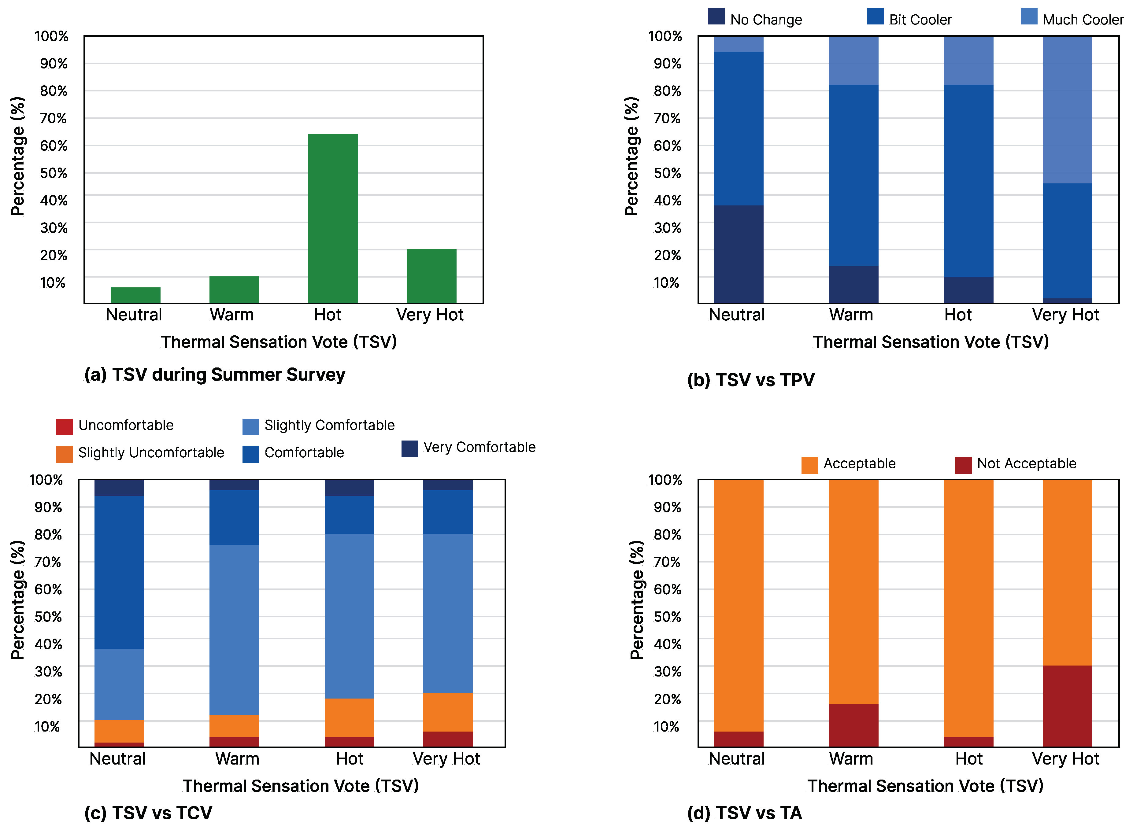
3325 responses were collected from the questionnaire survey during the summer surveys.
Figure 3a summarizes the frequency of the students’ thermal votes during summer surveys. As can be seen, TSV = 2 (Feeling Hot) category has the most votes (65%), 20% of students reported feeling very hot (TSV = 3), 10% report feeling warm (TSV = 1), and shockingly only 5% of students reported feeling neutral (TSV = 0). In contrast to the winter surveys, where about 95% of subjects’ TSV during the winter were located in the “Comfort range” (TSV = −1, 0, 1), only 16% of students voted within the comfort band during the summer t.
Figure 3b shows that with an increase in TSV from neutral (TSV = 0) to feeling very hot (TSV = 3), the percentage of students who prefer a cooler indoor environment increases from 5%, proving that students can relate the TSV with TPV. Regarding student comfort levels (TCVs), despite feeling “very hot” (TSV = 3), 21% of students voted to be comfortable (TCV = 2) and very comfortable (TCV = 3).
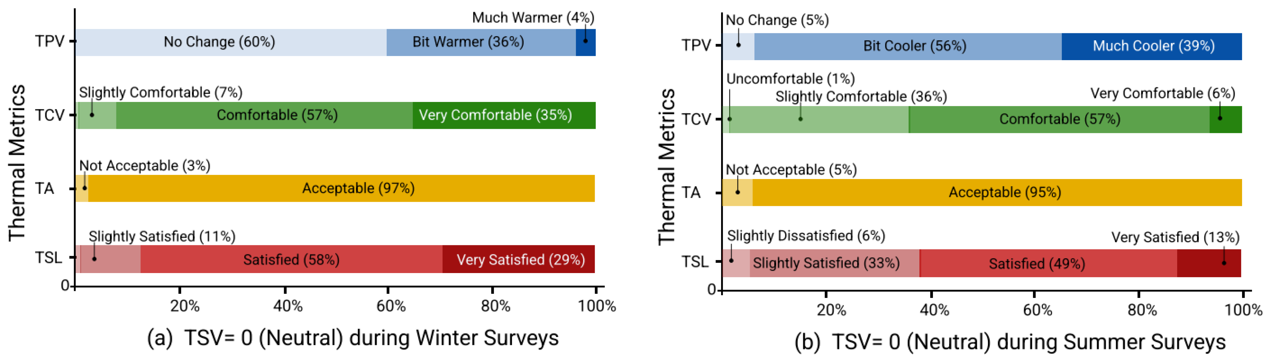
To further examine the relationship between how the students felt (sensation) and their respective thermal preference, comfort and satisfaction, the TPV, TCV, TA and TSL for TSV = 0 “neutral” is presented in
Figure 4a,b for winter and summer surveys, respectively. When TSV = 0, students have neutral sensations (neither cold nor hot), and it is observed that 60% of the students prefer no change (TPV = 0) in their indoor environment during the winter compared to 5% in the summer. A total of 93% students considered their classroom as comfortable (TCV = 2, 3) during winters in contrast to 63% during summer. Similarly, the number of students who were satisfied with their indoor environment while feeling neutral was higher during the winter (87%) than in the summer (62%).
5. System Implementation and Methodology
5.1. Correlation and Dimensionality Analysis
As a part of Exploratory Data Analysis on the dataset, both correlation and dimensional analysis were done and the following methods were used to accomplish this.
5.1.1. Correlation Techniques: Distance and Pearson
Two different techniques, namely the Pearson correlation and distance correlation method, were used to study the nature of the relationship between metrics. Distance correlation is a measure of dependence between two paired random vectors of arbitrary, not necessarily equal, dimension. Distance correlation is zero if and only if the two vectors are independent. Therefore, distance correlation measures both linear and nonlinear associations between the two vectors. In contrast, the Pearson correlation only measures the linear relationship associated with two vectors.
5.1.2. Dimensional Analysis: Principal Component Analysis
Principal Component Analysis (PCA) is a very popular dimension-reduction technique used in ML algorithms. The key idea is to map a high-dimensional point onto a lower dimension point while still being able to explain as much variance as possible. The unit vector in the lower dimension space should be the direction of a line that best fits the data while simultaneously being orthogonal to the first unit vectors. It can be shown that the principal components are eigenvectors of the data’s covariance matrix. Therefore, these are obtained by either doing a Singular Value Decomposition of the data matrix or by doing an Eigen Decomposition of the data covariance matrix.
5.2. Machine-Learning Algorithms
Support Vector Machines (SVM) and random forest (RF) classifiers are used as the primary machine-learning (ML) algorithms for the current analysis. SVM and RFs are used to predict the TC metrics to identify the minimal set of TC metrics required. A subset is considered of the most fundamental metrics which would be difficult to substitute/predict. TSV, TPV, and TCV were identified as the minimal initial subsets to predict other metrics. This decision was made as these metrics were difficult to predict from simpler metrics such as Thermal Acceptability (TA), and Satisfaction with clothing (SwC).
The logic behind selecting these two algorithms is explained as follows. Random Forests (RF) are very good when it comes to classification, they are known to converge and there is no problem with overfitting. Support Vector Machines (SVM) have been shown to learn nonlinear decision boundaries. Stratified splitting is employed for obtaining train–test split for the ML algorithms to make sure that there is a proportional representation of each class in both datasets, this splitting is carried out five times to obtain five different sets of train–test datasets derived from the original dataset. The results are then averaged out over the splits and reported.
Objectives:
- 1.
To identify the minimal set of TC metrics that can accurately predict all other metrics.
- 2.
To identify the minimal set of TC metrics that can accurately predict occupant behavior.
5.2.1. Support Vector Machines
Let
denotes the datasets considered in this workviz, ASHRAEII and the primary student dataset.
represents a vector of all the input features of a single datapoint.
is the label corresponding to the ground truth value. By the inherent nature of this problem both
comprise categorical variables. This is treated as a multiclass classification problem. Let
be the number of classes then
. Classification using Support Vector Machines is essentially binary. To make SVMs compatible with multiclass classification this work makes us of the one-vs-rest approach. Thus, if there are four classes then for each class a binary classifier (class 1 or not class 1 etc.) is used. Mathematically expressed, the aim is to solve the following optimization problem.
Here, w is the weight vector, b is the bias and is a kernel function that facilitates the learning of nonlinear classification boundaries. The method of learning nonlinear classification boundaries is to project the data point to a higher dimensional hyperplane and treat it similarly to a regular SVM problem in that dimensional space. The kernel function helps us calculate the dot product of two vectors in arbitrarily large spaces () without explicitly having to project the vectors into high-dimensional space ( or ). Results for multiple kernels viz. linear, quadratic polynomial, cubic polynomial and Radial Bias Function (RBF) have been reported further.
A regularization term is added to avoid overfitting on the training dataset, i.e., to help the model generalize better on previously unseen samples.
5.2.2. Random Forests
Random forest is an ensemble method that combines multiple decision trees and gives us the class prediction after taking a majority vote between the decision trees where each vote has equal weightage for input
x. Formally, a random forest is an ensemble of tree-structured classifiers
where
are independent and identically distributed random vectors. Decision trees are trees that follow a similar structure to the tree data structure, at every node the Gini index criteria, described below, is applied to measure the quality of the split.
where
is the number of classes
g is the Gini index (also known as Gini impurity). At every split, the one with the least Gini index is preferred. For training the random forest, the dataset is divided into subsets and individual decision tree classifiers are independently trained on them, an overlap between these subsets is allowed, and these classifiers thus predict the class independently. Finally, a majority vote is taken to generate the final class prediction, this is known as
aggregation. Random Forests are known to converge under the Strong law of large numbers.
The parameters which are used to control the nature of the random forest are the number of decision trees, whether or not the entire datasets used to generate a tree, the maximum depth of individual trees allowed, minimum samples needed to split an internal node of the decision trees.
5.2.3. Gradient Boost
Gradient Boost is a machine-learning algorithm that works on the principles of boosting. Boosting works on the principle that predictors are not made independently but sequentially, where each new model is built to rectify the errors present in the previous model.
Let us consider the algorithm proposed by Jerome H. Friedman [
30,
31]. For a given data set D =
of a known
-values, we attempt to find the best approximation for the function
, which connects inputs x to outputs y by minimizing the value of the loss function
.
here
is the weight of the
base-learner model
. Based on the number of iterations
t, new models are created iteratively.
The approximation of is obtained as
and the optimal values of the expansion coefficient
is determined by
5.2.4. Extreme Gradient Boost
Extreme Gradient Boost, also known as XGBoost is an implementation of the Gradient Boosting algorithm, proposed by Chen and Guestrin [
32]. Similar to the Gradient Boost model, it combines the predictions of multiple weaker models to create a stronger, more accurate model. It is more efficient than Gradient Boosting due to it being capable pf using the CPU’s multithreaded parallel computing to speed up the computation. The XGBoost algorithm can be described in detail as the following:
here
f represents a tree in a set of trees
F,
T represents the number of trees and
represents the
i-th eigenvector.
The objective function can be described as:
here
l is the loss function which shows the error between the predicted value and the true value. In addition,
is the regularized function that is used to prevent overfitting.
6. Correlation, Dimensionality Analysis, and Outliers
For the Correlation and Dimensionality analysis of the data collected the following metrics were considered—Thermal Satisfaction Vote (TSV), Thermal Preference Vote (TPV), Thermal Comfort Vote (TCV), Thermal Acceptability (TA), Thermal Sensation Level (TSL) and Satisfaction with Clothing. Behavioral metrics were not considered.
6.1. Correlation Analysis
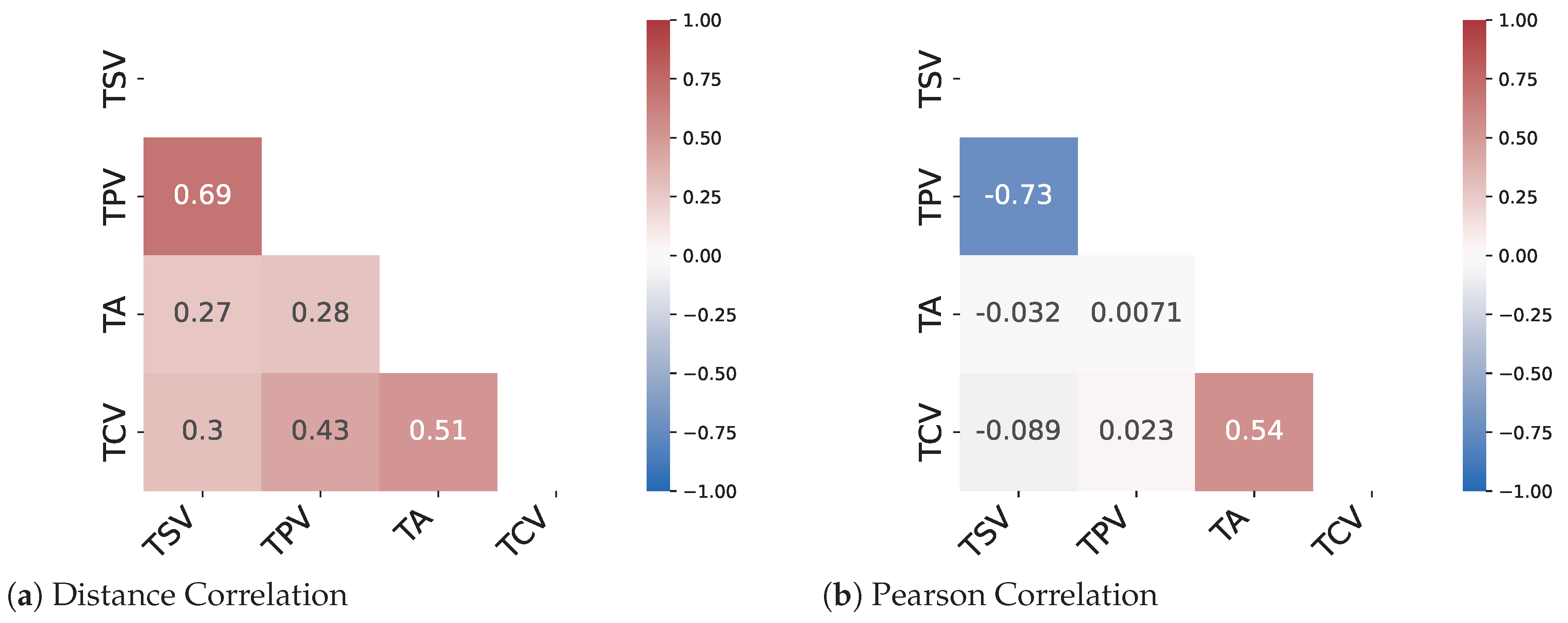
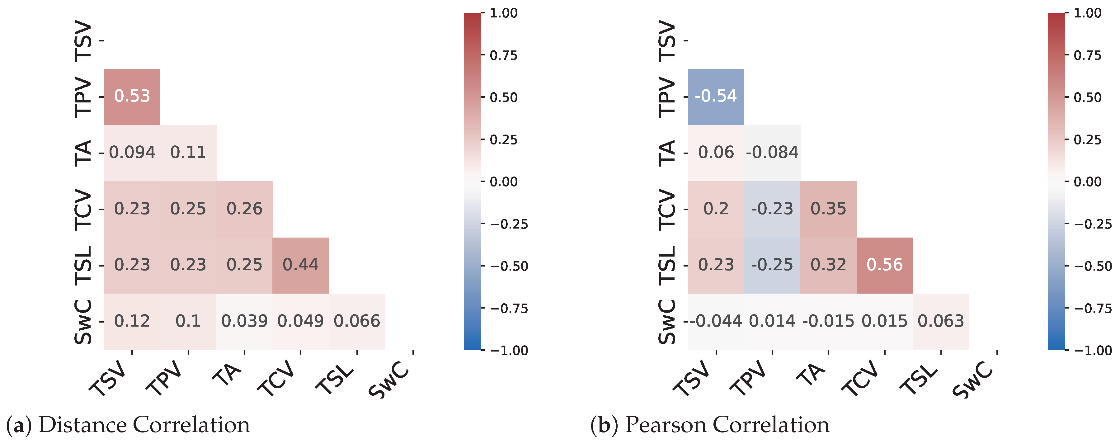
The results from the correlation analysis show that only two pairs of metrics namely (TSV-TPV) and (TCV-TSL) show a decent amount of linear correlation. The remaining metrics have a very low correlation coefficient for both the Pearson method and the distance correlation method. Therefore, a need for methods to predict nonlinear relationships between the metrics arises. As can be seen from
Figure 5 and
Figure 6 there are instances where the distance correlation is high but the Pearson correlation score is low. This can be attributed to the fact that the distance correlation score considers a nonlinear aspect of the relationship as well. Therefore, it can be assumed that for most of the metric pairs, the relationship is nonlinear in nature.
6.2. Principal Component Analysis
Principal Component Analysis or PCA is a well-known dimensionality reduction technique that also gives us insights into which axes explain the most variance in the data upon which it is applied. It is an unsupervised technique that gives us orthogonal axes as the principal components. For the data used here, PCA is applied to the metrics under consideration and it is observed that a large portion of variance can be explained by just three principal components. It is observed that for the data collected for the survey almost 86% of the variance can be explained by three principal components and almost 95% of the variance can be explained by four principal components as shown in
Table 1.
6.3. Impact of Illogical Votes
Illogical votes can be described as contradictory subjective responses by occupants in thermal comfort surveys. In a subjective thermal comfort survey, illogical votes are inevitable. These votes may be the result of a variety of factors, including when participants misinterpret the survey’s questions, flawed judgment, survey response fatigue, or some response bias. It has recently been shown that TC datasets of primary school students and children, in general, are more likely to have a higher percentage of illogical votes as compared to adults [
9,
11,
14,
28,
29]. Furthermore, the impact of illogical votes on TC prediction models has also been shown [
9,
14].
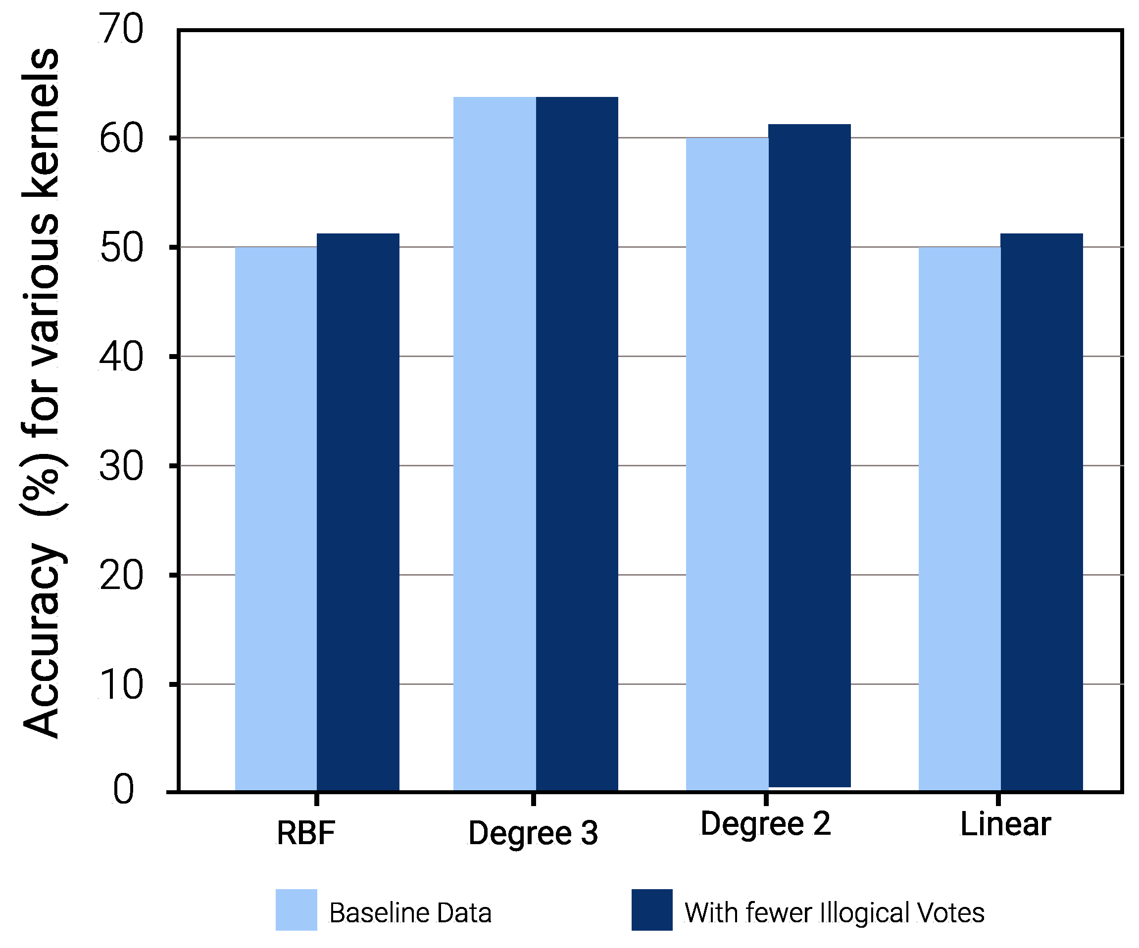
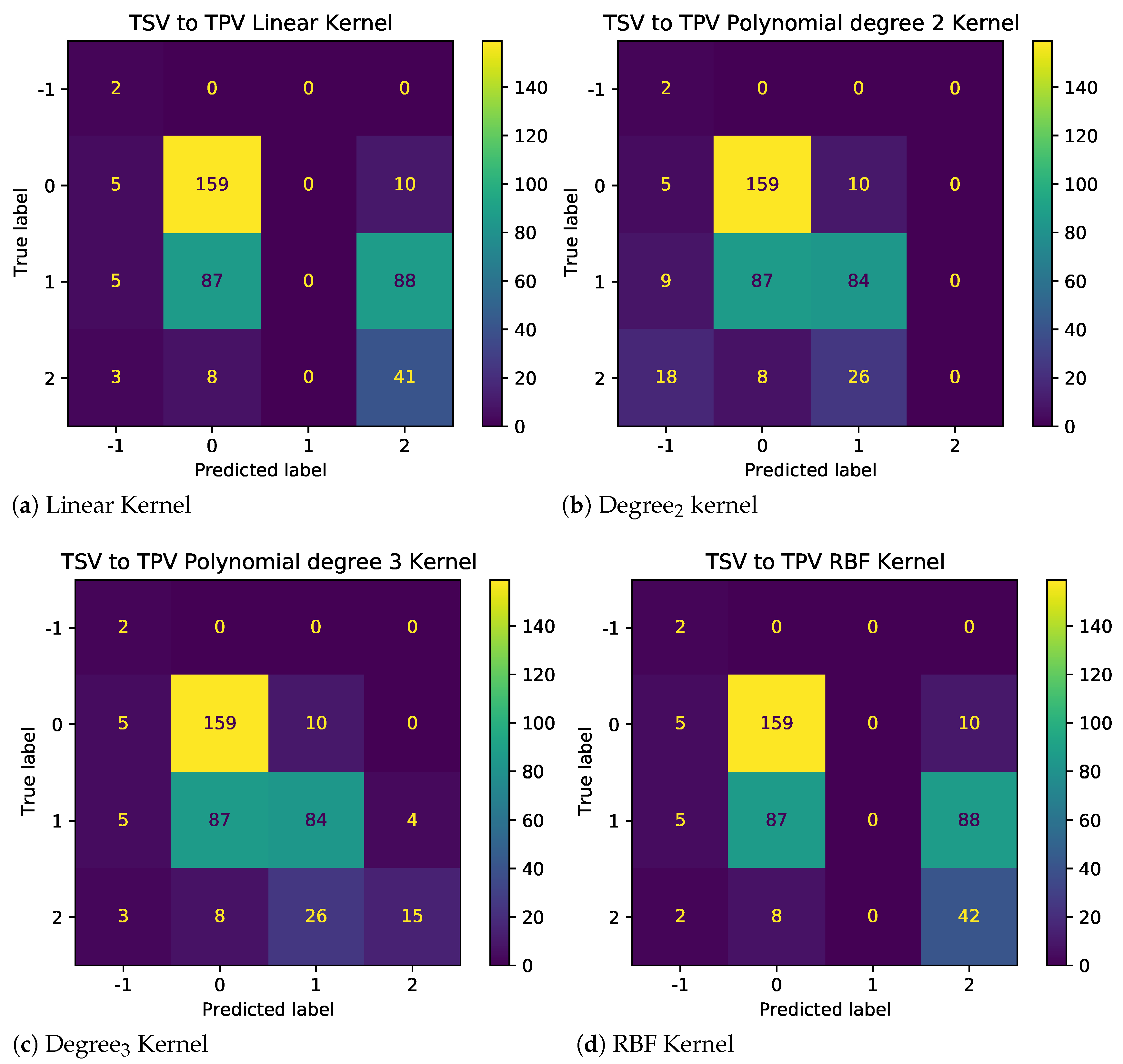
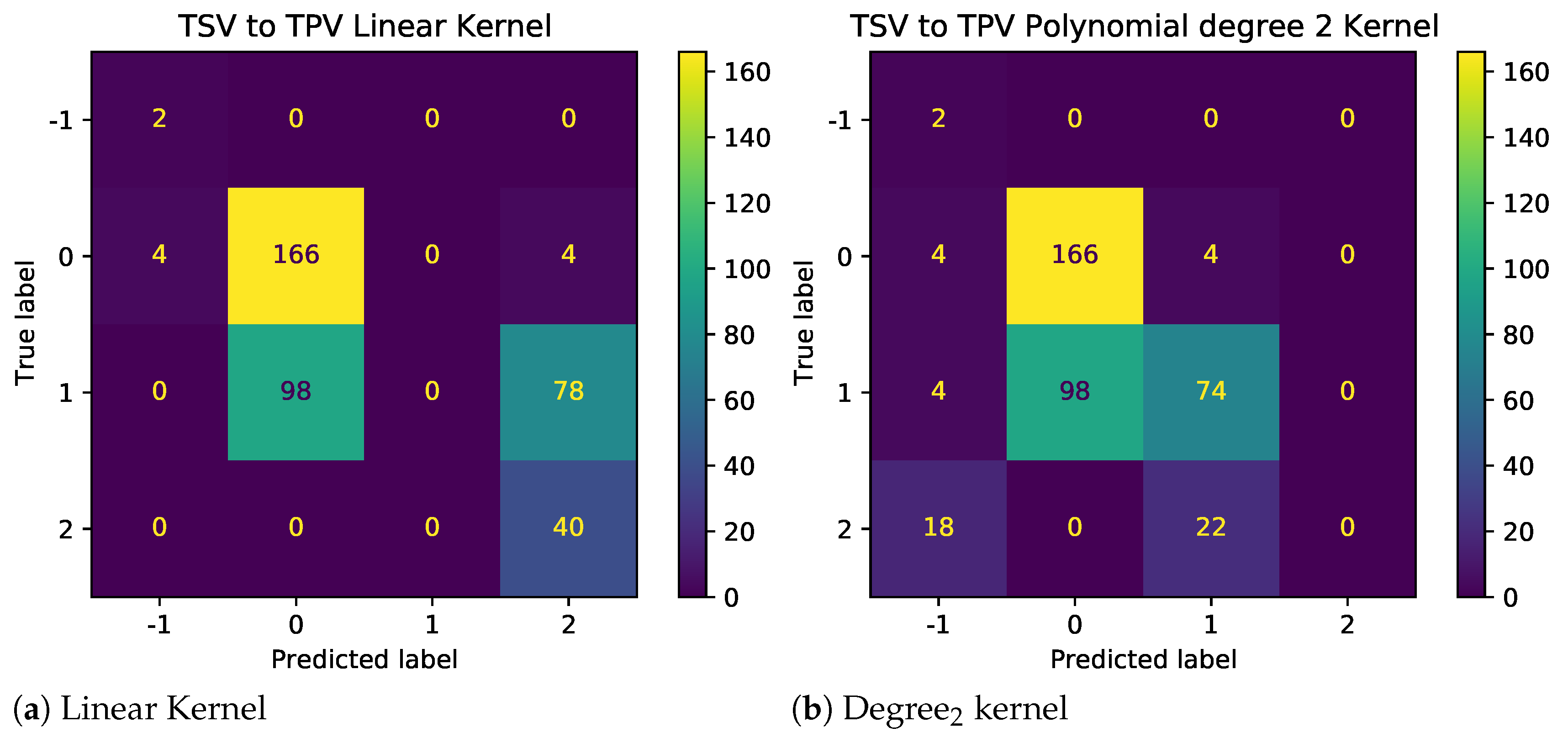
For a comprehensive evaluation, this discussion focuses on the impact of illogical votes on the prediction performance of SVM models. Winter data are considered and a primitive filter is applied to remove logically inaccurate data points. For example, it is expected that students who experience a “cool” sensation (TSV = −2) are likely to vote for a thermal preference of “warmer” or “bit warmer” (TPV = +1, +2). Therefore, in cases where TSV = −2, −3 (feeling “cold” and “cool”), if the corresponding TPV was −1 or −2 (preference of “bit cooler” and “much cooler”), that dataset was disregarded. The initial data consisting of 2039 data points was reduced to approximately 1958. The accuracies for various configurations of hyperparameters were tested and the best of those were chosen. Stratified Shuffle Sampling with five splits and train:test ratio of 80:20 was selected and the confusion matrix for the best accuracy configurations was noted down. On comparing the results for the configurations used for both consistent data (after removing outliers) and data with illogical votes, the accuracy for prediction was observed to be better after removing the noise.
The results as shown in
Figure 7 demonstrate the impact of illogical votes on the ability of different kernels to predict TPV from TSV. Two observations stand out. First, the performance of nonlinear kernels (2nd and 3rd degree) is significantly higher than those linear and radial bias unction (RBF) kernels. Thus, polynomial kernels are more suited for models used to predict other metrics using given TC metrics. Second, looking at the confusion matrices in
Figure 8 and
Figure 9, for baseline and sanitized data, respectively, there seems to be a clear impact of illogical votes on the classifier’s performance. However, it can be seen in
Figure 7 that the accuracy of nonlinear kernels does not seem to be severely impacted.
Since the determination and removal of illogical votes is subjective [
9,
14,
23], and can fundamentally alter the characteristics of the sample space, the evaluation presented ahead is performed on the baseline data. Although this makes the task more challenging, it prevents any bias in the analysis and makes the findings in this work replicable.
7. Identifying Minimal TC Metric Combination
This section analyzes all possible TC metric input combinations to identify a single TC metric or the minimal TC metric combination that can predict (a) All other TC metrics and (b) Occupant behavior, in both summer and winter seasons. The analysis is based on the F-scores, and accuracy of models involving the various input combinations. The ML algorithms considered are Gradient Boost (GBoost), Random Forest (RF), and Extreme Gradient Boost (XGBoost).
The models are trained on the primary student responses from the surveys for each season. Apart from seasonal variation, the analysis considers primary student behavior in response to classroom thermal comfort. In winter, adaptive behavior is determined by whether students modified their clothing or not. In the summer, student adaptive behavior is represented by indicators such as whether students are sweating, their fan speed preference, and satisfaction with fan speed.
Thus, the ML models in this analysis can be divided into two broad categories
- 1.
TC metrics: Here the features (input) is one or more of the TC metrics and the response variables (output) is one of the TC metrics, where TC metric ∈ {TSV, TPV, TCV, TA, TSL, SwC}.
- 2.
Occupant-Adaptive Behavior: Here the primary student occupant-adaptive behavior is the response or the label, and input is all combinations of TC metrics, where TC metric ∈ {TSV, TPV, TCV, TA, TSL, SwC}.
| Algorithm 1 Optimal Input Combination Selection |
function Best_Input_Combinations(, ) for type in ranges do Store the input_classes with the highest average_fscore in Average_res for curr_input in Average_res do Find the average_rank of the curr_input Store the average_rank to corr_avg_rank end for Display the input classes with the highest average F-score and their corresponding average rank Store the input_classes with the highest average_fscore in Rank_res for curr_input in Rank_res do Find the average_f-score of the curr_input Store the average_f-score to corr_avg_f-score end for Display the input classes with the highest average rank and their corresponding average F-score end for end function |
When building the machine-learning models, the data are split into train–test blocks using stratified K-fold shuffle with the number of splits set as 5 and a test size of 20%. Hyperparameter tuning was carried out to optimize the performance of the machine-learning models. The grid search technique was employed which searched through the range of values for each hyperparameter to identify the optimal combination that yielded the highest accuracy. For example, the maximum depth considered is 4 for GBoost, 3 for RF, and 15 for XGBoost. Similarly, the maximum number of estimators considered is 750 for GBoost, XGBoost, and RF.
The next subsection discusses Algorithm 1, which analyses ML model parameters to identify the optimalinput combination.
7.1. Optimal Input Combination Analysis
To choose the optimal input combination, ranking, F-score, and accuracy have been considered, with a preference towards ranking. The ranking of an input is determined by comparing its F-score with those of other inputs belonging to the same input class. The average F-score ranking algorithm, rank initialization algorithm, and average rank algorithm are made available in the
Appendix A and are denoted as Algorithm A1, Algorithm A2, and Algorithm A3, respectively.
Algorithm A3 determines the average rank. The input with the highest average rank across all outputs is assigned the highest rank and the ranks are referred to as average rank.
The various input classes of TC metrics include a single TC metric as a feature, combinations of two TC metrics as the feature set, combinations of three TC metrics as the feature set and so on, up to a combination of TC metrics as the feature set, TC metric being the response or the label. The optimal input combination was chosen based on their average ranking, as certain inputs can have a very high F-score for a particular response variable (output TC metric) and an average or below-average F-score for other response variables, leading to skewed results. Please note that the highest average F-score is also used when multiple inputs have the same average rank, and serves as a tie-breaker. For example, during summer, while looking for the optimal input combinations for predicting occupant behavior using XBoost Algorithm, the inputs TSV and TSL have the same average rank of 1. To choose the optimal combination, we compare the average F-score of the two inputs which are 62.5 for TSV and 63.92 for TSL. Hence we use TSL as the best optimal combination for the singular input class for the XGBoost algorithm.
Furthermore, Algorithm A2 is the rank initialization algorithm, which iterates through the input combinations for each output TC metric. It calculates the rank of a given input combination with respect to other input combinations for each output metric. Unlike the Average F-score Ranking algorithm which calculates the rank of the input combination based on the average F-score, the rank initialization algorithm calculates it only for a specific output TC metric. This algorithm iterates over all output metrics and initializes and stores the ranks of all of their respective input combinations.
Finally, Algorithm A3 computes the average rank by using the stored initialized ranks obtained from above. It iterates through the input combinations and finds the average rank of the inputs across all the output metrics. After finding the average ranks of the input combinations, it ranks them with respect to other combinations in the same input class and the final ranking is referred to as average rank.
7.2. Identifying Optimal Input Combinations
The algorithmic approach discussed above is applied to the ML model parameters (F-score, accuracy) for all input combinations. The optimal input combination for each TC metric is then identified. This section discusses the results of this process along three major themes, viz., variation across seasons, the impact of occupant behavior, and the impact of the machine-learning algorithm used.
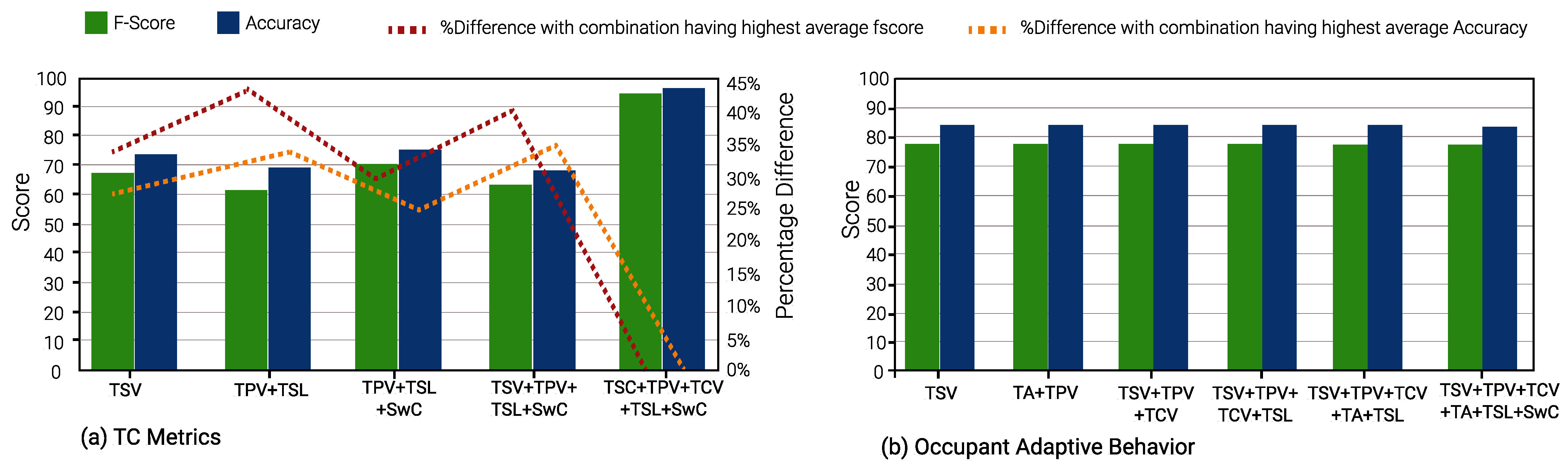
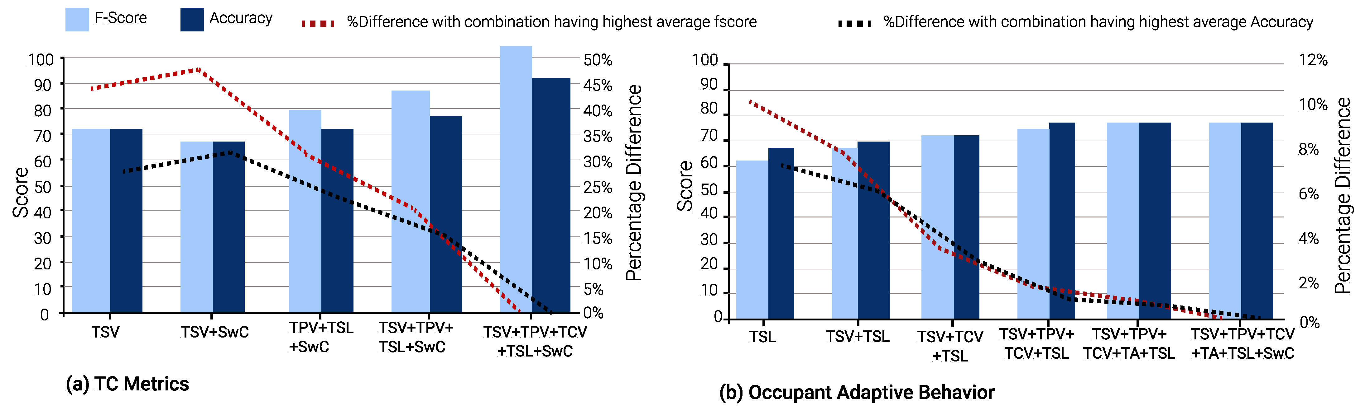
7.2.1. Impact of Seasons: Summer vs. Winter
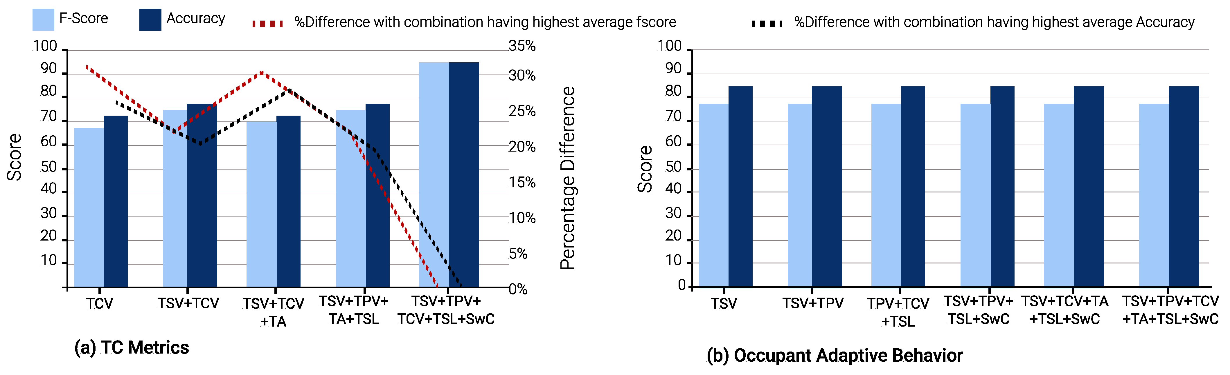
In winter, TSV is again the optimal single TC metric and is a part of 23 input combinations. TCV is the second-best TC metric, appearing in 21 input combinations. This is evident from
Figure 10,
Figure 11 and
Figure 12.
Figure 10 and
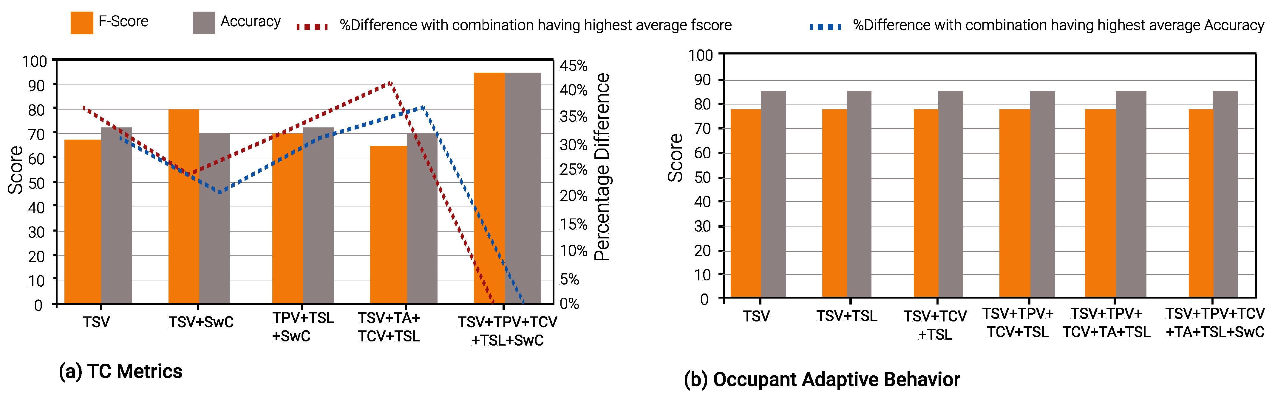
Figure 13 shows the results of Gradient Boost Algorithm for Winter and summer surveys, respectively. In summer, TSV is the single most suitable metric in various input combinations to predict all other TC metrics, viz., TPV, TCV, TSL, TA, and SwC. It appears in 28 input combinations across all TC prediction models considered. TSL is the second most suitable input metric, occurring 26 times in input combinations across all ML models. This can be discerned from
Figure 13,
Figure 14 and
Figure 15.
It can be seen in
Figure 13b,
Figure 14b and
Figure 15b that the percentage of difference in accuracy between the highest thermal comfort metric and others is almost negligible for Occupant Behavior prediction models. This can be explained due to the skewed data imbalance in the number of students who modified their clothing (adaptive behavior) during winter surveys. Only 12% of the students removed a layer of clothing item, 4% wore extra clothing and the remaining 84% did not modify their clothing.
In terms of the average F-scores of the ML models for summer and winter, the average value (76.11%) in winter is greater than those in the summer (72.12%) for corresponding models. The same holds for model accuracy as well, with 76.12% as the average accuracy for summer TC prediction models and 81.33% for winter models.
An interesting observation can be seen in
Figure 10b,
Figure 11b and
Figure 12b. During the winter, the percentage difference between F-score and accuracy for the “Occupant Behavior” prediction models is less than 1%, when compared to the input combination with the highest F-score and accuracy. Furthermore, most F-scores hover around 77% and model accuracies around 84%. In contrast, in the summer, the difference in the two parameters for Occupant Behavior models can be up to 11% and 7% in comparison to the input combination with the highest F-score and accuracy.
Thus, for prediction models for occupant behavior, optimal minimal input combinations are quite close to the input combinations with the best model performance. This is particularly useful, as the adaptive behavior of occupants can be predicted with a minimal TC metric input without the use of a larger feature set such as classroom environment features (indoor temperature, humidity, air velocity, etc.), external features (outdoor temperature, daily average temperature, average rainfall and humidity, etc.), and miscellaneous features (age, gender, metabolic rate, etc.).
7.2.2. Impact of Occupant Behavior
The performance of ML models that predict TC metrics as an output differs from those that predict occupant behavior or action. In summer, the average F-scores of models predicting TC metrics are usually higher than the average F-scores of models predicting occupant behavior. This can be observed in
Figure 13,
Figure 14 and
Figure 15. However, the same is not true for winter. Here, TC models predicting occupant-adaptive behavior have a higher average F-score when compared to those predicting other TC metrics. This difference in results between seasons can be attributed to the fact that in the summer, the occupant action involves labels such as fan speed preference, sweating, and fan satisfaction while in winter, occupant action is just limited to modified clothing (MC).
For summer TC metric prediction models, it can be observed that models with TSV and (TSV, TPV, TCV, TSL, and SwC) as features provide the highest average F-score. Furthermore, input combinations (TSV, SwC) and (TSV, TPV, TSL, SwC) demonstrate the highest F-score for both RF and XGBoost algorithms. In the case of inputs predicting occupant behavior such as modified clothing in winter and sweating in summer, feature combinations (TSV, TPV, TCV, TSL), (TSV, TPV, TCV, TA, TSL) and (TSV, TPV, TCV, TA, TSL, SwC) lead to the highest average F-scores for all ML algorithms. Furthermore, TSV as the only feature leads to the highest F-score for GBoost and RF algorithms while the input combination (TSV, TCV, TSL) leads to the highest F-score for RF and XGBoost algorithms.
During winter, it is evident that for TC metric prediction models, the best input combination in terms of F-score is (TSV, TPV, TCV, TSL, and SwC) across all ML algorithms. However, the input class consisting of five features is not desirable as responses for all 5 TC metrics need to be gathered from the occupants and only one TC metric, such as TA in this case, remains to be predicted. Furthermore, TCV seems to be the single optimal TC metric to predict all other metrics through RF and XGBoost algorithms. Furthermore, the input (TPV, TA, TSL, SwC) provides the highest F-score for the GBoost and RF algorithms. For models predicting adaptive behavior, TSV is the only feature that offers the highest F-score irrespective of the ML algorithms.
A unique observation concerning Occupant Behavior prediction models in winter is that the average F-score and accuracy across all input combinations is approximately 77% and 84%, respectively. The difference, when compared to the best-performing input combination, is less than 1%. Furthermore, when adaptive behavior model performance for summer and winter seasons is analyzed together, the percentage difference, compared to the best-performing input combination, is ≈11%. However, for models that predict other TC metrics, the percentage difference can go up to 40% for F-score, vis-a-vis the best-performing input combination.
This finding indicates that predicting other TC metrics from a single TC metric or a minimal set of TC metrics is a difficult task. However, occupant-adaptive behavior or action as an indicator of a thermal comfort environment is far easier to predict. This is because while subjective responses may have inconsistencies, especially when it comes to children, the adaptive action is more objective and less ambiguous.
7.2.3. Impact of the Machine-Learning Algorithm
It can be observed that Gradient Boost (GBoost) consistently offers the lowest averaged F-score and the lowest average accuracy among the three ML algorithms considered in this work. In contrast, Extreme Gradient Boost (XGBoost) has the highest averaged F-score and accuracy, and the Random Forest (RF) algorithm is a close second. Therefore, the choice of ML algorithm also seems to have an impact on the performance of models that predict Occupant Behavior or other TC metrics.
Let us consider the objective of identifying the minimal input combination which is most suitable to predict all other TC metrics, in winter. The Optimal Input Combination Selection algorithm yields TSV as the optimal single feature for GBoost and RF, while TCV is the same for XGBoost. Furthermore, the optimal two-feature input combinations also differ, i.e., (TPV, TSL) by GBoost, (TSV, SwC) by RF, and (TSV, TCV) by XGBoost.
Thus, both the model output and model performance vary depending on the choice of ML algorithm.
7.3. Optimal TC Metrics: Is TSV Enough?
TSV, TPV, TCV, TA, and TSL are the most commonly used thermal comfort indices, and the correlation between each parameter is undeniable [
23]. However, the majority of TC research considers TSV to be the primary indicator of occupant thermal comfort [
20,
23,
33]. The findings of this study also present similar results, as demonstrated by
Figure 10 to
Figure 15. Results indicate that TSV has a significant potential to predict thermal comfort and occupant-adaptive behavior as a single TC metric.
The first objective of this study was to determine the most important single TC metric. There are 12 broad scenarios in our evaluation comprising three ML algorithms (GBoost, RF, and XGBoost), two seasons (summer and winter), and type of prediction models (TC metric and Occupant Behavior). We consider these 12 scenarios to analyze the most important TC metric along two factors.
First, what is the TC metric that offers the highest prediction performance (F-score and accuracy) when used as the only feature/input in the model? TSV is the most frequent TC metric, as it offers the best performance in 8/12 scenarios, followed by TSL (2 scenarios), and TCV (2 scenarios). It is interesting to note that thermal preference (TPV) is not the optimal TC metric in even one scenario. Thus, it is suitable to consider TSV as the sole TC metric and determine/predict other TC metrics through it.
Second, when considering input combinations of multiple TC metrics, leading to inputs of multiple features, which one is the most common TC metric? In two-feature inputs, TSV is a part of the feature set in seven scenarios, TSL in five scenarios, TPV in four scenarios, SwC in four scenarios, TCV in three scenarios, and TA in one scenario. Further combinations of TSV with SwC, TSV, and TPV are the optimal combinations in 6 out of 12 scenarios. In three-feature inputs, both TSV and TSL are the most common features, each appearing in eight input feature sets, followed by TCV in 7, and TPV and SwC in six scenarios. In four-feature combinations, TSL is a feature in all 12 scenarios, followed by TSV and TPV, which appear 10 times each, and finally SwC and TCV six times each.
Therefore, it can be stated that, as a single metric, TSV is the most important, and the ideal starting point in subjective questionnaires. As the number of TC metrics increases, TSL also gains importance. TPV and SwC seem to be next in priority followed by TCV. Interestingly, satisfaction with clothing is found to be as important as thermal preference, as it is rarely considered in existing studies.
8. Conclusions and Way Forward
This study aimed to determine a minimal set of thermal comfort (TC) metrics that could accurately predict all other metrics and identify the optimal combination of input metrics for predicting occupant-adaptive behavior. To do so, it proposed an innovative Optimal Input Combination Selection algorithm based on input combination ranking.
Furthermore, the study demonstrated that ML algorithms can use a minimal subset of TC metrics to predict other TC metrics with high accuracy. For example, the Extreme Gradient Boost Algorithm demonstrated an average accuracy of 79% and outperformed other ML algorithms.
It was observed that TSV is the most significant indicator as a single metric for thermal comfort, followed by TSL. Furthermore, SwC was shown to be just as significant as TPV, which is an important finding as thermal comfort studies rarely make use of clothing satisfaction as a measure of thermal comfort.
Additionally, the study has demonstrated that the input combinations (usually comprising five features) with the best model performance are close to the optimal minimum input combinations identified by the proposed algorithm when predicting occupant-adaptive behavior. The difference in Occupant Behavior prediction could be as low as 1% in winter. This is significant considering the adaptive behavior of students may be predicted using a relatively small amount of TC metrics. This finding also relaxes the requirement for a comprehensive feature set comprising indoor, environmental, physiological, and social features.
Results indicate that it is challenging to reliably predict other TC metrics from a single TC metric or a minimal subset of TC metrics. By contrast, occupant-adaptive behavior as an indicator of thermal comfort can be predicted more reliably. A plausible reason for this is that adaptive behavior is more objective and unambiguous as compared to subjective responses, which can be inconsistent, especially when participants are children or primary students.
Finally, both model output and model performance vary depending on the choice of ML algorithm. The seasonal impact on optimal TC metric or minimal TC metric combination was also shown.
Author Contributions
Conceptualization, B.L. and S.M.K.; methodology, B.L., S.M.K. and A.H.; software, A.B., V., A.R. and K.D.; formal analysis, B.L. and S.M.K.; investigation, B.L.; resources, A.H.; data curation, B.L.; writing—original draft, B.L., A.B., A.R. and S.M.K.; writing—review & editing, B.L. and S.M.K.; visualization, B.L.; supervision, S.M.K. and A.H.; project administration, S.M.K. and A.H.; funding acquisition, A.H. All authors have read and agreed to the published version of the manuscript.
Funding
This work was supported by the Ministry of Education, Culture, Sports, Science, and Technology (MEXT) KAKENHI Grant Number JP22H01652.
Conflicts of Interest
The authors declare no conflict of interest.
Appendix A
In order to choose the input combinations with can best predict our desired outputs, we first use the “Average F-score Ranking” (A1) to calculate the average the average F-score of the input, and it’s respective ranking to other input combinations of the same input class. After that, we use “Rank Initialization” algorithm (A2) to determine the rank of the input with respect to other inputs of the same input class for the selected output class. Following this, we use “Average Rank Ranking” algorithm (A3) to calculate the average rank of the input with respect to all the output’s across the board and then to find the ranking of the input with respect to other inputs of the same input class.
| Algorithm A1 Average F-score Ranking |
function Average_Fscore_Ranking Initialize Average_matrix as a list for type in ranges do ▹ “ranges” is the input combinations Initialize start_range with the beginning of the selected range Initialize end_range with the end of the selected range Initialize temp_avg_array as a list Initialize Average_dict as a dictionary for current in input_classes_location[start_range:end_range] do ▹ “current” is the input Calculate the average of the chosen input and store it in “res”. Store “res” in temp_avg_array. end for Calculate the rank of input classes from temp_avg_array Store the ranks in the result for chosen_rank in result do Store the chosen_rank to Average_dict with its corresponding input end for Store average_dict to an average_matrix which corresponds to its combination type. end for end function
|
| Algorithm A2 Rank Initialization |
function Rank Initialization for curr_output in output_classes_location do ▹ curr_output is the chosen output for type in ranges do ▹ “ranges” is the input combinations Initialize start_range with the beginning of the selected range Initialize end_range with the end of the selected range Initialize temp_avg_array as a list for current_input in input_classes_location[start_range:end_range] do Collect the F-score of the current_input for the chosen output Store the F-score to temp_rank_array end for Calculate the rank of input classes from temp_avg_array Store the ranks in the result for chosen_rank in result do Store the chosen_rank to Average_dict with its corresponding input end for end for Store Average_dict to an Average_Rank_matrix which corresponds to its output end for end function
|
| Algorithm A3 Average Rank Ranking |
function average ranking() Initialize Rank_matrix as a list for type in ranges do Initialize start_range with the beginning of the selected range Initialize end_range with the end of the selected range Initializes rank_averages as a list Initializes Rank_dict as a dictionary for current_input in input_classes_location[start_range:end_range] do Calculate the average rank of the current_input Store “res” in rank_averages. end for Calculate the rank of the input classes from rank_averages for chosen_rank in result do Store the chosen_rank to Average_dict with its corresponding input end for Store Average_dict to a Rank_matrix which corresponds to its combination type end for end function
|
References
- Philomena, M.B. The Indoor Environment Handbook: How to Make Buildings Healthy and Comfortable; Earthscan: London, UK, 2009. [Google Scholar]
- Wyon, D.; Andersen, I.; Sundell, J.; Clements-Croome, D. The effects of moderate heat stress on mental performance. Scand. J. Work Environ. Health 1979, 5, 352–361. [Google Scholar] [CrossRef] [PubMed] [Green Version]
- Fanger, P.O. Thermal comfort analysis and applications in environmental engineering. In Thermal Comfort. Analysis and Applications in Environmental Engineering; Danish Technical Press: København, Denmark, 1970. [Google Scholar]
- De Dear, R.; Brager, G.S. Developing an Adaptive Model of Thermal Comfort and Preference; UC Berkeley: Berkeley, CA, USA, 1998. [Google Scholar]
- Gan, V.J.; Luo, H.; Tan, Y.; Deng, M.; Kwok, H. BIM and data-driven predictive analysis of optimum thermal comfort for indoor environment. Sensors 2021, 21, 4401. [Google Scholar] [CrossRef] [PubMed]
- Tahmasebinia, F.; Jiang, R.; Sepasgozar, S.; Wei, J.; Ding, Y.; Ma, H. Implementation of BIM energy analysis and monte carlo simulation for estimating building energy performance based on regression approach: A case study. Buildings 2022, 12, 449. [Google Scholar] [CrossRef]
- Arakawa Martins, L.; Soebarto, V.; Williamson, T. A systematic review of personal thermal comfort models. Build. Environ. 2022, 207, 108502. [Google Scholar] [CrossRef]
- Qavidel Fard, Z.; Zomorodian, Z.S.; Korsavi, S.S. Application of machine learning in thermal comfort studies: A review of methods, performance and challenges. Energy Build. 2022, 256, 111771. [Google Scholar] [CrossRef]
- Lala, B.; Rizk, H.; Kala, S.M.; Hagishima, A. Multi-task learning for concurrent prediction of thermal comfort, sensation and preference in winters. Buildings 2022, 12, 750. [Google Scholar] [CrossRef]
- Fuchs, M. Children and adolescents as respondents. Experiments on question order, response order, scale effects and the effect of numeric values associated with response options. J. Off. Stat. 2005, 21, 701. [Google Scholar]
- Lala, B.; Kala, S.M.; Rastogi, A.; Dahiya, K.; Hagishima, A. Are You Comfortable Now: Deep Learning the Temporal Variation in Thermal Comfort in Winters. In Proceedings of the 2022 IEEE International Conference on Systems, Man, and Cybernetics (SMC), IEEE, Prague, Czech Republic, 9–12 October 2022; pp. 1848–1855. [Google Scholar]
- Lala, B. Analysis of thermal comfort study in india. In Proceedings of the International Conference on Civil, Architecture, Environment andWaste Management (CAEWM-17), Singapore, 29–30 March 2017. [Google Scholar]
- Qi, J.; Wang, J.; Zhai, W.; Wang, J.; Jin, Z. Are There Differences in Thermal Comfort Perception of Children in Comparison to Their Caregivers’ Judgments? A Study on the Playgrounds of Parks in China’s Hot Summer and Cold Winter Region. Sustainability 2022, 14, 10926. [Google Scholar] [CrossRef]
- Lala, B.; Hagishima, A. A Review of Thermal Comfort in Primary Schools and Future Challenges in Machine Learning Based Prediction for Children. Buildings 2022, 12, 2007. [Google Scholar] [CrossRef]
- Bradbury-Jones, C.; Taylor, J. Engaging with children as co-researchers: Challenges, counter-challenges and solutions. Int. J. Soc. Res. Methodol. 2015, 18, 161–173. [Google Scholar] [CrossRef] [Green Version]
- Borgers, N.; De Leeuw, E.; Hox, J. Children as respondents in survey research: Cognitive development and response quality 1. Bull. Sociol. Methodol. 2000, 66, 60–75. [Google Scholar] [CrossRef] [Green Version]
- De Leeuw, E.D. Improving Data Quality when Surveying Children and Adolescents: Cognitive and Social Development and its Role in Questionnaire Construction and Pretesting. 2011. Available online: https://www.aka.fi/globalassets/tietysti1.fi/awanhat/documents/tiedostot/lapset/presentations-of-the-annual-seminar-10-12-may-2011/surveying-children-and-adolescents_de-leeuw.pdf (accessed on 18 February 2023).
- Brower, C.K. Too Long and Too Boring: The Effects of Survey Length and Interest on Careless Responding. Ph.D. Thesis, Wright State University, Dayton, OH, USA, 2018. [Google Scholar]
- Leung, W.C. How to design a questionnaire. BMJ 2001, 322, 0106187. [Google Scholar] [CrossRef] [Green Version]
- Schweiker, M.; Fuchs, X.; Becker, S.; Shukuya, M.; Dovjak, M.; Hawighorst, M.; Kolarik, J. Challenging the assumptions for thermal sensation scales. Build. Res. Inf. 2017, 45, 572–589. [Google Scholar] [CrossRef] [Green Version]
- Kim, J.; Schiavon, S.; Brager, G. Personal comfort models—A new paradigm in thermal comfort for occupant-centric environmental control. Build. Environ. 2018, 132, 114–124. [Google Scholar] [CrossRef] [Green Version]
- Ma, N.; Chen, L.; Hu, J.; Perdikaris, P.; Braham, W.W. Adaptive behavior and different thermal experiences of real people: A Bayesian neural network approach to thermal preference prediction and classification. Build. Environ. 2021, 198, 107875. [Google Scholar] [CrossRef]
- Wang, Z.; Wang, J.; He, Y.; Liu, Y.; Lin, B.; Hong, T. Dimension analysis of subjective thermal comfort metrics based on ASHRAE Global Thermal Comfort Database using machine learning. J. Build. Eng. 2020, 29, 101120. [Google Scholar] [CrossRef] [Green Version]
- Ansi, A.; Ashrae, M. ANSI/ASHRAE Standard 55; Thermal Environmental Conditions for Human Occupancy. ASHRAE: Atlanta, GA, USA, 2004. [Google Scholar]
- CEN E. 15251; Indoor Environmental Input Parameters for Design and Assessment of Energy Performance of Buildings Addressing Indoor Air Quality, Thermal Environment, Lighting and Acoustics. European Committee for Standardization: Brussels, Belgium, 2007.
- Xie, J.; Li, H.; Li, C.; Zhang, J.; Luo, M. Review on occupant-centric thermal comfort sensing, predicting, and controlling. Energy Build. 2020, 226, 110392. [Google Scholar] [CrossRef]
- Ngarambe, J.; Yun, G.Y.; Santamouris, M. The use of artificial intelligence (AI) methods in the prediction of thermal comfort in buildings: Energy implications of AI-based thermal comfort controls. Energy Build. 2020, 211, 109807. [Google Scholar] [CrossRef]
- Lala, B.; Kala, S.M.; Rastogi, A.; Dahiya, K.; Yamaguchi, H.; Hagishima, A. Building matters: Spatial variability in machine learning based thermal comfort prediction in winters. In Proceedings of the 2022 IEEE International Conference on Smart Computing (SMARTCOMP), IEEE, Espoo, Finland, 20–24 June 2022; pp. 342–348. [Google Scholar]
- Lala, B.; Murtyas, S.; Hagishima, A. Indoor thermal comfort and adaptive thermal behaviors of students in primary schools located in the humid subtropical climate of india. Sustainability 2022, 14, 7072. [Google Scholar] [CrossRef]
- Friedman, J.H. Stochastic gradient boosting. Comput. Stat. Data Anal. 2002, 38, 367–378. [Google Scholar] [CrossRef]
- Natekin, A.; Knoll, A. Gradient boosting machines, a tutorial. Front. Neurorobotics 2013, 7, 21. [Google Scholar] [CrossRef] [PubMed] [Green Version]
- Chen, T.; Guestrin, C. Xgboost: A scalable tree boosting system. In Proceedings of the 22nd ACM SIGKDD International Conference on Knowledge Discovery and Data Mining, San Francisco, CA, USA, 13–17 August 2016; pp. 785–794. [Google Scholar]
- Shahzad, S.; Brennan, J.; Theodossopoulos, D.; Calautit, J.K.; Hughes, B.R. Does a neutral thermal sensation determine thermal comfort? Build. Serv. Eng. Res. Technol. 2018, 39, 183–195. [Google Scholar] [CrossRef]
| Disclaimer/Publisher’s Note: The statements, opinions and data contained in all publications are solely those of the individual author(s) and contributor(s) and not of MDPI and/or the editor(s). MDPI and/or the editor(s) disclaim responsibility for any injury to people or property resulting from any ideas, methods, instructions or products referred to in the content. |
© 2023 by the authors. Licensee MDPI, Basel, Switzerland. This article is an open access article distributed under the terms and conditions of the Creative Commons Attribution (CC BY) license (https://creativecommons.org/licenses/by/4.0/).


 ,
, 


