Passive Intelligent Kinetic External Dynamic Shade Design for Improving Indoor Comfort and Minimizing Energy Consumption

Abstract

In humid subtropical climates with a green environment, windows are the most dominant envelope elements affecting indoor visual and thermal comfort and visual connection to the outdoors. This research aims to optimize a dynamic external shading system for north-facing windows in Sydney, Australia, which acts automatically in eight predefined scenarios in response to indoor comfort conditions. The method of investigation was simulating a multi-objective optimization approach using Non-dominated Sorting Particle Swarm Optimization (NSPSO) to assess visual and thermal comfort along with energy usage and view of the outside. A combination of human and sensor assessments were applied to validate the simulations. A set of sensors and High Quality (HQ) cameras fed the system input to operate the shade. Simulations and field measurements demonstrated that optimized shading scenarios brought average yearly reductions of 71.43%, 72.52%, and 1.78% in Annual Solar Exposure, Spatial Daylight Glare, and LEED Quality View, respectively, without sacrificing Daylight Autonomy. Moreover, yearly improvements of 71.77% in cooling demand were achieved. The downside of the shading system was an increase of 0.80% in heating load and 23.76% in lighting electricity, which could be a trade-off for improved comfort and energy savings. This study investigated the effect of dynamic external shade on visual and thermal comfort together with energy usage and view, which has not been investigated for southern-hemisphere dwellings. A camera-sensor-fed mechanism operated the external shade automatically, providing indoor comfort without manual operation.

1. Introduction

A sense of growing apprehension in the matter of comfort has aroused people’s concern about their living conditions, such as acoustic, thermal, and luminous comfort [1]. According to the National Human Activity Pattern Survey (NHAPS), an average of 87% of people’s time is spent in enclosed buildings [2]. Sunlight is a multisensory topic that could affect the quality of dynamic luminous, health, thermal, and visual comfort [3,4,5,6]. In addition to sunlight’s substantial role in producing natural vitamins and hormones [7], a dynamic relationship exists between daylight and indoor human activities and behavioral models [3,5,8,9,10].

As indicated in the literature, looking through windows and “visual connections with the landscape and life on the ground plane” [11] are essential for efficient daylight design [7]. Accordingly, researchers have recently shown increased interest in climate-adaptive building envelopes as a “promising alternative for higher levels of sustainability in the built environment” [12].

Dwellings account for 25% of buildings’ energy consumption, 40% of total energy consumption, and 36% of CO₂ emissions [13]. According to the International Energy Agency (IEA), from 1990 to 2020, Australia experienced a rise of 73.3% and 44.7% in final electricity consumption and total CO₂ emissions, respectively. Regarding daylight admission and energy consumption, artificial lighting accounts for 19% of worldwide electrical consumption [13] and the highest primary energy load (over 30% of the total energy consumption) in buildings, mainly during the daytime. The cooling load is the most rapidly increasing primary energy load in buildings [7,11]. Deflecting sunlight into the indoor environment can reduce electric lighting by at least 50% [7]. An effective method of daylight admission controlled by technologies or systems could maintain the lighting energy and cooling loads minimum [7,13,14,15,16] and even help decrease heating loads. Therefore, using sunlight for natural illumination without overheating could be a significant alternative energy source in the building sector to improve energy savings and sustainability [6]. Moreover, a proper automatic control strategy would promote selective daylight admission into an indoor environment [16].

In response to the dynamic appeal of levelling sunlight delivery [7], shading systems, along with the façade size and glazing, define energy, and visual performances [17,18] would bring some advantages such as absorbing more heat in the heating season, securing shading, and bringing passive comfort in the cooling season. An efficient shading system requires incorporating the Sun’s elevation angles in order to control seasonal thermal radiation and light transmission properly [7]. Building envelope optimization maximizes natural light and visual contact with the outdoors while minimizing energy consumption. In other words, the fundamental aim of optimizing building envelopes is to maintain the balance between daylight harvesting (as a free and natural energy resource) and to maximize visual contact with the outside while minimizing visual discomfort and building energy consumption [16]. In this regard, daylight-management systems (as a part of envelope optimization) are the main focus in achieving buildings’ energy saving and reducing the carbon footprint [7,19]. Thus, sunlight-control devices in residential buildings enhance thermal and visual comfort while taking advantage of solar gains to decrease heating loads [20] and can be used as a supplement or substitute for artificial illumination, although it can negatively impact cooling loads. Many daylight-management systems focus on minimizing the negative impacts while ignoring their positive effects on indoor comfort that usually result in counterpart artificial lighting [13].

Smart glasses such as electrochromic glasses—as a component of the Responsive Building Envelope (RBE)—could save energy and enhance indoor visual and thermal comfort, with a profound impact on the reduction of cooling demand [21].

To design a penetration feature, several contradictory criteria should be taken into consideration: daylight illuminance and view against glare [16,22,23,24]; visual versus thermal comfort [1,18,24,25,26,27]; privacy versus view [16,24]; solar gain versus overheating [16]; and natural illumination versus electric lighting [7].

Several attempts have been made to assess the effect of shading systems, both fixed and movable, on indoor comfort. However, the majority of research has focused on office spaces (as shown in Figure 1). Furthermore, previous studies have mainly concentrated on visual comfort metrics or energy consumption (as also shown in Figure 1), and there is a lack of comprehensive analysis that takes into account both visual and thermal comfort along with the corresponding energy consumption. Additionally, the impact of shading systems on blocking views to the outside has been overlooked. While some studies have attempted to optimize the surface of internal shading systems, such as Venetian blinds, there is limited research on optimizing the surface of external shading elements due to the challenges of moving them.

In view of all that has been mentioned so far, the motivation of the present study is to provide an understanding of the proper predefined patterns to automatically move an external shading element that acts as a light shelf and shade on the most prominent window in residential buildings in Sydney, Australia. The aim of the study was to promote home-office visual comfort and energy performance to achieve a homeostatic balance. These findings have important implications for removing the occupants’ continuous readjustment of shading elements.

2. Literature Review

The majority of research on window and shading systems has been focused on minimizing energy consumption, hence disregarding indoor visual comfort [28]. Gago et al. (2015) proved that daylight admission control methods alleviate glare and maximize indoor illuminance [13]. Köster (2020) explained that in a mixed climate region such as Sydney, maintaining the daylight needs to be supplemented by dynamic shading to secure optimal energy management on a seasonal or time-of-day basis [7].

De Michele et al. (2018) simulated a multi-objective control strategy and achieved 10% cooling energy saving [29]. Using multi-objective optimization, Valitabar et al. (2021) studied adaptive façades to find a balance between visual comfort and operational energy while allowing visual contact with the outside. They demonstrated that using an optimum external multi-layer dynamic vertical shading in Tehran, Iran improves the performance by up to 10% [22]. Im et al. (2019) studied the angle of dynamic façade system effect on solar heat gain, daylighting, and user satisfaction to find an optimum angle of dynamic façade system for an office in Charlotte, NC, USA. They developed a dynamic control scheme by a min–max normalization technique that resulted in a 10% improvement in daylight performance [30]. Assessing energy consumption and cooling load, De Luca et al. (2018) carried out a detailed comparison between static and moveable systems’ performance for an office in Tallinn, Estonia [31]. They showed that by using solar shading on office buildings with large windows (WWR = 55–70%), the cooling energy demand decreases by up to ten times. Konstantzos et al. (2015) studied view purity through window shades for offices in West Lafayette, IN, USA, where they quantified view clarity based on fabric type, sky conditions, and viewing distance [32].

According to Abboushi et al. (2020), the literature on sunlight exposure does not address the possible effects of sunlight patterns on indoor visual comfort [4], while the luminous comfort level in residential buildings is strongly influenced by satisfaction with daylighting [1]. According to Mardaljevic, all the daylight/sunlight planning methods up to 2021 fail to estimate “performance at the outset” [5].

Carmody and Haglund (2006) categorized external shading devices as horizontal on the top edge of a window (overhang) and vertical shades on the side edges (fin) [33]. The immovable shading elements restrain daylight admission during overcast sky conditions [31]. De Luca et al. (2018) affirmed that exterior and dynamic shading devices can improve energy efficiency and comfort [31], and can help energy efficiency and decrease energy costs, as they can change their real-time behavior in response to indoor–outdoor parameters [34]. The dynamic shadings could be readjusted to short-time weather variations (daily cycles or seasonal patterns) and balance conflicting indoor performance criteria [16]. O’Brien et al. (2013) considered dynamic shading systems as valuable means for “activities requiring highly controlled illuminance levels” [35]. Reducing the energy consumption of the external shading devices is comparable to low-E windows [31], while the initial costs are not comparable.

According to Yao (2014), previous studies might have overestimated energy savings from manual shading devices [18]. Manually moveable shading devices are low in efficiency, depending on occupants’ operation [31], and the estimation of their energy saving is unpredictable [31]. According to van den Wymelenberg (2012), digitally controlled motorized blinds benefit from monitoring blind positions through digital control points properly [36]. Manual operation of shading systems does not meet all the occupants’ personal reference, visual, lighting, and thermal requirements. Moreover, the adjustment might be an oversight when people are out [13,37]. Even though energy optimization might need occupants to adjust shades continuously, people might feel reluctant about continuous operation and prefer shading elements to be kept to between one and three positions during the daytime [11].

External shading systems can reduce energy consumption, peak demand, and glare and reduce HVAC operating costs considerably [33]. Such shading elements do not rely on occupants’ operation, which is for internal shading devices [31]. A disadvantage of external shades is the limited field of view [26], which is insignificant [31]. Providing visual comfort, especially reducing unwanted glare for north-facing windows in the southern hemisphere, is impossible without shading systems [38]. A solution to overcome discomfort glare probability is a parametric-designed dynamic shade that can attain visual and thermal comfort objectives [22,23,35]. It should be mentioned that cloudy skies may provoke severe glare due to sky brightness, while clear skies can cause blinding glare whenever sun angles are low [11]. Figure 1 presents an overview of similar research studies.

As a relatively simple to build and operate [39] and on-demand optical device [40], electrochromic (EC) glass allows the window to control the thermal and optical behavior of penetration. It responds appropriately to the ever-changing environmental conditions through dynamic modulation of the spectral properties of the glass pane and reversibly controlling the optical properties [39,41]. EC glazings among the smart systems can dynamically activate the transparency modulation of glazing responding to an external bias [40,41].

3. Methodology

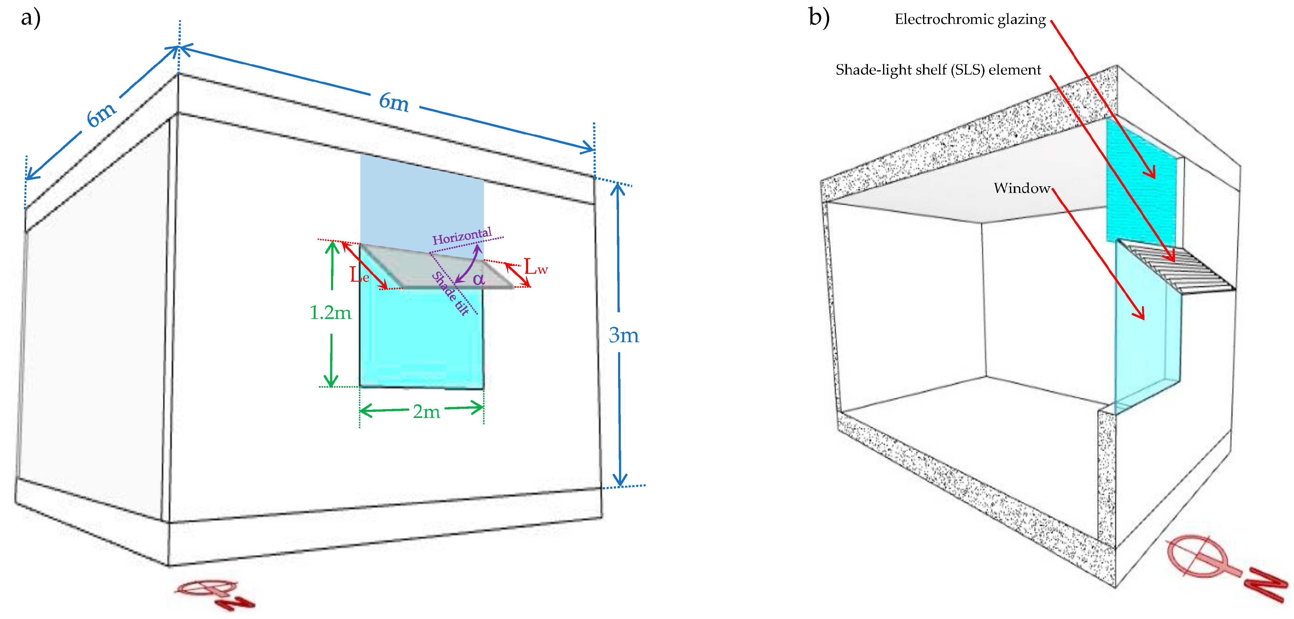
To find the optimum shade–light shelf system, which is named SLS hereafter, the authors directed yearly energy and comfort simulations based on a generic living space model, displayed in Figure 2, followed by a series of controlled experiments based on the optimum range solutions. The location of each simulation’s scenario was in Sydney, NSW, Australia. The simulations were performed for a north-facing window, which was the most dominant penetration in the southern hemisphere. The Pareto Front extracted from the simulation fed the field measurement, as described by Loftness and Hasse (2013): “Both simulation and measurement techniques are critical for ensuring the highest level of daylight quality, solar heat management, and views” [11]. The window sizes were determined based on data published by the Commonwealth Scientific and Industrial Research Organisation (CSIRO) and local window layout optimization research [42]. According to CSIRO, an average Window-to-Wall Ratio (WWR) of 23.96% was reported for all dwelling types in NSW [43]. Therefore, the case window for this study was based on a window of WWR = 25%. According to CSIRO, 68.03% of NSW dwelling windows have a U-val of 6 (W/m².K), and 56.57% have a Solar Heat Gain Coefficient (SHGC) of 0.6 [43]. Since Sydney, NSW is not a region with high heating loads, low SHGC glazings can contribute to thermal comfort [7]. Hence, the mentioned properties were considered for simulations and experiments (

Table 1. The parameters applied in the simulations.

Variables Affect the Thermal and Lighting Performance of the Room
Room dimensions		Length	Width	Height
		6 m	6 m	3 m
Climate		Location	Latitude	Longitude	Time zone	Elevation
		Sydney, NSW, Australia	33.83	151.07	GMT+10.0	4.00
Construction		Thickness	Thermal Conductivity	U-value
	Wall	0.12 mm Insulation + 78 mm solid wood + 13 mm gypsum	0.03 [W/m·K]	0.264 [W/m2·K]
	Roof	0.40 m	0.027 [W/m·K]	0.15 [W/m2·K]
	Floor	0.15 m screed with insulation + 0.14 m wood	0.115 [W/m·K]	0.18 [W/m2.K]	Reflectance factor
					0.2
Window		Visible Light Transmission	U-value	SHGC	Frame conductance
		68 [%]	6.7 [W/m2·K]	0.70	5 [W/m2·K]
Parameters in EnergyPlus Engine Simulation
		Equipment	12.0 [W/m2]
		Hot water	off
Ventilation		Wind-driven flow	off
		Buoyancy-driven flow	off
		Natural ventilation	on
		Scheduled ventilation setpoint	18 °C	Humidity air change	0.6 [ACH]
		Infiltration	0.5 [ACH]
		Humidity control	on
		Mechanical ventilation	on	Fresh air	8.33 [L/s/person]	Heat recovery	Sensible (0.6)
Heating		Constant setpoint	19 °C	Max. supply air temp.	30 °C	Heating limit	100 [W/m2]
Cooling		Constant setpoint	26 °C	Max. supply air temp.	18 °C	Heating limit	100 [W/m2]
People		People density	10 [m2/person]	Metabolic rate	1.2 [met]
Lighting		Lighting power density	12.0 [W/m2]	Illuminance target	500 [lux]	Dimming	stepped
Schedule

).

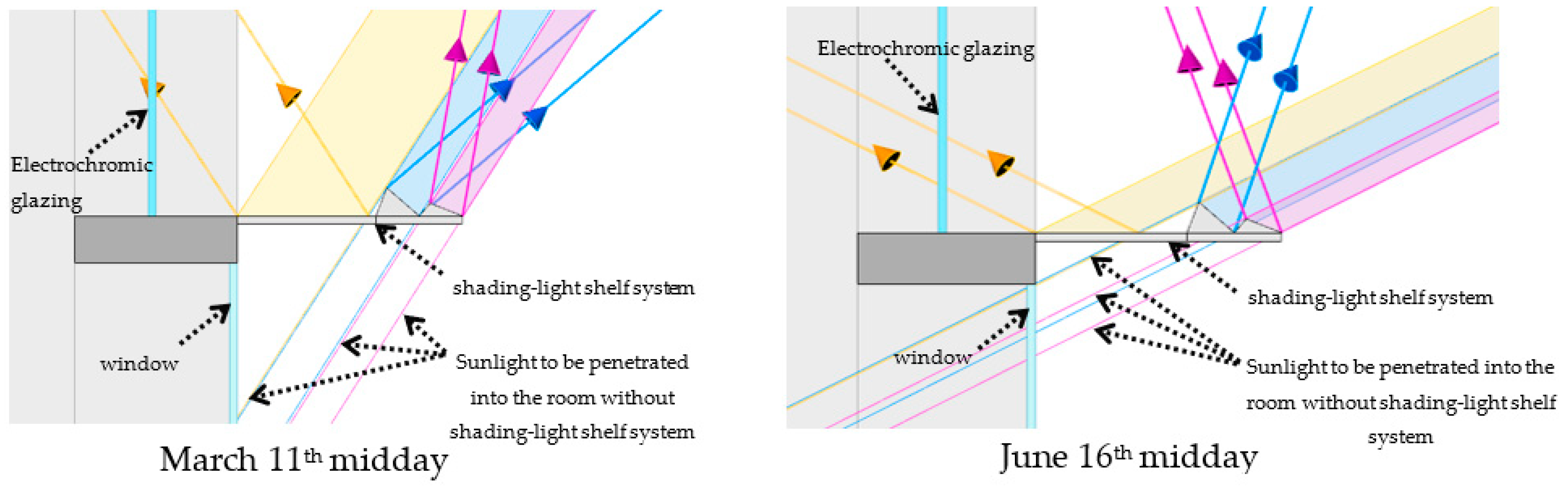
The daylight penetration was divided into two parts, an electrochromic area (on the top) and ordinary glazing (at the bottom—Figure 2). When the reflected sunlight off the top side of the SLS element is high, the electrochromic glazing changes its level of tint, moderating penetrated reflecting sunlight into the room.

According to the literature, for east and west-oriented penetrations, the most effective shade is fin (vertical shade) because of the extreme sun angle [27], due to the Sun’s path and altitude, overhang (horizontal shade) is the most suitable option for north-facing windows in the southern hemisphere. Hence, a moveable parametric horizontal shade was assumed in this research (Figure 2).

The active hours considered in the simulation and the following experiment were 8:00 a.m. to 6:00 p.m., Monday to Sunday, as the shading system’s effective hours were when the Sun casts light on the building. The occupancy hours, lighting, and appliance have been adopted from the calculations performed by Ahmed et al. [44]. Table 1 shows the simulation parameters and boundary conditions.

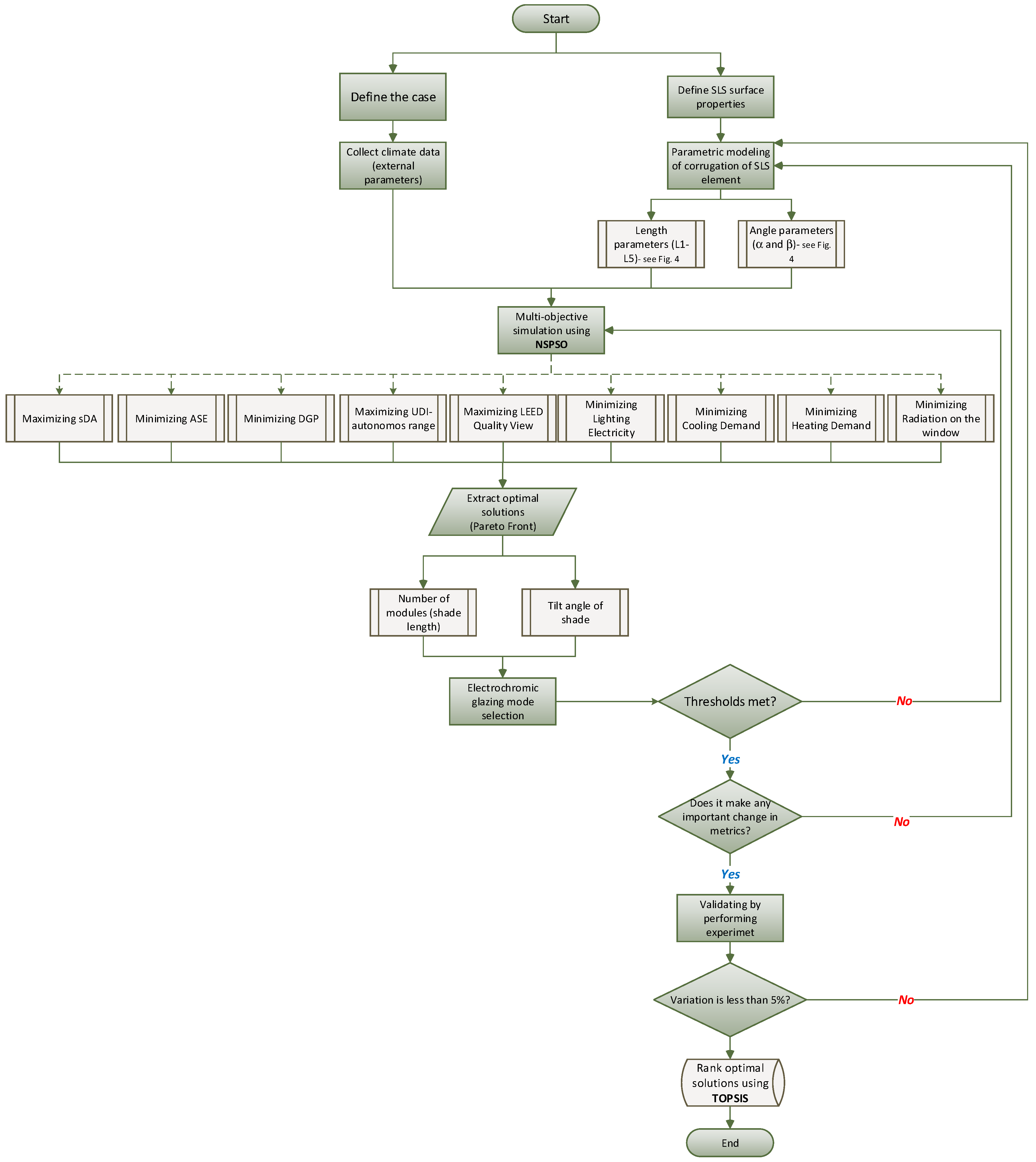
The authors conducted a yearly energy consumption (cooling load and lighting) and visual comfort simulation based on a single-floor dwelling, as shown in Figure 2. According to CSIRO, 57.07% of the cooling system in NSW is a non-ducted air-conditioner [45]. Therefore, this project’s heating and cooling system is an inverter air-conditioner. Figure 3 demonstrates findings for the optimum solution flowchart.

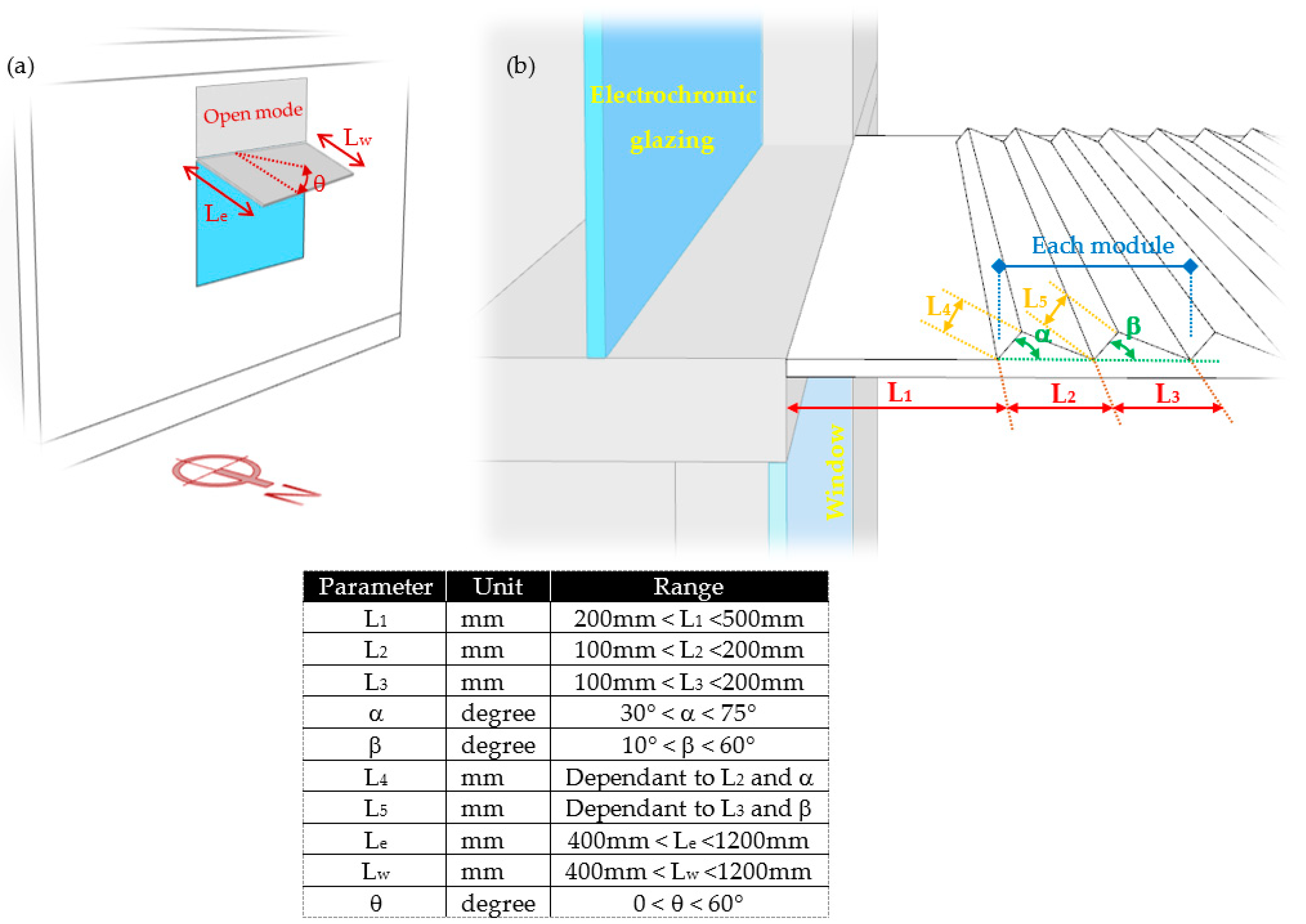
A preliminary simulation analysis of the reflectance, mirror properties, and optical characteristics of shading surfaces subjected to the Sun’s angle of incidence showed that a plastic material with white DuPont coating demonstrates the best performance. Reflectance of 80.88%, specular reflection of 0%, and diffusion of 80.88% were the selected properties for shading elements in shape optimization and field experiments. Firstly, a parametric simulation was performed to discover the optimum surface profile of the shade–light shelf element (Figure 5). The obtained near-optimum solutions were used as the final options and used in an experiment for one year to validate the simulation results.

Following the simulation and after extracting the optimum solution range (including eight optimum solutions for the whole shade length and inclinations), the experimental study was conducted to validate the simulation results. Two identical case rooms were used for field measurement. For one of the rooms, the near-optimum shade was prototyped using plastic-coated cardboard and installed on the room window facing north. The measurement equipment (see Table 3) was used in both rooms to assess objectives for one year. Through validating simulation results by experimenting with real conditions, a final algorithm for the shading mechanism was developed.

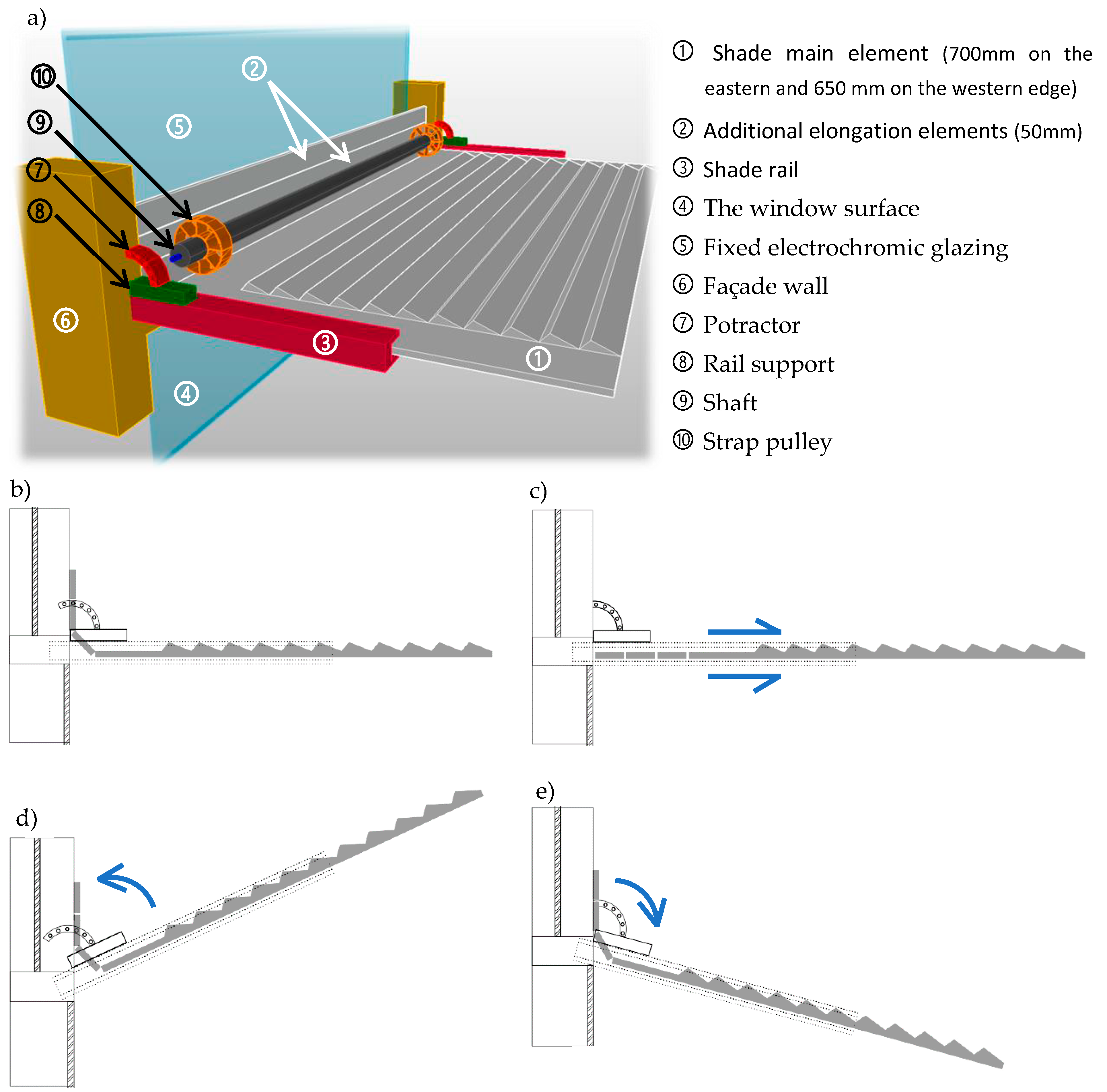
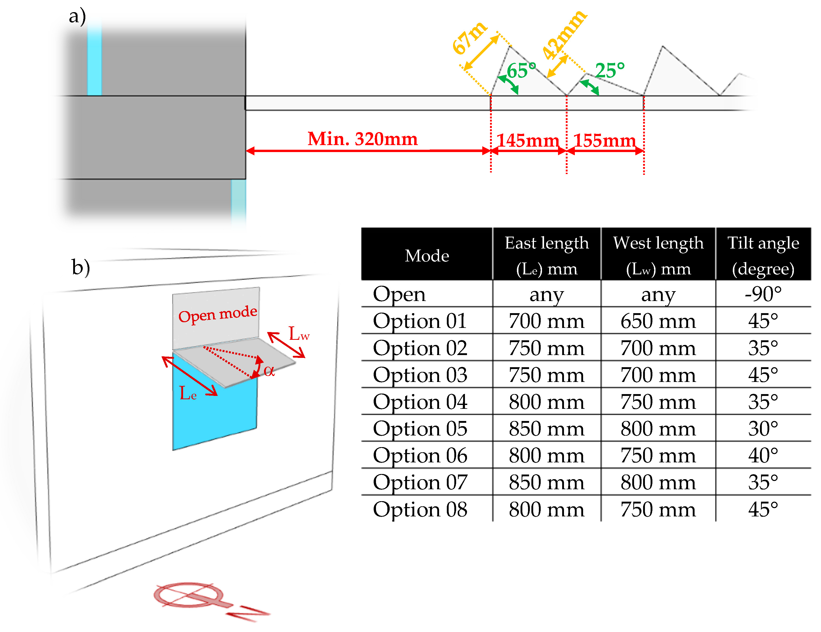
The shading system designed in this research works like the roller garage door and includes a main part of a 700 mm shading element and three additional modules of 50 mm. The reason behind choosing these dimensions was the simulation and experimental results (see Figure 3), which showed that the optimum shading length (regardless of angle) was between 700 mm and 850 mm. A protractor can incline the shade rail in an increment of 5° between 35° and 45° controlling the inclination angle of the rails (Figure 4). The Open mode for shade is the minimum length and 20° upward (Figure 4c).

The multi-objective optimization was performed entirely through Non-Dominated Sorting Swarm Particle Optimization (NSPSO), which is based on the evolutionary algorithm to modify PSO for better dominance comparison. Compared to similar algorithms, NSPSO uses a larger population size and provides “fast and better convergence towards the global front”. The algorithm (Algorithm 1) to implement NSPSO is as follows [46]:

Algorithm 1 NSPSO optimization pseudo-code.

1.  Initialize the population and then store it in a PSO_List:  1.1. Iteration counter t = 0;  1.2. Xi and Vi are the current positions, and velocity of the i-th particle is initialized randomly;  1.3. Pi is the best personal best position, which is set to Xi;  1.4. Wmax is set to the upper and lower bounds of the decision variable range;  1.5. Evaluate each particle.  2.  t = t + 1.  3.  Identify particles that offer non-dominated solutions and then store them in ND_List.  4.  Calculate niche count/crowding distance for each particle.  5.  Re-sort the ND_List according to niche count/crowding distance.  6.  For i = 0:  6.1. For the i-th particle, select a global best Pg randomly from the top 5%;  6.2. Calculate new Xi and Vi;  6.3. Add the i-th particle’s Pi and Xi to a population list of TP_List;  6.4. If i < number of particles:  6.4.1. Go to 6.1.  7.  Identify particles from TP_List.  8.  Empty PSO_List and repeat 2.  9.  If PSO_List size < number of particles:  9.1. Loop.

3.1. Simulations

Due to simulation tools, researchers can analyze different design schemes and manifold modelling that are not easily experimental on an absolute scale [16]. The present study performed an extensive series of simulations using Non-dominated Sorting Particle Swarm Optimization (NSPSO), which upgrades PSO by “making a better use of particles’ personal bests and offspring for more effective nondomination comparisons” [46]. The energy simulation engine is globally validated: EnergyPlus^TM, which is a whole-building energy console-based simulation program, was used to simulate energy-related aspects [6]. ClimateStudio, which uses RADIANCE engine, a four-component dynamic climate-based model that analyzes daylighting through raytracing calculation, was used for the daylight simulation process. The luminous performance of the virtual model was evaluated using the raytracing method of RADIANCE, a dynamic climate-based model that analyzes daylighting through raytracing calculations. To analyze thermal performance and energy-related parameters, including lighting, heating, cooling, and Predicted Percentage Dissatisfied (PPD), the EnergyPlus engine was used. The simulation included a fine-detailed model of four natural daylight components: direct sunlight, indirect sunlight, direct skylight, and indirect skylight [6,42,47,48].

3.2. Decision Variables

To achieve indoor visual and thermal comfort as well as the visual connection to the outside, nine objective functions were considered for optimization, described in

Table 2. The objective functions to be optimized.

Variable	sDA	ASE	UDI (Autonomous Range)	DGP (Disturbing Range)	LEED View Quality-v4.1	Solar Radiation on the Window Surface	Lighting Energy	Heating Energy	Cooling Energy
Maximized/minimized	Max.	Min.	Max.	Min.	Max.	Min.	Min.	Min.	Min.
Maximum threshold	---	1000 (lux)	3000 (lux)	38%	---	---	---	---	---
Minimum threshold	300 (lux)	---	300 (lux)	---	75%	---	---	---	---
Time domain	h	h	h	h	h	day	day	day	day

.

The output of the optimization process would be the shade dimensions and tilt angle (Figure 5a) as well as the shade surface attributes (Figure 5b).

3.3. Metrics and Measuring Formulae

3.3.1. Daylight Metrics

According to Xue et al. (2014), the perception of uniformity is the primary factor in occupants’ sensation of daylight in residential spaces [1]. In this study, evenly indoor distributed sunlight was considered due to the need for artificial lighting by moving away from the window [13].

Spatial Daylight Autonomy (sDA)

Spatial Daylight Autonomy (sDA) examines the percentage of indoor space receiving sufficient daylight (min 300 (lux)) for at least 50% of the annual occupied time. Together with ASE, sDA builds a clear image of indoor daylight performance. sDA is a universal metric approved in LEED-v4 and IES-Lighting Measurement-83 standard [49] and methodically formulated as

$$\mathrm{sDA}=\frac{{{\displaystyle \sum }}_{i=1}^{n}I{T}_i}{n}\hspace{1em}\hspace{1em}I{T}_i=\left\{\begin{array}{c}0, I{T}_i<\tau t_y\\ 1, I{T}_i\ge \tau t_y\end{array}\right.$$

(1)

where:

For a given point i, IT stands for the occurrence number when sDA outstrips the illuminance threshold. τ denotes the transitory fraction threshold, and t_y is the annual date–time count [50]. According to LEED-v4.1, an sDA greater than 75% receives 3 credits [51].

Annual Solar Exposure (ASE)

ASE was calculated as

$$\mathrm{ASE}=\frac{{{\displaystyle \sum }}_{i=1}^n{x}_i}{n} x_i=\left\{\begin{array}{c}0; x_i<T_i\\ 1; x_i\ge T_i\end{array}\right.$$

(2)

where:

x_i at the point i describes the incident number exceeding the ASE illuminance threshold (1000 (lux)), and T_i is the annual absolute hour threshold [50].

Useful Daylight Illuminance (UDI)

While sDA assesses daylight sufficiency, Useful Daylight Illuminance (UDI) attempts to separate too-bright situations that might result in visual discomfort. The daylight availability metric of UDI divided hourly time into three main categories: 0–100 (lux) (failing), 100–2000 (lux) (autonomous) (100–300 (lux) supplementary (may need additional artificial lighting); and 300–500 (lux): autonomous), and over 3000 (lux) (excessive) [52,53]. In this study, the “useful” range was optimized. Hereafter, in the manuscript, UDI means the autonomous range.

Daylight Glare Probability (DGP)

DGP evaluates indoor glare possibility. Whereas other glare indexes assess the subjects’ perception of glare, DGP expresses a probability that could result in occupants’ being disturbed by glare [54]. DGP is formulated as [54,55]

$$\mathrm{DGP}=\left(5.87\times {10}^{-5}{E}_V\right)+\left(9.18\times {10}^{-2}{\log }_{10}\left(1+{{\displaystyle \sum }}_{i=1}^n\frac{L_{s,i}^2\ast {\omega }_{s,i}}{E_V{}^{1.87}\times P_i^2}\right)\right)+0.16$$

(3)

where:

• E_V is vertical eye illuminance (lux);
• L_s,i is the luminance of ith-window (cd/m²);
• ω_s,i is the solid angle (angular size of the window seen) of ith-window (sr);
• P_i is the position index of the ith-window.

In this study, the authors analyzed glare probability for seated and standing positions.

3.3.2. Visual Connection (View)

A crafted shade can block out the sunlight, preventing overheating while supporting up to 80% visual contact [7]. In this study, the authors assessed both seated and standing occupants’ views.

Quality View

According to LEED View Quality-V4.1, at least 75% of the regularly occupied space area must have a direct view of the outdoor natural or urban environment. This view “must include at least one of the following: nature, urban landmarks, or art; or objects at least 7.5 m from the exterior of the glazing”.

3.3.3. Solar Radiation and Energy Transmission

Solar radiation is the primary factor in moving shading adjustments [18] as there is a clear relationship between shade deployment and solar radiation [56]. Overheating is prevalent in sunny climates as a percentage of the incident sunlight is converted to heat through absorption [7].

In climates such as Sydney, adequate daylight should be penetrated “without exceeding a maximum total solar energy transmission of 10–12%” [11] by obstructing the abundant daylight. It must be noted that the eave or overhang underside, if it exists, could act as a reflective surface, increasing overheating indoors, which was not considered in this study.

Finally, it worth mentioning that the energy for moving the system could be provided by solar-powered off-grid lithium ion battery to burden no more load on the building electricity consumption.

4. Results and Discussion

To assess the effect of the shading system on seven metrics and find the optimum options, a set of 4500 possibilities of shading length and inclination (in increments of 10 mm and 1°) were simulated on a yearly basis. To carry out a careful analysis, the authors conducted an intensive study on the effect of the optimized solution (Pareto Front solutions—see Figure 11) on sunlight admission for every hour of one year. Results of the one-year energy consumption, thermal and visual comfort simulation for the eight scenarios (Pareto Front solutions) were inputted into a sensitivity analysis.

Since this is a dynamic device, the blocked sunbeam could result in overheating and glare. Therefore, it should be optimized hourly or seasonally instead of using annual matrices. Two examples of the study are shown in Figure 6. Here, the beforementioned optimized corrugated surface fed the optimization process finding the optimum range solutions as the final options. The final options are presented in terms of the shade-light-shelf length (number of modules) and the tilt angle.

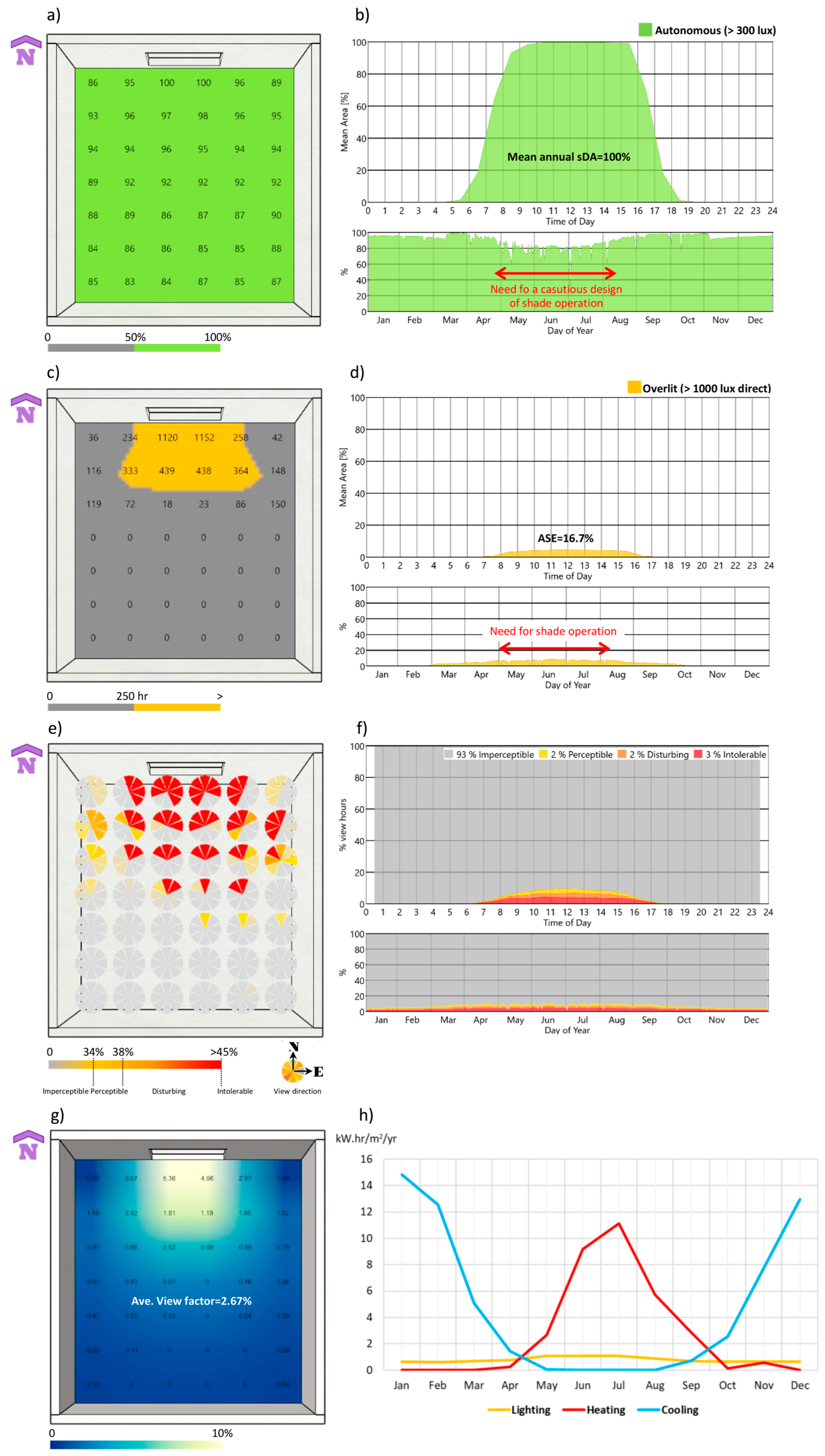
Results showed that the no-shade window admitted sufficient daylight, which means no need for artificial lighting (Figure 7a,b); though causing overlighting 42% of the near-window area receives excessive daylight (Figure 7c,d), which resulted in disturbing glare (Figure 7e). The operation of the shading system needed to efface overlighting. In addition, since sDA decreased from May to July (Figure 7b), the shading system should be designed carefully. The frequency of excessive daylight happens from April to September (Figure 7d), so the shade-in-operation was assumed to moderate it. By comparing sDA and ASE, there was a contradiction in shading element operation from May to July, which made the design more complex.

Energy simulation showed that for the no-shade state of the window, Energy Use Intensity (EUI) was 27.09 (Kw·hr/m²/yr) (Figure 7h), Operational-CO₂ Emissions was 11.41 (kg/m²/yr), and the Predicted Percentage of Dissatisfied (PPD) was 13.45%.

Hereafter, W_h represents window height. There was a fundamental contradiction (inverse relationship) between the shading effect on glare (with the steepest gradient), illuminance, and view. The greater the shade length or the higher the inclination, the less DGP (Figure 8), illuminance, and view. Changing the shade inclination from a horizontal state to 45° caused a decrease of 70.9%, 58.3%, and 10% in sDG, ASE, and view, respectively, and an increased in UDI of 12.3%, which was the direct result of eliminating excessive daylight. The minimum view for the most extended and slanted shade was 71.4%. To meet the minimum view quality, shade with a length of more than 90% W_h and an angle of more than 41° were excluded.

Changing the shade length from 30%W_h to 50%W_h decreased sDG, ASE, and view by 60.7%, 48.7%, and 12.4%, respectively, while increasing UDI. Confining Sdg < 40%, excluded horizontal shade of less than 19.3% vertical projection area of shade on the window surface. Restraining ASE < 10%, excluding the shade length of less than 43%W_h and inclination of less than 15°.

A thorough hourly analysis for every hour of daytime was carried out to show the effect of any length and inclination of shade on the metrics and measures. An example of this in-depth analysis performed on 19 March under clear sky conditions is illustrated in Figure 9 and Figure 10. The time lag due to the latent heat flux was also considered to estimate the loads.

Extending shade length from 33%W_h to 100%W_h decreased cooling load by 22.3% while increasing heating and lighting load by 36.2% and 260.1%, respectively. It means the longer the shade, the higher the heating and lighting demand. Tilting the shade from a horizontal state to 45° decreased cooling demand by 8.4% and increased heating and lighting by 308.6% and 53.6%, respectively. This fact accelerated finding the optimum shade modes, and effectiveness could be achieved more through optimizing the length.

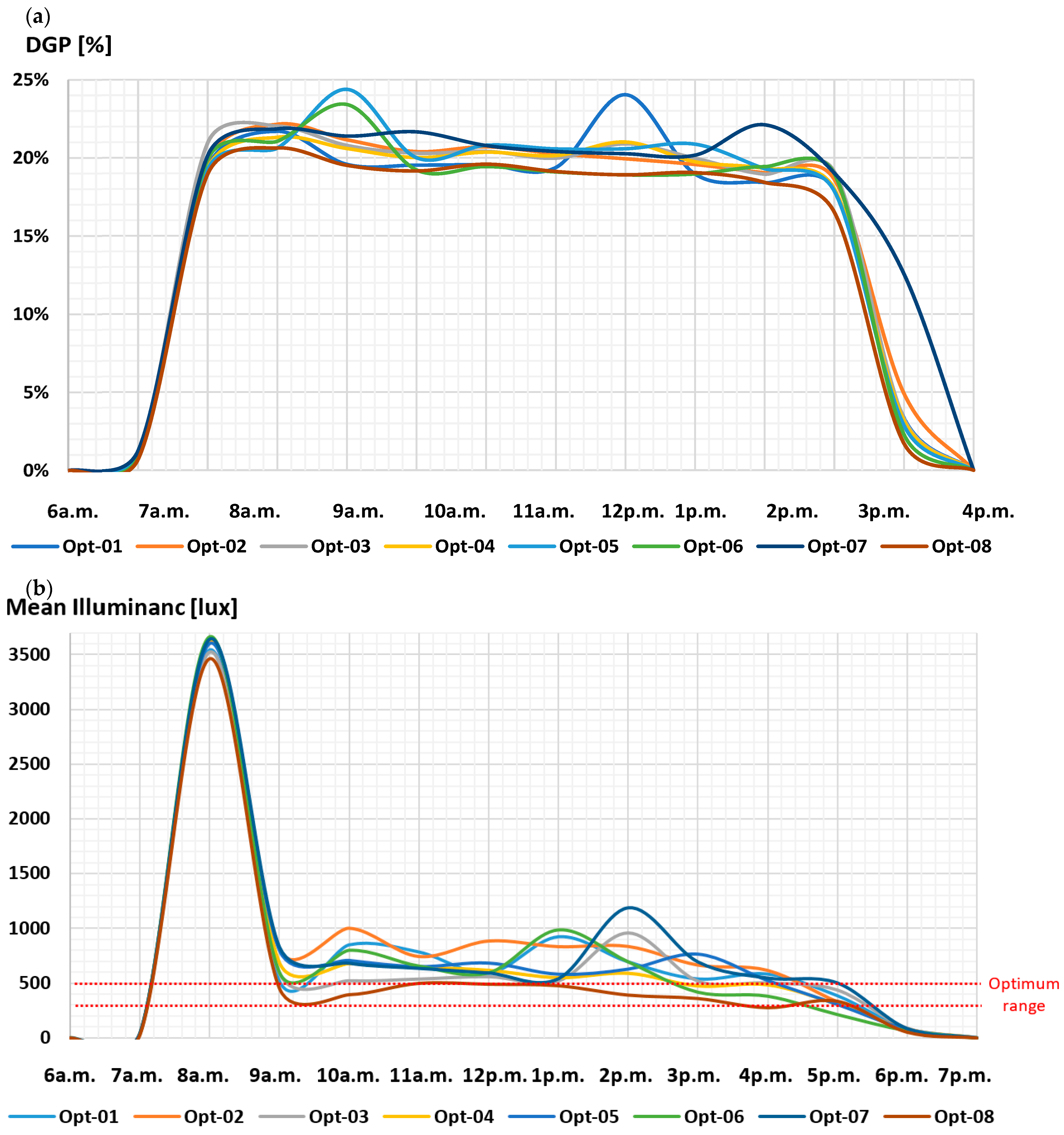
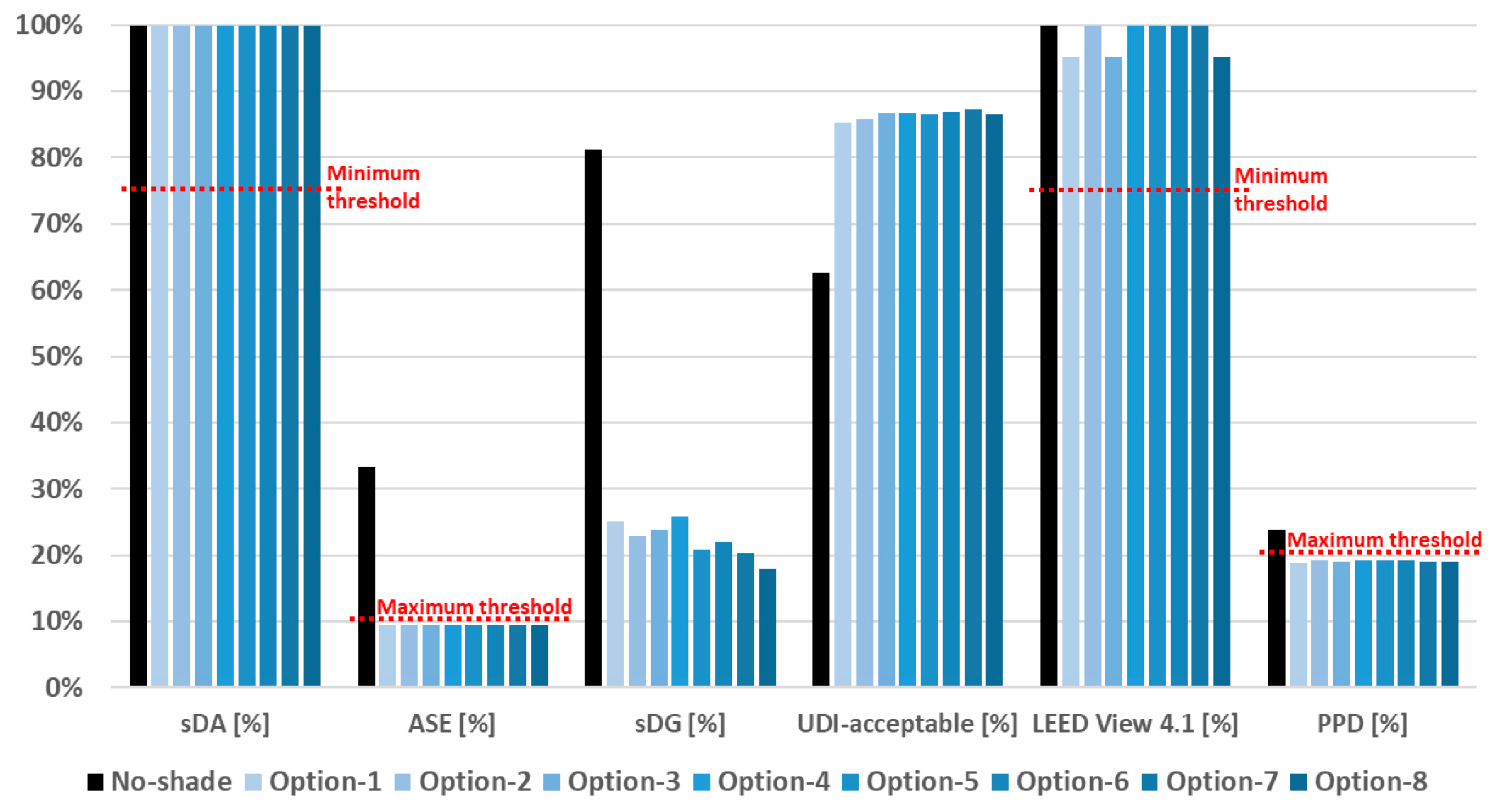
Contemplating sun position and local weather records, eight final optimized options were extracted from Pareto Front (Figure 11a). To order the preference-extracted options satisfying the multi-objective decision-making, we used the TOPSIS (Technique for Order of Preference by Similarity to Ideal Solution) technique.

All available operation strategy options guarantee the availability of 100% spatial daylight autonomy, which is equivalent to having no shading at all. Regarding indoor overlighting, all strategy options result in an average decrease of 70% in annual sunlight exposure (ASE) while keeping it below the maximum threshold. By optimizing shade position and attributes based on Sun position, adapting operational strategies for optimized shading reduces the probability of daylight glare by at least 78%. Additionally, all options increase acceptable useful daylight illuminance by at least 36%, which reduces the need for artificial lighting during the daytime. With respect to visual connection to the outdoors, only two options decrease the view by 5%, while all other options preserve the view. Furthermore, implementing any of these options can improve indoor thermal comfort and maintain it below the threshold, while a no-shade window cannot. Figure 12 demonstrates the changes in visual and thermal comfort resulting from shading options.

Apart from ASE and sDA, which are assessed yearly, and view, which is independent of time, a monthly study on the effect of shading strategies on DGP and mean UDI is shown in Figure 13.

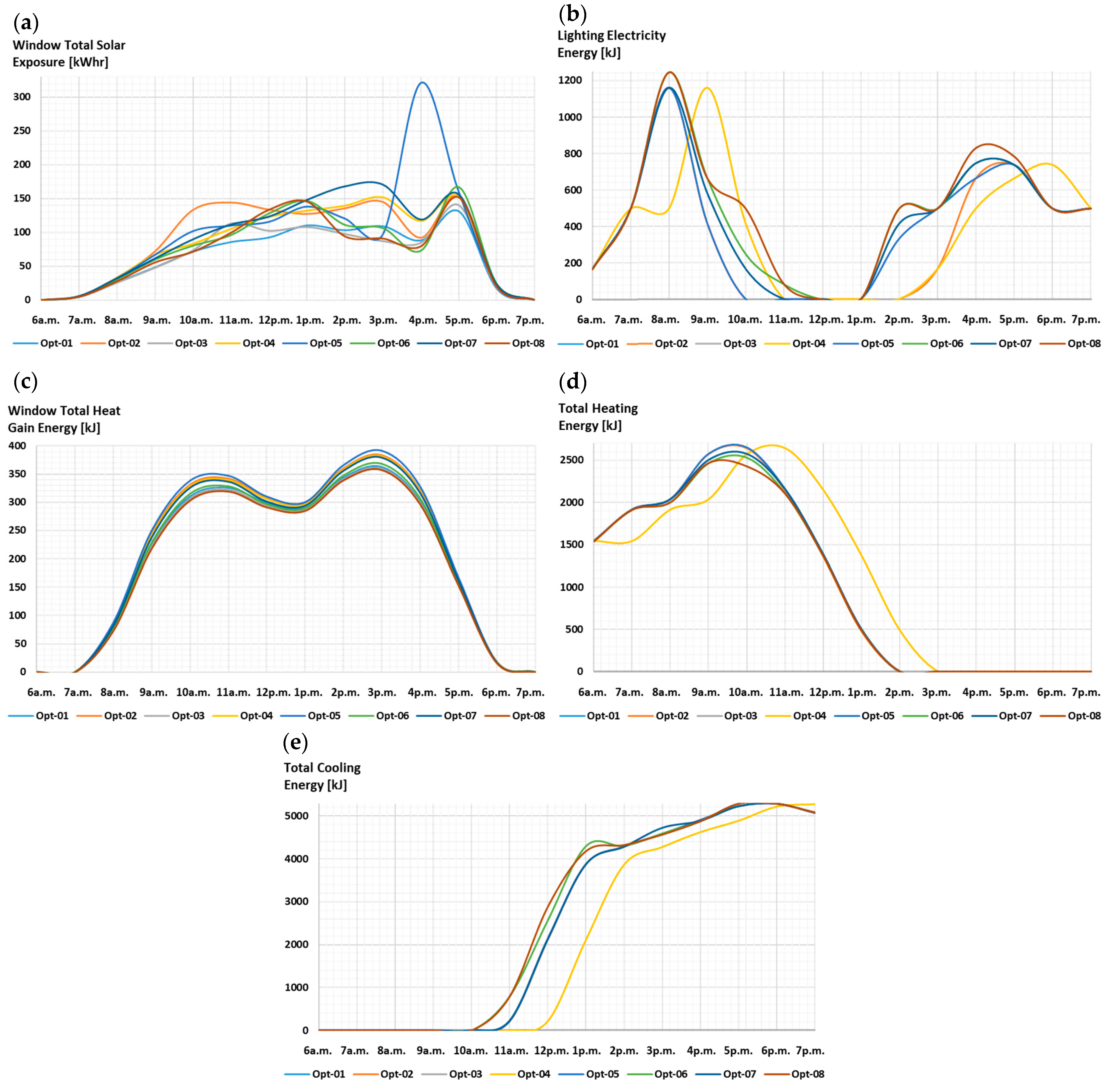
Converting energy used for lighting into heat, electric lighting could add up to 16% to the cooling loads [7,37]. Therefore, using shade increased lighting energy, which was insignificant compared to cooling energy savings.

In relation to solar radiation and its impact on no-shade windows, the study found that options 1 to 8 resulted in a reduction in solar radiation of 55.19%, 55.26%, 57.71%, 57.31%, 57.56%, 58.80%, 57.27%, and 60.22%, respectively. When considering the energy consumption aspect, implementing the shade led to a 14.1% increase in lighting energy, but did not significantly affect the heating load. This increase in energy consumption, however, was offset by a 78% reduction in cooling loads, as illustrated in Figure 14.

4.1. Validation of the Results

To establish the optimum shading strategies for different time and sky conditions, after numerical analysis and finding the optimum range of solutions, the authors built a prototype and then put it on the same windows shown in Figure 2 for one year. The shading element surface was built based on the optimization results (see Figure 11a). The shade could be extended or tilted manually. A metal bracket was used to sustain the shade. Two field measurement methods were employed to validate the optimized options. One is human subjects’ hourly declaration forms and recorded metrics by a network of sensors.

To see if the two methods gave the same measurement, the authors equipped the case rooms with sensors (

Table 3. The equipment for validating the results and providing the shade movement system with input.

Category	#	Equipment	Specification	Image
				Front	Back
Light and Illuminance measure	1	Grove© light sensor v1.2	- Peak wavelength 540 nm; - Response time 20–30 ms.
	2	Gravity© analog ambient light sensor	- Detecting range 1–6000 lux; - Response time 15 μs.
	3	Grove© luminance sensor	- Detecting range 0–1000 lux.
	4	Dr. meter© digital lux meter with remote sensor-LX1010B	- Detecting range 0–50,000 lux; - Accuracy ±4% rdg and ±0.5% f.s; - Sampling rate 2.0 times/sec.
	5	Tenmars© light meter-TM-202	- Detecting range 20–200,000 lux; - Sampling rate 2.5 times/sec; - Accuracy ±3%.
Angle and Length measure	6	Grove© infrared reflective sensor v1.2	- Effective detectable distance 4–15 mm; - Response time 10 μs; - Peak sensitivity wavelength 800 nm.
Temperature measure	7	Grove© temperature and humidity sensor (high accuracy) v1.0	- Humidity range 0–80% RH; - Detecting range 0–70 °C; - Temperature accuracy ±0.5 °C.
	8	Grove© infrared temperature sensor	- Ambient detecting range −40 to 85 °C; - Object detecting range −40 to 115 °C; - Measurement resolution 0.02 °C.
Move shade	9	Arduino© ABX00041Nano motor carrier	- 3V digital/analog sensor input/output; - Power terminal XT-30 and 2POS terminal block.
	10	Grove© I2C Motor Driver (TB6612FNG)-stepper motor control	- Driver IC for DC motor and stepper motor with output transistor in LD MOS structure with low ON-resistor.
View assessment	11	Sony© fisheye converter SEL057FEC	- 16 mm angle of view; - Max. magnification ratio 0.14×; - Angle of view (APS-C) 105°.
Glare evaluation	12	Raspberry Pi© HQ Camera	- Sensor back-illuminated sensor 12.3 megapixels; - Pixel size 1.55 μm × 1.55 μm; - Integrated IR cut filter.
	13	Raspberry Pi© Camera Module 2	- Still resolution 8-megapixel sensor; - Sensor resolution 3280 × 2464 pixels; - Horizontal field of view 62.2°.
Radiation measure	14	FLIR© C5 compact thermal camera	- Accuracy at ambient temp. 15–35 °C and object temp. 0–100 °C: ±3 °C; - 160 × 120 (19,200 pixels); - Multi-Spectral Dynamic Imaging; - 5-megapixel visual camera.

) that were matched at the same network assumed in the simulation. The location of the sensors in the actual experiment was matched with those used in the simulation process. In Figure 7, each dot represents the position of a sensor.

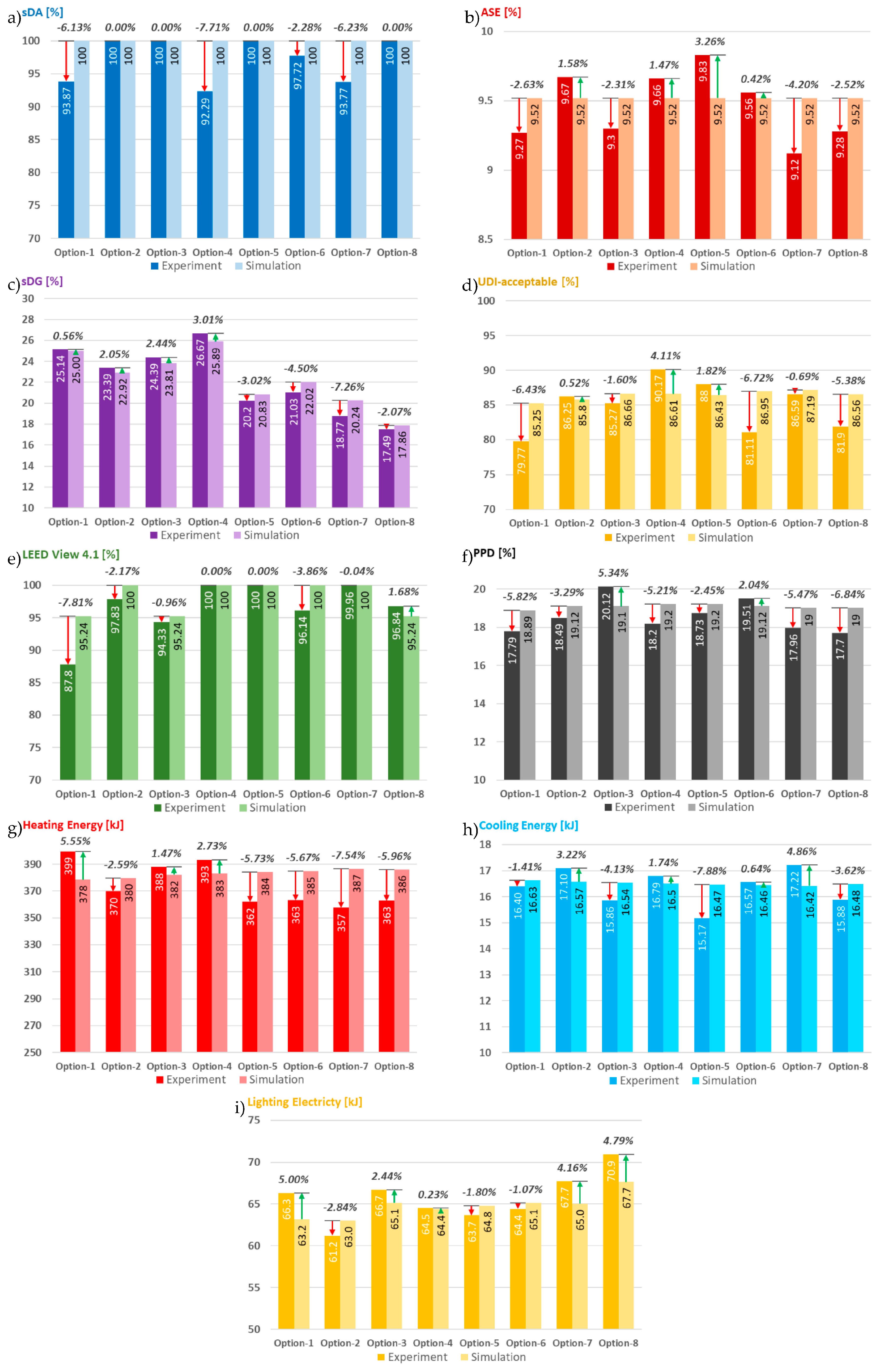
The recorded results show an average variation of 5.58% in sDA (Figure 15a); 2.29% in ASE (Figure 15b); 3.11% in sDG (Figure 15c); 3.40% in UDI (Figure 15d); 3.30% in Leed view-v4.1 (Figure 15e); 4.55% in PPD (Figure 15f). The energy consumption gauge demonstrated variations of 2.5%, 4.46%, and 3.41% in lighting (Figure 15g); heating (Figure 15h); and cooling demand (Figure 15i) relative to simulations.

The experimental validation of sDA revealed that variations in recordings mostly occurred for options in which the shade inclination tilt angle was near the maximum. This could be attributed to the shadow casting from shade elements on the sensors and illuminance meter, which were not accounted for during the simulation process. Moreover, the differences between the simulated and measured sDA and ASE could also be due to partial shading caused by tall trees (within 10 m) around the case room. The same issue was observed in the UDI assessment. The authors plan to investigate the impact of local tree shading combined with external dynamic shading elements in future research. The differences in sDG were not significant, except for option 7, which had the longest shading element. This difference could be attributed to the discrepancy between human visual perception and camera capabilities, as cameras may identify any sunbeams near the edge of the shading element as glare. The deviations between the simulation and experimental results for view and PPD could be attributed to individual differences in human subjects’ perception, which can vary slightly from the average. Finally, the slight variations in the summoned energy could be interpreted as the effect of latent heat flux.

4.2. Development of Shade-Activating Algorithm

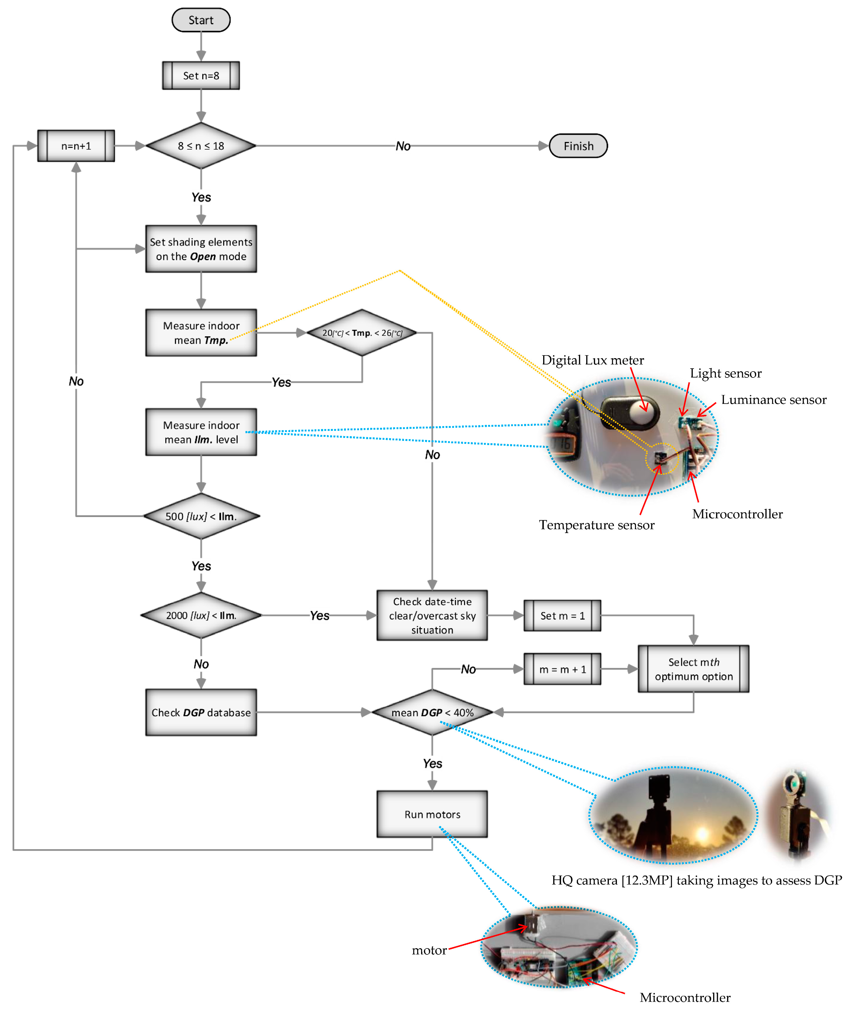
Finally, to design and implement the motorized shade, a network of sensors at a network of 1 m × 1 m, including six light sensors (Table 3—items 1–3), a temperature sensor (Table 3—item 5), and HQ cameras, was set up in the room to provide the automatic shading system with input.

After establishing the near-optimum options according to their performance and following the validating experiment, a block diagram for the operation of the shading system was developed (Figure 16).

5. Conclusions

The objective of this research is to enhance the effectiveness of a dynamic external shading system for north-facing windows in Sydney, Australia. The system automatically responds to indoor comfort conditions in eight predetermined scenarios. The study involved the simulation of numerous states for an external horizontal shade on north-facing windows to identify shading options that maintain indoor comfort while reducing Energy Use Intensity and operational CO₂ emissions. The researchers identified eight near-optimal shading options and tested them under similar yearly conditions using human subject assessments and sensor data capturing to validate the simulation results. The study found a high degree of accuracy, with an average variation of only 3.17% between field measurements and simulations.

The researchers simulated 4500 possibilities of shading length and inclination on a yearly basis to assess the shading system’s effect on seven metrics and find the optimum options. Implementing the optimized shading system had numerous positive impacts, such as eliminating overlighting, overheating, and glare. It also reduced solar radiation by 57% and cooling demand by 71%. However, some negative effects were observed, including a decrease in view quality by an average of 1.78%, a 23% increase in lighting electricity demand, and a 0.8% increase in heating demand. Overall, the designed shading system effectively maintained other visual and energy consumption indicators within acceptable ranges.

To validate the optimized options, two field measurement methods were used. The first involved human subjects’ hourly declaration forms, while the second utilized recorded metrics by a network of sensors. The researchers recommended an affordable field measurement system consisting of sensors and a camera to provide the microcontroller with data to operate the shading system automatically without the occupants’ intervention.

It is important to note that this study did not examine shading effects for all orientations and did not consider the impact of surrounding trees.