Article

Building Energy Performance Modeling through Regression Analysis: A Case of Tyree Energy Technologies Building at UNSW Sydney

1
School of Civil Engineering, The University of Sydney, Sydney, NSW 2008, Australia
2
School of Built Environment, The University of New South Wales, Sydney, NSW 2052, Australia
*
Author to whom correspondence should be addressed.
Buildings 2023, 13(4), 1089; https://doi.org/10.3390/buildings13041089
Submission received: 29 March 2023 / Revised: 16 April 2023 / Accepted: 18 April 2023 / Published: 20 April 2023
(This article belongs to the Special Issue Energy Efficiency and Carbon Neutrality in Buildings)

Abstract

:
Addressing clients’ demands, designers have become increasingly concerned about the operation phases of buildings and, more specifically, energy consumption. This issue has become more prominent as people realize that the Earth’s resources are limited and depleted, and buildings are major energy consumers. Building Information Modelling (BIM) has gained popularity in recent years and is now widely used by architects, engineers, and construction teams to collaborate and provide a comprehensive design that follows a sustainable strategy. The objective of this research is to examine how building variables are linked to energy consumption in various building shapes, achieved by building prototypes. The accuracy of the regression models is evaluated by undergoing a validation process. Consequently, this study created building information models of selected education facility office rooms and used Autodesk Insight 360 and Green Building Studio (GBS) to perform energy simulations. A 6 Green Star education building in Australia is chosen as the case study of this paper. Thirteen variables related to building internal design were examined, and five were found to endure a substantial effect on building energy consumption. The study also looked at the window-to-wall ratio (WWR), which was analyzed by multi-linear regression; however, the results showed that the model did not fit well, and the error obtained during the validation process ranged from 1.0% to 26.0%, which is unacceptable for this research. These findings highlight some limitations in using BIM tools and linear regression methods and discuss some potential improvements that can be achieved in future studies.

1. Introduction

1.1. Introduction

BIM provides a comprehensive platform for designers to gain a deeper understanding of the various building parameters to design buildings that are low in energy consumption [1,2].There are many tools on the market that use and are compatible with BIM technology, which facilitates designers from different fields. In addition, as an important part of statistics, regression models can provide a more significant indication of the dispersion and correlation of data. Combining the two allows designers to understand the parameters most critical to energy consumption. BIM is widely used by many companies, and a technical review of BIM applications suggests that two main considerations in BIM utilization are its compatibility with needs and its interoperability with other tools [3]. These two drivers can make BIM more useful to the community or industry. BIM integration with various tools and sources of data, such as building shape, geometry, materials, and equipment types, allows the creation of accurate energy modelling. Energy modelling practices are important since advanced models can be used to predict the energy consumption of various buildings. This outcome of simulations and estimations of energy consumption need to be compared with actual data acquired from energy meters or submeters recording the electrical, heating, ventilation, or air conditioning usage or the data collected and managed through building management systems in real time at smart buildings [4]. The validation of models using read data will eventually help to apply artificial intelligence (AI) algorithms to predict energy consumption and optimize energy efficiency based on changes in design variants, construction, or usage during the operation phase of the building [5]. Thus, the current practices of energy modelling are important to test or cross-verify the estimation methods for various design alternatives and shapes. This type of practice will eventually support advanced AI-based optimizations and predictions. Based on lessons from the current practices, AI will be further developed to automate the modelling process using big data created by numerous smart homes and buildings [4]. These modelling exercises, optimizations, and predictions are significant because they help facility managers and the building sectors to improve the energy performance, reduce greenhouse gas emissions, and contribute to sustainable development goals (SDGs), in particular, SDG 7, 11, and 13. These SDGs are respectively connected to the provision of modern and sustainable energy, the development of resilient and sustainable cities, and the implementation of urgent actions to combat climate change. The present paper on building energy performance modelling through regression analysis is very significant and relevant to achieving the SDGs. The study provides a means of evaluating and predicting building energy performance, which can contribute to reducing energy consumption, mitigating greenhouse gas emissions, and promoting green buildings or sustainable building design and operation practices. By investigating and improving energy efficiency in buildings, this study aligns with SDG 7 on affordable and clean energy, SDG 11 on sustainable cities and communities, and SDG 13 on climate action [6]; therefore, the current exercise is an important contribution to advancing sustainable development outcomes and addressing global challenges.

1.2. Problem Definition

As concerns about energy consumption have increased, standards have been specified to limit the energy consumption of buildings, such as the famous United States commercial building energy codes Standard 90.1 [7]. Furthermore, challenges such as the 2030 challenge have been developed to motivate designers to focus on the energy consumption of buildings [8]. Statistical methods have been popular since researchers are attracted to finding an easy way to evaluate building energy consumption. The statistical method provides a simple and accurate way to predict building energy consumption [9]. This paper aims to combine BIM technology and statistical methods to perform a further study of the ’building’s internal variables that affect the ’building’s energy consumption.

1.3. Objectives

There are four objectives that this paper aims to achieve. Firstly, the BIM models of six different shapes of offices in the building are created in Autodesk Revit. Using Revit allows users to develop a 3D solid model and modify building data efficiently [10]. Secondly, the energy simulation is developed in Autodesk Insight 360 and GBS. Thirdly, the statistical method is then used to investigate the relationship between selected building variables and energy consumption of six shapes of rooms separately. Furthermore, a validation is developed to obtain the error between simulation results and the one from a real-world case study. The Tyree Energy Technologies Building (TETB) of The University of New South Wales (UNSW) is chosen as the case study for this paper.

2. Literature Review

2.1. Implementing BIM in Green Building Design and Construction

2.1.1. Background of BIM Development in Green Construction

BIM was developed in the 1970s, but the promising concepts and values of BIM were agreed upon in 1999. Since this time, continuous efforts have been made to implement BIM in green building design. Succar revealed that BIM is comprised of interacting processes and technology, which can generate and manage building data throughout the entire project life cycle [11]. Abanda et al. then provided a list of 122 BIM software systems and indicated that the various functions of BIM can be competent in various aspects of green construction, such as building energy performance assessment, lighting analysis, and construction and demolition waste analysis [12]. Wong and Zhou presented a summary of literature reviews on BIM green construction but lacked the detail of specific frameworks to link BIM with green construction [13]. However, Lu et al. presented an essential assessment of the relationship between BIM and green buildings and proposed a Green BIM Triangle organization to conceptualize the interactions between BIM and green buildings.

2.1.2. Energy Simulation by BIM

BIM stores massive energy-related building information and has a strong capability for information exchange. It can extract all building geometry information from the architectural building model and forecast total energy consumption and make recommendations for energy optimization [14]. With these results, designers can build more sustainable buildings.
Kamel and Memari summarized previous case studies about the use of various BIM tools in energy analysis. These case studies indicate that the building models are mostly developed based on Revit or ArchiCAD [15]. Revit and ArchiCAD have strong conceptual massing capabilities, which can use basic shapes to model building form and orientation in the early design stage. The building energy model can be automatically generated from the building model through the prototyping of an Application Programming Interface (API). The user can update the design concept anytime in Revit or ArchiCAD and the energy model is also updated automatically. The two most prevalent BIM file schemas are gbXML and IFC, which allow data transfer. Feasible energy simulation tools are various, including EnergyPlus, OpenStudio, and GBS. They take either IFC or gbXML as the input to generate the building energy performance results.

2.2. Research Gap and Challenges for BIM-Based Energy Simulation

2.2.1. Limitations of Using BIM Tools

Kamel and Memari also investigated the feasibility of data exchange from BIM to BEM and found that the lack of interoperability was a major issue in implementing BIM tools [15]. Table 1 summarizes their findings in data transfer between different tools based on three case studies. Direct transfer from Revit to GBS is the most feasible and convenient solution, which is also applied in this study. Other BIM tools either have missing data or require manual input, which is not user-friendly. Secondly, today’s industry is lacking clear construction standards and codes for various aspects of the BIM application. Thirty-six existing standards of Green BIM application have been studied by Chong et al., but those standards do not pay much attention to the specific execution of BIM application in green building design, such as refurbishment and demolition of green buildings [16]. Lastly, low industrial acceptance of BIM technology is also an important issue. BIM is an innovative technology that requires collaboration among various software tools. The lack of knowledge and expertise in the industry makes workers rely on conventional construction methods [17].

2.2.2. Future Work Directions of BIM

According to the issues identified in Section 2.2.1, the process of data extraction and exchange needs to be optimized by enhancing the functionality of gbXML and IFC Schema. An efficient algorithm also needs to be developed to enable the automatic extraction of specific types of energy data from the BIM model. More compatible middleware is required to develop if direct data transfer is prohibited. Moreover, future research should pay more attention to the technical details of implementing BIM in energy simulation and all relevant green building designs rather than just making recommendations to use BIM. A complete industry standard of BIM application and a more effective framework for the energy simulation process is expected to be developed.

2.3. Multiple Linear Regression (MLR) Models of Energy Simulation

2.3.1. Background

As the building sector is the largest energy and CO2 emitter, energy prediction models have been researched and innovated over the past decades. In the early research, physical models with static energy analysis were first used to predict energy consumption, which is quite time-consuming and labor-intensive. Some mathematical models and energy forecasting software were then developed, which improve the prediction speed but cannot perfectly match the simulation data. Moreover, the involved mathematical formulas or programming language requires expertise [18]. Compared with various energy prediction tools, the multiple linear regression (MLR) models are the most appropriate prediction tool to be implemented in this thesis study due to its simplicity and high accuracy [19]. MLR can express the simulated energy data in a linear equation to predict the energy consumption of given material properties.

2.3.2. Application in Building Energy Simulation

Multiple regression models have been applied widely in different areas of energy analysis, such as residential building retrofit, heat load prediction and building energy usage estimation, etc. Walter and Sohn used a multivariate linear regression model to quantify the contribution of each building variable to the total energy usage. However, the model is not validated by the post-retrofit energy data [20]. Martinez et al. applied the same technique to assess the energy performance results of a residential house after retrofit and found that upgrading building envelopes increase energy savings [21]. Jaffa et al. also developed an accurate polynomial model summarizing the influence of heat consumption [22]. Lam et al. studied the energy consumption of office buildings in different climates in China. They imported 12 design variables, including building loads, HVAC system, etc., and surprisingly found that the difference between regression prediction and DOE simulation is within 10%. The result implies that the regression models developed can be used to estimate the likely energy savings or consumption during the initial design stage when different building schemes and design concepts are being considered [23].
Mottahedi et al. obtained a more accurate prediction with a maximum error of 5% on total energy consumption. The researchers made a multiple linear regression model to predict the energy consumption of an office building with seven different shapes [24]. The model includes the regression coefficient for each design parameter, and the format is also adopted in this study to generate an MLR model.

2.3.3. Limitations of Multiple Linear Regression Models (MLR)

The main issue of using a multiple linear regression model is the multicollinearity, which is caused by the high correlation among internal factors. Multicollinearity makes it hard to interpret the coefficients and thus reduces the capability of the model to present the effect of independent variables. Another issue is that MLR cannot perform accurate predictions as non-linear models produced by machine learning models, such as Artificial Neural Networks (ANNs) and Support Vector Machines (SVMs) [25]. This is because linearity cannot entirely represent reality, and the building model is so complicated that not every detail of the building can be modelled.

2.3.4. Future Work Direction of MLR

The MLR needs to be improved to detect the multicollinearity issue and illustrate the residuals from its best-fit regression equation. Moreover, the sensitivity analysis should be applied to aid in the regression approach as it can measure the relative standing of the effect limitations, making it possible to replace the design parameters that may influence an insignificant effect on the dependent variable. Moreover, the stepwise function can be used to determine whether to eliminate or add influence variables based on the level of correlation. However, the future trend should focus more on non-linear modelling to obtain more accurate forecast results. More machine-learning models should be introduced to the industries [25].

2.4. Energy Regression Analysis Combine with BIM Tools

2.4.1. Necessity for MLR Combine with BIM

Many case studies have indicated the applicability of BIM in energy simulation in Section 2.1.2, but few papers have verified the simulation results and tested their validity. The accuracy of the simulation is confronted by the challenge of interoperability issues among BIM tools. Interoperability refers to the ability of two or more systems to exchange information that is needed and available to use the information [16]. Several studies have summarized the potential issues of the two most proposed Data exchange Schemes (IFC, and gbXML). Choi et al. found that data loss frequently occurs when transferring IFC model data into the energy model, leading to incomplete or incorrect IFC files. Moreover, the definitions of IFC can vary with different BIM authoring tools, and thus unexpected errors were often created, reducing the reliability of results [26]. Pinherio et al. pointed out that the gbXML-enabled data exchange is inappropriate for large complex building shapes since the calculated surface areas and space volume differences might exceed the standard engineering tolerance and cause an overestimation of building energy consumption [27]. Moreover, the lack of the geometric representation of heating, ventilation, and air conditioning systems for gbXML might affect the simulation results [28].
These findings above indicate that the energy simulation process produces errors and thus, the model validation is necessary to decide whether the errors are within the acceptable range. Model validation can be achieved by constructing MLR with a series of statistical analyses, such as T-test, F-test, and ANOVA. MLR can predict the energy simulation results produced from the BIM energy analysis software and represent them in linear equations. The comparison between regression prediction and BIM simulation results can be visualized by generating bar plots on MATLAB.

2.4.2. Summary of Relevant Case Study

There is a lot of separate literature on regression analysis to predict energy use and BIM to simulate energy models, but few studies have mentioned how the two technologies work together. Table 2 below is a summary of case studies about the combination of these two techniques.

2.5. Comparative Study between Existing Building Energy Studies and IDEA Model

The traditional methods to explore building energy consumption mainly focus on fundamental data and lack interaction of influencing elements from both macro and micro levels [32]. However, an innovative energy simulation model was introduced by Huo et al. to investigate the carbon emission of Chinese commercial buildings toward 2060, which is the integrated dynamic emission assessment mode (IDEAM) [33]. The IDEAM consists of the system dynamics (SDs) model and a bottom-up end-use decomposition model, which can not only reflect the influential parameters but also provide an interactive feedback mechanism between different levels of parameters [33]. The IDEAM has been successfully utilized in exploring the interaction among different influencing elements and predicting the urban residential building’s carbon emissions [34].

2.6. Literature Summary and Critical Review

In this literature review, three articles provided the definition and wide application of BIM in green building constructions. One article identified that the energy simulation results obtained by BIM are comprehensive due to its rich database and information exchange capability. One article made a summary of case studies using BIM tools in energy analysis and found the two reliable modelling tools and file schemas used in data transfer. Three articles demonstrated three key limitations of using BIM, including the lack of interoperability, industry standards, and acceptance. It is thus recommended to develop an efficient algorithm or more compatible middleware to enable more efficient and accurate data transfer in the future. One article then summarized the traditional energy prediction methods and emphasized the ease of operation and precision for MLR through comparison. Five articles have applied regression techniques in various fields of energy measurements and found that most energy data can be verified by MLR. However, the multicollinearity issue is an inevitable challenge for MLR, and thus, one article suggests focusing more on non-linear model prediction and machine learning models in future work. The limitations mentioned above and findings from four articles indicated that BIM simulations would produce unexpected errors. Thus, it is necessary to combine MLR with BIM to validate the results.
Additionally, the innovation research method (IDEAM) that considers both macro and micro variables is compared with the traditional method; however, this article aims to explore the interaction between energy consumption and building internal variables, which are factors belonging to the micro level. The ambient influencing elements are ignored to simplify the whole process. Hence, the traditional fundamental study is more compatible with this research.
These articles have helped to deepen our understanding of the BIM concept, the breadth of its capabilities, and its distinct advantages over other analysis software. The articles on the application of BIM in the energy field provide a good theoretical basis for the methodology of this thesis. Although these articles also exposed some flaws and limitations of BIM, this thesis does not aim to solve these issues but summarizes the limitations during the energy simulation process.

3. Materials and Methods

3.1. Tools

Table 3 below illustrates the tools used in building BIM models and performing energy simulations.

3.2. Building Elements, Properties, and Energy Settings

Due to the limitation of information, only three building elements were used in the room models, and some types defaulted in Revit. Additionally, each room model has the same room area of 20 square meters to better prevent results from being influenced by too many independent variables.
Table 4 shows the energy setting used in this study. Due to the limited information available, most settings are set to default, while several of them were chosen accordingly.
Table 5 shows the material properties used in energy simulation, and these include the major building components such as roofs, walls, floors, and glass type. Different types are measured by U-Value, which indicates the thermal transmittance of the material [39].

3.3. Autodesk Insight 360

Autodesk Insight 360 is a cloud-based service that allows users to create different scenarios by changing the selected building parameters, such as building orientation, window shading, wall and roof construction type, and find out the best performance selection so that the most energy-efficient design can be generated [40]. In this study, Insight 360 was used as a preliminary analysis tool to provide the 3D analytical model based on the BIM models.
Insight 360 also provides the energy consumption required by the standard and the idealized design to better help users understand the parts that can be improved and realize the importance of designing energy-efficient buildings.
The six models of office rooms are displayed in the form of several surfaces with different colors. The interactive selection box allows the users to adjust the different building internal variables, including building orientation, Window-to-Wall ratio, window glass type, window shading, wall construction, roof construction, building infiltration rate, lighting efficiency, daylighting and occupancy controls, plug load efficiency, HVAC system, operating schedule, PV-Panel efficiency, PV-Payback limit, and PV-surface coverage. Figure 1 displays the analytical models of six different shapes developed in Insight 360. Each model is assigned a number, which is used to identify them in the following contents.

3.4. Autodesk Green Building Studio (GBS)
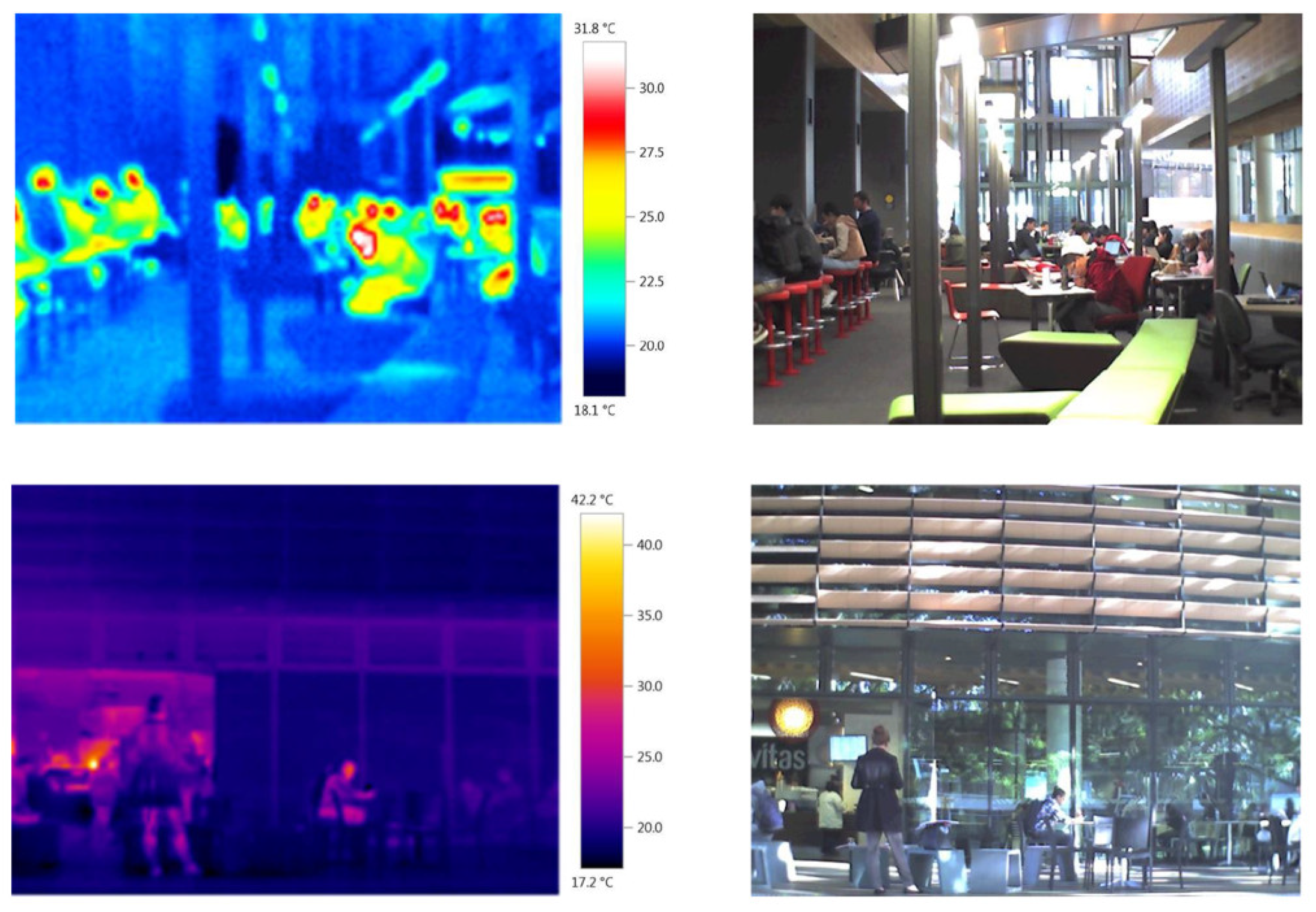
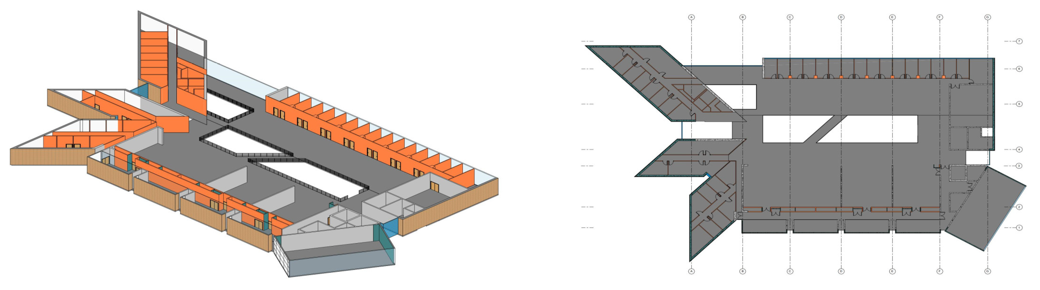
Similar to Insight 360, GBS is also a cloud-based energy simulation tool. GSB can develop and evaluate several building variables and run alternatives simulation automatically by changing building variables [38]. Additionally, GBS is the back engine of Insight 360. It provides computational support for Insight 360. Therefore, the building variables in both tools are highly matched. Furthermore, the energy simulation data can be exported as a CSV file, which allows users to develop statistical analysis in other programming tools.

3.5. Case Study

The Tyree Energy Technologies Building (TETB) is the case study of this paper. TETB is a 6 Green Star laboratory building in Australia. Figure 2 presents some images from two internal areas along with thermal images. The photos also show the students’ activities in those areas. This building is also used for teaching, meeting room, student group meetings, and studies. Thus, comfort, Co2, and temperature are critical factors for this building during operation.
Based on the introduction of Taylor Thomson Whitting (TTW), the Structural, Façade and civil engineering consultant of this project, several energy-saving technologies, such as the highly efficient Façade fabricated of glass and terracotta tiles, the featured steel roof span across the cantilevers over the entrances, makes this building not only full of technology and sustainable but also injected with research significance. In this research, six office rooms of TETB with typical shapes were chosen as the objects. Six shapes are extracted to allow researchers to find out the importance of different building variables in building energy simulation. The findings are compared with the original models to perform error analysis to corroborate the findings. Figure 3 and Figure 4 display the BIM model of TETB and the office rooms selected for this research.
This paper aims to investigate the relationship between building internal variables and energy consumption. The BIM models of seven different shapes were built in Revit. The energy simulations were performed in Insight 360, which allows users to compare the original design with various benchmarks. The alternative designs were developed by GBS automatically, and the detailed calculation data were exported as a CSV file for the statistical analysis discussed in the next section. Additionally, six real-world rooms in TETB were prepared in Revit to prove the statistical analysis developed in the next step.

4. Obtaining, Filtering Data, and Performing Statistical Analysis

4.1. Introduction

Statistical analysis was used to investigate how each building variable can affect energy consumption.
The six initial data sets were generated by GBS and exported as CSV files. The appropriate data filtering work is necessary for large data analysis. Dropping bad and unnecessary data during the filtering process can balance the trade-off between the filtered data size and the information preserved and attenuate the effect of excessively abnormal data on the sample [41].

4.2. Tools

The statistical analysis is performed in MathWorks MATLAB. MATLAB is one of the most popular technical computing tools in engineering and scientific areas [42]. MATLAB is a comprehensive and powerful data computing platform that is compatible with a wide range of file formats, including the CSV file format. Moreover, it comes with multiple toolboxes to allow users to handle large volumes of data and calculations. In this study, several built-in functions, such as “fitlm” and “corrcoef” are called to calculate the statistical indices and to help researchers understand the data distribution and linear relationships.

4.3. Building Variables

The building variables play important roles in determining building energy consumption. Only the internal building variables were researched because internal variables, such as wall construction type and infiltration rate, can be easily controlled by using different materials during the construction stage, and they are more stable once the building is built. GBS output files and previous studies from others determine the selection of building variables. Several papers by others have already illustrated the importance of several building internal variables on energy consumption, which are shown in Table 6.
According to other studies, building internal variables, including wall construction type, roof construction type, window-to-wall ratio, building orientation, infiltration, lighting efficiency, daylighting, and occupancy control, plug load efficiency, HVAC types, operating schedule, Min/Max internal loads, Min/Max envelope, and Min/Max form, were chosen as the independent variables in this study. Additionally, these parameters are also the design variables in GBS. GBS allows users to create alternative designs, which provides users with a convenient and straightforward way to analyze the relationships among them by changing these variables individually. Table 6 lists the selected variables and descriptions.
It is worth noting that not all the variables from GBS are within the scope of this paper. Based on the description in Table 6 and the box chart analysis in Section 5.2.1, the ORI has a very concentrated data distribution, suggesting that the ORI does not have a significant effect on energy consumption in this study, and it is discarded. In addition, although the HVAC system was considered a significant variable affecting energy consumption in other studies, the limited information available and that TETB, as a 6-star energy efficient building, makes extensive use of natural ventilation systems to reduce energy consumption, as well as the inability of GBS to fully output all internal variables of the HVAC system, led to the HVAC system being discarded in this study. Min/Max Internal Loads, Min/Max Envelop, and Min/Max Form are also discarded due to each with only two sets of available data and the inability to manually add design alternatives. Additionally, DOC and OPS are categorical variables and have no numerical meanings, which are discarded in this study.
There are several indicators provided by GBS to help designers evaluate building performance. These indicators include energy use intensity (EUI), electric cost, fuel cost, total annual cost, and total annual energy consumption. However, these variables, except EUI, are highly limited by building size and local currency and utility rates. Therefore, energy use intensity (EUI) is chosen as the dependent variable and indicator to evaluate building energy consumption.

4.4. Linear Regression Model

The regression method is a central part of many research projects and has been utilized in almost every field, including economics, biological science, and engineering [43]. The regression method provides users with a simple, efficient way to study the dependence, which can be understood if a result depends on other characteristics and how strong it is. Linear regression is the essential and most commonly used method in regression [44]. Previous research by others has validated the effectiveness of using linear regression methods to analysis building energy consumption [45,46,47]. Other researchers, such as Aydinalp-Kiksal et al., agreed that the regression method is easier to use without the specific expertise required [48,49]. This study aims to find the preliminary relationships between building variables and building energy consumption. These relationships can be explained as the dependence of energy consumption on multiple building variables. Therefore, the linear regression can summarize obtained data as simply as possible [44], which is highly compatible with this research.
Simple linear regression (SLR) can estimate the relationship between a single independent variable and a dependent variable by fitting the data with a straight line. The general formula is listed below:
y = α + β 1 x + ϵ
  • y is the predicted value of the dependent variable;
  • x is the independent variable;
  • α is the intercept, which is the predicted value of y when x = 0 ;
  • β 1 is the estimated regression coefficient, it decides the trend and the correlation strength between y and x ;
  • ϵ is the error of the estimate.
Apart from simple linear regression, multi-linear regression (MLR) is used to estimate the relationship between two or more independent variables and one dependent variable. The general formula is listed below:
y = α + β 0 x 0 + β 1 x 1 + β 2 x 2 + + β n x n + ϵ
  • y is the predicted value of the dependent variable;
  • x 1 ,   x 2   x n are the independent variables;
  • α is the intercept, which is the predicted value of y when x = 0 ;
  • β 1 ,     β 2   β n are the estimated regression coefficients, each of them decides the trend and the correlation strength between y and x individually;
  • ϵ is the error of the estimate.

4.5. Statistical Indicators

To understand the distribution and meaning of data, performing the statistical test is an essential step. The indicators help to understand the distribution, validity, and significance of data. Four statistical indicators: correlation ecoefficiency, root mean square error (RMSE), adjusted R-square, and p-value are selected in this study. These indicators are generated by the MATLAB functions and are used to evaluate the reliability of results.

5. Simulation Results

5.1. Introduction

The corresponding statistical analysis was developed based on the research above. The energy simulation results, as well as statistical analysis values and diagrams, are demonstrated in the following parts. The distribution and trends of data are also discussed. Seven BIM models of realistic rooms of TETB are used to verify the proposed regression models. The error analysis is performed to find out the accuracy of the proposed model regression models based on the Monte Carlo method. The relationship between several independent variables and dependent variables is discussed and summarized in the following sections.

5.2. Energy Simulation Results

This section displays data related to selected variables from GBS in graphical form. Both data filtering and statistical analysis were completed in MATLAB.

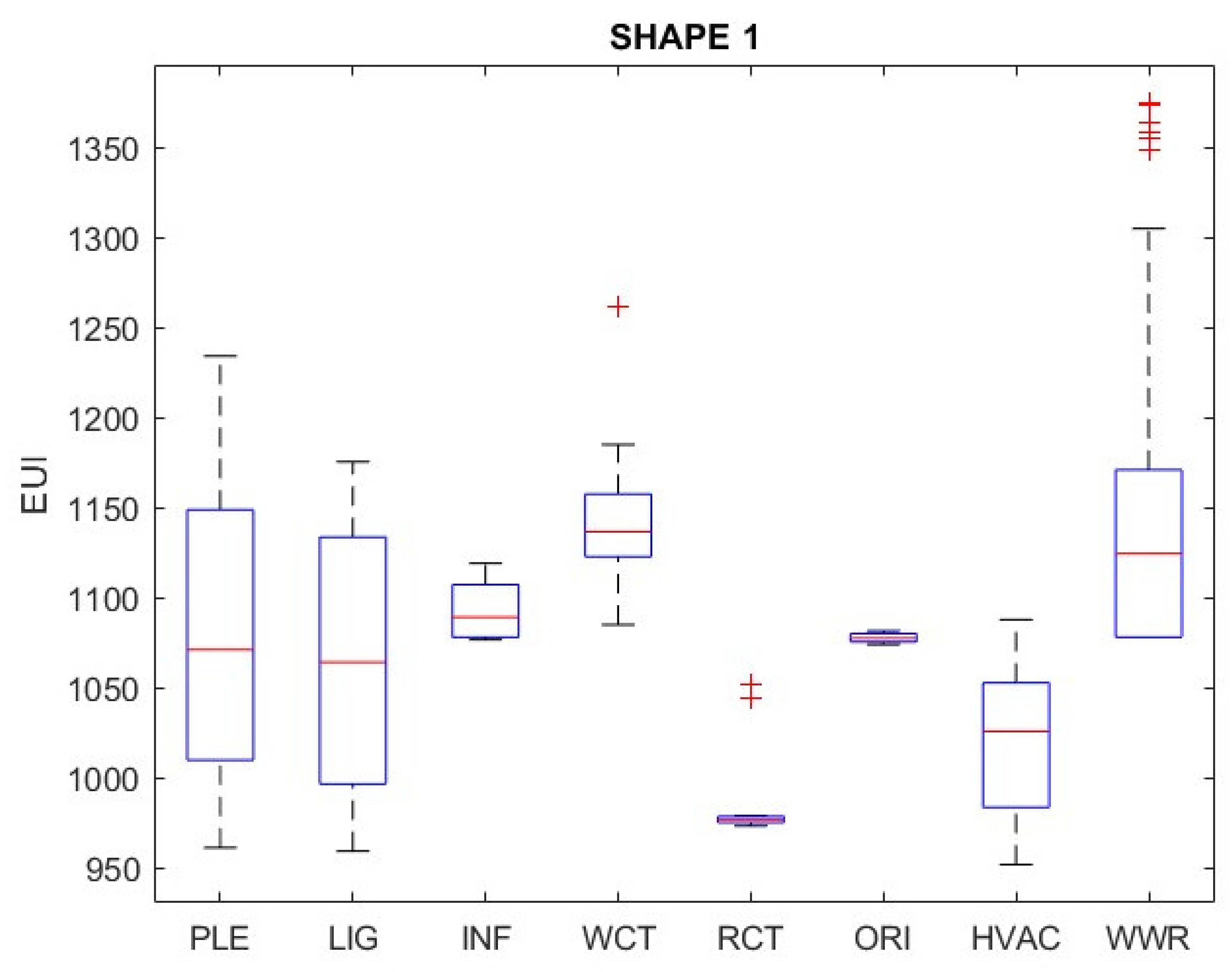
5.2.1. EUI vs. Selected Building Variables

Figure 5 demonstrates the distribution of each design variable directly by using a boxplot.
The data distribution of PLE is observed to be skewed towards the lower side, which is consistent with the trend of the selected values of PLE. Similarly, the EUI values corresponding to LIG are in line with the distribution of the independent variable values, and the data distribution is visually more centered. The whisker for LIG is shorter, which means that the data for LIG are more concentrated than for PLE. The data distribution for INF is significantly lower, with the lower quartile almost coinciding with the lowest quartile and the median skewed towards the lower side. For WCT, the data are skewed towards the low side overall, and there is an outliner; this is because the lower values are more concentrated when the WCT variables are selected, and there is a larger independent variable, which makes the data distribution sparse as the independent variable increases. For the RCT, the graph shows that the data are very concentrated, and there are two outliners, which occur for similar reasons to the outliners in the WCT.
It is worth noting that the WCT and RCT are the main variables determining the building envelope. The distribution of WCT has a larger variation than RCT, which means changing the WCT (wall U-Value) has a greater impact on the EUI. The ORI also has a very concentrated data distribution, with the median in the middle of the box. The HVAC has a skewed high-side distribution with a moderate degree of variation. The WWR has many significant outliers and a high degree of variation, which is considered non-normal.

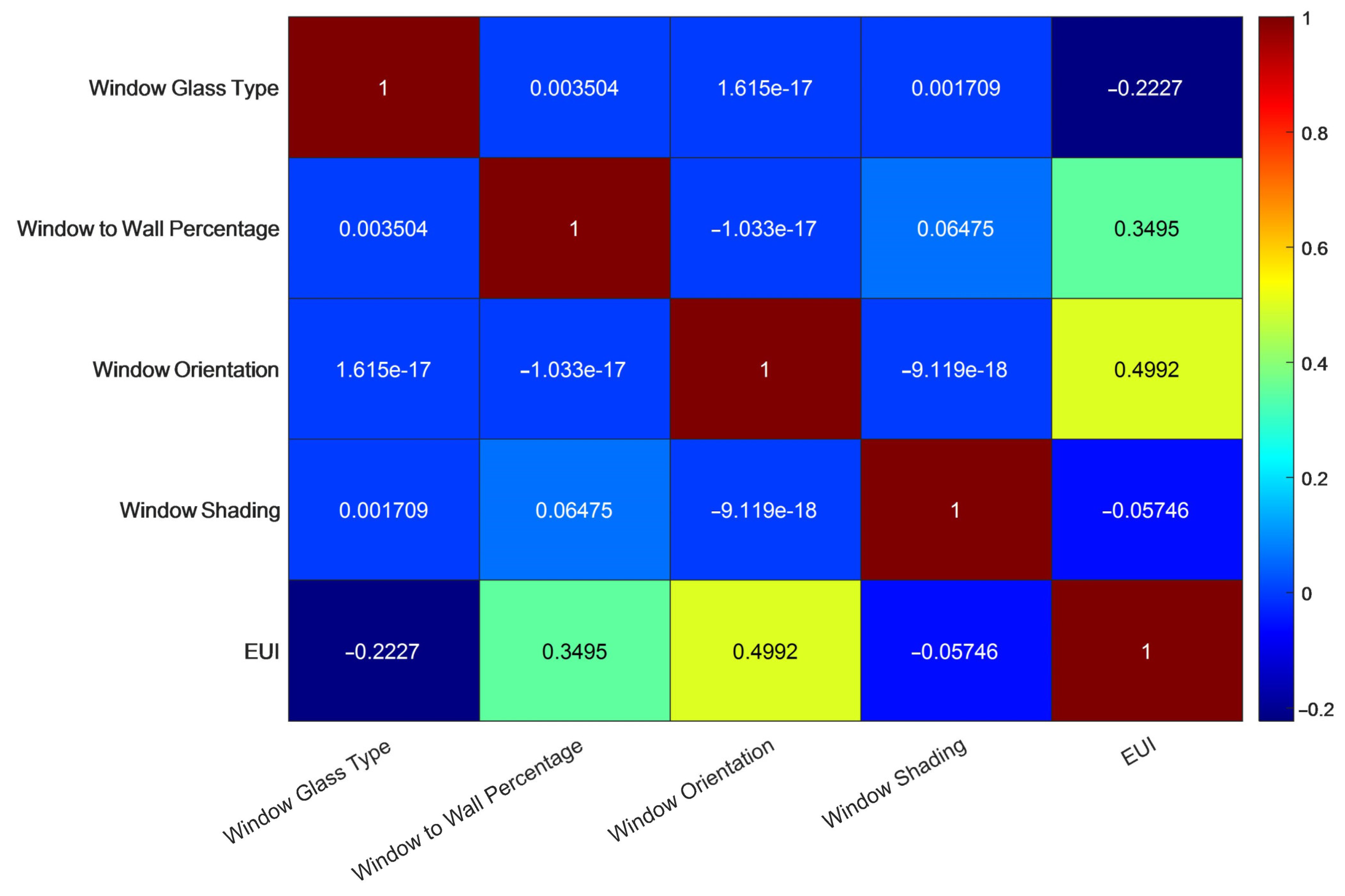
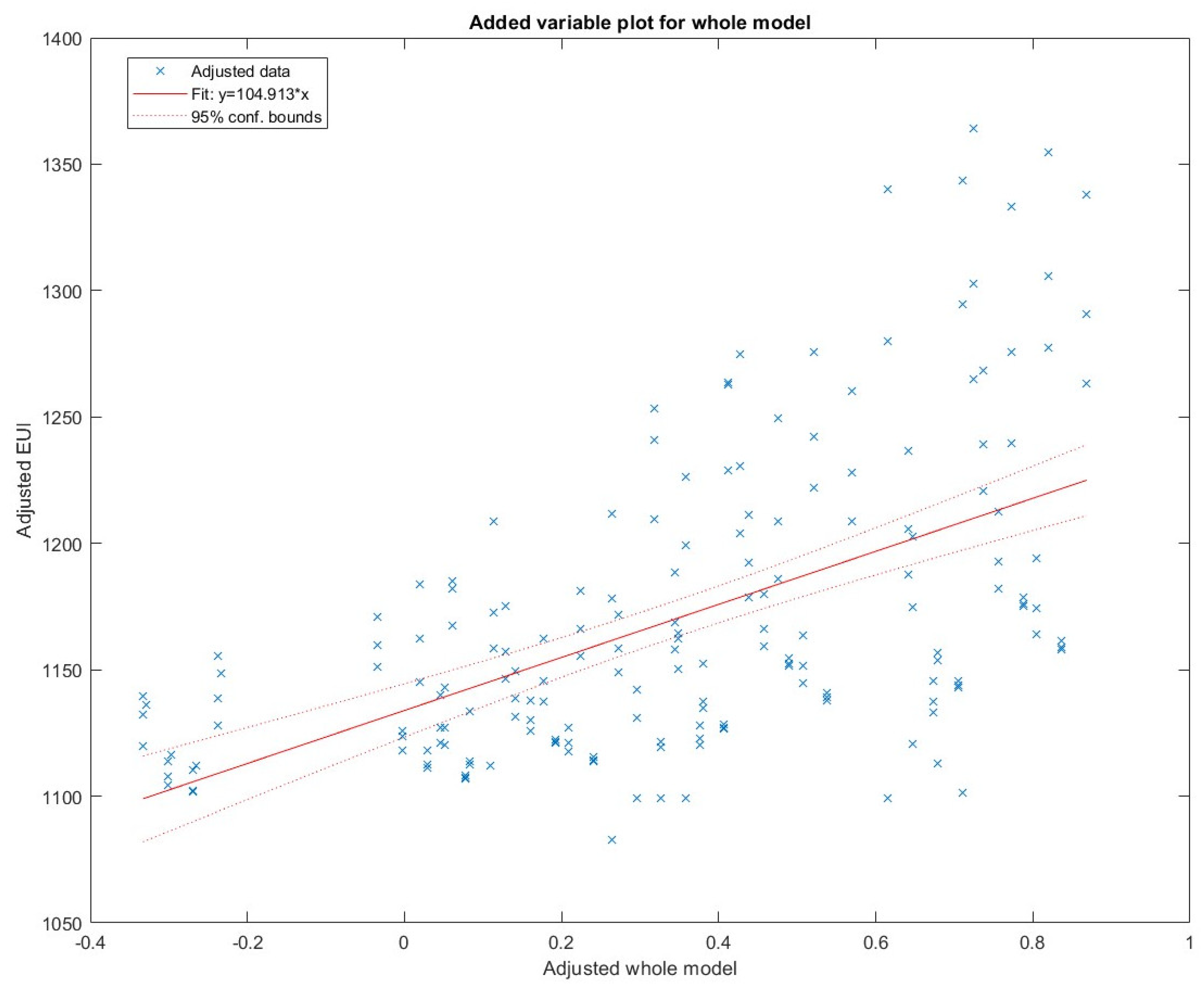
5.2.2. Correlation Analysis for WWR

As mentioned earlier, WWR has several internal influencing elements: window shading, window orientation, window glass type, and window-to-wall ratio. EUI is determined by these elements together, leading this paper to use multiple linear analysis rather than simple linear regression. The outliers and wide variations are considered the results of changing these four elements.
It is noteworthy that window glass type and orientation are categorical variables. Therefore, this paper uses window U-Values and the rotation angle from the north to represent these two variables, respectively. Meanwhile, both window shading and the window-to-wall ratio are percentages. Table 7 shows these elements and their numerical values.
Figure 6 displays the correlation coefficient (r) among WWR internal independent elements and dependent variables, which is EUI. The range of r should be from −1 to 1, while a negative r value represents two variables that have a negative correlation, and a positive r value means two variables have a positive correlation. This paper shows the correlation coefficients among variables from −0.2227 to 1.
According to Figure 6, the correlation between window glass type, window shading, and EUI is negative, which represents that EUI increases with the decreasing window glass type (U-Value) and window shading, while the window-to-wall percentage, building orientation, and EUI have a positive correlation. Additionally, the correlation between window-to-wall percentage and building orientation is considered as strong, while window glass type (U-Value) has a moderate correlation to EUI.
It is also worth noting that window shading has an extremely weak correlation to EUI, which is less than −0.1. Additionally, Table 8 summarizes the change in adjusted R-square when dropping different elements. It can be found that the adjusted R-square only decreases by 0.71% when dropping WS. By considering the above statement, window shading has an extremely weak correlation to EUI and a very limited contribution to the regression model. Therefore, window shading is dropped during the multi-linear regression analysis. For the adjusted R-square, as mentioned in Section 4.3, the EUI is chosen as the dependent variable to represent the building energy consumption. Therefore, the remaining three elements, which are window glass type (U-Value), window-to-wall percentage, and window orientation, are considered the independent variables.
The multi-linear regression model is developed in MATLAB. Table 9 shows the coefficients for three independent variables and intercept values for the equations of seven different shapes. The p-values of each shape are less than 0.05 (5%), which means the significance of the regression model is above 95%, and the model is significant.
According to the multi-linear regression equations listed above, the regression models have a high level of RMSE, and the adjusted R-Square values are low. These indicators represent that the accuracy of models is low. The best-fitted line cannot represent the most data points. Figure 7 also verifies this statement.

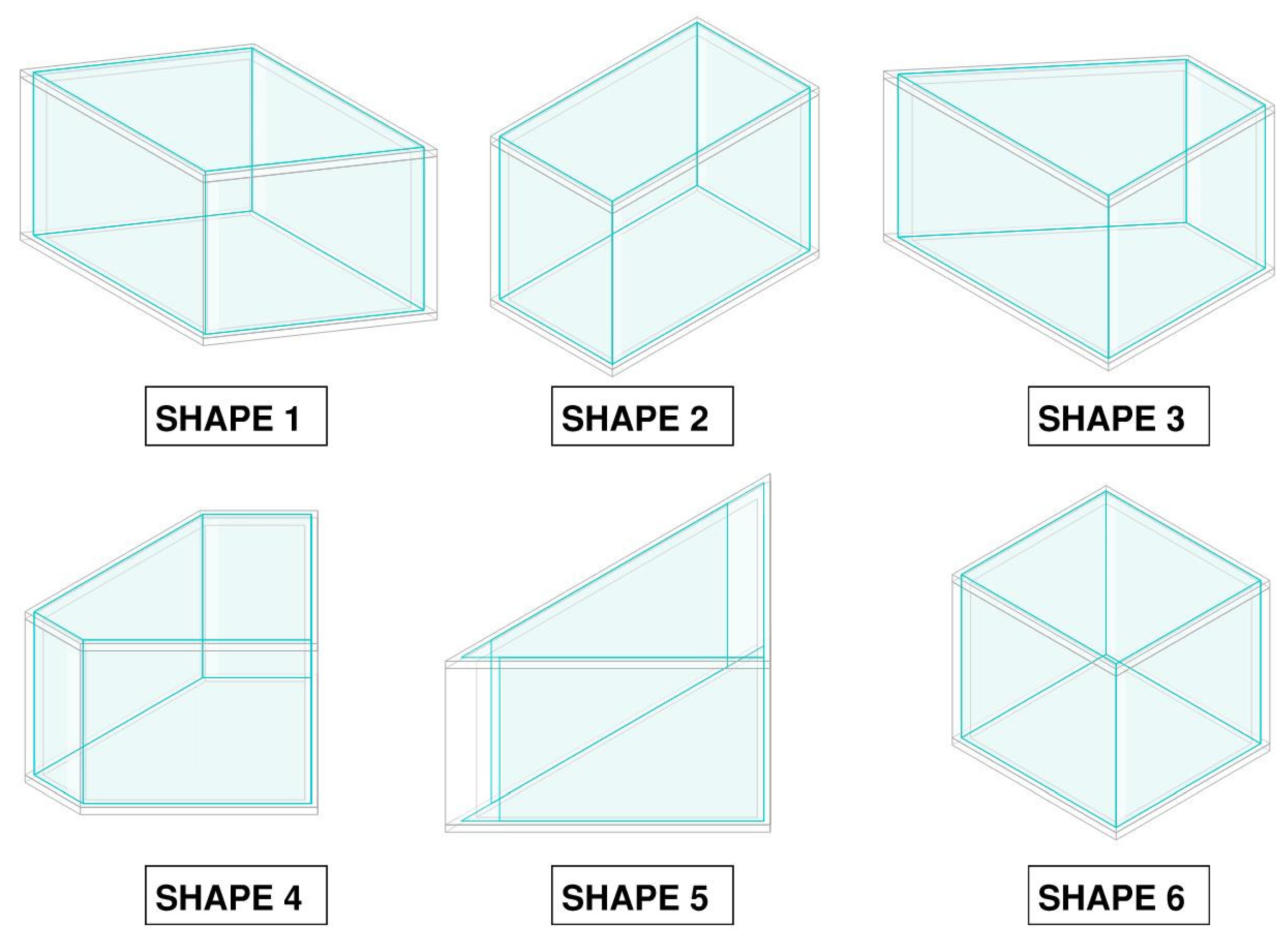
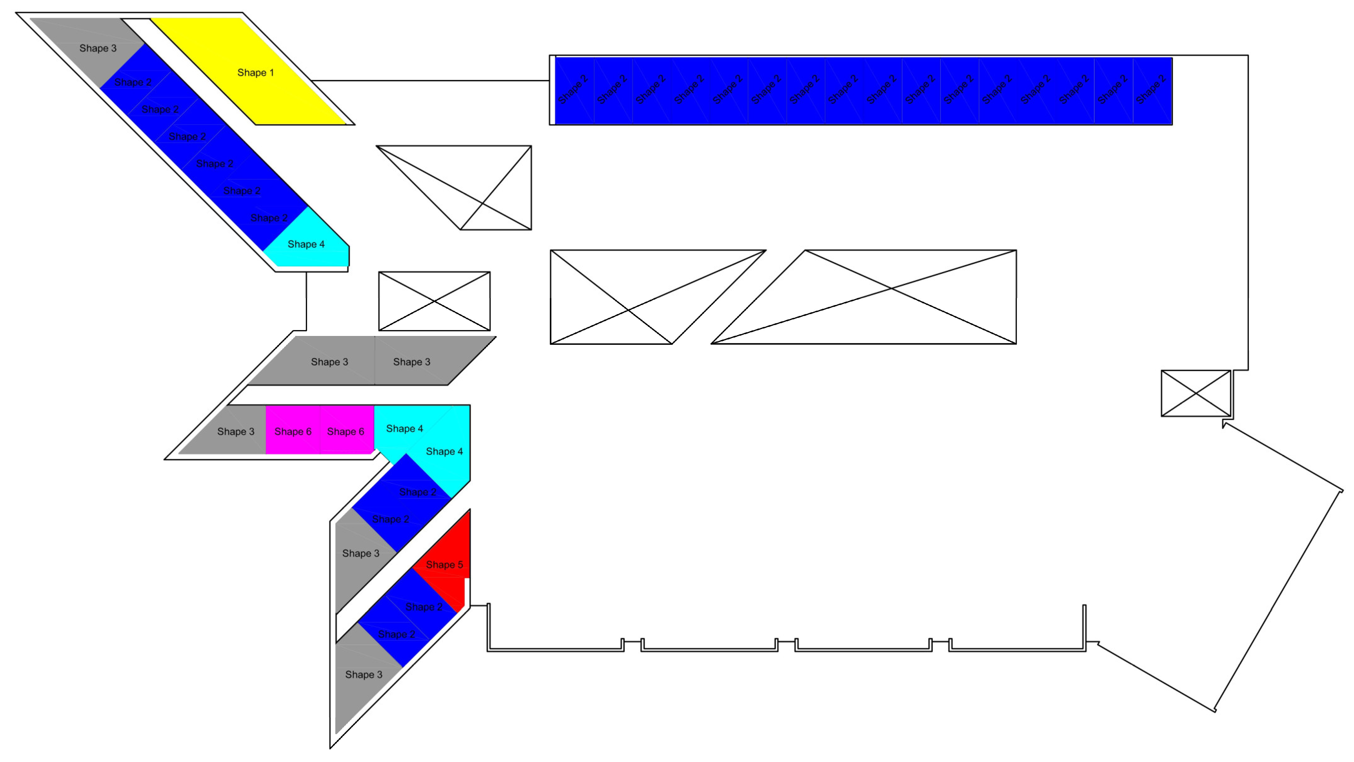
5.2.3. Interactions between Shapes and Building Variables

This part aims to discuss the results of the interaction between building shapes and building variables on EUI.
The effects of changing the wall construction type (U-Value) on EUI are demonstrated in Figure 8. EUI and wall construction type (U-Value) have a positive relationship. It is noted that the EUI increases rapidly when the U-Value is less than 0.5, and the trend becomes gentle when U-Value is higher than 0.5. These trends indicate that changing with a range of U-Value less than 0.5 significantly reduces EUI, and with the increasing in wall U-Value, it has less importance on EUI.
The obvious differences in EUI are observed among the six shapes. Shape 1 has the highest level of EUI value, while Shape 5 has the lowest one. It also shows using wall material with poor thermal insulation has a minor impact on EUI in Shape 5, when the wall U-Value is higher than 0.5.
Figure 9 displays the effect of roof construction type (U-Value) on RUI among different shapes. As demonstrated in the figure, EUI has a positive relationship with roof U-Value. EUI increases steeply when the roof U-Value is less than 0.5, and the slope increases slightly when U-Value is higher than 0.5. These trends also indicate that controlling EUI by changing the roof U-Value is less effective when the U-Value is higher than 0.5.
According to Figure 9, Shape 2 has the highest value of EUI among all roof U-Values, while Shape 5 has the lowest one.
The trends of EUI vs. infiltration rate are displayed in Figure 10. The infiltration rate and EUI are correlated positively. Generally, the slope is considered steady. The trends of all shapes show common linear relations with positive trends.
The figure also shows Shape 2 has the highest level of EUI in all infiltration types, while Shape 5 has the significantly lowest one.
Figure 11 demonstrates the trends between lighting efficiency and EUI among different shapes. The lighting efficiency has positive trends with EUI, and the trends are considered general linear relations for all shapes as all slopes are steady.
Shape 2 has the highest level of EUI, while Shape 5 has the lowest one. Moreover, the difference in EUI is not significant among all shapes except five, as the lines of these five shapes are close to each other.
The relationships between EUI and plug load efficiency for different shapes are demonstrated in Figure 12. Similar to trends in lighting efficiency, plug load efficiency has a positive linear relationship with EUI, and different building shapes have minor effects on EUI except Shape 5.
To summarize the figures in Section 5.2.3, Shape 1 has the highest EUI of WCT, and Shape 2 has the highest EUI of all other variables. Shape 5 has the lowest EUI of all variables. This means Shape 5 is the most energy-saving one among all shapes. No significant difference in EUI of different shapes is observed, except in Shape 5.

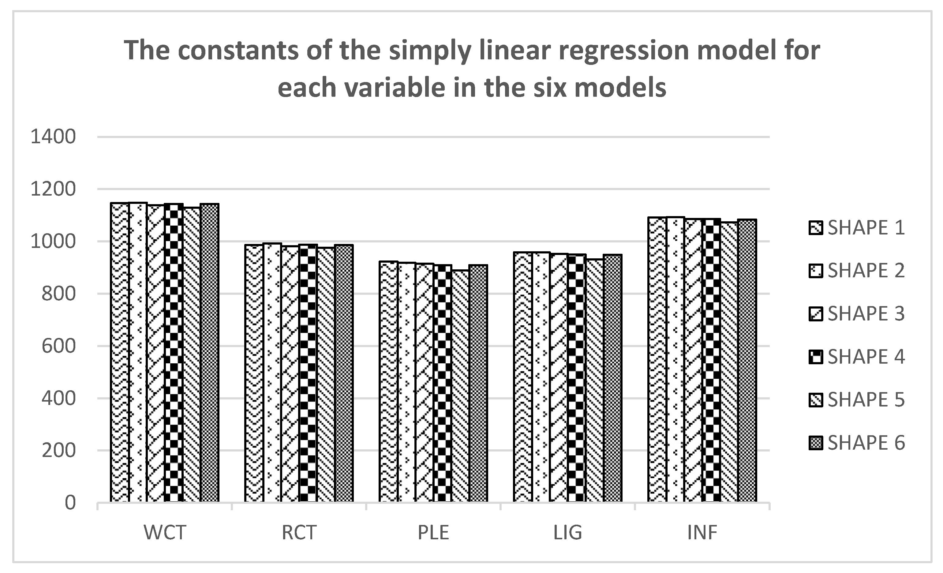
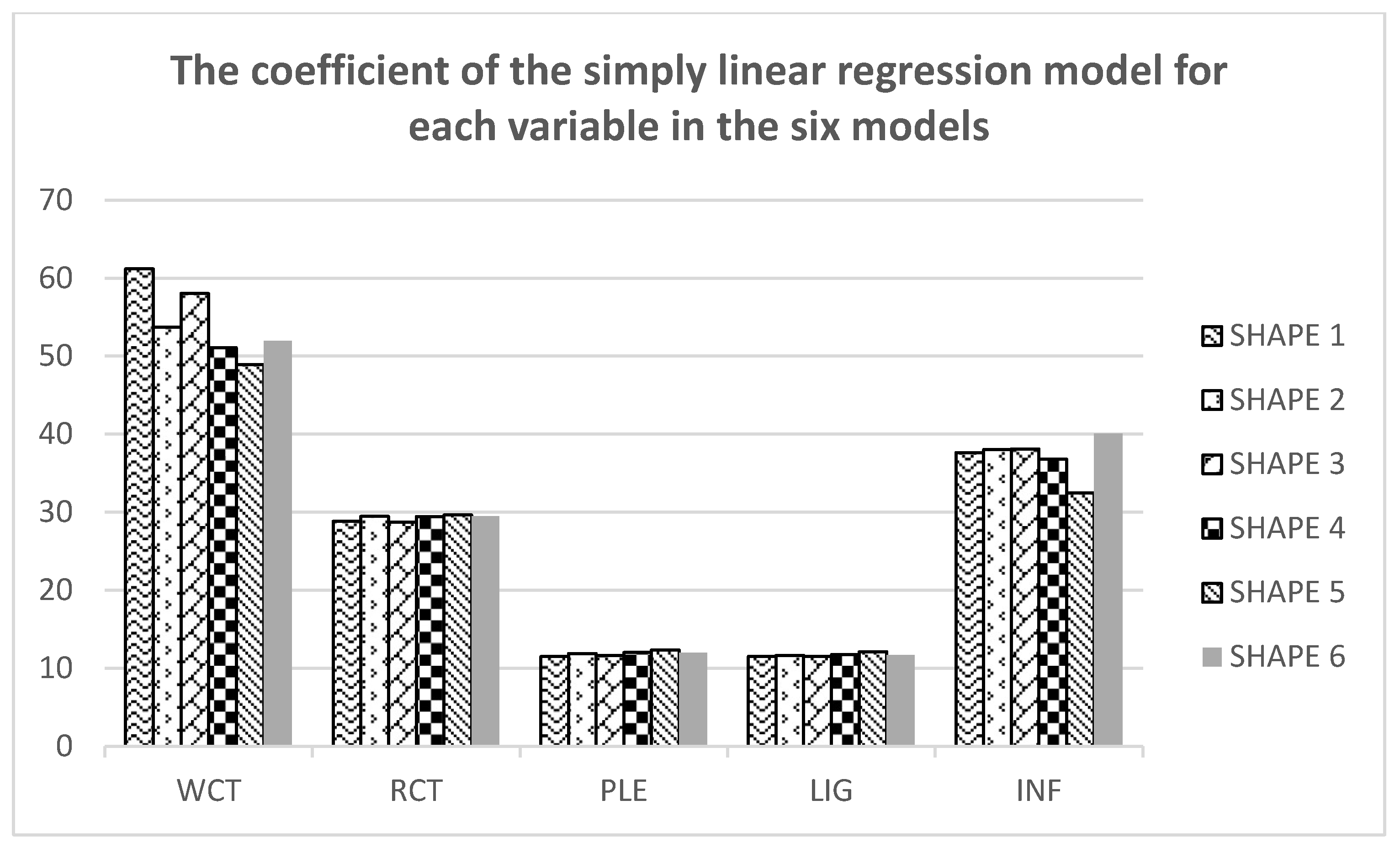
5.3. Simply Linear Regression

The results of linear regression analysis are displayed and illustrated in the following content. The best-fit lines are generated. The correlation and significance are also discussed. The best-fitted line and 95% confidence bounds/intervals, root mean square error (RMSE), as well as adjusted R-square, are provided to help explain the results.

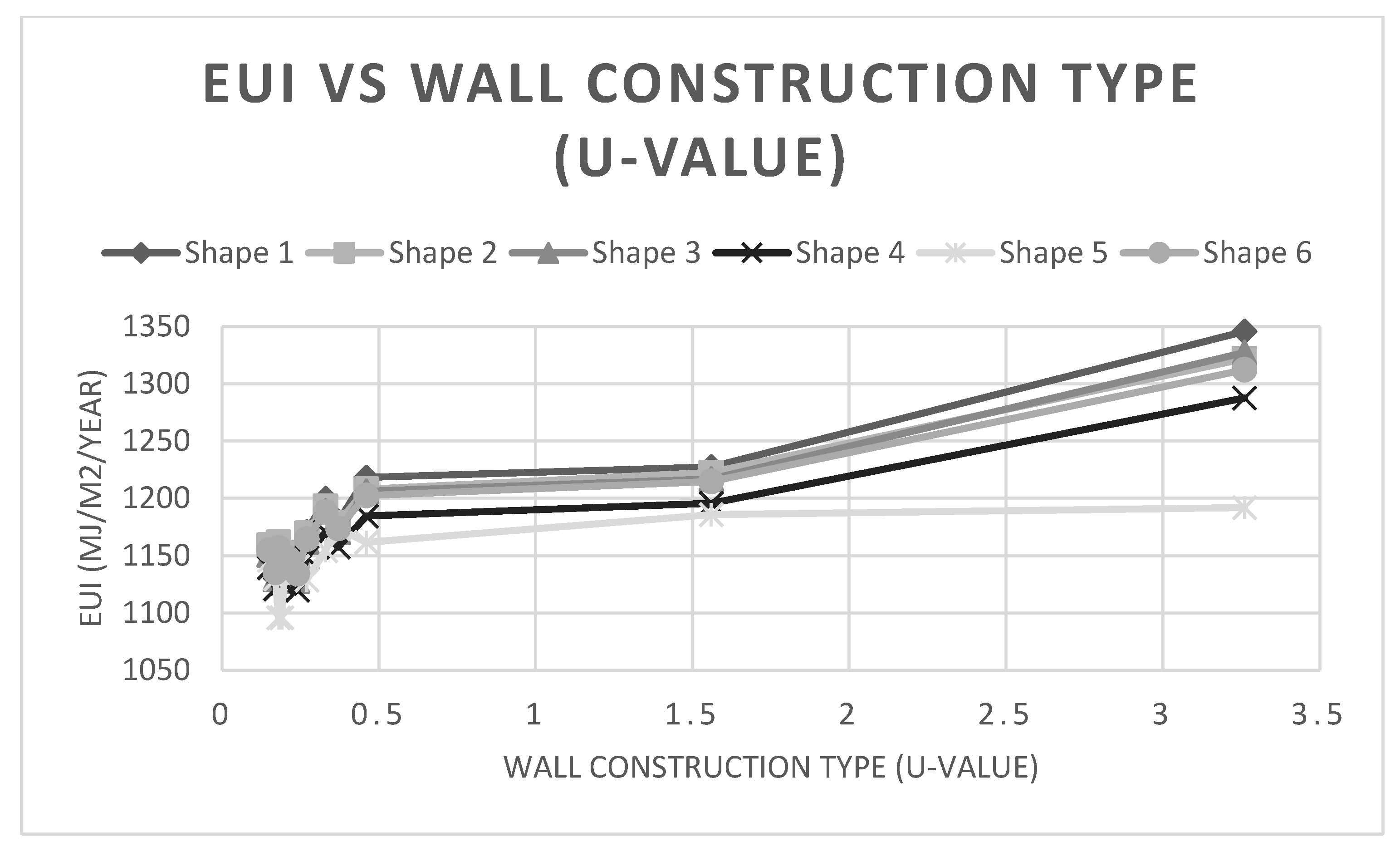
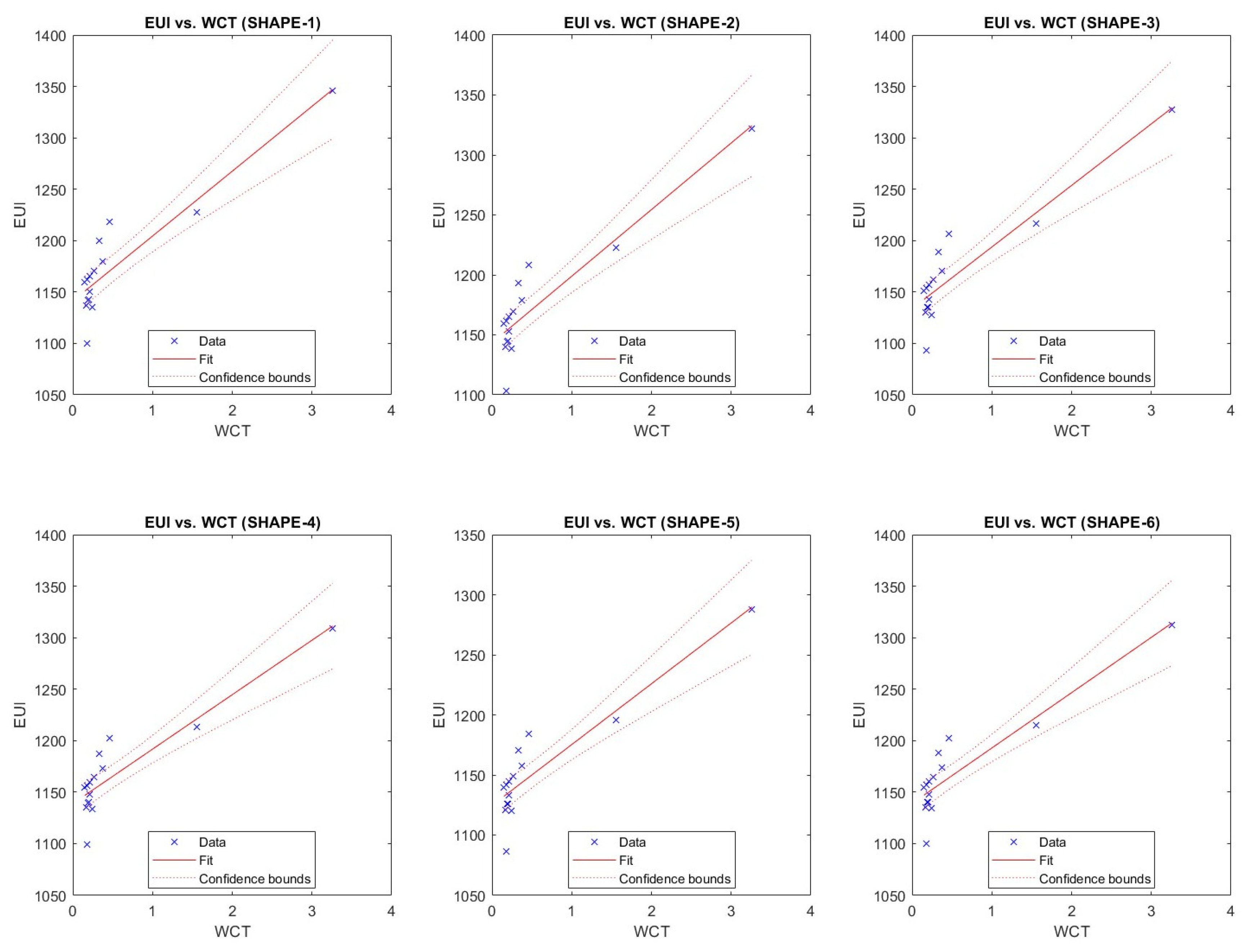
5.3.1. Wall Construction Type

From Figure 13, the relationship between WCT about EUI has the same trends in all six shapes, and they are positively correlated. EUI value increases with the value of WCT rising. The best-fit lines are also shown for six cases, and their equations are listed in Table 10.
As can be seen from the table, the p-values for all six cases are small, which means that the six cases have high significance for the fitness equation. The RMSE is low for all six cases, with Shape 5 having the smallest RMSE, which means that Shape 5 has the least dispersion of observations relative to the fit line. The adjusted R-squared is close to 0.80 for all six cases, which means that the fitted equations can explain 80% of the variation in the observations, which represents a good fit.
Further, Figure 13 also shows the 95% confidence interval for the data, and they are shown as dashed lines. The confidence intervals for the six cases follow the same trend and are narrower where the sample is dense and wider where the sample is sparse. This means that denser sampling reduces the distribution error of the data and thus improves the accuracy of the data. As GBS only offers a limited selection of WCTs, it leads to uneven sampling in the range of WCT values greater than 1.0. This results in wider confidence intervals and higher errors between the observed and true values of the objects.

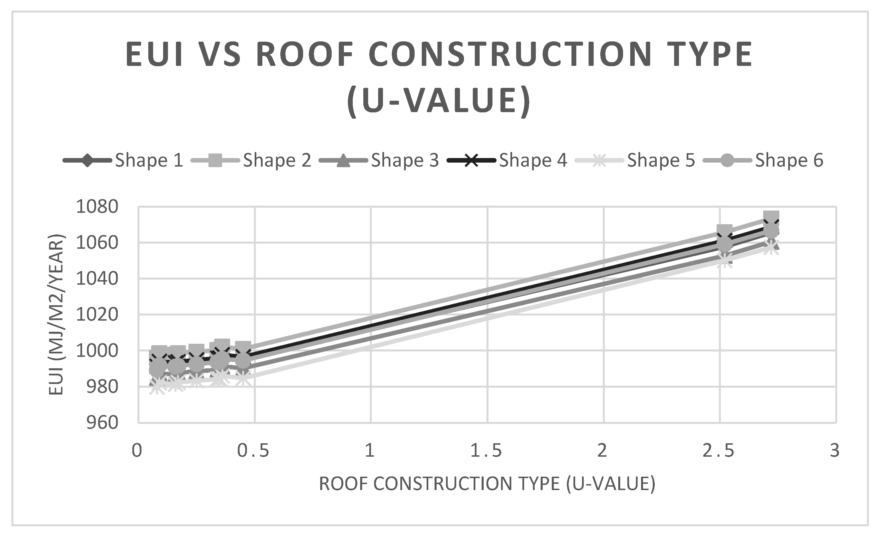
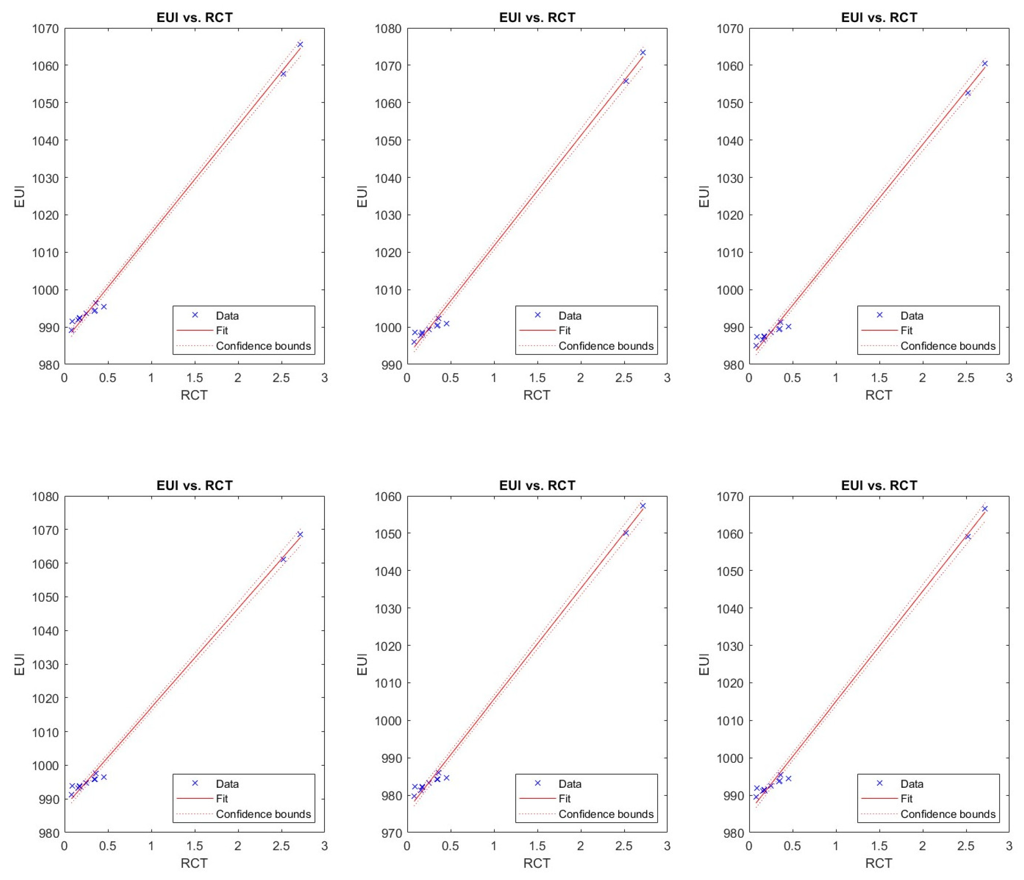
5.3.2. Roof Construction Type

As can be seen from Table 11, the p-values for all six cases are much smaller than that of WCT, which means that the six cases have extremely high significance for the fitness equation. The RMSE is low for all six cases, with Shape 1 having the smallest RMSE, which means that Shape 1 has the least dispersion of observations relative to the fit line. The adjusted R-squared is close to 1.000 for all six cases, which means that the fitted equations can explain most of the variations in the observations. The results represent the observations are almost identical to the regression model, with positively linear correlations.
Additionally, similar to the WCT, the sampling data for the RCT is sparse in intervals greater than 0.5. Interestingly, it can be observed from the Figure 14 that the confidence interval for the RCT, even though gradually widening, remains relatively narrow when the RCT equals around 2.5 since the last two sample value lines of the RCT are closer than those in WCT, which characterizes the above statement that the larger the sample size, the narrower the confidence interval and the observations are more representative of the true values.

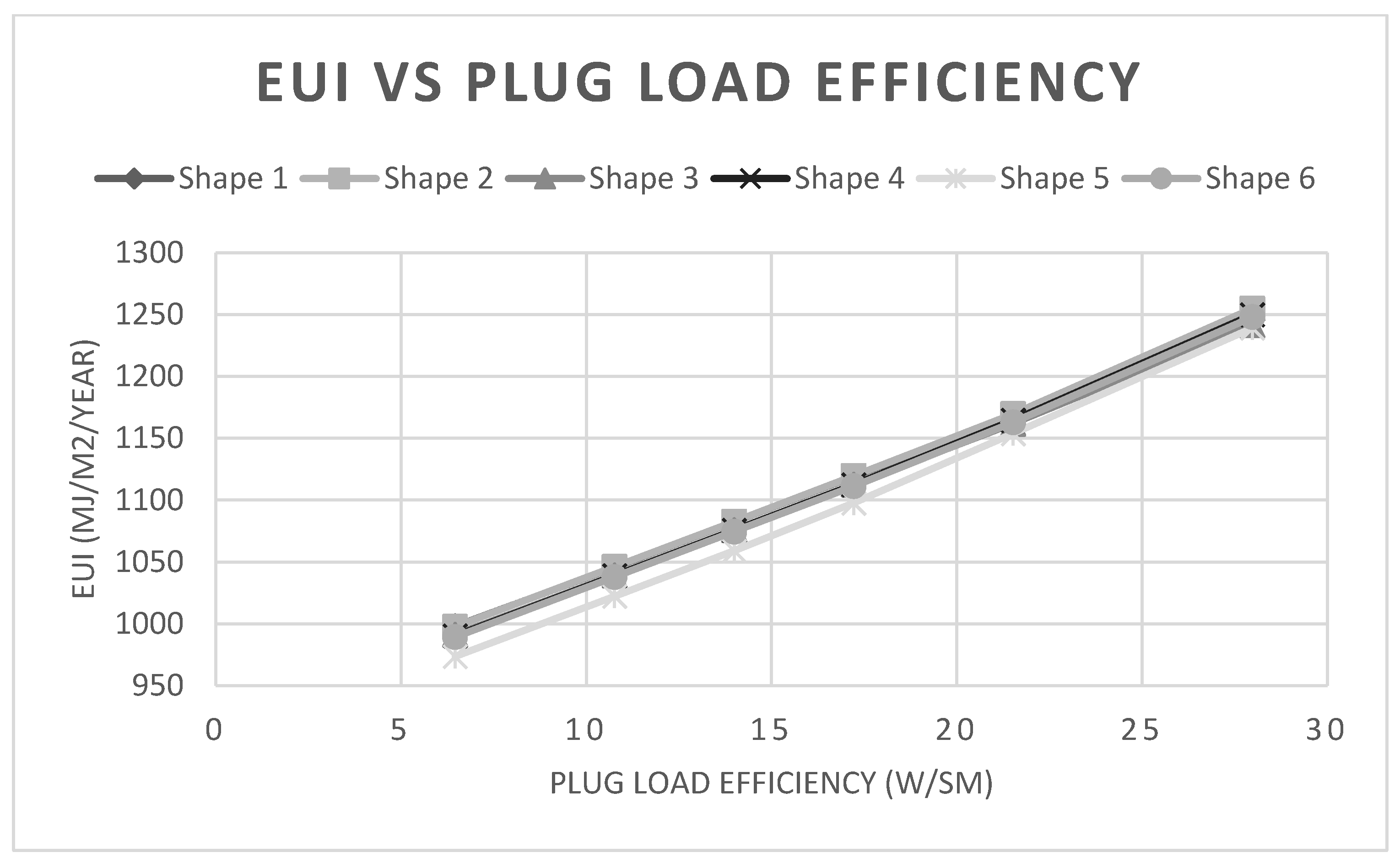
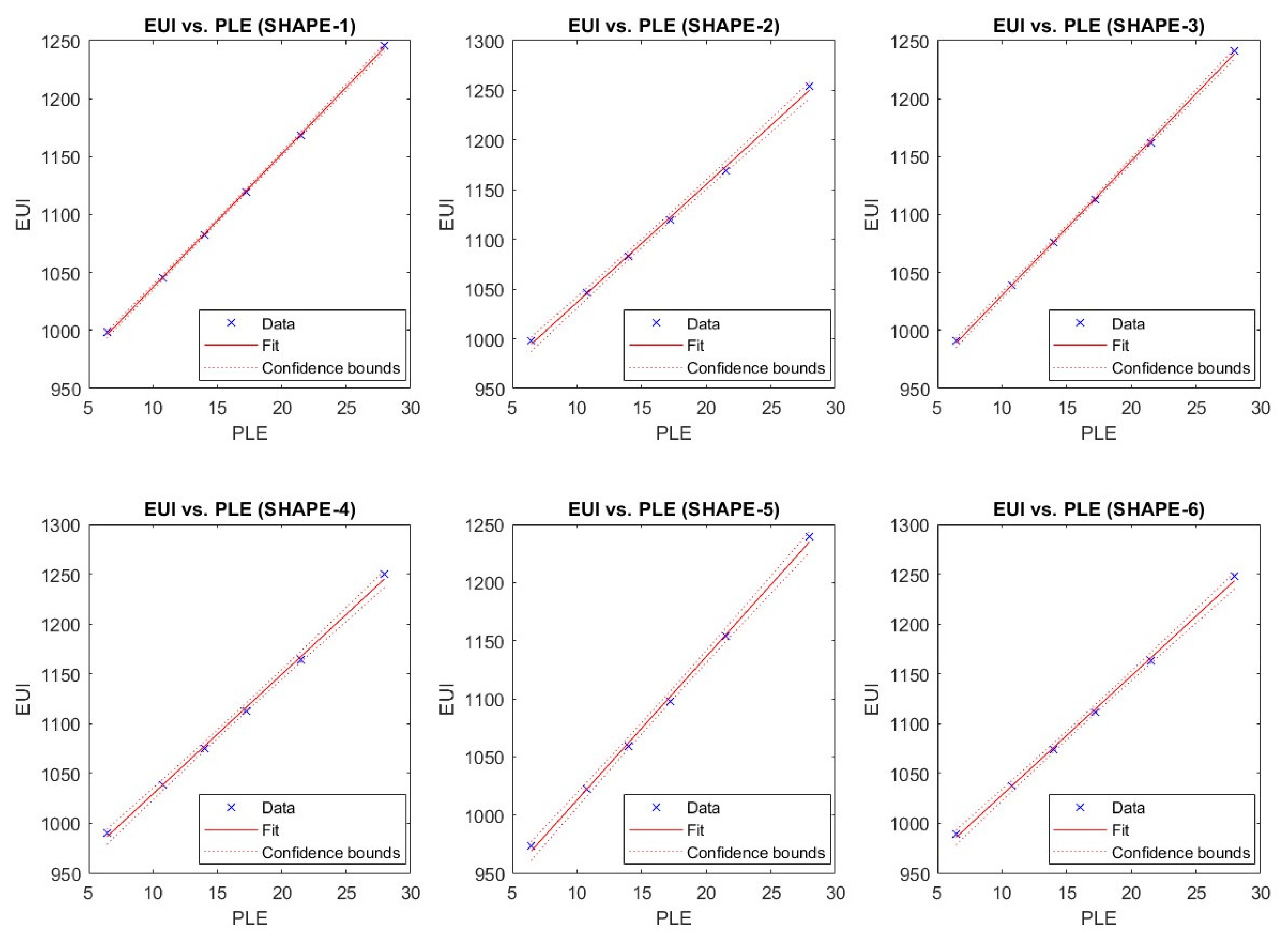
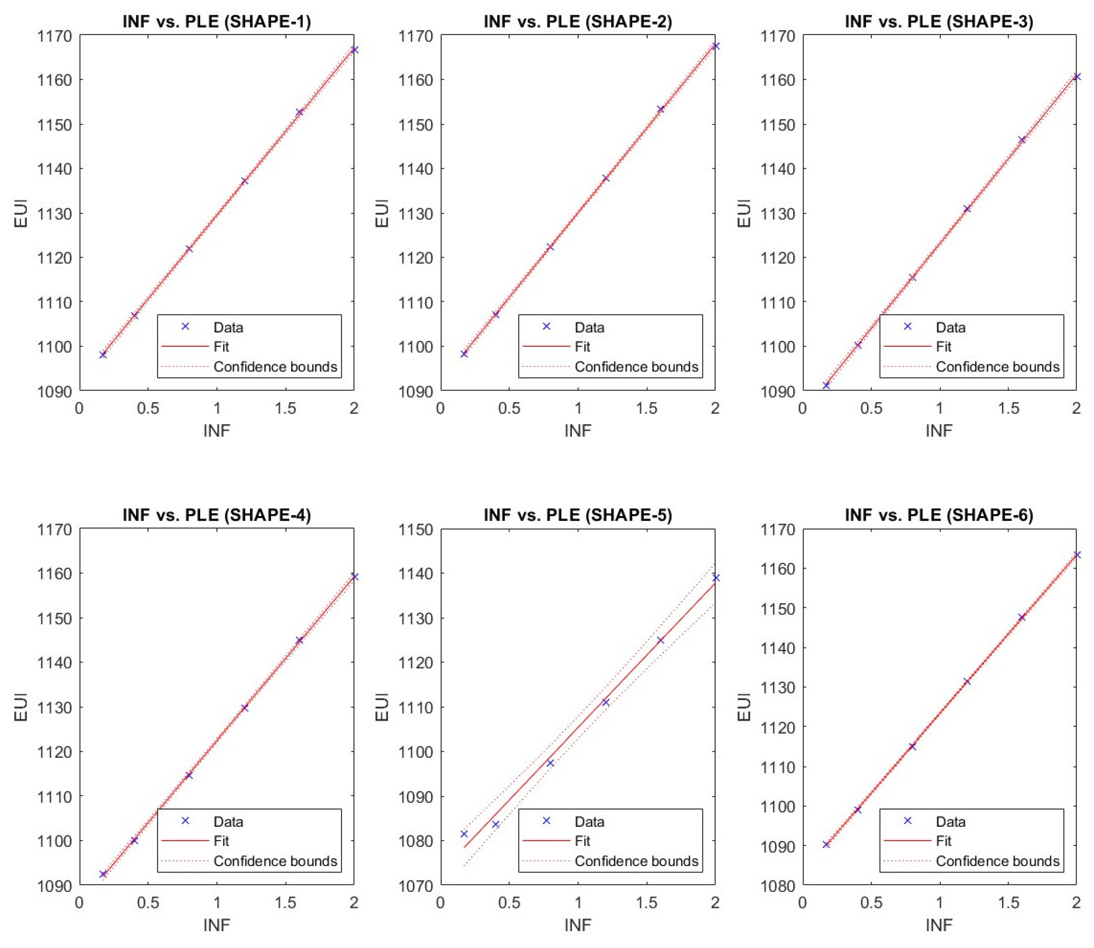
5.3.3. Plug Load Efficiency

Figure 15 demonstrates the trends in PLE and EUI among six shapes. The EUI is positively correlated with the PLE, and the six shapes of the PLE adaptation lines are in general agreement with the observed data. The more evenly sampled values and the fact that one value was taken for each 0.4 resulted in a more consistent confidence interval, and the wider ends shown in WCT and RCT do not appear here.
Table 12 shows the fit line equations and the results of statistical indices. Comparing the magnitude of the fit line coefficients, it can be concluded that the PLE has a more significant effect on the EUI in Shape 5. The regression models on all six shapes have very small RMSE and p-values, which means that the values predicted by the regression models have very small errors compared with the observed values and that the regression models are highly significant. It is worth noting that the adjusted R-squared values are consistent, and the value of Shape 1 is equal to 1, which means that the regression model explains all the observed variations completely and that there is a certain positive linear relationship exists between these two variables.

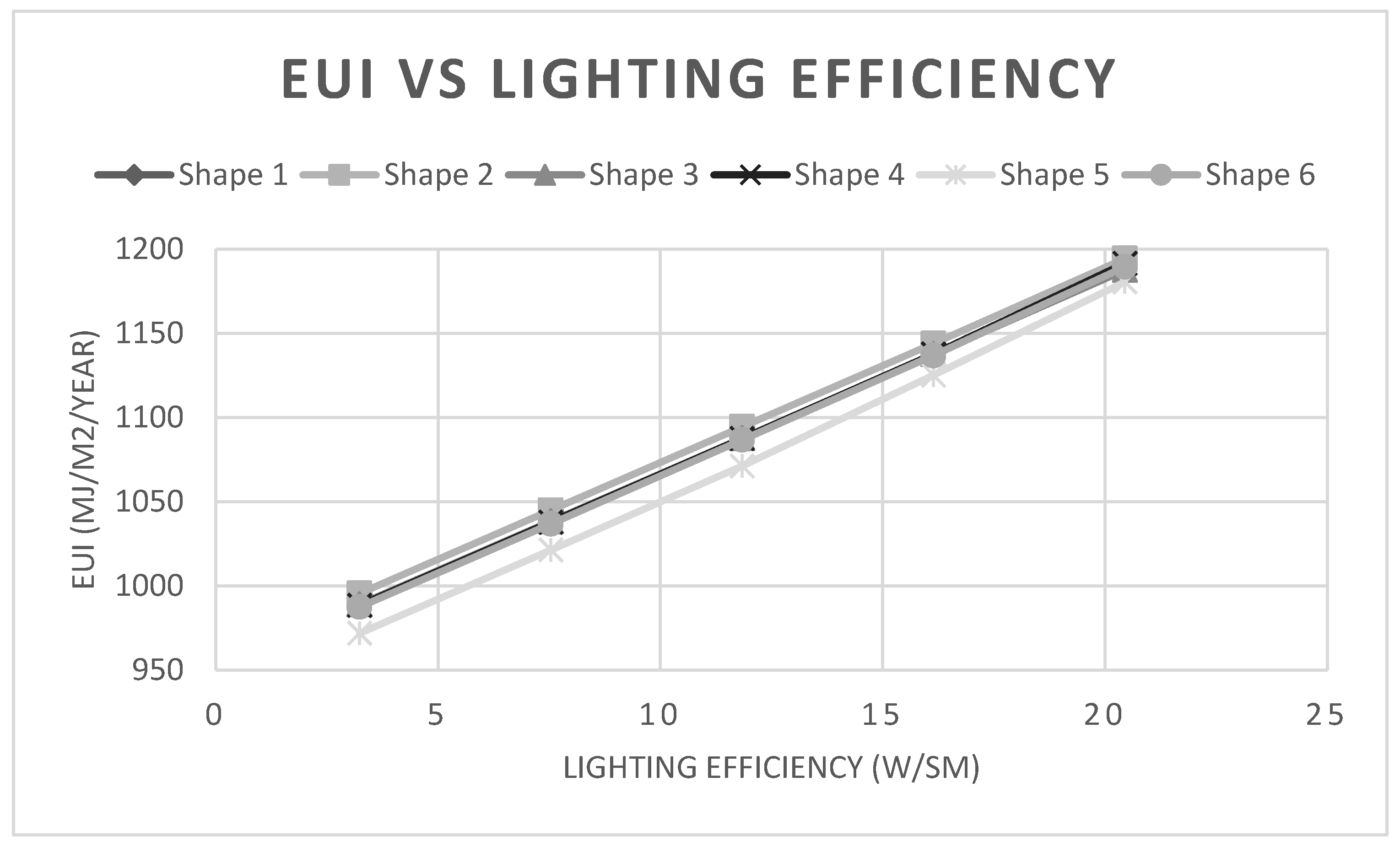
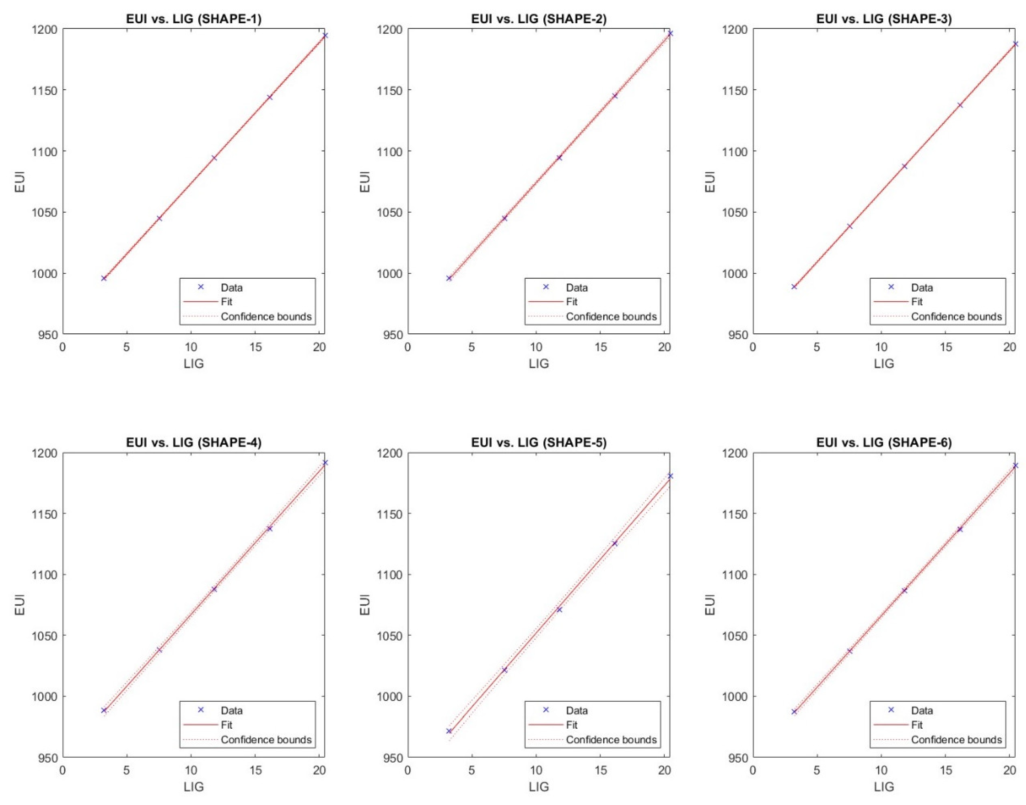
5.3.4. Lighting Efficiency

The trends of EUI about LIG are shown in Figure 16. Similar to the PLE, the observations of the LIG are almost in a straight line, and the regression model is close to the observations. The uniform sampling allows for a narrow range of confidence intervals and small errors in the observations relative to the true values.
Table 13 shows that the effect of LIG on EUI is greatest for Shape 1, with small RMSE and p-values for all six shapes, meaning that the observations are evenly distributed, and the null hypothesis is less likely to be true, the null hypothesis can be rejected, and the regression model results are significant. Five of the six models have an adjusted R-squared equal to 1, which means that the observations are perfectly explained by the regression model and that LIG is positive and linearly associated with EUI.

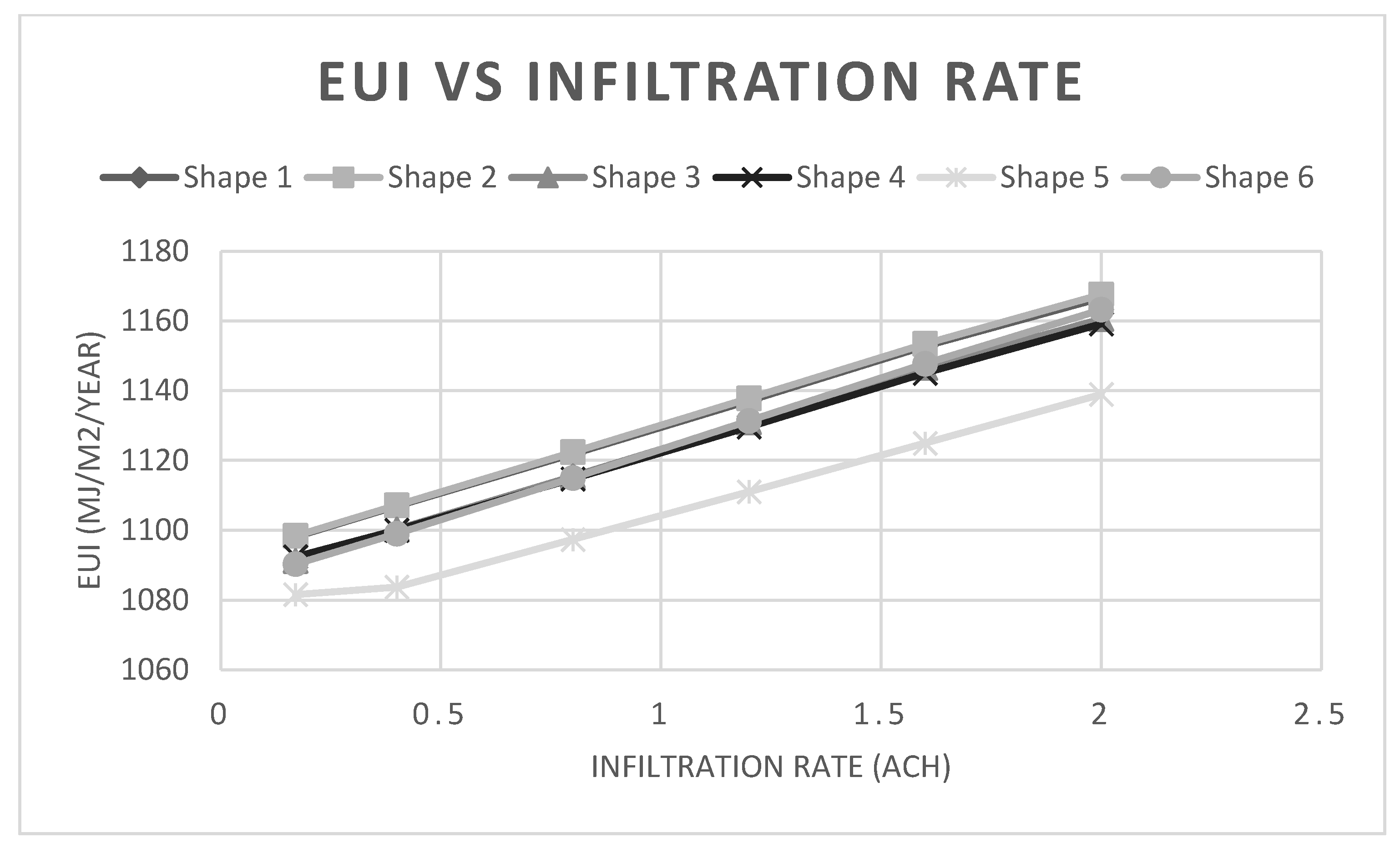
5.3.5. Infiltration Rate

The trends of EUI about INF are shown in Figure 17. The observations of the INF are almost in a straight line, and the regression model is close to the observations. The uniform sampling allows for a narrow range of confidence intervals and extremely small errors in the observations relative to the true values. However, in Shape 5, the confidence interval is larger at the beginning (in the range of 0.0 to 0.5) because the observed values are not distributed linearly. The different slopes resulting from the non-uniform distribution of the first point and the remaining make the confidence interval larger, which demonstrates that there is some error between the observed and true values.
Table 14 shows that the effect of INF on EUI is greatest for Shape 6, with small RMSE and p-values for all six shapes, meaning that the observations are evenly distributed, and the null hypothesis is less likely to be true, the null hypothesis can be rejected, and the regression model results are significant. Five of the six models have an adjusted R-squared equal to 1, which means that the regression model perfectly explains the observations and that LIG is positive and linearly associated with EUI. Only Shape 5 has a smaller adjusted R-square and higher RMSE due to the anomalies in observed values.
In summary, the RCT, PLE, LIG, and INF regression models fit the observed values well; the observed values have a small margin of error and can reflect the true value well. It is worth mentioning that WCT has a large confidence interval due to the uneven distribution of the sample values, leading to a large error with the true values. The regression model does not fit the observations very well compared with other models. However, WCT has a relatively high level of adjusted R-square; these minor dispersions of the observed values are attributed to a reasonable and acceptable range.

5.4. Parametric Analysis

Figure 18 and Figure 19 demonstrate a comparison of the constants and coefficients of the regression models for all variables selected to perform a simple linear regression analysis for all six shapes. The effect of changing each variable on EUI is presented intuitively in the following content.
The parameter terms for each of the six shape variables are shown in Figure 18, with WCT and INF having the most significant constant terms, followed by RCT, LIG, and PLE. The larger the constant term, the larger the base of energy consumption and the higher the lower limit of consumption. According to the image, the constant terms of the regression models are close to each other. It is worth noting that Shape 1 has relatively high constant terms for PLE, LIG, and INF, and Shape 6 has higher constant terms for the WCT and ECT variables.
Figure 19 shows the coefficients for each variable of the six shape regression models. The coefficients in a regression model determine the degree of influence of that independent variable on the dependent variable, with larger absolute values representing the greater importance of that independent variable on the dependent variable. According to the images, WCT has the most significant coefficient, and WCT has the most effect on energy consumption, followed by INF and RCT. PLE and LIG have similar-sized coefficients and have the least effect on the dependent variable. Shape 1 has the largest coefficient in WCT, which means that changing WCT in Shape 1 has the largest influence on EUI. Conversely, Shape 1 has a non-significant effect on the other variables. RCT, PLE, LIG, and INF have a relatively significant effect on EUI in Shape 6. The RCT, PLE, and LIG have a relatively equivalent effect on EUI.

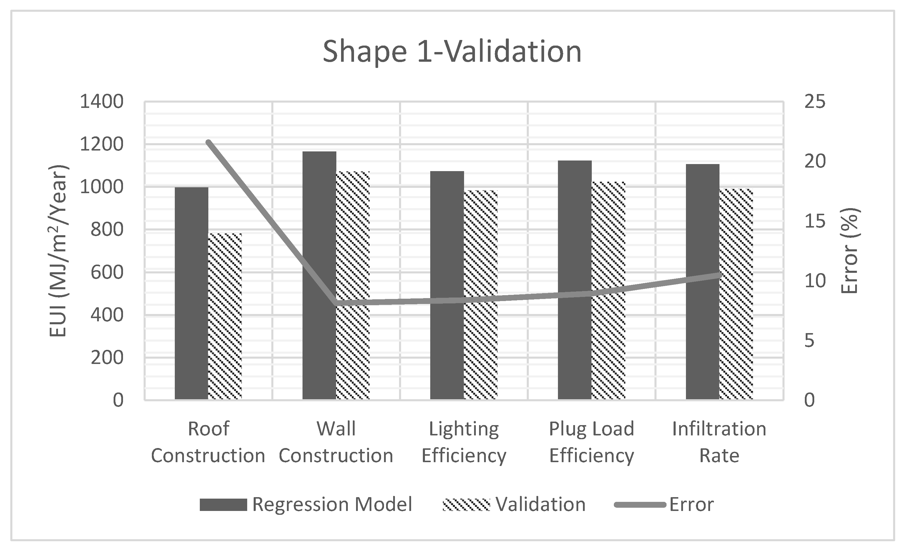
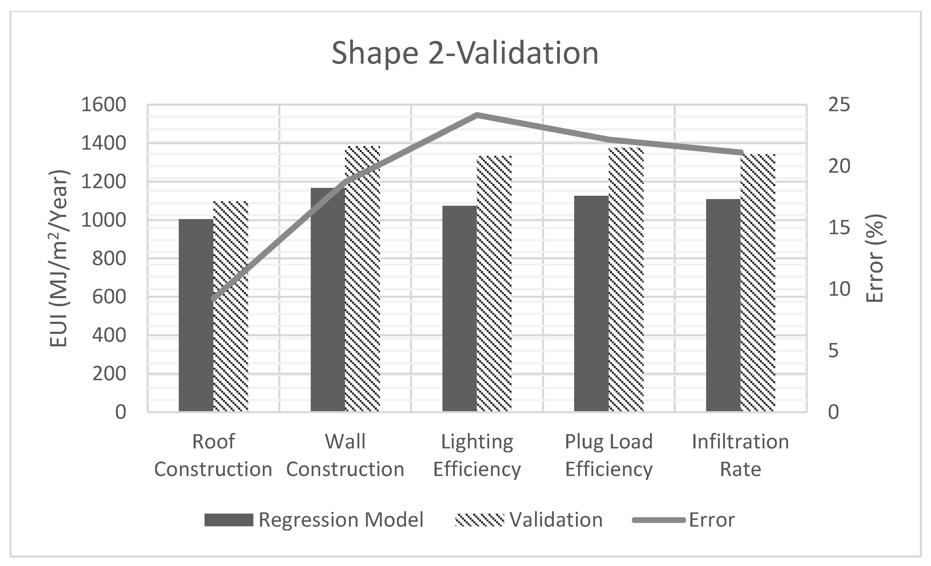
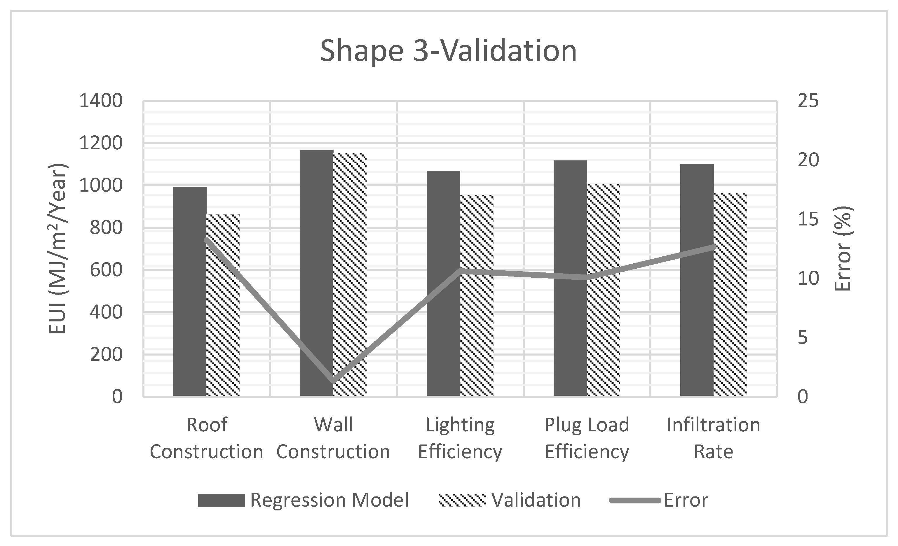
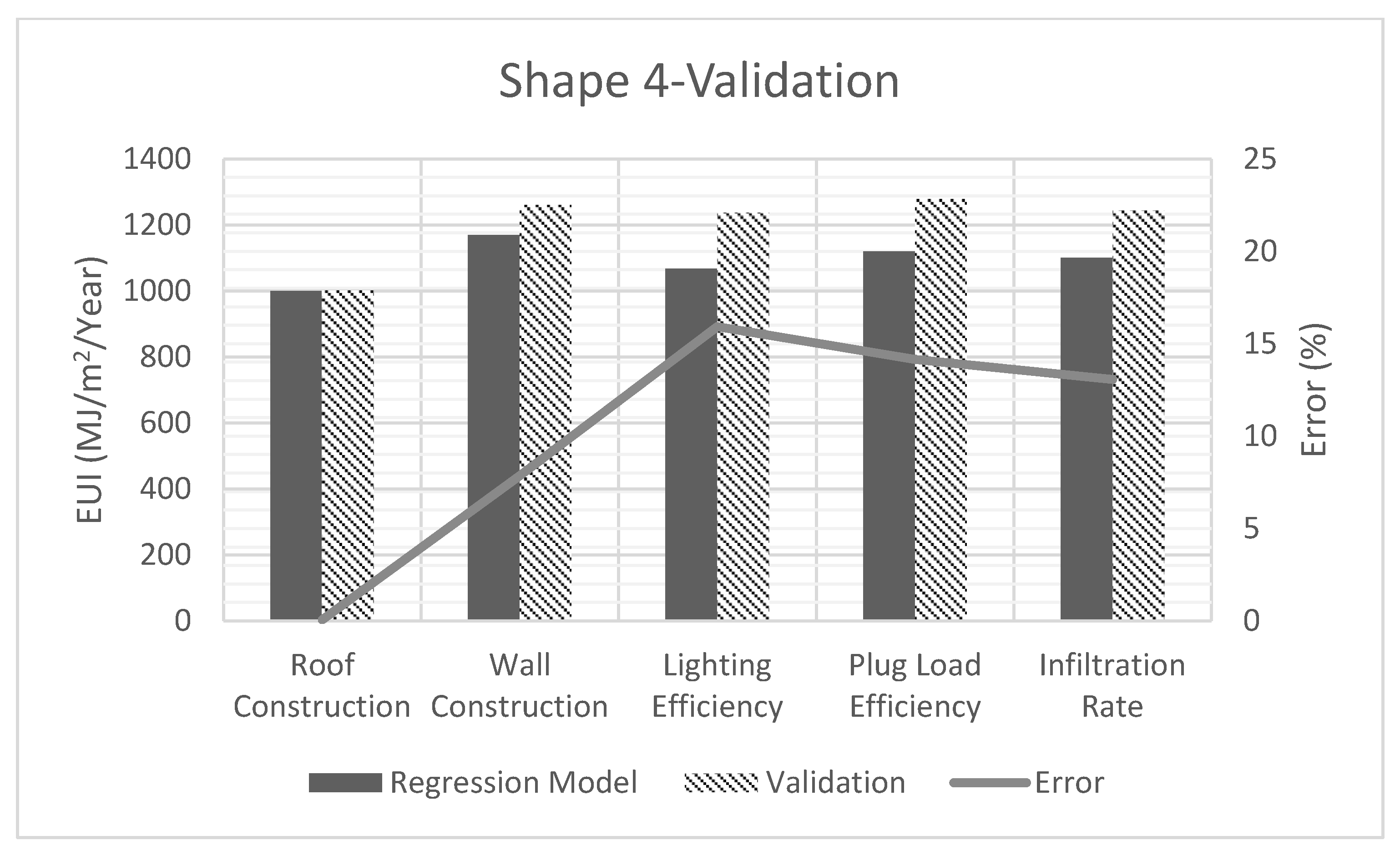
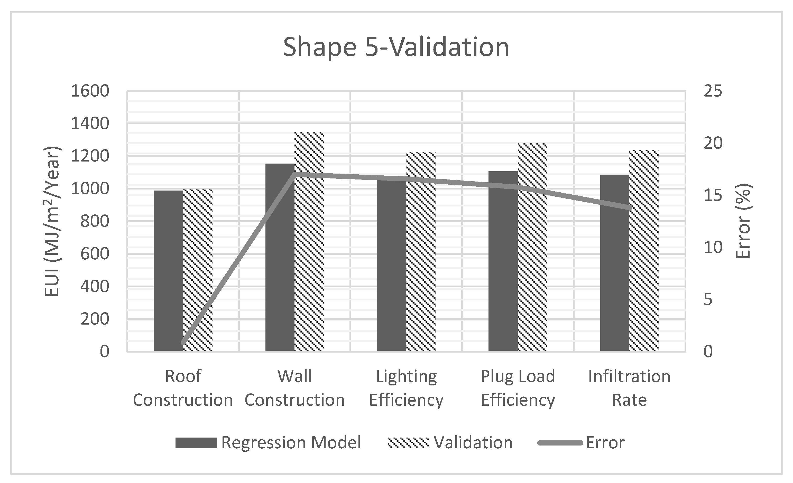
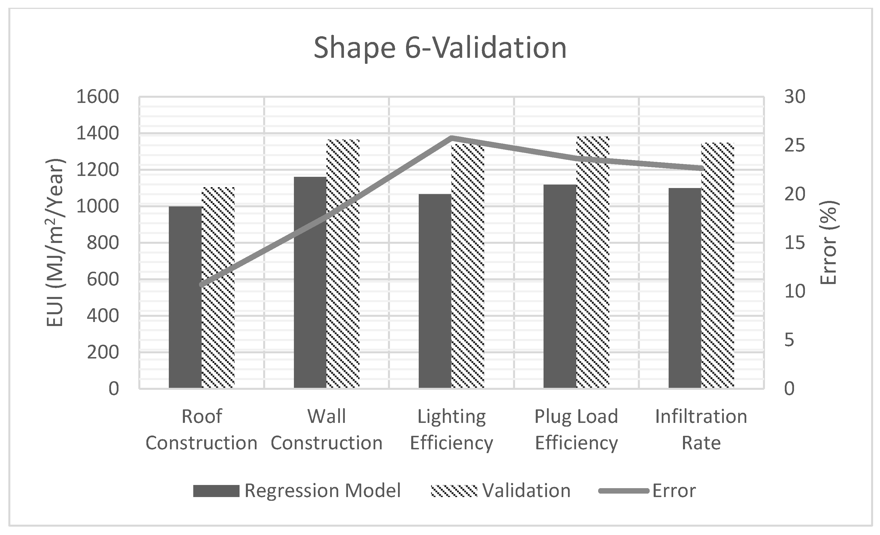
5.5. Validation and Error

The regression model obtained in the previous steps needs to be compared with real TETB office rooms to validate the regression models. Six validation models were built based on real word dimensions, and material properties were all referenced from papers related to TETB or similar projects and standards. Table 15 lists the real and assumed material information of validations.
The following diagrams compare regression models and the models built based on real dimensions. Errors are shown as absolute percentages (Figure 20, Figure 21, Figure 22, Figure 23, Figure 24 and Figure 25).
The above figures show the comparison between the regression models and validation models. The error indicates the accuracy of the regression equations. The maximum error was observed at the lighting efficiency of Shape 6, while minor errors were found in the roof construction of Shapes 2 and 4.
It is worth noting that TETB has several office shapes with sharp angles. There were some gaps between two wall connections with the default analytical space and surface resolution because Revit ignored building components smaller than the resolution.
Generally, the error ranges between 10% and 25%, which is not an acceptable range. The regression equations do not pass the validation process. Hence, the accuracy of the regression models is low. The possible reasons and limitations are discussed below.

6. Conclusions, Recommendations, and Future Research

This study investigates the impact of essential building variables on energy consumption for different building shapes. The analysis utilizes two different linear regression methods to simplify the process and examine the different types of variables.
In recent years, designers have creates buildings that use energy efficiently. This research shows that building energy consumption is a complex issue affected by many variables that require careful investigation. Results indicate that roof construction, infiltration rate, lighting efficiency, and plug load efficiency have a strong linear relationship with EUI, while wall construction has a weaker correlation. The study used the multiple linear regression method to analyze the window-to-wall ratio (WWR) and found that window shading had little impact on energy consumption. Furthermore, the research found no significant differences in energy consumption between different building shapes.
This study aimed to investigate the relationships between building variables and energy consumption in different building shapes by creating prototypes. The accuracy of the regression models was measured through a validation process. However, the errors in the models were found to be outside of an acceptable range, and as a result, the models were deemed unqualified. The study acknowledges several potential reasons and limitations discussed earlier in the content.
The topic of this research paper is considered complex and has already been studied by many other researchers. This study utilized a simplified research method to achieve preliminary results. However, more extensive and detailed research is necessary to explore the relationship between building variables and energy performance fully.
Based on the research process and results of this paper, the author makes several recommendations and points out several directions for future studies. Firstly, a more reliable and accurate energy analysis software, such as EnergyPlus can be used to validate the results obtained from GBS. Similar to Garcia and Zhu’s study, different energy analysis tools can be used to verify the calculations, and a real energy bill can be used to validate the results [54]. Secondly, as discussed in the limitation part, the geometry of the shape, including the aspect ratio and floor area, should be considered in future studies. The aspect ratio and floor area should be controlled to create a consistent simulation environment. Thirdly, more variables should be researched. Alothman pointed out that the HVAC system is an important energy consumption element [55]. Asadi also said that ceiling insulation type has a significant effect on energy consumption [29]. Fourthly, the authors found that TETB is surrounded by education facilities during the site inspection, and most of them have the same roof level as TETB. Adequate sunlight can enter the building and reduce the use of artificial light sources. Hence, the solar analysis and lighting analysis can be performed in future studies based on the preliminary BIM model of a typical floor in TETB as shown previously. Fifthly, an innovative method to explore more complex and realistic relationships between energy consumption and influencing factors of macro and micro levels has been introduced in the previous part, which is the IDEA model. More interactive research can be performed by considering building elements, occupant behaviors, ambient environment, and even socioeconomic factors.
This paper only considers interior elements and idealized scenarios with some technical limitations. Many default settings are selected during the analysis. Hence, real external parameters should be measured using a wide range of sensing technologies to offer accurate and detailed results in future studies. The sensing technologies enable digital twining and produce big data over time. Thus, artificial intelligence should be utilized for the optimization of energy efficiency and offer real-time recommendations on energy saving to the facility or building managers. Some algorithms valuable to be combined and tested are artificial neural networks to identify complex patterns in the building data; genetic algorithms to find an optimal combination of building parameters for consumption minimization, decision trees to develop decision rules for optimizations, and random forest, support vectors machines, and gradient boosting machines.
This requires the author to have more in-depth knowledge of the heating, cooling, ventilation, energy, and weather data. Realistic constructions that comply with Australian Standards and Building Codes can be applied during modelling.

Author Contributions

Conceptualization, F.T. and S.M.E.S.; Methodology, F.T., R.H., J.C., S.W. and S.M.E.S.; Software, F.T., R.H., J.C. and S.W.; Validation, F.T., R.H., J.C., S.W. and S.M.E.S.; Formal analysis, F.T., R.H., J.C., S.W. and S.M.E.S.; Investigation, F.T., R.H., J.C. and S.W.; Resources, F.T. and S.M.E.S.; Data curation, F.T.; Writing—original draft, F.T., R.H., J.C. and S.W.; Writing—review & editing, F.T. and S.M.E.S.; Supervision, F.T. and S.M.E.S.; Project administration, S.M.E.S. All authors have read and agreed to the published version of the manuscript.

Funding

This research received no external funding.

Data Availability Statement

Not applicable.

Conflicts of Interest

The authors declare no conflict of interest.

Abbreviations

BCABuilding Codes of Australia
BIMBuilding Information Modelling
BRIBuilding Orientation
DOCDaylighting and Occupancy control
GBSAutodesk Green Building Studio
INFInfiltration Rate
LIGLighting Efficiency
MLRMulti-Linear Regression
OPSOperating Schedule
PLEPlug Load Efficiency
RCTRoof Construction Type
RMSERoot Mean Square Error
TETBTyree Energy and Technologies Building
UNSWUniversity of New South Wales
WCTWall Construction Rate
WWRWindow-to-Wall Ratio

References

  1. Abanda, F.; Byers, L. An investigation of the impact of building orientation on energy consumption in a domestic building using emerging BIM (Building Information Modelling). Energy 2016, 97, 517–527. [Google Scholar] [CrossRef]
  2. Zhang, C.; Nizam, R.S.; Tian, L. BIM-based investigation of total energy consumption in delivering building products. Adv. Eng. Informatics 2018, 38, 370–380. [Google Scholar] [CrossRef]
  3. Shirowzhan, S.; Sepasgozar, S.M.; Edwards, D.J.; Li, H.; Wang, C. BIM compatibility and its differentiation with interoperability challenges as an innovation factor. Autom. Constr. 2020, 112, 103086. [Google Scholar] [CrossRef]
  4. Sepasgozar, S.; Karimi, R.; Farahzadi, L.; Moezzi, F.; Shirowzhan, S.; Ebrahimzadeh, S.M.; Hui, F.; Aye, L. A Systematic Content Review of Artificial Intelligence and the Internet of Things Applications in Smart Home. Appl. Sci. 2020, 10, 3074. [Google Scholar] [CrossRef]
  5. López-Pérez, L.A.; Flores-Prieto, J.J. Adaptive thermal comfort approach to save energy in tropical climate educational building by artificial intelligence. Energy 2023, 263, 125706. [Google Scholar] [CrossRef]
  6. Balcilar, M.; Uzuner, G.; Nwani, C.; Bekun, F.V. Boosting Energy Efficiency in Turkey: The Role of Public–Private Partnership Investment. Sustainability 2023, 15, 2273. [Google Scholar] [CrossRef]
  7. Liu, B.; Rosenberg, M.; Athalye, R. National Impact Of ANSI/ASHRAE/IES Standard 90.1-2016. In Proceedings of the 2018 Building Performance Analysis Conference and SimBuild, Chicago, IL, USA, 26–28 September 2018. [Google Scholar]
  8. Mazria, E.; Kershner, K. Meeting the 2030 Challenge through Building Codes; Architecture 2030: Santa Fe, NM, USA, 2008; Available online: https://sallan.org/pdf-docs/2030Challenge_Codes_WP-1.pdf (accessed on 19 October 2022).
  9. Fu, H.; Baltazar, J.-C.; Claridge, D.E. Review of developments in whole-building statistical energy consumption models for commercial buildings. Renew. Sustain. Energy Rev. 2021, 147, 111248. [Google Scholar] [CrossRef]
  10. Ferrandiz, J.; Banawi, A.; Peña, E. Evaluating the benefits of introducing “BIM” based on Revit in construction courses, without changing the course schedule. Univers. Access Inf. Soc. 2018, 17, 491–501. [Google Scholar] [CrossRef]
  11. Succar, B. Building information modelling framework: A research and delivery foundation for industry stakeholders. Autom. Constr. 2009, 18, 357–375. [Google Scholar] [CrossRef]
  12. Abanda, F.H.; Vidalakis, C.; Oti, A.H.; Tah, J.H. A critical analysis of Building Information Modelling systems used in construction projects. Adv. Eng. Softw. 2015, 90, 183–201. [Google Scholar] [CrossRef]
  13. Wong, J.K.W.; Zhou, J. Enhancing environmental sustainability over building life cycles through green BIM: A review. Autom. Constr. 2015, 57, 156–165. [Google Scholar] [CrossRef]
  14. Gao, H.; Zhang, L.; Koch, C.; Wu, Y. BIM-based real time building energy simulation and optimization in early design stage. IOP Conf. Ser. Mater. Sci. Eng. 2019, 556, 012064. [Google Scholar] [CrossRef]
  15. Kamel, E.; Memari, A.M. Review of BIM’s application in energy simulation: Tools, issues, and solutions. Autom. Constr. 2019, 97, 164–180. [Google Scholar] [CrossRef]
  16. Chong, H.-Y.; Lee, C.-Y.; Wang, X. A mixed review of the adoption of Building Information Modelling (BIM) for sustainability. J. Clean. Prod. 2017, 142, 4114–4126. [Google Scholar] [CrossRef]
  17. Lu, Y.; Wu, Z.; Chang, R.; Li, Y. Building Information Modeling (BIM) for green buildings: A critical review and future directions. Autom. Constr. 2017, 83, 134–148. [Google Scholar] [CrossRef]
  18. Catalina, T.; Iordache, V.; Caracaleanu, B. Multiple regression model for fast prediction of the heating energy demand. Energy Build. 2013, 57, 302–312. [Google Scholar] [CrossRef]
  19. Braun, M.; Altan, H.; Beck, S. Using regression analysis to predict the future energy consumption of a supermarket in the UK. Appl. Energy 2014, 130, 305–313. [Google Scholar] [CrossRef]
  20. Walter, T.; Sohn, M.D. A regression-based approach to estimating retrofit savings using the Building Performance Database. Appl. Energy 2016, 179, 996–1005. [Google Scholar] [CrossRef]
  21. Martinez, A.; Choi, J.-H. Analysis of energy impacts of facade-inclusive retrofit strategies, compared to system-only retrofits using regression models. Energy Build. 2018, 158, 261–267. [Google Scholar] [CrossRef]
  22. Jaffal, I.; Inard, C.; Bozonnet, E. Toward integrated building design: A parametric method for evaluating heating demand. Appl. Therm. Eng. 2012, 40, 267–274. [Google Scholar] [CrossRef]
  23. Lam, J.C.; Wan, K.K.; Liu, D.; Tsang, C. Multiple regression models for energy use in air-conditioned office buildings in different climates. Energy Convers. Manag. 2010, 51, 2692–2697. [Google Scholar] [CrossRef]
  24. Mottahedi, M.; Mohammadpour, A.; Amiri, S.S.; Riley, D.; Asadi, S. Multi-linear Regression Models to Predict the Annual Energy Consumption of an Office Building with Different Shapes. Procedia Eng. 2015, 118, 622–629. [Google Scholar] [CrossRef]
  25. Yildiz, B.; Bilbao, J.; Sproul, A. A review and analysis of regression and machine learning models on commercial building electricity load forecasting. Renew. Sustain. Energy Rev. 2017, 73, 1104–1122. [Google Scholar] [CrossRef]
  26. Choi, J.; Shin, J.; Kim, M.; Kim, I. Development of openBIM-based energy analysis software to improve the interoperability of energy performance assessment. Autom. Constr. 2016, 72, 52–64. [Google Scholar] [CrossRef]
  27. Pinheiro, S.; Wimmer, R.; O’Donnell, J.; Muhic, S.; Bazjanac, V.; Maile, T.; Frisch, J.; van Treeck, C. MVD based information exchange between BIM and building energy performance simulation. Autom. Constr. 2018, 90, 91–103. [Google Scholar] [CrossRef]
  28. Liu, X.; Akinci, B.; Bergés, M.; Garrett, J.H. Extending the information delivery manual approach to identify information requirements for performance analysis of HVAC systems. Adv. Eng. Inform. 2013, 27, 496–505. [Google Scholar] [CrossRef]
  29. Asadi, S.; Amiri, S.S.; Mottahedi, M. On the development of multi-linear regression analysis to assess energy consumption in the early stages of building design. Energy Build. 2014, 85, 246–255. [Google Scholar] [CrossRef]
  30. Aghdaei, N.; Kokogiannakis, G.; Daly, D.; McCarthy, T. Linear regression models for prediction of annual heating and cooling demand in representative Australian residential dwellings. Energy Procedia 2017, 121, 79–86. [Google Scholar] [CrossRef]
  31. González, J.; Soares, C.A.P.; Najjar, M.; Haddad, A.N. BIM and BEM Methodologies Integration in Energy-Efficient Buildings Using Experimental Design. Buildings 2021, 11, 491. [Google Scholar] [CrossRef]
  32. Huo, T.; Ren, H.; Zhang, X.; Cai, W.; Feng, W.; Zhou, N.; Wang, X. China’s energy consumption in the building sector: A Statistical Yearbook-Energy Balance Sheet based splitting method. J. Clean. Prod. 2018, 185, 665–679. [Google Scholar] [CrossRef]
  33. Huo, T.; Xu, L.; Liu, B.; Cai, W.; Feng, W. China’s commercial building carbon emissions toward 2060: An integrated dynamic emission assessment model. Appl. Energy 2022, 325, 119828. [Google Scholar] [CrossRef]
  34. Huo, T.; Ma, Y.; Xu, L.; Feng, W.; Cai, W. Carbon emissions in China’s urban residential building sector through 2060: A dynamic scenario simulation. Energy 2022, 254, 124395. [Google Scholar] [CrossRef]
  35. Onstott, S. AutoCAD 2015 and AutoCAD LT 2015 Essentials: Autodesk Official Press; John Wiley & Sons: Hoboken, NJ, USA, 2014. [Google Scholar]
  36. Kirby, L.; Krygiel, E.; Kim, M. Mastering Autodesk Revit 2018; John Wiley & Sons: Hoboken, NJ, USA, 2017. [Google Scholar]
  37. Maglad, A.M.; Houda, M.; Alrowais, R.; Khan, A.M.; Jameel, M.; Rehman, S.K.U.; Khan, H.; Javed, M.F.; Rehman, M.F. Bim-based energy analysis and optimization using insight 360 (case study). Case Stud. Constr. Mater. 2023, 18, e01755. [Google Scholar] [CrossRef]
  38. STUDIO, Green Building. Autodesk Green Building Studio. 2008. Available online: https://damassets.autodesk.net/content/dam/autodesk/www/industries/education/docs/Access-GBS-2014-New.pdf (accessed on 19 October 2022).
  39. Nardi, I.; Paoletti, D.; Ambrosini, D.; de Rubeis, T.; Sfarra, S. U-value assessment by infrared thermography: A comparison of different calculation methods in a Guarded Hot Box. Energy Build. 2016, 122, 211–221. [Google Scholar] [CrossRef]
  40. Islam, M.H.; Safayet, M.A.; Al Mamun, A. Building performance analysis for optimizing the energy consumption of an educational building. Int. J. Build. Pathol. Adapt. 2022. ahead of print. [Google Scholar] [CrossRef]
  41. Li, Y.; Deng, X.; Ba, S.; Myers, W.R.; Brenneman, W.A.; Lange, S.J.; Zink, R.; Jin, R. Cluster-based data filtering for manufacturing big data systems. J. Qual. Technol. 2021, 54, 290–302. [Google Scholar] [CrossRef]
  42. Etter, D.M.; Kuncicky, D.C.; Hull, D.W. Introduction to MATLAB; Prentice Hall: Hoboken, NJ, USA, 2002; Volume 4. [Google Scholar]
  43. Montgomery, D.C.; Peck, E.A.; Vining, G.G. Introduction to Linear Regression Analysis; John Wiley & Sons: Hoboken, NJ, USA, 2021. [Google Scholar]
  44. Weisberg, S. Applied Linear Regression; John Wiley & Sons: Hoboken, NJ, USA, 2005; Volume 528. [Google Scholar] [CrossRef]
  45. Ansari, F.A.; Mokhtar, A.S.; Abbas, K.A.; Adam, N.M. A Simple Approach for Building Cooling Load Estimation. Am. J. Environ. Sci. 2005, 1, 209–212. [Google Scholar] [CrossRef]
  46. Dhar, A.; Reddy, T.A.; Claridge, D.E. A Fourier Series Model to Predict Hourly Heating and Cooling Energy Use in Commercial Buildings With Outdoor Temperature as the Only Weather Variable. J. Sol. Energy Eng. 1999, 121, 47–53. [Google Scholar] [CrossRef]
  47. Kialashaki, A.; Reisel, J.R. Modeling of the energy demand of the residential sector in the United States using regression models and artificial neural networks. Appl. Energy 2013, 108, 271–280. [Google Scholar] [CrossRef]
  48. Aydinalp-Koksal, M.; Ugursal, V.I. Comparison of neural network, conditional demand analysis, and engineering approaches for modeling end-use energy consumption in the residential sector. Appl. Energy 2008, 85, 271–296. [Google Scholar] [CrossRef]
  49. Ciulla, G.; D’Amico, A. Building energy performance forecasting: A multiple linear regression approach. Appl. Energy 2019, 253, 113500. [Google Scholar] [CrossRef]
  50. Burgun, F.; Bilbao, J.; Sproul, A.; Partridge, L.; Lowndes, P.; Pardon, J. First energy performance results of a university building and comparison to environmental rating simulation data. Innovation 2013, 5, 1. [Google Scholar]
  51. UNSW. UNSW Design and Construction Requirements 08-Part 3.2 Lighting (Rev 6); UNSW: Kensington, Australia, 2018. [Google Scholar]
  52. Dunn, G.; Knight, I. Small power equipment loads in UK office environments. Energy Build. 2005, 37, 87–91. [Google Scholar] [CrossRef]
  53. Speert, J.; Legge, C. Informed Mechanical Design Through Tested Air Leakage Rates. In Proceedings of the Building Enclosure Science & Technology (BEST3) Conference, Atlanta, GA, USA, 2–4 April 2012. [Google Scholar]
  54. Garcia, E.G.; Zhu, Z. Interoperability from building design to building energy modeling. J. Build. Eng. 2015, 1, 33–41. [Google Scholar] [CrossRef]
  55. Alothman, A.; Ashour, S.; Krishnaraj, L. Energy Performance Analysis of Building for Sustainable Design Using Bim: A Case Study on Institute Building. Int. J. Renew. Energy Res. 2021, 11, 556–565. [Google Scholar] [CrossRef]
Figure 1. Revit analytical models.
Buildings 13 01089 g001
Figure 2. TETB images showing the thermal state, students’ activities, and the façade design.
Buildings 13 01089 g002
Figure 3. TETB BIM model and typical floor plan.
Buildings 13 01089 g003
Figure 4. Selected shapes.
Buildings 13 01089 g004
Figure 5. Boxplot of EUI vs. selected building variables.
Buildings 13 01089 g005
Figure 6. Correlation matrix for WWR internal influencing elements.
Buildings 13 01089 g006
Figure 7. General data distribution and best-fitted line.
Buildings 13 01089 g007
Figure 8. EUI of shapes vs. wall construction type (U-Value).
Buildings 13 01089 g008
Figure 9. EUI of shapes vs. roof construction type (U-Value).
Buildings 13 01089 g009
Figure 10. EUI of shapes vs. infiltration rate.
Buildings 13 01089 g010
Figure 11. EUI of shapes vs. lighting efficiency.
Buildings 13 01089 g011
Figure 12. EUI of shapes vs. plug load efficiency.
Buildings 13 01089 g012
Figure 13. Fitted lines of wall construction type (U-Value).
Buildings 13 01089 g013
Figure 14. Fitted lines of roof construction type (U-Value).
Buildings 13 01089 g014
Figure 15. Fitted lines of plug load efficiency.
Buildings 13 01089 g015
Figure 16. Fitted lines of lighting efficiency.
Buildings 13 01089 g016
Figure 17. Fitted lines of infiltration rate.
Buildings 13 01089 g017
Figure 18. Constants plot of variables for 6 Shapes.
Buildings 13 01089 g018
Figure 19. Coefficient plot of variables for 6 Shapes.
Buildings 13 01089 g019
Figure 20. TETB Shape 1 validation.
Buildings 13 01089 g020
Figure 21. TETB Shape 2 validation.
Buildings 13 01089 g021
Figure 22. TETB Shape 3 validation.
Buildings 13 01089 g022
Figure 23. TETB Shape 4 validation.
Buildings 13 01089 g023
Figure 24. TETB Shape 5 validation.
Buildings 13 01089 g024
Figure 25. TETB Shape 6 validation.
Buildings 13 01089 g025
Table 1. Data transfer issues between different BIM tools [15].
Data TypeCase Study 1Case Study 2Case Study 3
Revit-GBSRevit-gbXML gbXML-OpenStudio OpenStudio-IDF GBS-IDE
Weather
File Schedules
Automatically obtained through the location button in Revit
Transfers
N/ARequires manual input N/ARequires manual input
ScheduleTransfersTransfers Does not transfer and manually added using GUI TransfersN/A
ConstructionsComplete transfer, GBS divides surfaces to sub-surfaces based on the energy analytical model N/AComplete and correct transfer N/ATransfers
Loads Transfers Does not TransferDoes not transfer and manually added using GUI Transfers Transfers
Space TypesTransfers N/ATransfers N/A Transfers
Building Information Transfers Transfers Partial Transfers
For example, typical floor
height is not transferred
Transfers Transfers
Thermal Zones Transfers thermostat set points based on default values Does not transfer Does not transfer and manually added using GUI Transfers N/A
HVAC Transfers Does not transfer Does not transfer and manually added using GUI Transfers Transfers
N/A represents there is no information about this field.
Table 2. Summary of case studies about regression analysis combined with BIM tools.
Author Case StudyModelling Technique Findings
Mottahedia, M
Mohammadpour, A
Amiri, S, S
Riley, D
Asadi, S
Annual energy consumption of a typical office building with seven different building shapes in two different climates [24]e-Quest and DOE-2: used to generate building energy model.
MLR: used to predict total energy consumption in a linear equation.
Coefficient determination (R2), F-test, and root mean squared error (RMSE): used to discuss the accuracy of regression models.
Space heating is the main source of energy consumption in the polar climate zone.
T-shape buildings consume the most energy in both cold–dry and warm–marine climates.
Mottahedia, M.
Asadi, S.
Amiri, S.
Development of a Multiple Linear Regression Model to assess energy consumption in the early stage of commercial buildings design [29]Monte Carlo Analysis: used to estimate the probability of getting acceptable results.
eQuest and DOE-2: used to create and simulate modelling.
MLR: used to identify the relationship between independent variables and the dependent variable.
F-test, and RMSE: used to tell whether the design variables are significant
1. A basic framework is developed to link the regression model with the BIM simulation tool.
2. The errors between DOE simulation and regression prediction are within 5%.
Aghdaei, N
Kokogiannakis, G
Mccarthy, T
Prediction of annual heating and cooling demand in three types of Australian dwellings [30]MLR with ANOVA approach: used to predict annual heating and cooling demand.
Building Energy simulation method (not specified): used to verify the prediction results.
Sensitive analysis: used to identify the most influential parameters.
The error between energy simulation and prediction results is less than 15%.
R2 was over 0.90, indicating a good agreement between the simulation and regression model.
González, J.
Alberto, P. Soares, C, A, P. Najjar, M.
Haddad, A, N.
BIM and BEM methodologies integration in energy-efficient buildings using experimental design [31] AutoCAD Revit: used to define a physical model and perform model integration.
GBS: used to run the generated model 42 times.
Regression Models developed by Minitab software with p-value: used to determine the representativeness of the
buildings
The higher the efficiency of lighting and applications,
the lower the electric demand.
The lack of information about thermal material properties affects the accuracy of the simulation.
Table 3. List of selected software.
Name Function
Autodesk AutoCAD [35] Drawing an approximate 2D plan of the TETB based on photos taken during the site investigation
Autodesk Revit [36]Creating 3D solid building models based on the 2D CAD drawing created in the above stage
Autodesk Insight 360 [37] Providing visual data and 3D analytical models
Autodesk GBS [38]Acting as the back engine of Insight 360, providing detailed numerical data
Table 4. Summary of energy simulation settings.
Energy Settings
Energy modelling mode Use Conceptual Masses and Building Elements Default
Building Service VAV—Single Duct Default
Building Type School or University TETB is located in UNSW, which is a university facility
Building Operating Schedule Default Default
HVAC System Central VAV, HW Heat, Chiller 5.96 COP, Boilers 84.5 Eff Default
Export Category Rooms Each shape of the room has the same room area of 20 m2
Table 5. Summary of energy simulation override settings.
Analysis Properties
Roofs 4 in lightweight concrete (U = 1.275 W/(m2·K))
Exterior Walls 8 in lightweight concrete block (U = 0.8108 W/(m2·K))
Interior Walls Frame partition with ¾ in gypsum board (U = 1.4733 W/(m2·K))
Ceilings 8 in the lightweight concrete ceiling (U = 1.3610 W/(m2·K))
Floors Passive floor, no insulation, tile, or vinyl (U = 2.9582 W/(m2·K))
Slabs Un-insulated solid (U = 0.7059 W/(m2·K))
Doors Metal (U = 3.7021 W/(m2·K))
Exterior Windows Large double-glazed windows (reflective coating), industry (U = 2.9214 W/(m2·K))
Interior Windows Large single-glazed windows (U = 3.6898 W/(m2·K), SHGC = 0.86)
Skylights Large double-glazed windows (reflective coating), industry (U = 3.1956 W/(m2·K))
Table 6. Selected building variables from GBS.
Building Internal VariablesDescription
Wall Construction Type (WCT)
  • Indicates the material used in wall construction
  • Determined by wall U-Value
Roof Construction Type (RCT)
  • Indicates the material used in roof construction
  • Determined by roof U-Value
Window-to-Wall Ratio (WWR)
  • Contains several internal elements, which are the ratio of windows to walls, the type of window glass, window orientation, and the widow shading area
  • The ratio of windows to walls is a percentage
  • The type of window glass is determined by the glass U-Value
  • Window orientation is determined by the rotated degrees from the building North (0°) in the clockwise direction
  • Window shading area is a percentage
Building Orientation (ORI)
  • Indicates the rotated degrees from the building North (0°) in the clockwise direction
  • This study only focuses on the selected internal rooms, solar and lighting analysis are not included in this paper
Infiltration (INF)
  • Indicates the uncontrolled flow of air into the building through gaps
  • Determined by a certain value
Lighting Efficiency (LIG)
  • Indicated the maximum circuit wattage consumed by lighting per unit floor area of an illuminated space
  • Determined by a certain value
Daylighting and Occupancy Control (DOC)
  • Indicates how people control and manage the lighting system
  • Determined by a certain type
Plug Load Efficiency (PLE)
  • Indicates the nominal equipment power density in Watts per unit area
  • Determined by a certain value
HVAC System (HVAC)
  • Indicates the type of HVAC system
  • Determined by several HVAC system configurations
  • Affected by Ambient temperature, humidity
  • HVAC system has too many internal parameters and configurations, which are not fully listed in GBS
Operating Schedule (OPS)
  • Determined by a certain type of operating schedule
Min/Max Internal Loads
  • Only two runs are available from GBS
  • No relative information is available
Min/Max Envelop
Min/Max Form
Table 7. Summary of WWR internal influencing elements.
WWR Internal Influencing Elements
Window Shading100.0% (No change); 66.7% (2/3 Window); 33.3% (1/3 Window)
Window Orientation (degrees)0° (North); 90° (East); 180° (South); 270° (West)
Window Glass Type (U-Value)2.98 (No change); 6.17 (Single Clr); 2.74 (Double Clr);
1.99 (Double LoE); 1.55(Triple LoE)
Window-to-Wall Ratio95%; 65%; 30%; 0%
Table 8. Change in adjusted R-square when dropping an element.
Internal ElementsWindow Glass Type Window-to-Wall
Percentage
Window OrientationWindow Shading
Adjusted R-square when dropping an element0.1980.09030.2680.279
Change (%)
Datum: 0.298
91.971.24.660.71
Table 9. WWR multi-linear regression equation.
y = α + β 0 x 0 + β 1 x 1 + β 2 x 2
Shape-1Shape-2Shape-3Shape-4Shape-5Shape-6
α 1130.71115.61150.11192.91177.81133.9
β 0 (Glass Type)−13.135−12.018−12.97−9.1958−8.6853−11.574
β 1 (Window-to-Wall Percentage)120.57110.6117.87102.57101.38104.27
β 2 (Building Orientation)0.091860.24142−0.089786−0.45074−0.443910.036913
RMSE60.558.266.857.158.749.4
Adjusted R-Square0.2850.340.2370.4750.4520.303
F-test
p-value
1 × 10−138.88 × 10−173.27 × 10−111.09 × 10−254.8 × 10−241.13 × 10⁻¹⁴
Table 10. Fitted lines of wall construction type (U-Value).
y = α + β 1 x
Shape 1Shape 2Shape 3Shape 4Shape 5Shape 6
α1145.91147.71138.31143.11128.71143.3
β161.17653.70958.03951.08848.88951.941
RMSE20.317.019.116.815.816.7
Adjusted R-Squared0.8610.8720.8630.8630.8680.868
F-test p-value3.89 × 10−72.24 × 10−73.47 × 10−73.43 × 10−72.76 × 10−72.74 × 10⁻⁷
Table 11. Fitted lines of roof construction type (U-Value).
y = α + β 1 x
Shape 1Shape 2Shape 3Shape 4Shape 5Shape 6
α986.24992.23981.43987.67975.97985.55
β128.80929.46528.729.42229.62529.474
RMSE1.72.011.891.961.981.95
Adjusted R-Squared0.9960.9950.9960.9950.9950.995
F-test p-value9.66 × 10−197.39 × 10−184.42 × 10−185.46 × 10−185.43 × 10−184.86 × 10⁻¹⁸
Table 12. Fitted lines of plug load efficiency.
y = α + β 1 x
Shape 1Shape 2Shape 3Shape 4Shape 5Shape 6
α922.22917.8914.39909.17889.26908.71
β111.50211.88011.59312.01512.35311.963
RMSE1.533.782.083.894.163.82
Adjusted R-Squared1.00.9980.9990.9980.9980.998
F-test p-value2.13 × 10−86.96 × 10−77.04 × 10−87.41 × 10−78.7 × 10−77.02 × 10⁻⁷
Table 13. Fitted lines of lighting efficiency.
y = α + β 1 x
Shape 1Shape 2Shape 3Shape 4Shape 5Shape 6
α958.11957.68951.51949.48930.77948.9
β111.53111.63011.53211.75112.10211.706
RMSE0.3890.8420.3081.592.491.17
Adjusted R-Squared1.01.01.01.00.9991.0
F-test p-value3.37 × 10−83.32 × 10−71.68 × 10−82.15 × 10−67.65 × 10−68.82 × 10⁻⁷
Table 14. Fitted lines of infiltration rate.
y = α + β 1 x
Shape 1Shape 2Shape 3Shape 4Shape 5Shape 6
α1091.9109210851085.71072.91083.2
β137.63538.03538.08936.80432.46540.094
RMSE0.4330.3980.4580.4412.180.319
Adjusted R-Squared1.01.01.01.00.9911.0
F-test p-value1.7 × 10−81.16 × 10−82.03 × 10−82 × 10−81.96 × 10−53.91 × 10⁻⁹
Table 15. Material properties chosen for validation models.
Façade and Roof TypeU-Value (W/M2·K)Reference
External Wall Façade—10.500Burgun, Bilbao [50]
External Wall Façade—20.333
Lighting and Plug Load EfficiencyIntensity (W/sqm)Reference
Lighting Efficiency (Power density)10UNSW [51]
Plug Load Efficiency (Power Load)17.5Dunn and Knight [52]
Infiltration RateAir Change Per Hour (ACH)Reference
Infiltration Rate (Air Leakage Rate)0.4Speert and Legge [53]
Disclaimer/Publisher’s Note: The statements, opinions and data contained in all publications are solely those of the individual author(s) and contributor(s) and not of MDPI and/or the editor(s). MDPI and/or the editor(s) disclaim responsibility for any injury to people or property resulting from any ideas, methods, instructions or products referred to in the content.

