Dynamic Response Modeling of Mountain Transmission Tower-Line Coupling System under Wind–Ice Load

Abstract

Transmission lines have the characteristics of being tall tower structures with a large span distribution of transmission lines that are sensitive to external loads such as wind and ice, and belong to strong, nonlinear, complex, rigid-flexible coupling systems. The force process of the tower-line structure is a combination of instantaneous and continuously stressed, so it is not accurate to judge the safety of the transmission line based only on the operation status of the transmission tower or the conductor. In this paper, a finite element model of three towers and two lines with large span and large elevation differences is established by taking into account the tower-line coupling system. From the static point of view, the static axial force of a single tower and the contribution rate of wind and ice load are analyzed, and the ultimate bearing capacity of a tension-type electric tower is obtained by considering the bending effect and critical initial defects. From the perspective of transient dynamic response, the displacement of the tower-line coupling system under wind–ice load is calculated, and the force characteristics and force transmission process of the straight tower under wind–ice load are observed. Multiple comparison models are set up to compare and analyze the sway and tension under large span and large elevation differences, and the maximum icing thickness of each group model is obtained by repeated trials. The experimental results show that under the tower-line coupling system, the contribution of wind load to the axial force of the main material is 72.92%, and the contribution of wind–ice load to the axial force of main material is 27.6$\%.$ The maximum increase tension under transient ice-off effect is 59.58%, the ultimate force of the tension tower is 545.5 kN, and the maximum icing thickness of the transmission line under large span and large elevation differences is 28.7 cm, which is slightly larger than the design icing thickness. In conclusion, this paper can provide reference for the construction of mountain transmission towers, power safety inspection, and line health status assessment.

1. Introduction

As an important part of the power transmission system, transmission lines are built in special places, such as Chinese alpine mountains, and line safety accidents easily occur under external loads, such as strong wind, icing, and geological disasters, especially in the undulating geographical environment of mountainous plateau areas [1,2,3,4,5,6,7]. The flexible transmission line connects each high-rise transmission tower in the real environment. Under the combined action of various random loads, such as wind and ice, the dynamic change of the line has significant deformation and strong randomness, and the dynamic response has strong nonlinear characteristics [8,9,10,11,12,13]. In the real environment, the flexible transmission line connects each high-rise transmission tower. In order to solve the uncertainty of transmission line safety assessment under wind and ice loads, it is necessary to clearly understand the dynamic response characteristics of the tower-line coupling system.

At present, many studies have been proposed on the analysis of the external load response of transmission lines [14,15,16,17]. Lenka Jakubovičová et al. [18] analyzed the maximum deformation and bending moments of the transmission tower under self-weight by static analysis of the transmission tower beam cells and by finite element, completing three types of static analyses and verifying the compatibility of the model. Li et al. [19] analyzed the wind-induced collapse problem of a long-span transmission tower-line system, established a three-dimensional finite element model of long-span transmission tower-line system in Abaqus, and simulated the nonlinear behavior of the pressurized components to verify the nonconvergence of numerical calculation. Incremental dynamic analysis was carried out, and the results showed that shear forces were the key to the collapse of transmission towers. Al-Bermani and Kitipornchai [20] derived the deformation stiffness matrix of transmission towers, and used the Lagrange method to analyze the deformation problem of transmission towers under the condition of only considering the coupling effect of transmission tower torsional deformation. Liu et al. [21] simulated the single-span transmission line and continuous span vibration relationship through UEL (user subroutine for the Abaqus code), analyzed the vibration mode and frequency of the conductor combined with the finite element simulation model, and realized the research of the continuous span stress vibration amplitude. Du Yunxing et al. [22] established a numerical experimental model of transmission tower dynamic response, analyzed the relationship between unbalanced tension and amplitude of adjacent conductors and wind speed, and concluded that the influence of dancing conductors on transmission tower lines should be taken into account. Lou Wenjuan et al. [23] studied the influence of external environmental loads, such as wind and ice, on the maximum dynamic tension of conductor deicing, proposed a solution to the dynamic tension amplification coefficient $\mathrm{\mu }$ under the coupling effect of wind and ice, and obtained the aerodynamic coefficient of conductor with different icing thicknesses through experiments. Ibrahim et al. [24] established a numerical model of dynamic response of transmission towers under the average component of wind load. Nonlinear dynamic analysis was carried out under the time-varying wind speed, and the dynamic amplification factor (DAF) was defined as the ratio between the maximum response based on nonlinear dynamic analysis and the corresponding value based on quasistatic analysis. The dynamic amplification factor of transmission towers and conductors was calculated to evaluate the importance of transmission response time including resonance components. Shen Guohui et al. [25] established a finite element model of conductor icing and deicing, and found that in whole-span deicing, the ground wire had a greater longitudinal unbalanced tension than the conductor. Xing Fu et al. [26] proposed the calculation method of wind and rain load, and studied the mechanism of the transmission tower under the wind and rain load. The most unfavorable windward angle at the analysis is 90°, and the rain load has no effect on the 90° windward angle. Zhao Mingxi et al. [27] considered the tower-line coupling system, compared the dynamic response experiment of the transmission line under icing conditions by analytical calculation, numerical calculation, and simulation, and obtained results showing that when the span icing thickness increased to a certain degree, there was a deviation between the tower-line coupling system and the analytical numerical calculation. Apart from the employed numerical simulations, more novel and strong numerical methods have been recently proposed for the structural analysis of isotropic and anisotropic media. In the “Differential Quadrature” [28] method, a critical aspect of the proposed scheme is to circumvent the error arising from high sensitivity to noise associated with high-order numerical differentiation operations during direct approximation. In the “Bezier” methods [29], the GnP is assumed to be randomly and uniformly dispersed in the composite mix-proportion, with a random checkerboard configuration. These methods proved to have higher stability and accuracy than other numerical methods, which can “alternatively” be used to study the tower-line coupled system from the perspective of steady-state and transient nonlinear dynamics.

To sum up, existing research has analyzed the structural characteristics, mechanical characteristics, and icing and ice shedding of transmission lines. However, most of the existing research efforts only analyze the single characteristic factors of transmission towers or transmission lines from static or dynamic aspects, and few consider the steady-state analysis, instantaneous dynamic analysis, and multifactor analysis of the line under the coupling condition of the tower line. Therefore, this paper comprehensively considers the tower-line coupling system and establishes a finite element model for large span and large elevation differences. The steady-state axial force of the coupling system under wind–ice load is extracted, and the ultimate load of the tension tower is studied. The transmission process of tower force under transient ice-shedding displacement is analyzed, and the characteristic parameters affecting the safety of the tower-line structure under large elevation differences, large span differences, and wind–ice load are studied. The maximum icing thickness of the transmission line is investigated. The mechanical parameters affecting the stability of the tower-line system are extracted, and the safety situation warning map of the transmission line is established to supplement the safety assessment model of the mountain transmission line.

2. Finite Element Model of Transmission Tower-Line Coupling System

The tower-line coupling system mainly consists of transmission towers, conductors, ground wires, insulators, etc. First, a three-tower, two-line model is constructed by CAD, and for simplifying the model, a single conductor-equivalent simulation is used to simulate the split conductor in this paper. The initial shape of the two suspension points of the transmission line is found, considering the nonlinearity and geometric nonlinearity of the material. A finite-element simulation model of three-tower, two-line transmission tower line under wind–ice load in mountainous terrain is constructed, and the main analysis steps and initial conditions of the experiment are introduced.

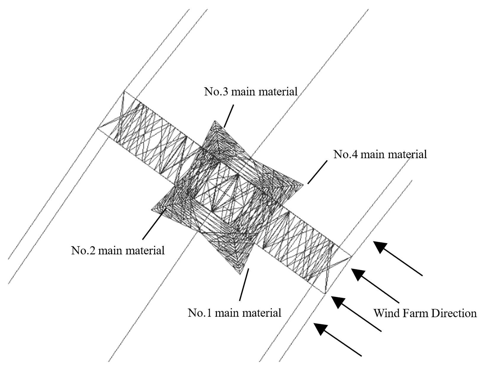
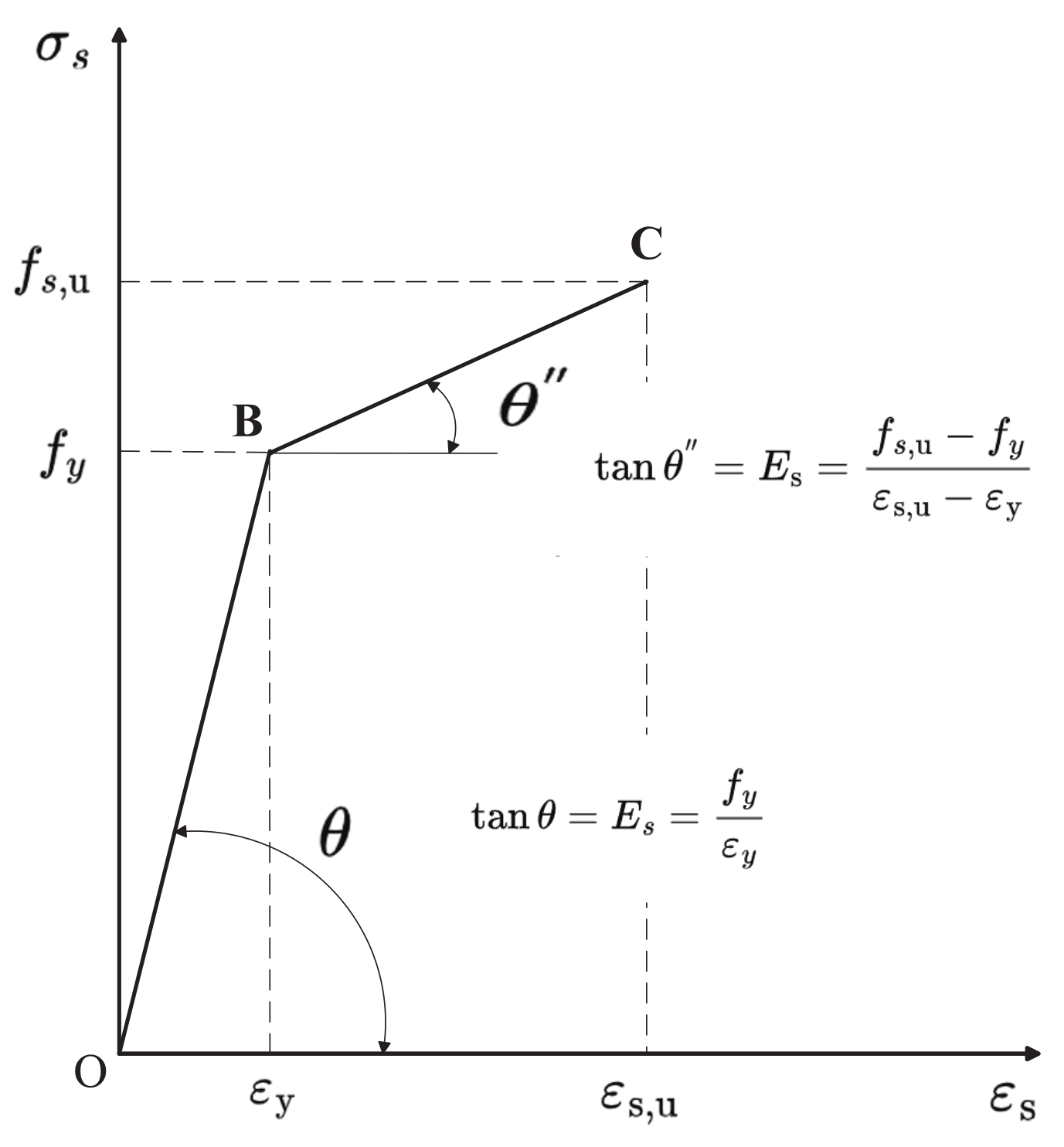
2.1. Transmission Tower Mechanics Simulation Model

This paper takes the data of a 220 kV mountain crossing line project in a certain place in Yunnan Province, China as the background. It carries out research according to the Chinese standard specifications, combined with the actual terrain conditions and parameters. The transmission towers on both sides of the transmission line are JBC1 cup-type tension towers, and the middle towers are ZBC1 tangent towers. The tangent tower has a total height of 40 m, and the tension-resistant transmission tower has a nominal height of 27 m and a total height of 32 m. According to the standard, the wind speed is 10 m above the ground as the design basis, the average maximum wind speed in 10 min is 27 m/s, the design maximum ice thickness of 30 cm.

Three towers and two lines of the actual operating line for the southwest-northeast direction, a typical over-the-hill type transmission line, are shown in Figure 1.

Tower 1# is the southwest transmission tower, and tower 2# is the transmission tower at the top of the hill. Tower 2# is 19.8 m higher in elevation than tower 1#. The distance between the two towers is 198.3 m. Tower 3# is lower in elevation, and its distance from tower 2# is 514.6 m. The difference in elevation of the hanging point is 48.6 m.

To facilitate the description of the later experimental results, the main materials of individual transmission towers are numbered separately, as shown in Figure 2. Each section of main material from the bottom of the tower to the top of the tower has a total of 30 beam units as axial force and wind direction observation points; the entire transmission line of 1, 4 main material for the windward side, and 2, 3 main material for the leeward side.The transmission tower single-line diagram is as shown in Figure 3.

Considering the force characteristics of the transmission tower and the bending moment of the angle steel, the B31 beam element and the T3D2 truss element are used to model the whole transmission tower, and the actual force of the transmission tower is simulated in detail. The experiment mainly uses Q345 and Q235 steel (

Table 1. Angle steel characteristics parameters.

Model	Density/(kg/m3)	Modulus of Elasticity/(MPa)	Poisson’s Ratio	Yield Strength/(MPa)	Tensile Strength/(MPa)
Q345	7750	206,000	0.3	345	551
Q235	7850	210,000	0.3	235	410

) to define different material properties to simulate the main material and diaphragm of the actual transmission tower.

Furthermore, in the construction of the simulation model, the steel is simplified as an ideal elastic–plastic material. It can be seen from the stress–strain curve of the steel during tension that the steel has a more obvious elastic and yield stage, but when the stress reaches the yield point, the steel strain can reach 2~3%. Although such a large deformation is not damaged, the structure or component is no longer suitable for continuing to bear the load, so the elastic–plastic stage is ignored, and the steel is simplified as an ideal elastic–plastic material.

As shown in the Figure 4. Take the slope of the BC line segment as 0.01E_s, and E_s is the modulus of elasticity of the steel. The yield strength of Q345B steel is 345 MPa, and the ultimate tensile strength can reach 510–600 MPa. The coordinates of point B are (345, 0), and the coordinates of point C are (551, 0.1). Make the slope between the two points 0.01E_s.

In the simulation, the spatial position of the beam element determines its stress state in the transmission tower system. By adjusting the normal direction of the beam element and the truss, the steel conforms to the real stress state of the transmission tower (

Table 2. Component size parameters.

Segment	Chord Member	Web Member	Segment	Chord Member	Web Member
1	L56 × 4	L40 × 4	6	L110 × 7	L65 × 5, L50 × 4
2	L70 × 5, L63 × 5	L45 × 4	7	L110 × 8	L63 × 5, L56 × 4
3	L75 × 5	L45 × 3	8	L110 × 10	L56 × 4, L50 × 4
4	L75 × 5, L70 × 6	L45 × 3	9	L110 × 10	L56 × 4
5	L75 × 5	L45 × 4	10	L125 × 20	L63 × 5, L56 × 4

).

In the experiment, the types of conductor and ground wire are steel-cored aluminum (strand JLG1A-400/35) and aluminum-clad steel (strand JLB20A-120), respectively. The specific physical parameters are shown in

Table 3. Physical parameters of conductors and ground wires.

Parameters	JLG1A-400/35	JLB20A-120
Cross-sectional area/(mm)	423.20	120.61
Outer diameter/(mm)	26.90	14.25
Mass per unit length/(kg·km−1)	1347.50	810.00
Modulus of elasticity/(MPa)	65,000.00	148,100.00
Rated breaking force/(kN)	274.3	217

.

The damping setting in the experiment is as follows. The damping of the transmission line adopts the Rayleigh damping assumption, and the use of Rayleigh damping is convenient. Compared with other forms of damping, the Rayleigh damping of each mode of the system can be accurately defined. The Rayleigh damping of each mode can be converted into direct modal damping, and the Rayleigh damping is converted into direct modal damping in Abaqus/Standard for dynamic calculation. The damping ratio of the two materials is different in much of the literature. In this paper, the damping of the conductor (ground) line is set in the simulation software. The corresponding parameter alpha value of the material damping is 0.229866, and the beta value is 0.00087. For a given mode i, the critical damping value is ${\xi }_i$, and the relationship between Rayleigh damping coefficient $\alpha$ and $\beta$ is

$${\xi }_i=\frac{{\alpha }_i}{2{\omega }_i}+2{\beta }_i{\omega }_i.$$

(1)

In Equation (1), ${\xi }_i$ is the critical damping, and ${\omega }_i$ is the natural frequency of the ith mode. It can be seen that the mass proportional damping part (${\alpha }_i$) of Rayleigh damping plays a dominant role in the low-frequency band of the system response, and the stiffness proportional damping part (${\beta }_i$) plays a dominant role in the high-frequency band.

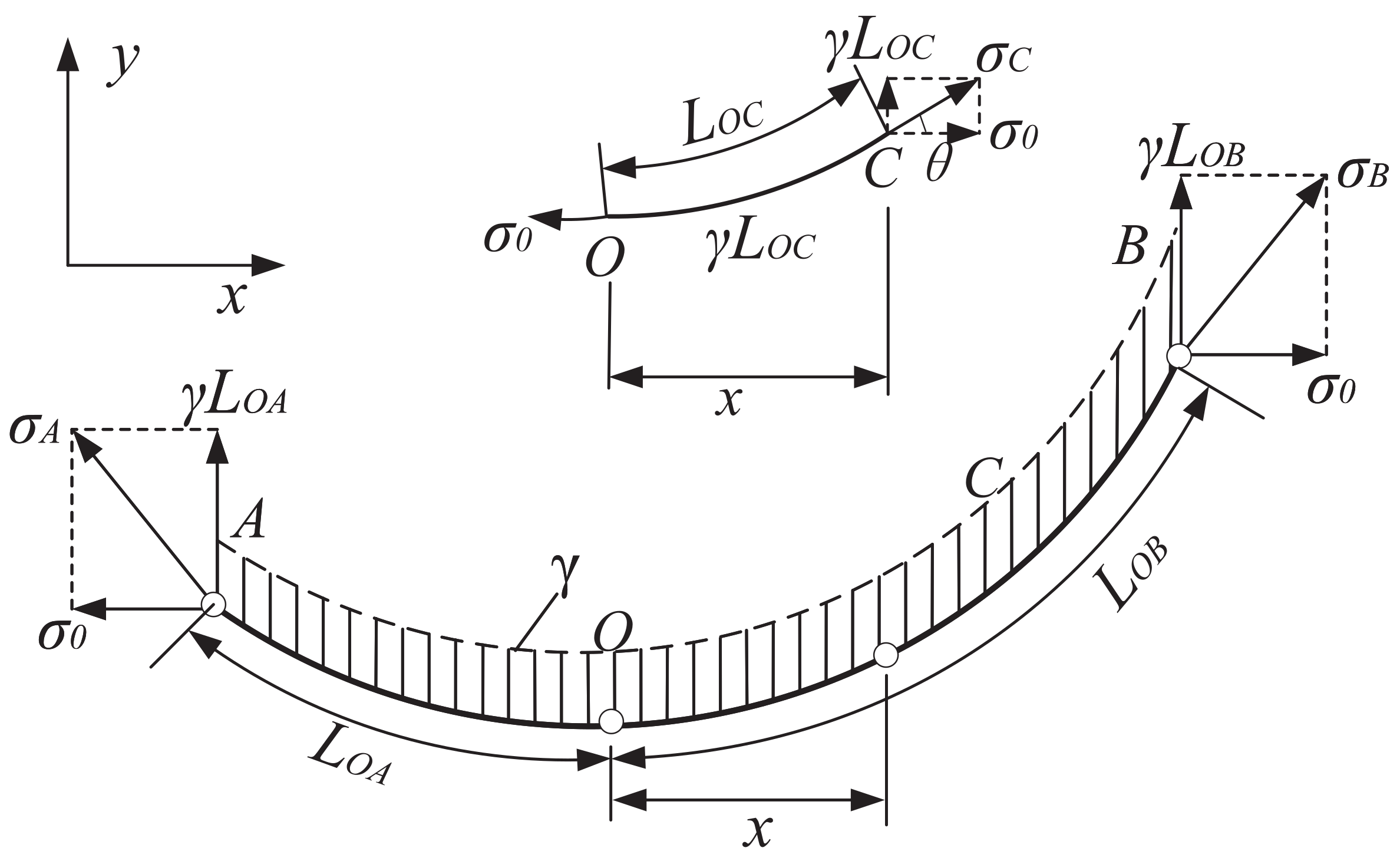
2.2. Conductor (Ground) Wire and Insulator String Modeling and Conductor (Ground) Wire Initial Form-Finding

After the finite element model of the transmission line is established, an essential prerequisite for analyzing the mechanical characteristics of the tower-line coupling system is the shape finding of the transmission line, and the nonlinear problem of the transmission line needs to be considered. Figure 5 shows the force analysis of the transmission line. Under the action of gravity and initial tension, the displacement and force of the transmission line will be redistributed so that the final force balance will be a suspended chain line.

Figure 5 shows the schematic diagram of the force analysis of the suspended messenger wire, where A and B points are the two suspension points of the transmission wire in the suspended state, and O point is the lowest point of the messenger wire. $\theta$ is the angle between the horizontal direction and the direction of the wire line, $\sigma$ is the unit stress value (MPa) of the transmission wire suspension line, and $\gamma$ is the load value (MPa) per unit area of the transmission wire cross section. For the analysis of the force situation of the whole section of the wire, the actual vertical load value of the suspension line is $\gamma$$\mathit{Loc}$, and the force analysis of the transmission wire can be obtained.

Figure 5A,B is the transmission conductor overhang state in the two ends of the suspension point, and the O point is the lowest point of the wire overhang chain. Among them, $\theta$ is the horizontal direction and the conductor along the direction of the angle, $\sigma$ is the transmission conductor overhanging chain-line unit stress value (MPa), and $\gamma$ is the transmission conductor cross-section unit area to bear the load value (MPa/m). The whole span of the wire to extract the cross-sectional unit stress analysis, the actual vertical load value of the suspension chain line $\gamma$$\mathit{Loc}$, and the transmission line stress analysis can be obtained. We have

$${\sigma }_{x}cos\theta ={\sigma }_0$$

(2)

$${\sigma }_{x}sin\theta =\gamma \mathit{Loc}$$

(3)

Equations (2) and (3) can be derived by dividing and simplifying. We have

$$tan\theta =\frac{\mathit{dy}}{\mathit{dx}}=\frac{\gamma }{{\sigma }_0}\mathit{Loc}$$

(4)

Differentiating and deforming the two ends of Equation (4), the general integral of the suspended chain line is obtained as follows,

$$y=\frac{{\sigma }_0}{\gamma }cosh\frac{\gamma }{{\sigma }_0}\left(x+C_1\right)+C_2$$

(5)

where cosh is the hyperbolic cosine function. The premise of the equation requires the left and right suspension points A and B. Consider the actual transmission line wire suspension points at both ends of the unequal height condition. The equation has certain application limitations. It is necessary to derive the line unequal height condition suspension chain-line equation. Set A, B as two suspension-point elevation differences for d through the coordinate offset, and they will be charged at the origin, and set the left suspension point A as the suspension chain wire OA horizontal distance to a. This will result in two points—coordinates (0,0), (a,0)—and in Equation (5) we will simplify the derivation of the transmission line by the suspension chain line basis of any two points A, B:

$$y=\frac{{\sigma }_0}{\gamma }\left[cosh\frac{\gamma (x-a)}{{\sigma }_0}-cosh\frac{\gamma a}{{\sigma }_0}\right]=\frac{2{\sigma }_0}{\gamma }sinh\frac{\gamma x}{2{\sigma }_0}sinh\frac{\gamma (x-2a)}{2{\sigma }_0}$$

(6)

The sinh in the equation is the hyperbolic cosine function.

From the above analysis of any two points of the suspension chain-line base equation, in the process of overhead transmission line modeling, it is necessary to first determine the coordinate position of the transmission line suspension point. To bring the coordinates at each end of the suspended chain line obtained above into accord with three-dimensional spatial coordinates, determine the spacing between the wires and ground spacing, and select the suspension state of the broken chain-line equation according to the operating parameters of the line.

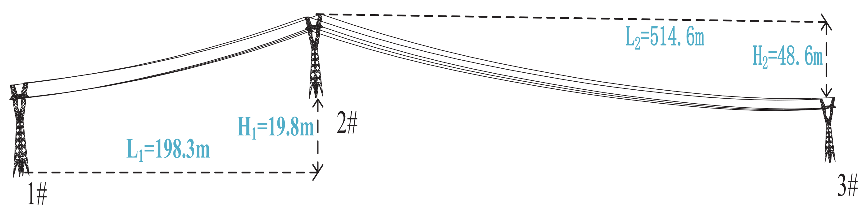
2.3. Large Stall Distance and Large Height Difference Defined

Transmission lines of large height difference and large span difference still need to be clearly defined. The actual use of the tower height difference coefficient is used to determine whether the transmission line has a large height difference or a large span distance difference that is more in line with the definition of the tower height difference coefficient. We have

$$\alpha =\frac{H_1}{L_1}+\frac{H_2}{L_2},$$

(7)

where the $\alpha$ value is greater than 0.2—that is, the transmission line belongs to the case of large height difference. Think of the ratio of both sides of the straight span distance $L_2$:$L_1$ as being greater than 2 for the case of large span distance differences. Furthermore, an $\alpha$ value greater than 0.2 and an $L_2$:$L_1$ ratio greater than 2 is regarded as a large difference in height with large span difference conditions that are not satisfied. The above situation is not a large difference in height with nonlarge span difference conditions.

2.4. Nonlinear Equations for Tower-Line Coupled Systems

The whole system of transmission tower lines has the characteristics of strong nonlinearity, rigid–flexible coupling, large span, and a large elevation difference. When wind and ice loads are applied to the coupling system, the overall structural condition of the transmission tower will change more significantly, which in turn causes changes in the axial force and tension of the transmission tower-line system, so it is necessary to consider the complete tower-line coupling system in the analysis process. In the simulation system analysis, the stiffness matrix of the unit is assembled into the total stiffness matrix of the transmission line, and the overall displacement of the transmission line node is the unknown solution to establish the general equilibrium equation set of the transmission tower-line system. We have

$$\left(\left[K_{\mathrm{E}}\right]+\left[K_{\mathrm{G}}\right]+\left[K_{\mathrm{NL}}\right]\right)\left\{U\right\}=\left\{F^0\right\}+\left\{F\right\}+\left\{R\right\},$$

(8)

where $K_E$ is the overall elastic stiffness matrix of the transmission line system, $K_G$ is the total stiffness matrix of the coupling system, $K_{NL}$ is the initial displacement matrix of the transmission line, U is the displacement vector of the node to be solved for the coupling model, $F^0$ is the initial force vector of the nodes of the coupling system, F is the unbalanced force vector of the nodes of the coupling system, and R is the load vector of the nodes of the coupling model.

This nonlinear dynamic equilibrium equation can be calculated by using the simulation system calculation program and the equilibrium iteration method to achieve a strong equilibrium convergence of the load end solution. At the same time, the system completes the iteration and activates the large deformation effect of the transmission line tower-line coupling system model through the node and unit force analysis and displacement change, while the values of axial force and stiffening effect can completely guarantee the reliability and accuracy of the simulation model.

2.5. The Main Analysis Steps of the Experiment

The main analysis steps of simulation are as follows.

Step 1: Form-finding under static force. The four legs of the three transmission towers are completely fixed, and then the gravity is applied to the transmission tower line as a whole, and the axial force of the main material and the initial tension of the transmission line under gravity are analyzed (static, general).

Step 2: Apply the corresponding wind–ice load to the conductor to explore the steady-state characteristics of the transmission tower line (static, general).

Step 3: Remove the iced truss element to simulate the whole process of conductor ice shedding. The analysis is performed to open the large deformation switch (dynamic, implicit).

Step 4: Analyze the dynamic response of the transmission tower-line coupling system to ice shedding (dynamic, implicit).

In order to facilitate the subsequent researchers to reproduce the experiment, the INP file of the main process of the simulation experiment is shown in Appendix A.

3. Wind–Ice Load Loading Method in the Experiment

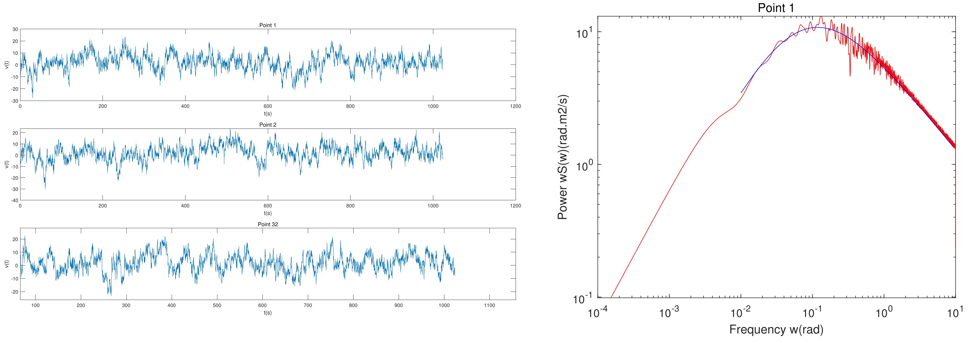
3.1. Wind Load Characteristics Analysis

In the simulated wind speed time history sample, this paper uses the harmonic superposition method to simulate the fluctuating wind, and uses matlab to convert the wind-speed time history sample established by fluctuating wind and average wind fitting into wind load.

The traditional values of horizontal wind loads on conductors and ground lines are calculated according to GB50545-2010 Technical Specification for the Design of 110 KV–750 KV Overhead Transmission Lines. We have

$$W_x=\alpha ·W_0·{\mu }_z·{\mu }_{sc}·{\beta }_c·d·L_p·B·{sin}^2\theta$$

(9)

$$W_0=v^2/1600$$

(10)

where $W_x$ is the standard value of the guided ground load (kN), $\alpha$ is the wind pressure unevenness coefficient, ${\mu }_{sc}$ is the conductor body type coefficient, ${\beta }_c$ is the wind load adjustment coefficient of the conductor, d is the outer diameter of the conductor or the calculated outer diameter when icing (m), a split conductor is the sum of the outer diameter of all subconductors, ${\mu }_z$ is the wind pressure height coefficient, v is the essential design wind speed (m/s), and $\theta$ is the angle between the wind direction and the direction of the conductor.

The wind load model of transmission pylons is calculated as follows,

$$W_i={\mu }_{si}·A_{si}·v_i^2/1.6,$$

(11)

where $W_i$ is the wind load (kN) obtained for each tower section, ${\mu }_{si}$ is the body coefficient of the transmission tower, $A_{si}$ is the projected area of the tower body in the wind load calculation, and $v_i$ is the wind speed at the location of each tower section.

The transmission tower-line structure model is complex, and the single transmission tower nodes reach 2842. According to the area attached to the tower-line system, the wind is applied to the critical nodes. The selection of the key nodes in the transmission tower along the line direction key nodes 56 and 27 are perpendicular to the conductor direction in Figure 6. Figure 6 shows the wind spectrum course of imposing some key nodes. We verify the validity and reliability of the simulation pulsating wind method as shown in Figure 6.

The wind load is applied to the transmission line at its median height. This is the “median height” calculation method in which the span of suspension points at both ends of the transmission line divided by the integral of the height difference between each point and the lowest point of the wire along the wire When the wireline is a suspended chain line, in engineering applications, the median height of the transmission line is generally available in the following formula,

$$h_{av}\approx \frac{1}{3}{f}_m+\frac{{\sigma }_0}{2\gamma }{\left(\frac{h}{l}\right)}^2,$$

(12)

where $f_m$ is the maximum arc sag of the wire, and $h_{av}$ is the median height of the wire. From Equation(5), the suspension chain-line base equation can be derived from the wire arc sag:

$$f\left(x\right)=\frac{H}{L}x-\frac{2{\sigma }_0}{\gamma }sinh\frac{\gamma x}{2{\sigma }_0}sinh\frac{\gamma (x-2a)}{2{\sigma }_0}.$$

(13)

3.2. Simulation Method for Dynamic Response of Conductor Overlay (De)ice

The actual ice-covered cross-section of the power transmission line is an irregular “new moon” shape. The traditional method employed for calculating the weight of water on an ice-covered line was to use the water level method. However, in this experiment, research revealed that in the calculation of ice cover and in finite element simulation, the difference between the irregular and regular ice-covered surfaces is about 5%. It can be assumed that the ice is uniformly distributed over the surface of the overhead line. In order to more realistically take into account the inertia effects of the ice, Abaqus was used to simulate the ice cover on a power transmission line by using a pipe section. In order to realistically simulate the mechanical interaction between the ice and the conductor, Abaqus was also used to set up beam elements with junctions between the conductor, ground wire, and bridge elements. The physical parameters of the ice were taken to be the elastic modulus of 100 MPa with a density of 0.9 kg/m³. The process of ice shedding from the conductor was simulated by using the program in Abaqus. The activation or deactivation of elements at different steps was used to simulate the process of ice cover and ice shedding through the analysis step in the activation or closure. The transmission lines’ ice-shedding load curve is shown in Figure 7, where $F_{load}$ is the total gravity load of the wire and overlying ice before ice shedding; killing the overlying ice beam unit process at the moment of $t_0$ is the moment of wire ice shedding; $\alpha$ is the ice-shedding rate and ($1-\alpha$) $F_{load}$ is the load applied to the wire after ice shedding.

4. Experiment Design and Analysis

The transmission line experiment is a simulation of the actual transmission line, mainly for the large height difference, large stall distance difference, wind and ice load stability, and transient conditions for analysis. The object of study is a typical mountainous overhill-type transmission tower-line coupling model of three towers and two lines. According to the actual terrain conditions combined with the above definition of large height difference and large stall distance difference, different wind and ice load levels, elevation difference, and large stall distance differences are set in the simulation model, and comparative experiments are established.

4.1. Analysis of Steady-State Calculation Results

From the previous mountain transmission line accident analysis, it is known that the main reason for the accident is the transmission tower in the wind and ice load superposition factor condition, coupled with the existence of the difference between the transmission line’s large span distance and large stall distance, which results in the transmission tower’s force steady-state imbalance, broken lines, a fallen tower, or other accidents. First, apply a gravity load to the tower and line coupling system, analyze the force state of the tower under the overall stability, and extract the main shaft force of each tower, respectively, as shown in Figure 8 (left). The unit number of the main material group of a single tower is marked in Figure 8.

The monopole tower is only symmetrical under gravity, so only the main material of tower 1# is considered in the calculation. The transmission tower is analyzed by comparing the tower–wire coupling system with no wires through the analysis of Figure 8. The analysis of Figure 8 can be obtained with regard to the transmission tower’s conductor state to consider the tower-line coupling system compared to a no-conductor state. Axial force changes significantly. The maximum axial force in the 3# tower height is 4.2 m with regard to main material a, with the conductor contribution axial force accounted for being 78.4%. Further analysis found that the same transmission tower under the action of gravity changes on both sides of the conductor axial force due to the influence of the wire factors, leading to the existence of the transmission line direction of the moment. Specifically, the 1# transmission tower (1, 2) has a main material positive value for tension, and (3, 4) has a main material negative value for pressure. In addition, the 2# transmission tower, due to the left side of the 198.3 m span distance and the right side of the 514.6 m large span distance gap, has axial force characteristics and is similar to 1# transmission tower. In addition, we have the 3# transmission tower (1, 2) main material’s left side of the large span distance. Of the (2) main materials on the left side, there is a large span distance difference, resulting in the maximum opposing axial force of the transmission line, and (3, 4) main materials produce the maximum positive tension. The experiment further analyzes the wind–ice load on the transmission tower single tower and tower-line coupling steady-state impact. Set the ice thickness at 15 cm, and the ice thickness values refer to “heavy ice overhead transmission line design technical regulations”, with a wind load of 15 m/s. Then, extract the wind–ice load transmission tower’s line of axial force distribution as in Figure 9.

In Figure 9, the wind–ice load model calculation results can be seen. Due to the wind–ice load under the action of the overall moment’s decision, the transmission tower’s windward side has an axial force that has positive tension, and the leeward side of the tower axial force has negative pressure. The windward side (1, 4) of the tower around the total value of the tensile force is less than the same tower’s leeward side (2, 3) with regard to the main material’s ability to bear pressure. Further analysis shows that in the same transmission of the same side of the tower’s main material axial force, there are also differences. The most significant difference for the 3# tower, and the comprehensive comparison of wind load without a wire model can be seen in Figure 9’s calculation results, which are the result of wind and ice load and common wire action.

Due to the local acceleration effect of the mountain uphill, the hilltop 2# transmission tower’s location is at a relatively higher elevation with higher wind speed. The tower’s wire suspension point is small around the two sides of the axial force difference. The wind–ice load and large span difference between the large elevation difference is caused by the joint action of this hilltop transmission tower. Furthermore, the main material maximum axial force exists in transmission tower 3#, where the transmission line and large span difference between the large elevation difference impact are more significant than the wind–ice load. A comparison of the above, with and without wind–ice load and single tower transmission tower at the axial force, is shown in

Table 4. The effect of conductor and wind–ice load on the main material axial force of transmission tower.

3# Tower Main Material Number	Self-Weighting without Wires/(N)	Wind Load without Conductor/(N)	Wind Load Axial Force Contribution	Self-Weighting with Wire/(N)	Wind and Ice Loads with Conductors/(N)	Axial Force Contribution of Wind and Ice Loads
1	−15,601.2	26531	62.97%	−298,136	−278,609	7.01%
2	−15,757.9	−58,197.5	72.92%	−293,839	−392,093	25.06%
3	−15,679.4	−57,466.3	72.72%	267,660	247,628	8.09%
4	−15,657.5	27,192.6	63.46%	264,024	364,672	27.60%

.

Through Table 4, it is obvious to see that the wire for the main material axial force contribution is the largest. Wind load on the transmission tower axial force contribution rate can also all reach greater than 62%, where the main material 2 and 3 wind load on the transmission tower axial force contribution are greater than 72%, wind load under the action of the leeward side of the axial force has the most significant impact. The contribution of wind and ice loads together on the axis force of main material 4 is 27.60%.

Therefore, in the actual mountain transmission line construction, the transmission tower should be fully considered with regard to both sides of the stall distance difference and the impact of wind–ice load. We try to avoid setting a large span distance in mountainous areas with high wind speed, which is conducive to reducing the transmission tower axial force and guiding the wind-generated parallelepiped tension difference on both sides to ensure the safe operation of transmission lines.

4.2. Analysis of Ultimate Bearing Capacity of Tension Tower

In general, the triggering factor of the transmission tower collapse caused by wind–ice load is the buckling of compression members. In the model, the influence of the buckling effect in nonlinear static analysis is considered. On the other hand, the critical initial imperfection is also concerned—that is, the initial bending shape is set to the first-order modal shape of its characteristic buckling, and the corresponding amplitude is set to $L/1000$.

Considering the effect of installation errors and other random factors, the initial geometric shape of the tower is corrected by a first-order bending mode shape, with the corresponding amplitude set to H/1000. Additionally, in order to account for the nonlinear effects of the material, the limit loads for the tower frame under different distributions of wind and ice loads are analyzed. The limit loads for a displacement-type transmission tower under different distributions of wind and ice loads are shown in Figure 10.

As shown in Figure 10, the damage to the top of the tower in both cases is triggered by member buckling at a height of about H/3 above the ground. The maximum wind speed in the final state is 29.6 m/s, which is close to the maximum wind rating of 27 m/s for the actual transmission tower design, The ultimate bearing capacity of the transmission tower is 545.5 kN.

The tower foot upper member in the figure from 1.15 s onward can be seen to lose its carrying capacity, after which the pressure transmission path is cut, and the tension member is bent directly. On the other hand, since the load cannot be transferred to the path that has been cut, the tower leg undergoes slight deformation. Consequently, this tower has almost no resistance to progressive collapse. In 2019, a tower in Yunnan province collapsed in an ice- and wind-prone area. The strain section of an electric transmission line project in the area collapsed, and the tower frame and the main stringing conductor of the collapsed tower were similar to the tower in the present experiment. The collapsed tower’s arms with the guide wires were inserted perpendicularly into the ground in the direction of the collapse, the main chord members and the web members were bent, and the tower foot and the foundation did not show significant damage, similar to the results of the present analysis.

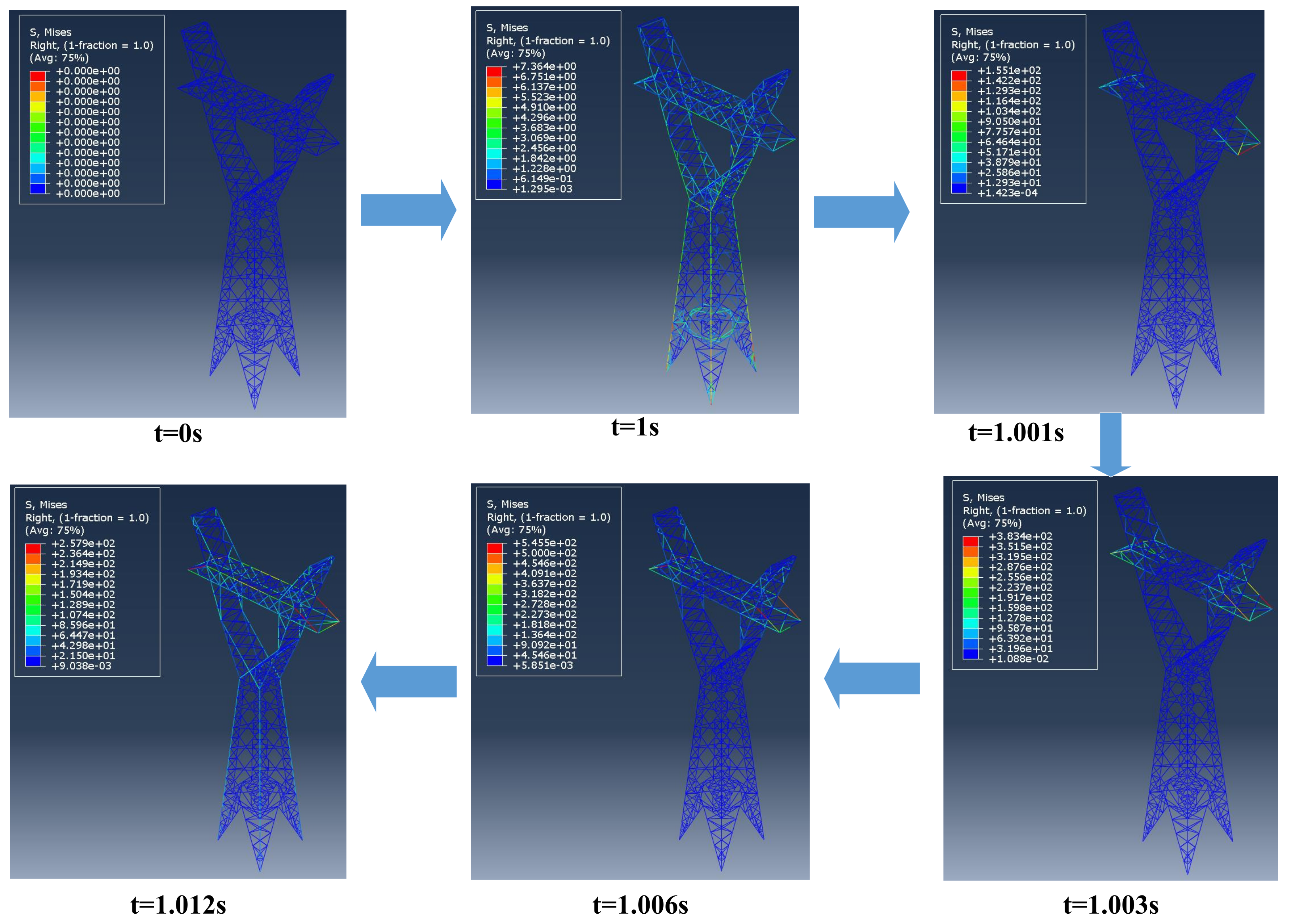
4.3. Analysis of Transient Calculation Results

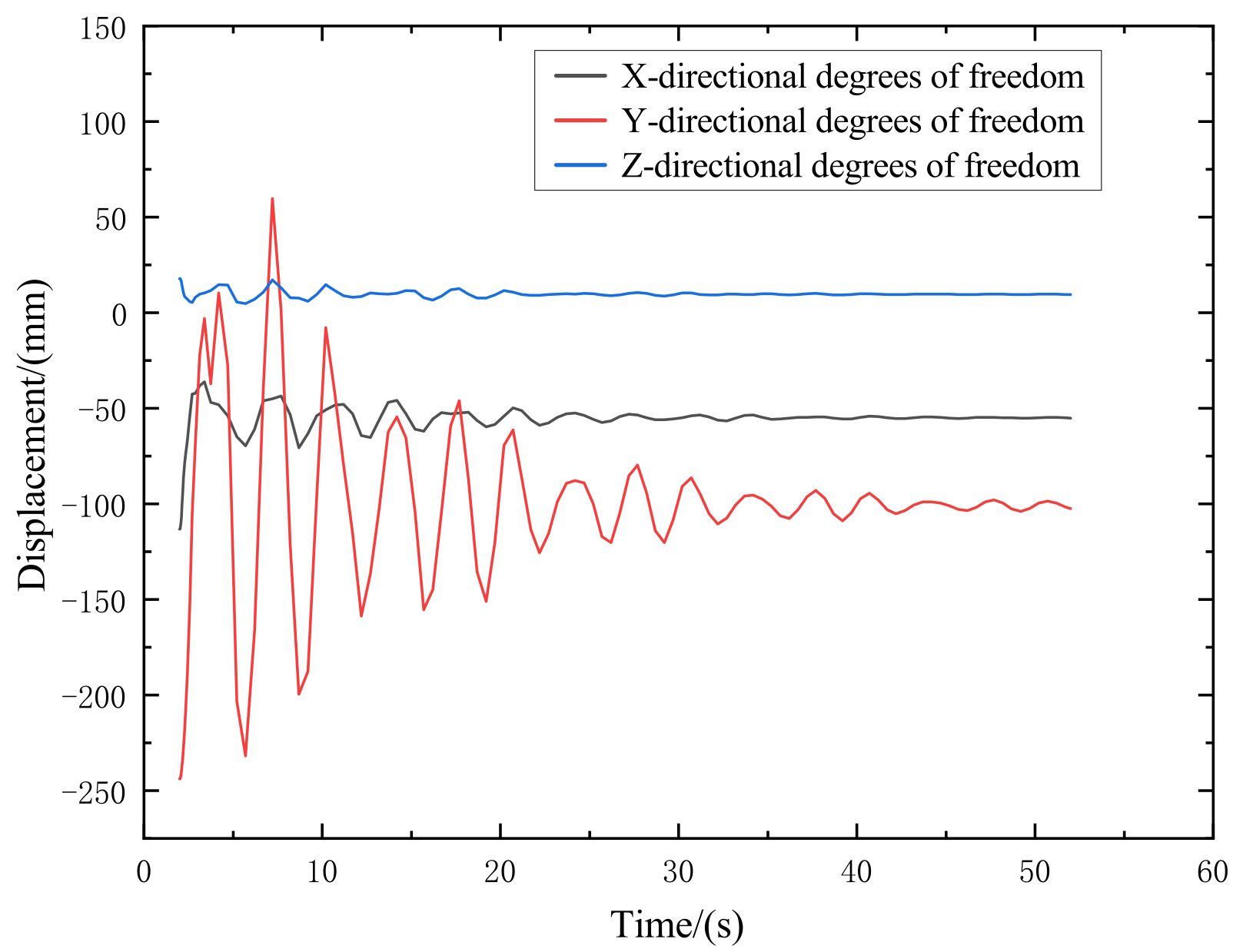
4.3.1. Characterization of Wind-Ice Load Dynamic Response

Transmission towers with a wind-ice load, and a conductor undergoing ice shedding, will not only experience lateral oscillation but also produce a free oscillation effect. Consequently, there is a need for the wind-ice load in the conductor ice-shedding dynamic response model for computational analysis. The actual transmission line data for three towers and two lines was a 198.3 m span distance, a 514.6 m continuous span distance, a transmission guide, and a ground line ice thickness of 20 cm. The conductor for the whole-span, ice-shedding numerical simulation of wind-speed levels were 5 m/s, 10 m/s, 15 m/s, 20 m/s, and 25 m/s. The large span distance side of the transmission line in the time course of the vertical direction of ice-shedding displacement, is shown in Figure 11.

In Figure 11, it can be seen that the wind speed on the transmission line ice-shedding vibration is not apparent and mainly affects the final swing position of the transmission line. A wind speed greater than 10 m/s after the final swing position increased significantly, with the maximum increase being of 39.7%, and 20 m/s after the increase decreases, the wire is over the ice, and the ice shedding the maximum jump height is of 11.13 m.

The highest point of the second tower’s no. 1 node is further extracted over the top of the mountain, and the wind load and ice-shedding state of its three degrees of freedom displacement analysis (Figure 12) can be seen in the lateral swing of X degrees of freedom displacement. Along the wire direction of Y degrees of freedom, displacement by the wind speed is evident. The increase in wind speed and increase in the maximum lateral swing is 4.2 times along the wire direction.

The wind-ice load input and ice-shedding experiment were further analyzed to investigate the force characteristics and force transmission of the transmission tower under wind-ice load. The time-varying stress cloud diagram of the transmission tower was plotted when it was under the wind-ice load, as shown in Figure 13.

Figure 13 shows that in 1 s, the transmission tower line is subjected to a more uniform force under gravity, and the maximum force is concentrated at the tower foot. After 1s, the transmission line is subjected to the wind-ice load simultaneously, and the stress at the position of the cross-beam begins to increase gradually. The stress then propagates to the main body of the transmission tower through the cross-beam in a very short time. The stress cloud diagram at 1.012 s shows the stress distribution after the propagation. However, the stress is still the maximum at the cross-beam. Therefore, for the transmission tower with a linear shape, the key part for the stress distribution needs to be reinforced, and the transmission tower in the area with a high wind speed needs to be monitored closely. Ice should be melted promptly, but also in such a way as to avoid the short-term strong ice removal that may cause the stress of the transmission tower components to be too large and lead to failure.

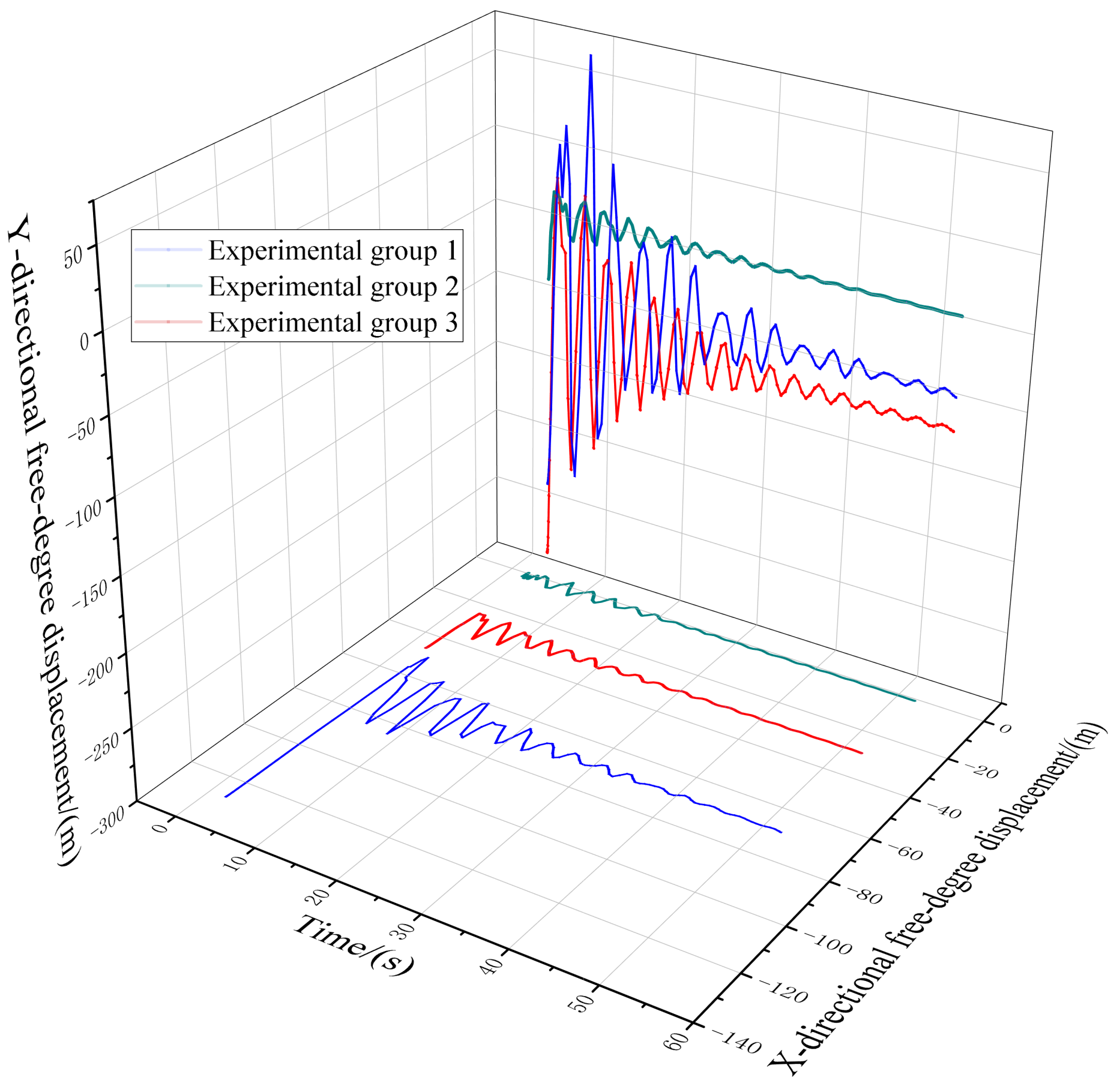
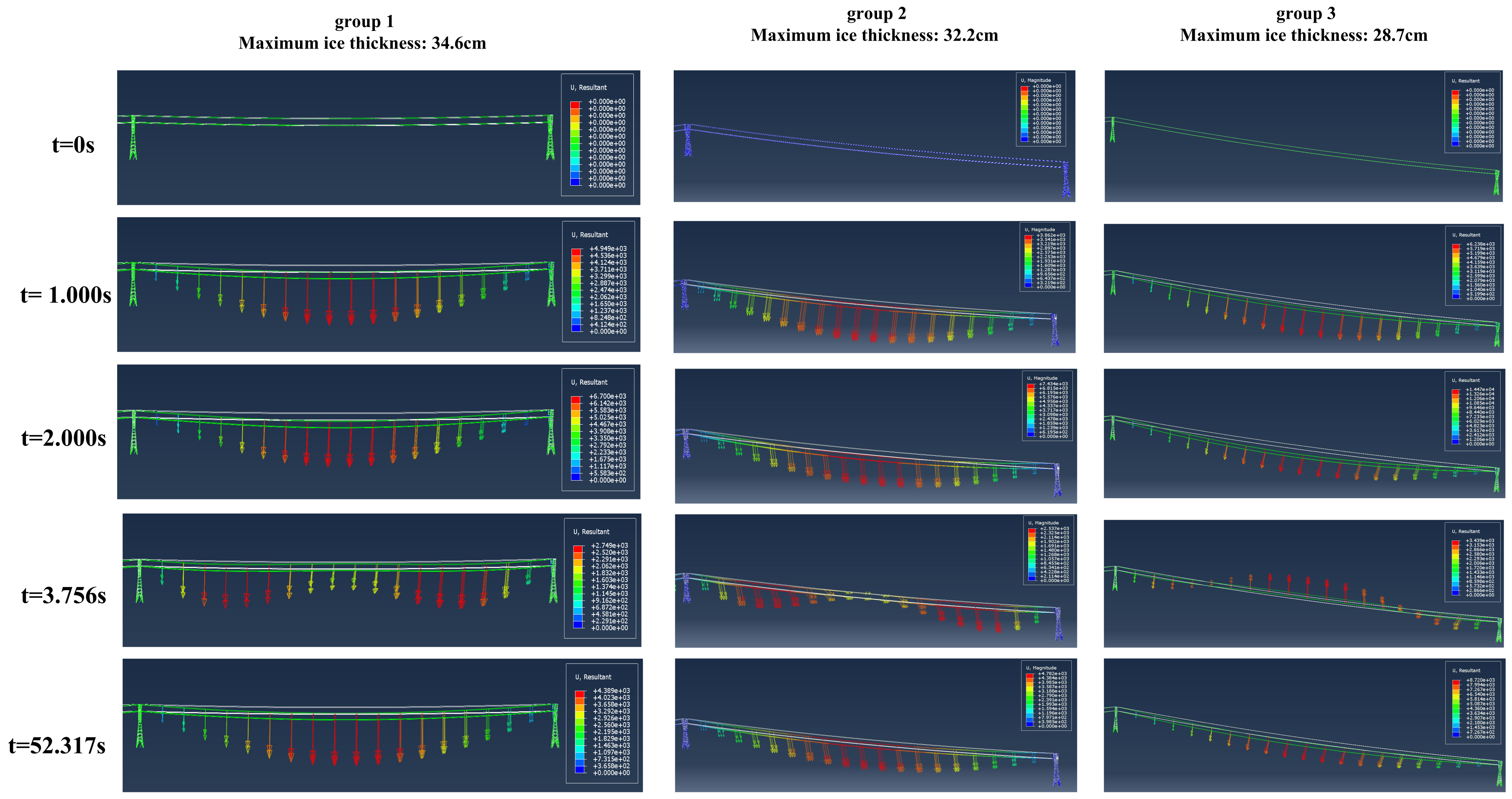
4.3.2. The Effect of Large Height Difference and Large Stall Distance Difference

Given the environmental factors of large span differences and large height differences in mountainous areas, the relevant comparison experiments are selected for tower-line coupling model analysis to study the state of force and influence law of transmission line ice-shedding jump under different span distances and height differences. In the experiment, the ice-shedding rate is 100%, the thickness of the transmission line ice is 20 cm, and the wind speed is 15 m/s. The parameters of the simulation model are shown in

Table 5. Comparison model parameters.

Group Name	Stall Spacing ${\mathit{H}}_1$	Stall Spacing ${\mathit{H}}_2$	Elevation Difference ${\mathit{L}}_1$	Elevation Difference ${\mathit{L}}_2$
Group 1	350 m	350 m	0 m	0 m
Group 2	350 m	350 m	19.8 m	48.6 m
Group 3	198.3 m	514.6 m	19.8 m	48.6 m

.

$L_1$, $L_2$, $H_1$, $H_2$ in the Table 5, refer to Figure 1,Calculated in the case of the above three groups of parameter models are the different line stall distances under the conductor shedding ice at the transmission tower’s highest point lateral to and alongside the line swing displacement. The initial tension of the conductor corresponding to the three groups of models is 46.54588 MPa, 48.33 MPa, and 67.23 MPa, respectively.

After the above analysis, in the wind-ice load, ice shedding occurs mainly on the transmission tower’s transverse swing and along the wire direction’s swing amplitude with regard to the most significant impact on the vertical direction of the tower body axis force. Here, the focus of the analysis is on the large span distance difference between the large height difference on the transmission tower transverse and along the line direction swing. As shown in Figure 14, three groups of tower-line coupling models (in the case of different line spacings of the transmission tower’s highest point-transverse and along the line swing displacement time range calculation curve) can be obtained. Here, X degrees of freedom (transverse swing) and Y degrees of freedom (along the transmission line direction) can be seen in the span spacing; the greater the elevation difference, the greater the swing of the wire in the process of ice shedding. However, in Figure 11, it can be seen that the influence factor of the lateral swing is the largest in the elevation difference; in the direction of the transmission line, the swing along the large stall distance difference influence factor is the largest.

Figure 15 shows the complete stall distance ice-shedding process and the transmission line ice-shedding maximum tension time range change curve. Through the analysis, we can see that the transmission line produces the maximum tension point for the insulator at both ends of the transmission line connected to the tower. Wind-ice load, with regard to the tower-line coupling system, dictates that the more incredible the span distance, the greater the amplitude of the transmission line off the ice. In addition, the greater the amplitude of tension change, the maximum tension growth value will be of 59.58%. Consequently, the design of the transmission tower process should be based on the actual mountain and climate environmental factors so that the transmission line can ensure line safety.

The analysis of the power transmission line in the large span difference and high-altitude difference shows that the maximum ice thickness of the conductor changes with the change of the large span difference and high-altitude difference. In the finite-element model, the stress distribution under the wind–ice load is satisfied with the design stress limit as the criterion, and the limit ice thickness of the conductor can be calculated. The time-arc-cloud diagram of the power transmission line under the limit of ice thickness is shown in Figure 16.

The analysis of the maximum time history-conductor sag under the load of gravity for the three groups of experiments in Figure 16 is as follows. The maximum time history-conductor sag under the load of gravity for the third group of experiments is 6.238 m within the first second, followed by the second group of experiments with only the height difference, with a conductor sag of 3.541 m. The difference between the two groups is significant when only the difference in the large interval is considered. When the ice load is removed at the second second, it can be seen that the frequency of oscillation of the transmission line for the third group of experiments is lower than that of the other two groups. The conductor sag of the third group of experiments stabilized at 8.72 m in the end, which is the result of the combined action of the large interval difference and the wind load. Additionally, from the simulation results, it can be seen that the interval difference directly affects the maximum ice thickness on the transmission line. The transmission line with a large interval difference and a large height difference will have a maximum ice thickness that is lower than the design maximum ice thickness.

4.3.3. Analysis of Transmission Tower-Line Safety under Wind-Ice Coupling

In mountain transmission lines, the design stiffness of the transmission tower is much greater than the maximum tension value of the guide and ground wire-the wire under a single external load on the transmission line caused by a controlled impact–esulting in the study of transmission tower line safety issues. This often ignores the coupling effect of multiple external loads. In particular, the mountain transmission tower line easily produces a large external transient load, resulting in the conductor ice-shedding process due to changes in tension, which will produce substantial impact damage to the transmission tower and result in major accidents, such as broken lines and inverted towers.

The above has established the transmission tower-line coupling system simulation model to ensure the safety of the transmission line design, based on simulation analysis to calculate the transmission lines under wind–ice loads, their own gravity under the maximum tension, and tower axial force, combined with transmission tower-line safety standards. The established transmission tower security posture warning chart is seen in Figure 17.

In transmission towers, whether of large or small stall distance, if only a single side of the external load is applied, the transmission line will collapse when the transmission conductor reaches the pull-off force. When both sides of the transmission tower apply the load at the same time, the final large span distance side of the pulling force will play a decisive role in the transmission tower safety posture. Continued application of force will result in an inverted tower accident because the left and right sides of the load neutralization will be maintained in the safety threshold, as the large stall distance side of the pulling force will continue to increase.

5. Conclusions

This paper takes a mountainous transmission line in Yunnan as the background and establishes the actual working conditions of the three towers and two wires of a tower-line coupling system finite-element calculation model, fully considering the operation of mountainous transmission lines under wind and ice loads. The conclusions are as follows.

(1)

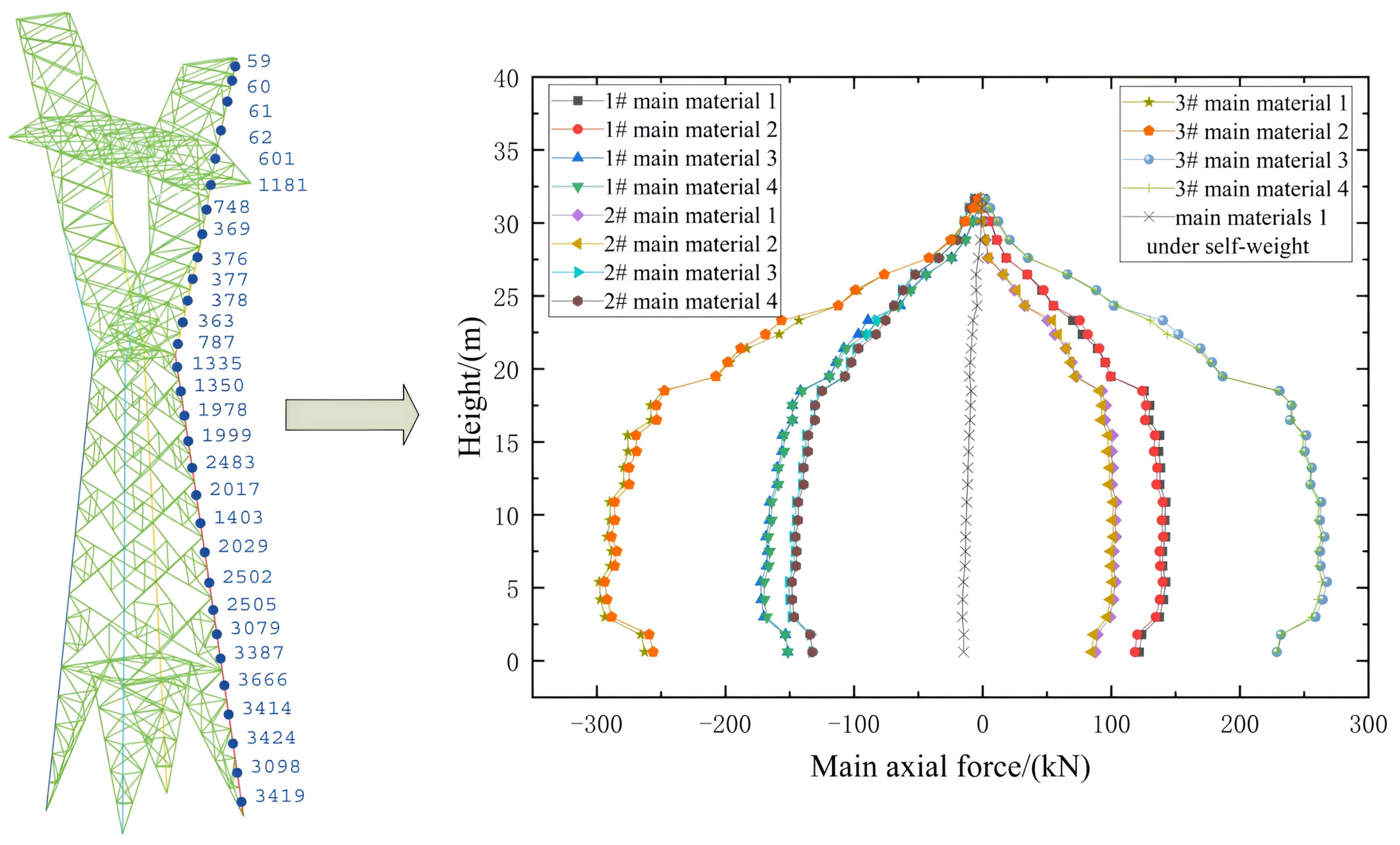
For transmission lines in mountainous terrain, under the static conditions of self-weight and wind-ice load, compared with no conductor, the axial force changes significantly, and the highest contribution rate of conductor axial force is 78.4%. The maximum value-added of wind-ice load on the basis of the contribution rate of the conductor is 27.6%, and the wind-ice load has a significant impact. The axial force of the tower main material mainly changes on the leeward side.

(2)

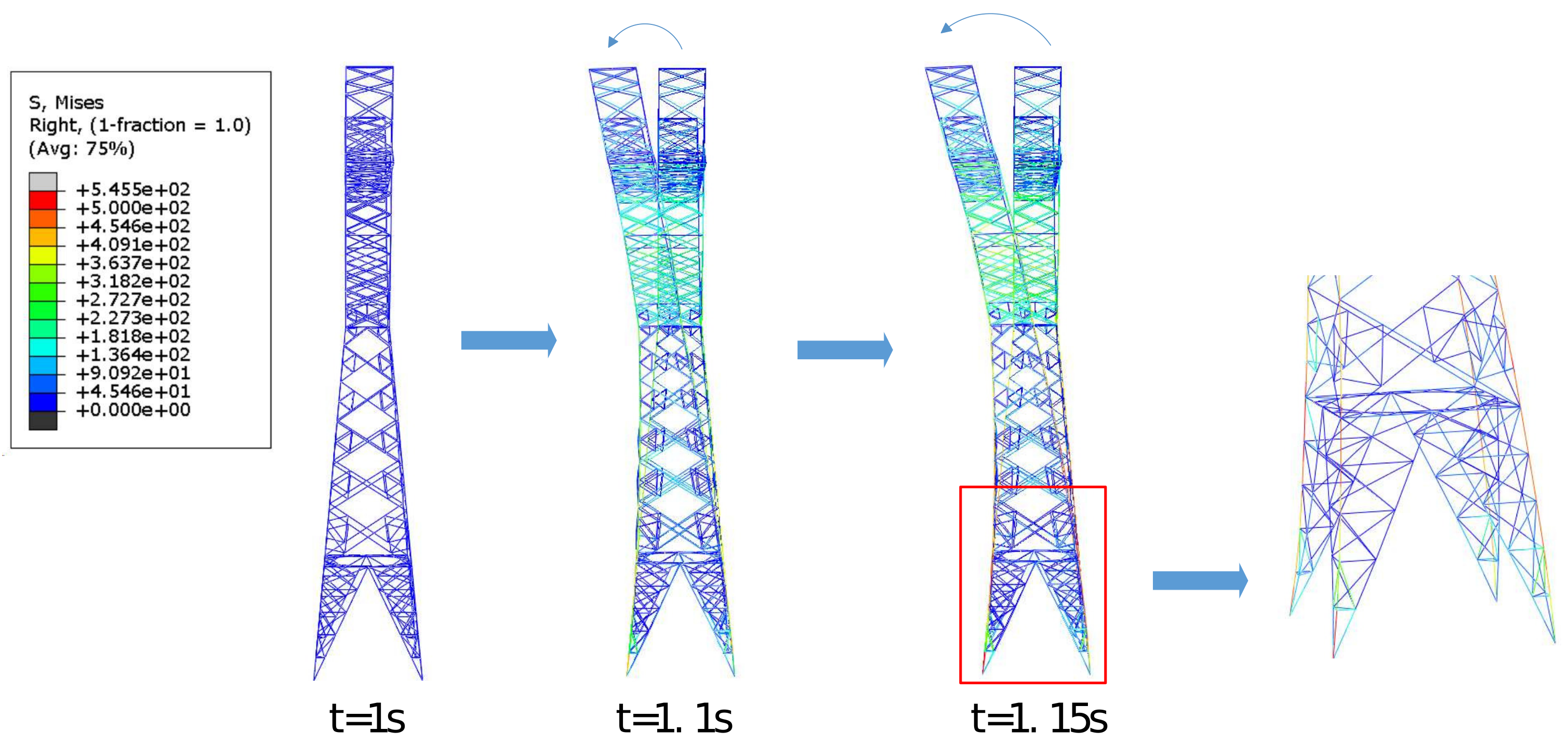
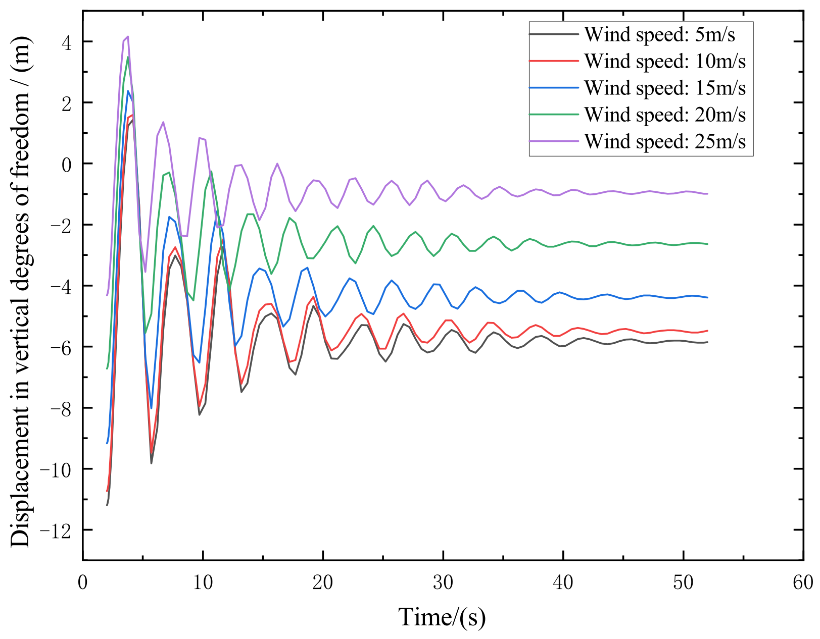
Considering the transmission tower-line coupling system model under the transient ice-shedding load of wind and ice, the dynamic response load of the axial force is significantly larger than the calculation result under the steady-state condition. In the experiment, under the large span difference and large elevation difference, the ice-shedding jump height of the conductor is the maximum of 11.13 m. The wind load has little effect on the vibration frequency of the conductor and has a greater effect on the stress vibration in the axial direction and the vertical line direction.

(3)

The maximum tensile strength of the tension tower is 545.5 kN, and the amplification effect of pulsating wind and conductor ice-shedding on the dynamic response of the line should be fully considered in the actual working condition. The large elevation difference mainly affects the tension in the X and Y degrees of freedom, and the maximum tension increase is up to 59.58%. Through the force transmission analysis of the straight tower, the position with the maximum bearing capacity is determined, and the main material should be reinforced at the cross-beam. Further analysis of the maximum ice thickness of the transmission line under the mountainous environment with large elevation difference and large span difference shows that it is smaller than the design value. The transmission line should pay attention to the influence of the mountainous terrain on the wind and ice load of the line, and reserve enough threshold space.

(4)

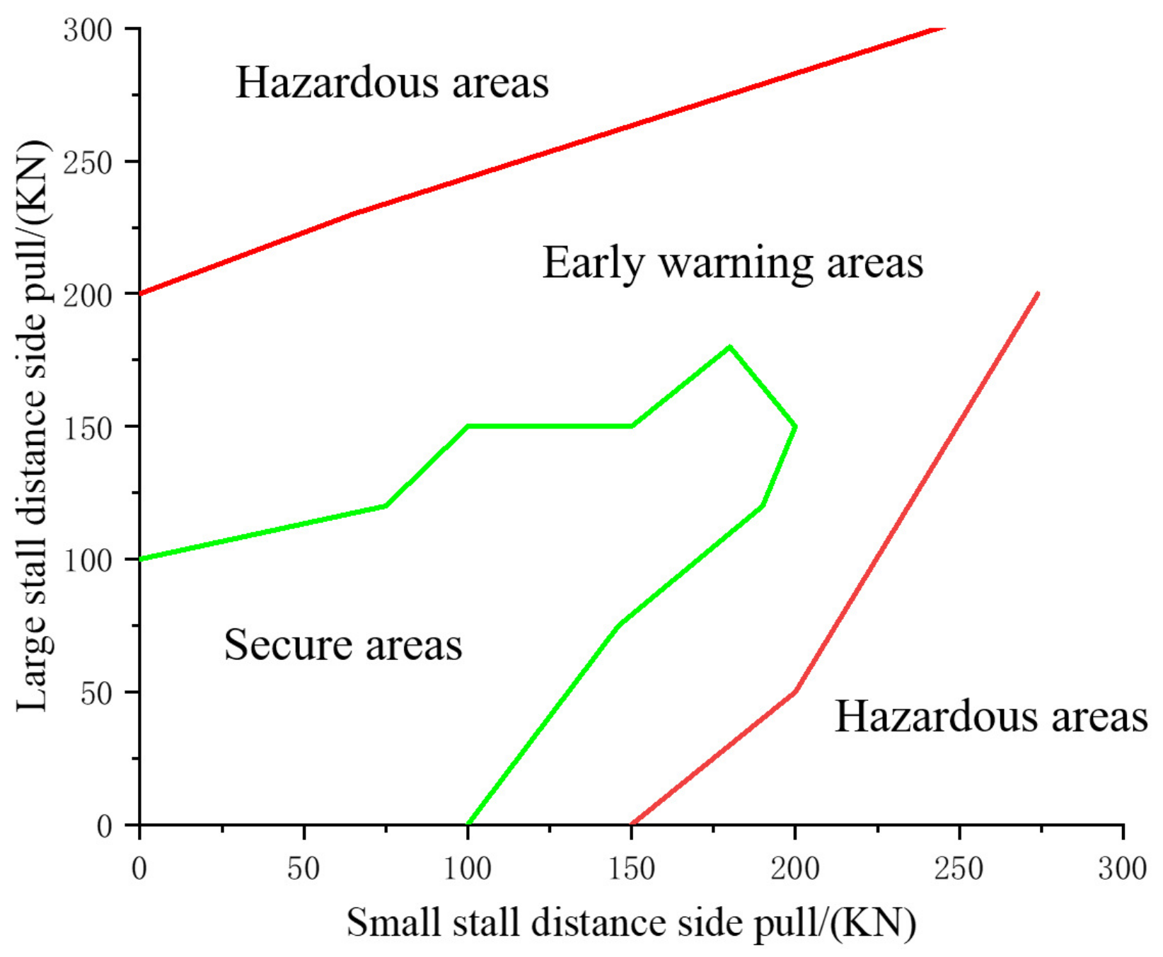
Through the above steady-state and transient analysis, the overall safety of the tower-line system is evaluated, the limit state of the transmission tower is calculated and simulated, and the safety status warning map of the transmission tower is established, which can effectively warn the health status of the transmission tower. According to the characteristics of the model, the key force-bearing points can be selected for reinforcement to prevent the safety accidents of the transmission line. As mentioned above, the force transmission process of the straight tower is the part with the largest axial force bearing.

This research, which was established based on an actual transmission line, needs further verification of its universality. In the future, higher requirements will be placed on the stability and accuracy of numerical simulation.

References

1. Bo, C.; Xinxin, S.; Jingbo, W. Progress in mechanical modeling of power transmission pylon systems. Eng. Mech. 2021, 38, 1–21. [Google Scholar]
2. Zhengliang, L.; Zhengzhi, X.; Feng, H.; Zhitao, Y. Design and wind tunnel testing of an aeroelastic model for the 1000 kV Han River crossing EHV transmission tower system. Chin. Acad. J. Abstr. 2008, 14, 65. [Google Scholar]
3. Eltaly, B.; Saka, A.; Kandil, K. FE Simulation of Transmission Tower. Adv. Civ. Eng. 2014, 2014, 258148. [Google Scholar] [CrossRef] [Green Version]
4. Deng, H.; Xu, H.; Duan, C.; Jin, X.; Wang, Z. Experimental and numerical study on the responses of a transmission tower to skew incident winds. J. Wind. Eng. Ind. Aerodyn. 2016, 157, 171–188. [Google Scholar] [CrossRef] [Green Version]
5. He, B.; Zhao, M.; Feng, W.; Xiu, Y.; Wang, Y.; Feng, L.; Qin, Y.; Wang, C. A method for analyzing stability of tower-line system under strong winds. Adv. Eng. Softw. 2019, 127, 1–7. [Google Scholar] [CrossRef]
6. Liqiang, A.; Zhiqiang, Z.; Renmou, H.; Ronglun, Z.; Songling, P.; Cheng, L.; Wengang, Y. Dynamic response analysis of power transmission tower system under typhoon action. Vib. Shock 2017, 36, 255–262. [Google Scholar]
7. Wenzhe, B.; Li, T. Study on collapse damage of transmission tower-line system under downburst flow. Eng. Mech. 2022, 39, 78–83. [Google Scholar]
8. Yiqin, O.; Haifeng, C.; Deng, Y.; Guohua, C. Study on the power impact effect of ice-covered line dismantling in mountainous areas. J. Wuhan Univ. Technol. 2017, 5, 69–74. [Google Scholar]
9. Roy, S.; Kundu, C.K. Design and analysis of transmission tower under wind loading. In Recent Developments in Sustainable Infrastructure; Springer: Berlin/Heidelberg, Germany, 2021; pp. 231–241. [Google Scholar]
10. Qiang, X.; Jiguo, L.; Chengchong, Y.; Yong, Z. Wind tunnel test study on wind load transfer mechanism of 1000 kV UHV transmission tower system. Chin. J. Electr. Eng. 2013, 33, 109–116. [Google Scholar]
11. Hongnan, L.; Haifeng, B. Wind (rain) induced vibration response and stability of power transmission tower line system. J. Civ. Eng. 2008, 41, 31–38. [Google Scholar]
12. Yan, G.; Jingbo, Y. Wind load calculation method for transmission line towers in micro-terrain areas. Grid Technol. 2012, 36, 111–115. [Google Scholar]
13. Chenguo, Y.; Yu, L.; Zehong, Z.; Chengxiang, L.; Lei, Z.; Zhou, Z. Reliability assessment of ice-covered transmission towers based on ultimate load carrying capacity analysis. High Volt. Technol. 2013, 39, 2609–2614. [Google Scholar]
14. Lun, Y.; Wenjuan, L.; Yong, C.; Dong, Y. Transmission tower line system dance response characteristics test. J. Huazhong Univ. Sci. Technol. Nat. Sci. Ed. 2013, 11, 51–57. [Google Scholar]
15. Chenguo, Y.; Feng, M.; Daolin, X.; Xiaoquan, L.; Zehong, Z.; Yujia, C. Mechanical properties of uneven ice-covered transmission tower line system. High Volt. Technol. 2011, 37, 3084–3092. [Google Scholar]
16. Ra, H.; Li-Ming, W.; Pu-Xuan, Z.; Zhi-Cheng, G. Dynamic calculation of ice-shedding jumps on extra-high voltage lines. Chin. J. Electr. Eng. 2008, 28, 1–6. [Google Scholar]
17. Junke, H.; Jingbo, Y.; Qinghua, L.; Fengli, Y. Ultra/Extra high voltage AC multiple transmission lines with the same tower for ice imbalance tension analysis. Grid Technol. 2011, 35, 33–37. [Google Scholar]
18. Jakubovičová, L.; Sapietová, A.; Moravec, J. Static analysis of transmission tower beam structure. MATEC Web Conf. 2018, 244, 01011. [Google Scholar] [CrossRef] [Green Version]
19. Tian, L.; Pan, H.; Qiu, C.; Ma, R.; Yu, Q. Wind-induced collapse analysis of long-span transmission tower–line system considering the member buckling effect. Adv. Struct. Eng. 2019, 22, 30–41. [Google Scholar] [CrossRef]
20. Al-Bermani, F.G.; Kitipornchai, S. Nonlinear analysis of thin-walled structures using least element/member. J. Struct. Eng. 1990, 116, 215–234. [Google Scholar] [CrossRef]
21. Xiaohui, L.; Lufei, Z.; Bo, Y.; Xiaoyan, Z. Dance mode analysis of continuous ice-covered conductors. J. Syst. Simul. 2016, 28, 8. [Google Scholar]
22. Du, Y.X.; Lu, X.L. Study on the dynamic response of wind-induced ice shedding in power transmission tower line system. J. Hunan Univ. Nat. Sci. Ed. 2015, 42, 7. [Google Scholar]
23. Lou, W.; Zhang, Y.; Xu, H. Analysis of the effect of ice and wind coupling on the dynamic tension and parameters of the de-icing of transmission lines. High Volt. Technol. 2022, 48, 1052–1059. [Google Scholar] [CrossRef]
24. Ibrahim, A.M.; El Damatty, A.A.; Aboshosha, H. Dynamic behaviour of pre-stressed concrete transmission poles under synoptic wind loading. Adv. Struct. Eng. 2022, 25, 685–697. [Google Scholar] [CrossRef]
25. Guohui, S.; Guanghui, Y.; Bingnan, S.; Yunxiang, H.; Wenjuan, L. Simulation of deicing of transmission lines considering deicing velocity effect. J. Chongqing Univ. Nat. Sci. Ed. 2010, 33, 7. [Google Scholar]
26. Fu, X.; Li, H.N. Dynamic analysis of transmission tower-line system subjected to wind and rain loads. J. Wind. Eng. Ind. Aerodyn. 2016, 157, 95–103. [Google Scholar] [CrossRef]
27. Mingxi, Z.; Bo, H.; Wentao, F.; Yu, W.; Lijun, F.; Kun, W.C. Influence of tower-line coupling factors on mechanical properties of high-voltage transmission tower-line structures under ice-cover loading and analysis. Chin. J. Electr. Eng. 2018, 38, 7141–7148+7440. [Google Scholar] [CrossRef]
28. Khalid, H.M.; Ojo, S.O.; Weaver, P.M. Inverse differential quadrature method for structural analysis of composite plates. Comput. Struct. 2022, 263, 106745. [Google Scholar] [CrossRef]
29. Kabir, H.; Aghdam, M. A robust Bézier based solution for nonlinear vibration and post-buckling of random checkerboard graphene nano-platelets reinforced composite beams. Compos. Struct. 2019, 212, 184–198. [Google Scholar] [CrossRef]
Figure 1. Tower-line coupling-system finite element model.
Buildings 13 00828 g001
Figure 2. Transmission tower main material number.
Buildings 13 00828 g002
Figure 3. Single-line diagram of tension-resistant transmission tower (left), single-line diagram of tangent tower (right) (Length unit: mm).
Buildings 13 00828 g003
Figure 4. Ideal elastoplastic double broken line model.
Buildings 13 00828 g004
Figure 5. Analysis of forces on overhanging chain-line wires.
Buildings 13 00828 g005
Figure 6. Transmission tower-line multicritical point wind spectrum history load (left). Comparison of simulated self-power spectrum and calculated self-power spectrum in point 1 (right).
Buildings 13 00828 g006
Figure 7. Ice-shedding load-time curve.
Buildings 13 00828 g007
Figure 8. Tower shaft force in static with no wind.
Buildings 13 00828 g008
Figure 9. Results of axial force calculation for the model with wire under wind–ice load.
Buildings 13 00828 g009
Figure 10. Time course under the vertical direction of ice-shedding displacement.
Buildings 13 00828 g010
Figure 11. Time course under the vertical direction of ice-shedding displacement.
Buildings 13 00828 g011
Figure 12. Displacement in three degrees of freedom at the highest point.
Buildings 13 00828 g012
Figure 13. Time course under the vertical direction of ice-shedding displacement.
Buildings 13 00828 g013
Figure 14. Conductor ice shedding under different span distances where the highest point of transmission towers swing laterally and along the line.
Buildings 13 00828 g014
Figure 15. The maximum tension time range of the conductor when the conductor is deiced under a different line span distance.
Buildings 13 00828 g015
Figure 16. Time history-conductor sag under maximum icing thickness.
Buildings 13 00828 g016
Figure 17. Transmission tower security posture warning map.
Buildings 13 00828 g017