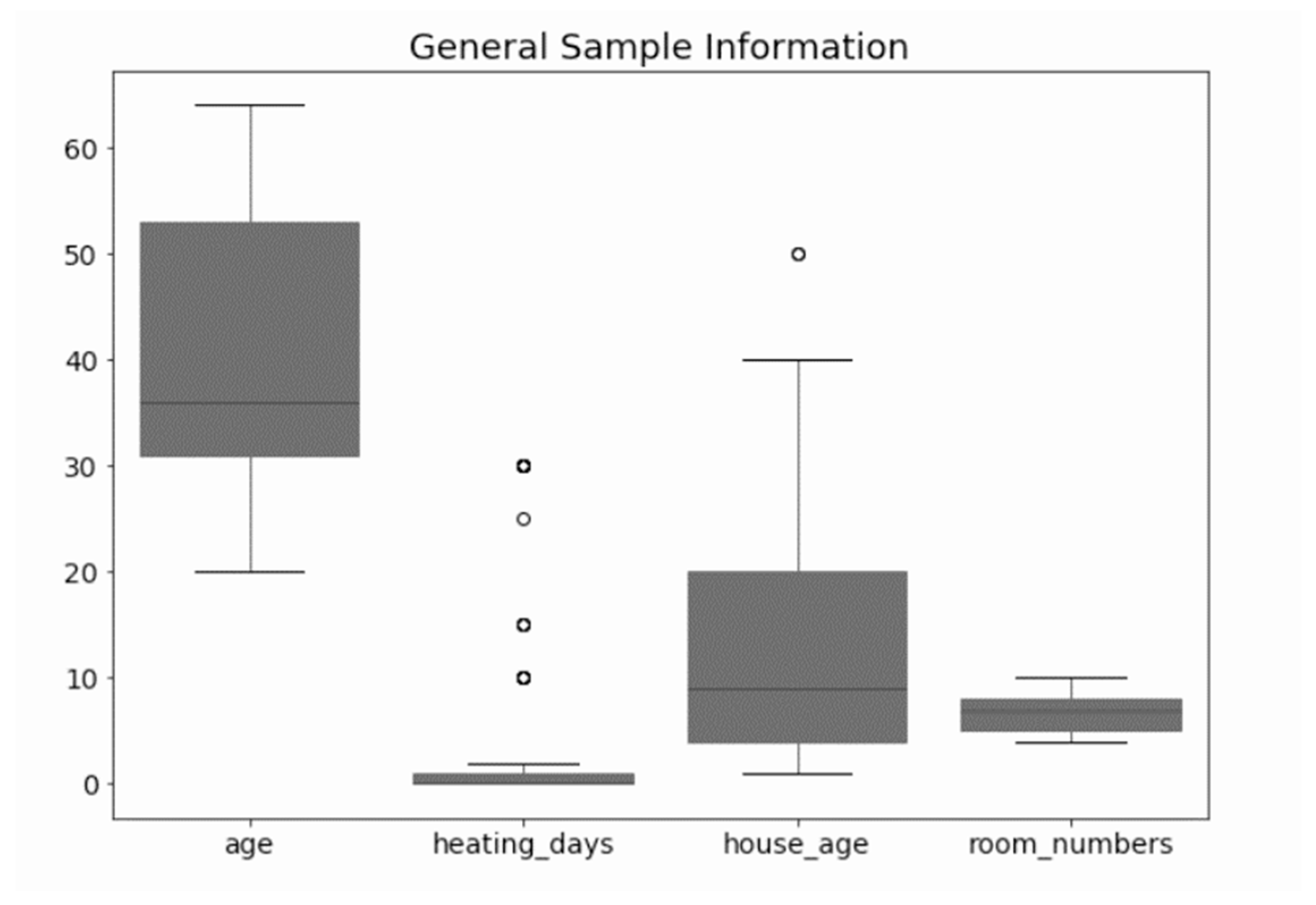
Figure 1.
General information of the selected sample. The figure shows box plots of the information gathered during the fieldwork stage from the sample. The black line within the box represents the mean. The circles represent the outliers.
Figure 1.
General information of the selected sample. The figure shows box plots of the information gathered during the fieldwork stage from the sample. The black line within the box represents the mean. The circles represent the outliers.
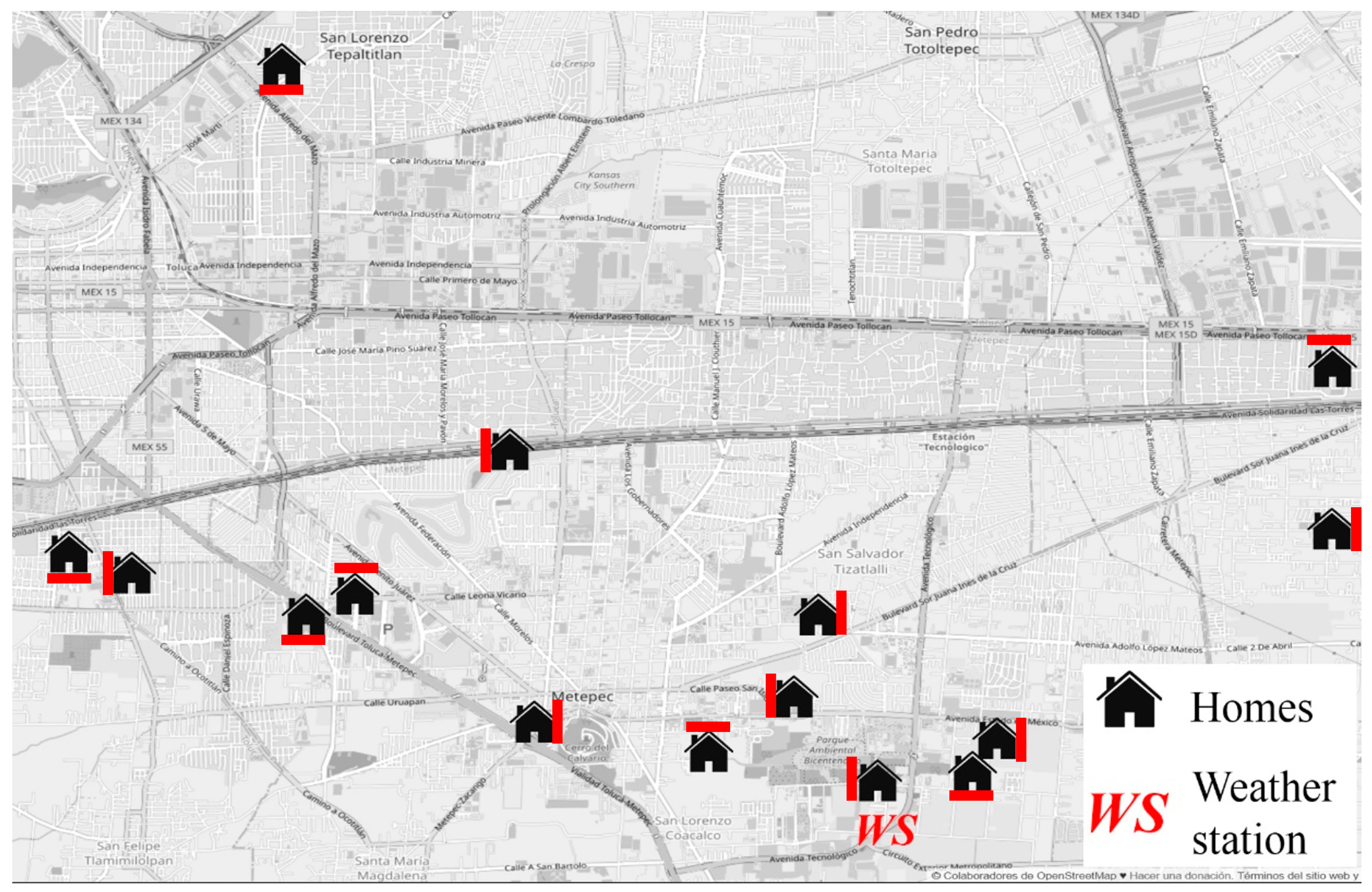
Figure 2.
Location of the participating homes in Toluca and the weather station from which the external climatic data were obtained. Source of the background image was OpenStreetMap
® [
47]. Source of the house icon was. The red line next to the house represents the orientation of the room in which the sensor was positioned.
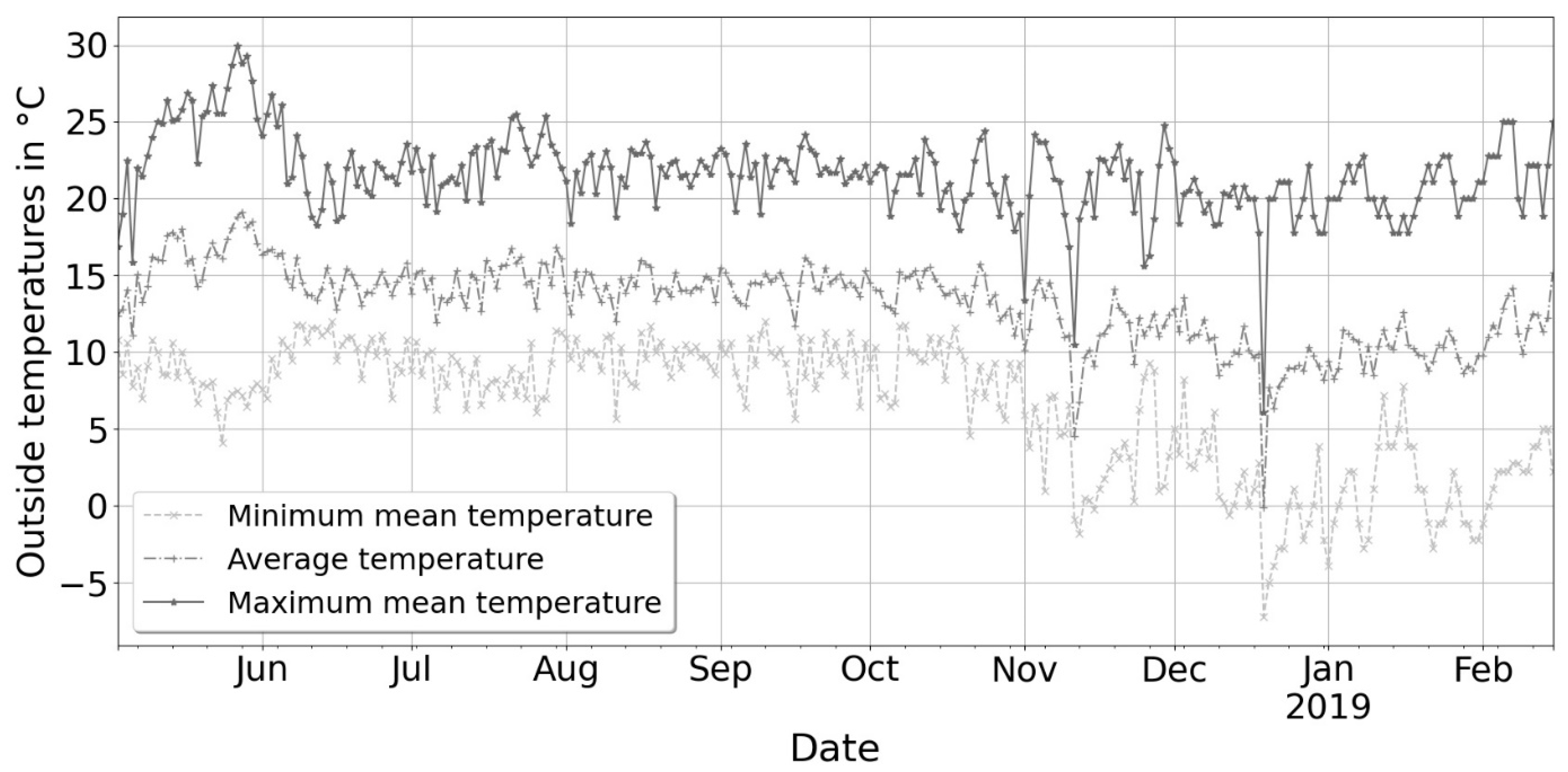
Figure 3.
Daily outdoor temperatures in Toluca from May 2018 to February 2019. Light grey represents the minimum, mid-grey the average, and dark grey the maximum.
Figure 3.
Daily outdoor temperatures in Toluca from May 2018 to February 2019. Light grey represents the minimum, mid-grey the average, and dark grey the maximum.
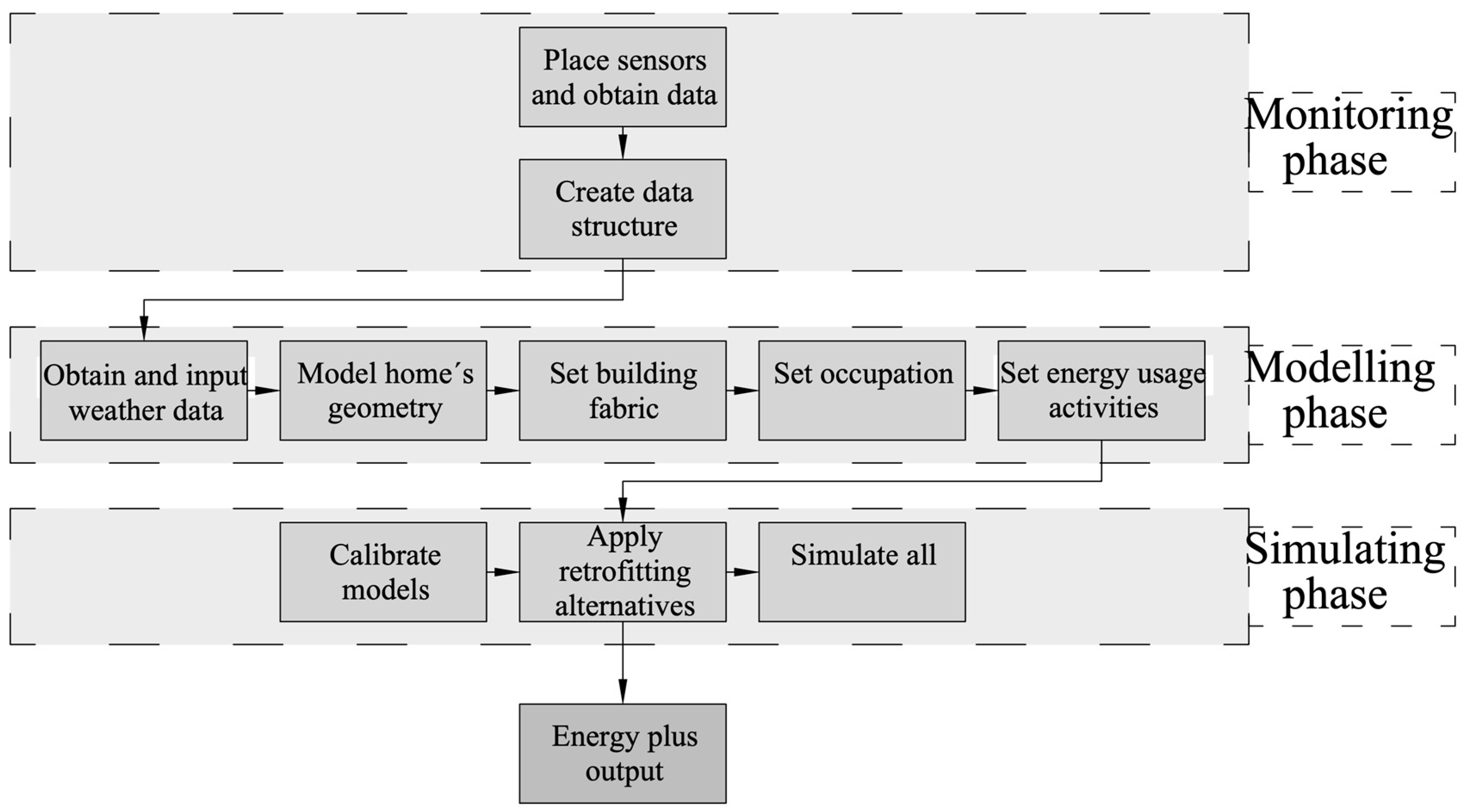
Figure 4.
Stages of the simulation process. Stage 1 (monitoring phase) consisted of obtaining the sensors, ensuring their correct operation, and placement in the different houses. Stage 2 (modelling phase) surveyed the homes (measuring the perimeters and taking photographs). Later, these data were used in D.B. to create the simulation models. Finally, Stage 3 (simulation stage) consisted of simulations with the different building envelopes.
Figure 5.
Section drawings of the different building fabric typologies used in the dynamic simulations. Each cross-section is explained below identified by its letter: (a) as built; (b) double glazing, no insulation; (c) single glazing and 3 cm of insulation (as established by the NOM-ENER-020); (d) single glazing and 5 cm of insulation (standard practice); (e) double glazing and 5 cm of insulation.
Figure 6.
Heatmap of the average of each house’s seasonal living room temperatures across 2018 (spring, summer and autumn) and 2019 (winter).
Figure 6.
Heatmap of the average of each house’s seasonal living room temperatures across 2018 (spring, summer and autumn) and 2019 (winter).
Figure 7.
Hourly living room temperatures for the length of the study (left) and those in the cold season (right). The cold season comprises the period from 1 October to 28 February. The dashed horizontal blue line shows the limit of hours (3%) that the homes must not exceed before meeting the dashed red vertical line, which represents the 18 °C temperature threshold recommended by WHO.
Figure 8.
Ranked living room relative humidity by season. The red dotted line represents the mean.
Figure 8.
Ranked living room relative humidity by season. The red dotted line represents the mean.
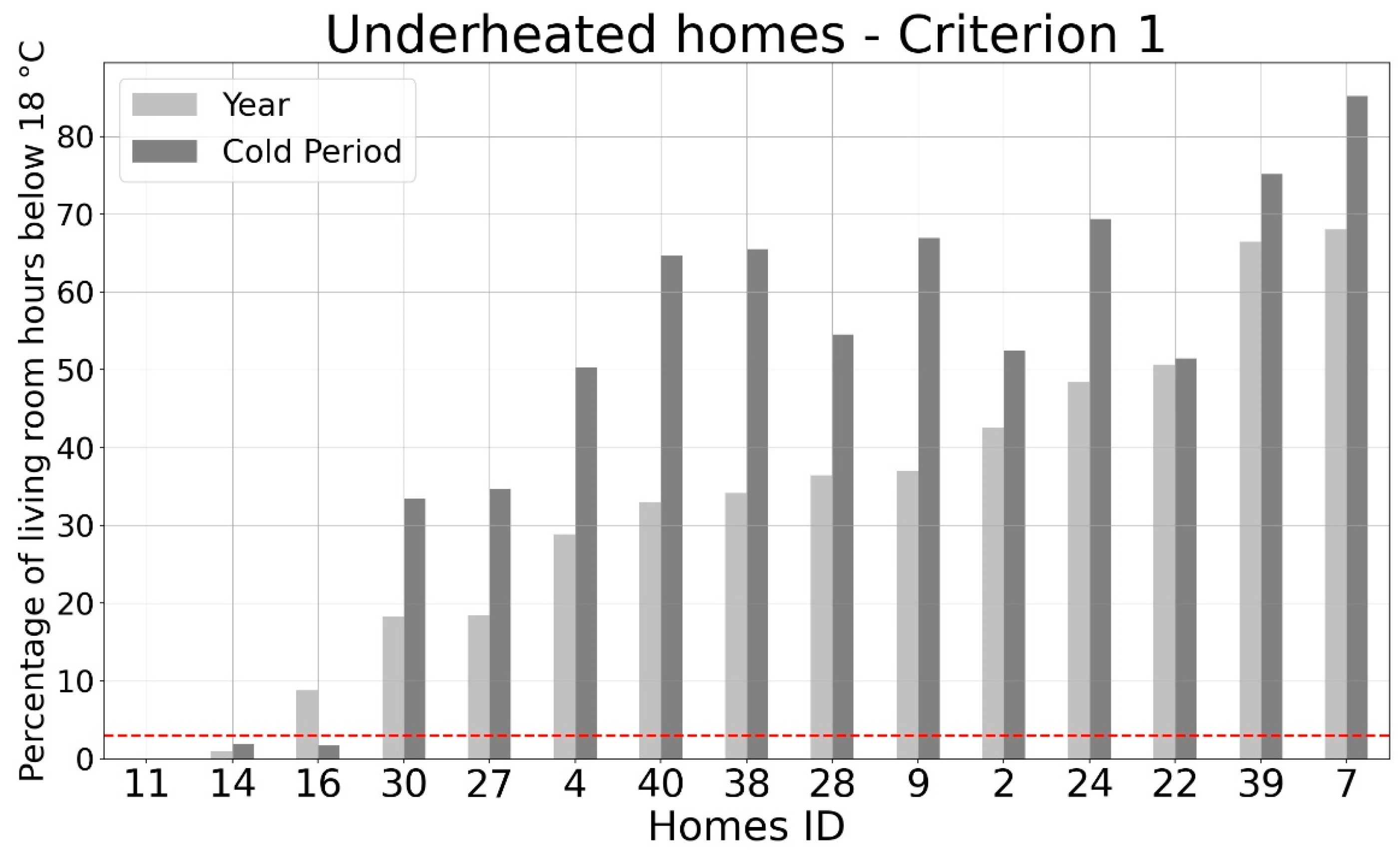
Figure 9.
Percentage of underheated hours according to criterion 1.
Figure 9.
Percentage of underheated hours according to criterion 1.
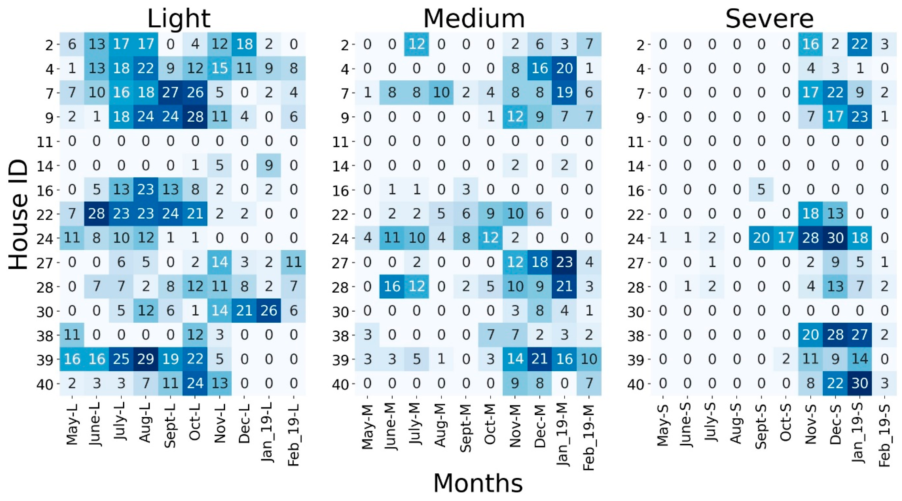
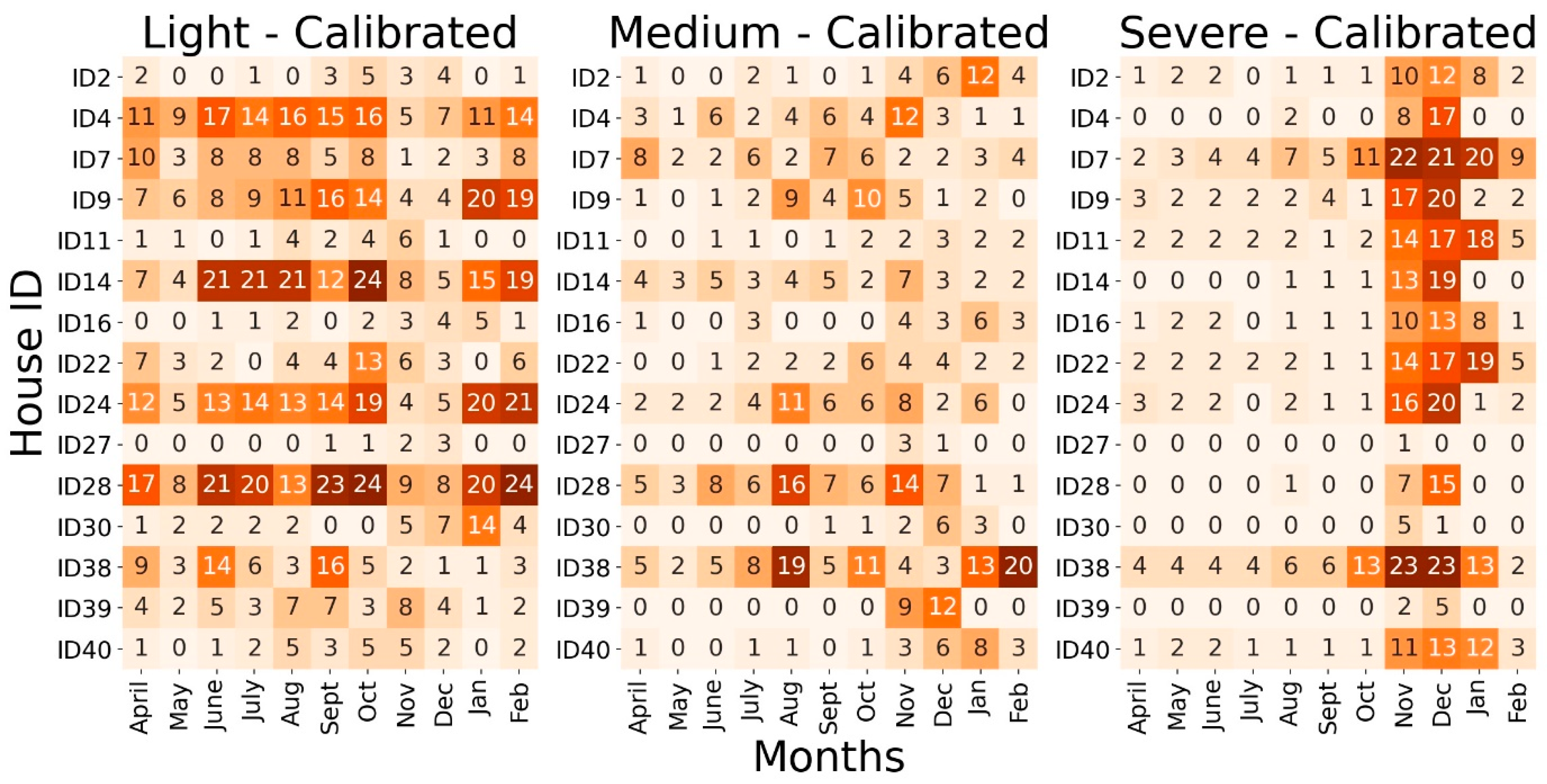
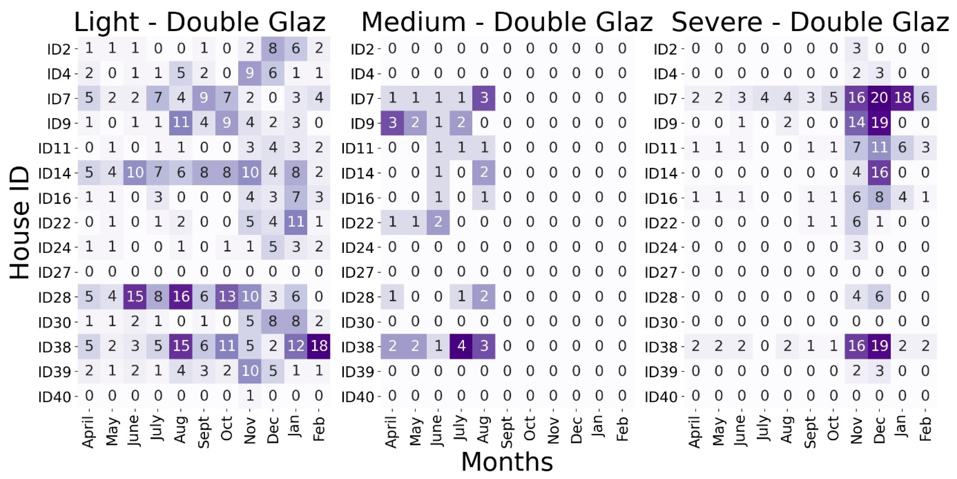
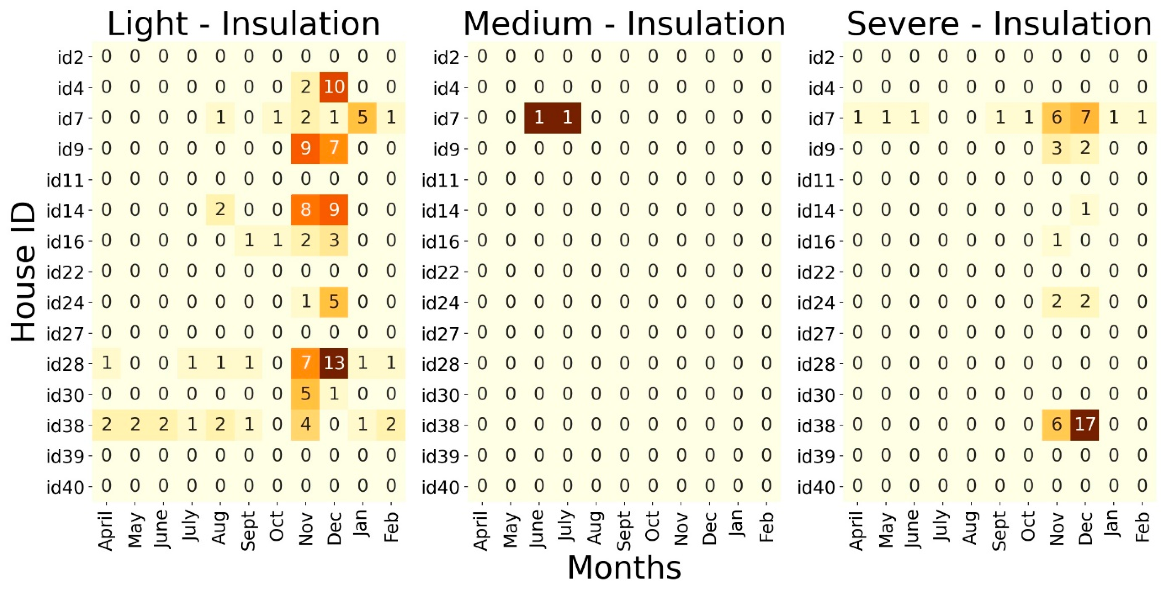
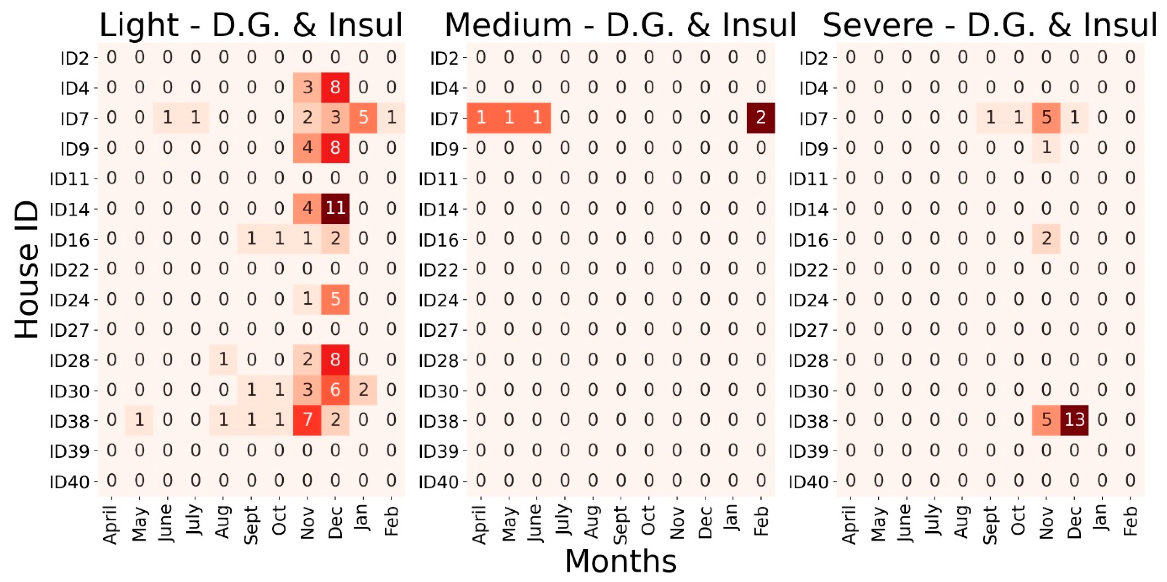
Figure 10.
Number of underheating days per home split monthly according to criterion 2.
Figure 10.
Number of underheating days per home split monthly according to criterion 2.
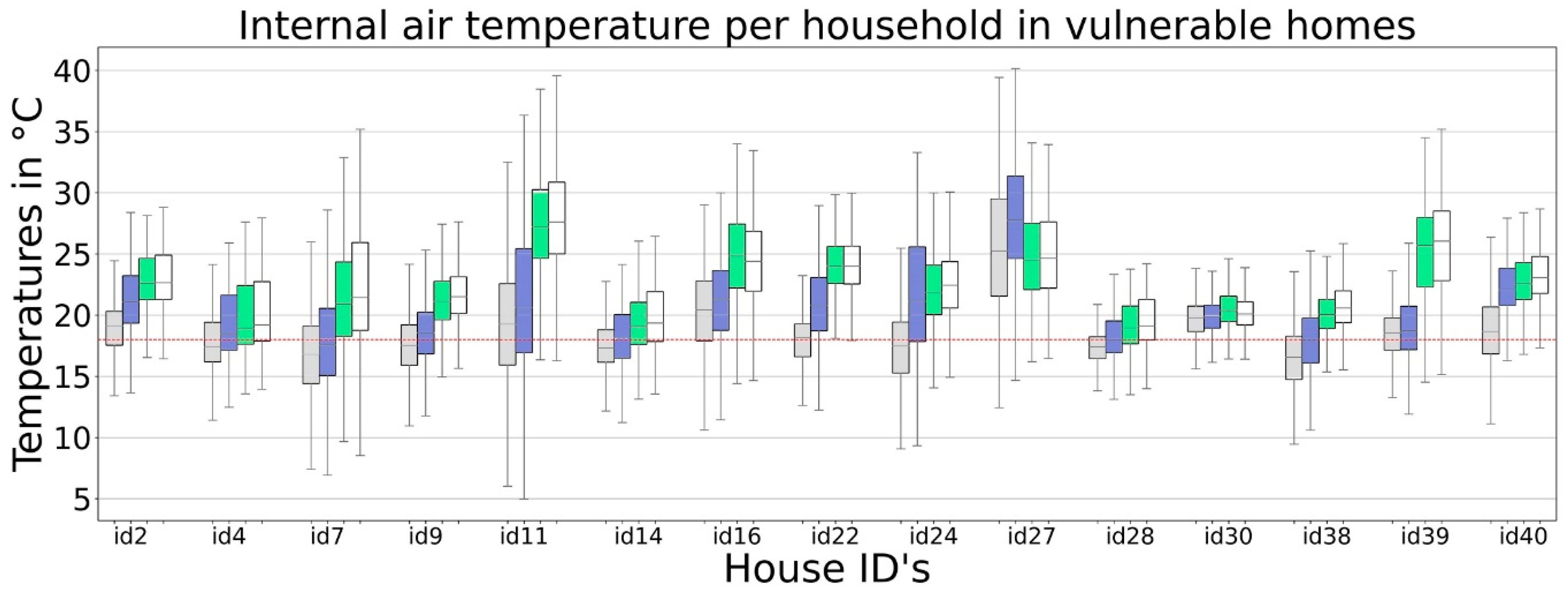
Figure 11.
Boxplots of internal temperatures, where the light grey (first from left to right) corresponds to the temperatures monitored with sensors. The blue boxes (second from left to right) correspond to the simulations with double glazing, the green (third from left to right) to the homes only with insulation, and the white (fourth from left to right) correspond to the ones under the NOM-ENER-021 parameters.
Figure 12.
Adaptive approach graphs showing the outdoor running mean temperatures (°C) (x-axis) and the indoor operative temperature (°C) (y-axis) of the homes included in this study against the parameters established in the ASHRAE 55 standard. The segmented line (inner) represents 90% acceptability. The continuous (external) line represents 80% acceptability ASHRAE thresholds. Finally, the spots represent one hour (monitored or simulated). The top left (grey) shows the monitored (actual) temperatures. The different simulations provide the remaining results, as stated in each graph’s title.
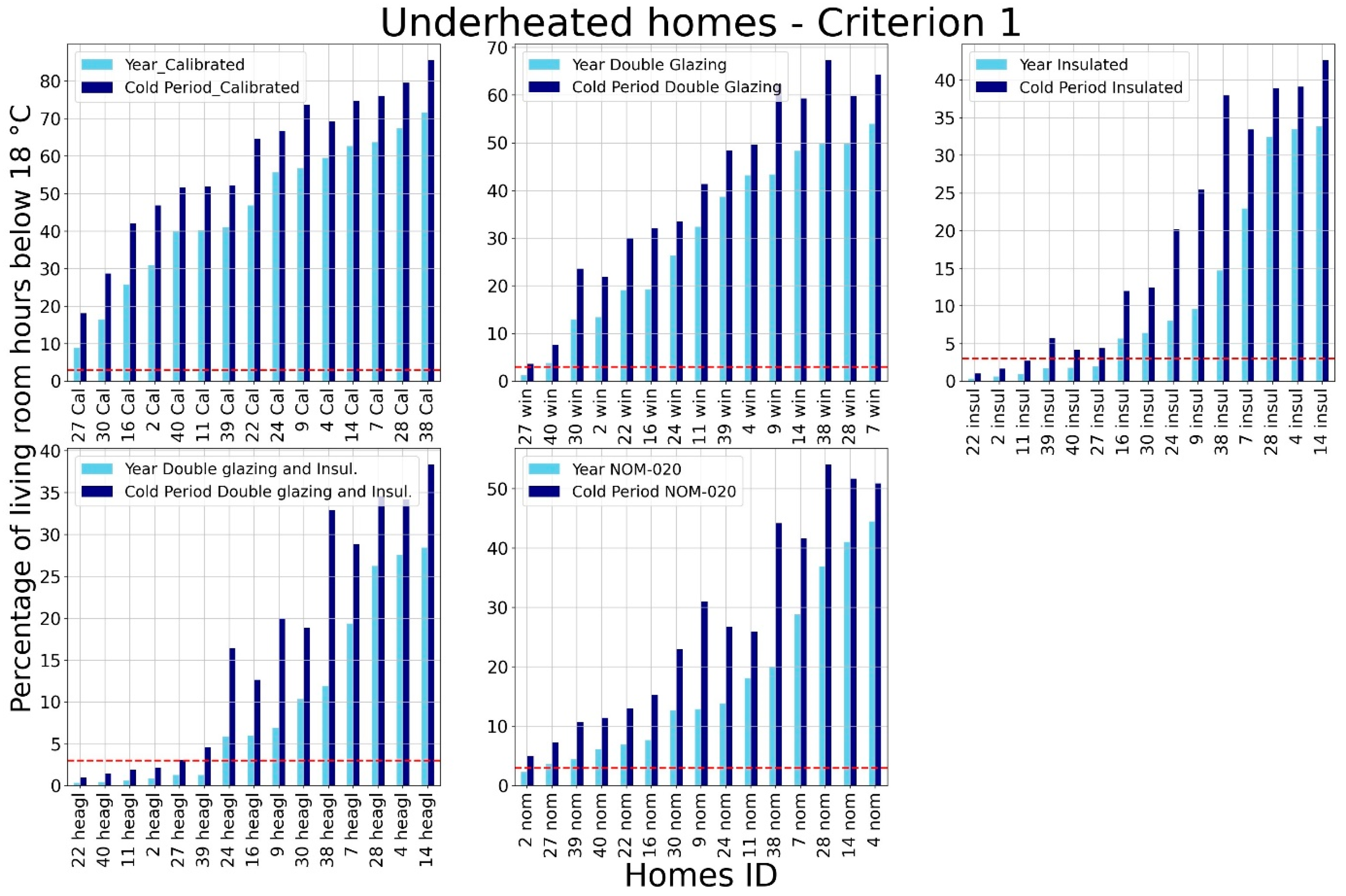
Figure 13.
Percentage of underheated hours according to our criterion 1 after simulations.
Figure 13.
Percentage of underheated hours according to our criterion 1 after simulations.
Figure 14.
Relationships among predictors of average total self-reported health score in the best-fit multiple linear regression model (backward method; R2 = 0.91; Adjusted R2 = 0.88); distinguished by whether predictors are of the environmental origin or personal adaptive strategies. Direct effects are displayed by straight arrows, whereas correlations among predictors are described as curved arrows. Variables composing the PPD index are pictured within a lighter-shaded box (upper-left corner) for informative purposes only.
Table 1.
Diseases caused by poor quality indoor environments according to the WHO.
Table 1.
Diseases caused by poor quality indoor environments according to the WHO.
| Housing Characteristic | Health Impact |
|---|
| Indoor dampness/mould | Asthma onset in children |
| Physical conditions | Home injury |
| Crowding | Tuberculosis |
| Cold | Mortality |
| Noise exposure | Ischemic heart disease |
| Indoor radon | Lung cancer |
| Second-hand smoke | Respiratory infection; asthma; heart disease; lung cancer |
Lead exposure
(e.g., paints) | Anaemia decreased renal function, cognitive, developmental, neurological, behavioural, and cardiovascular effects. |
| Carbon monoxide | CO2 intoxication, tissue hypoxia. |
| Formaldehyde exposure | Respiratory symptoms in children. |
| Indoor smoke from solid fuel use | Pneumonia in children, and chronic obstructive pulmonary disease and lung cancer in adults. |
| Housing quality | Mental health: anxiety, behaviour conduct disorders in children, depression, feelings of inadequacy, social isolation, stigmatisation. |
Table 2.
Sample characteristics.
Table 2.
Sample characteristics.
| Characteristics of the Sample | |
|---|
| Sex | Female | 9 |
| | Male | 6 |
| Age | 20–30 | 6 |
| | 30–40 | 4 |
| | 40–50 | 3 |
| | 50 or more | 2 |
| Qualifications | Undergraduate | 9 |
| | Postgraduate | 4 |
| | Preferred not to answer | 2 |
| Socio-Economic Characteristics | |
| Room numbers | 0–5 | 10 |
| | 5–10 | 5 |
| House age | 0–5 | 7 |
| | 5–10 | 5 |
| | 10 or more | 3 |
| Income | Less than 9000 MXN | 10 |
| | More than 9000 MXN | 5 |
Table 3.
Characteristics of the sensors.
Table 3.
Characteristics of the sensors.
| Parameter | Sensor Model | Range | Accuracy |
|---|
| Temperature | DS18B20 | −10 to +85 °C | >±0.5 °C |
| Relative Humidity | RHT03 | 0–100% | >±2% |
Table 4.
Types of questions and answers included in the “long” surveys deployed during the fieldwork stage.
Table 4.
Types of questions and answers included in the “long” surveys deployed during the fieldwork stage.
| Self-Reported Physical Health | |
|---|
| Participants responded: “Last month I had __ problems” | Responses available |
| Vision | Yes |
| Ear | No |
| Arthritis | Rather not to say |
| Cardiovascular | |
| Hypertension | |
| Respiratory | |
| Neurodegenerative | |
| Depression | |
| Circulatory | |
| Life Satisfaction and Self-worth | |
| Participants responded: “Last month I felt __” | Responses available |
| Happy | Never |
| Confident | Rarely |
| Excited | Sometimes |
| Loved | Often |
| Content | Very often |
| Joyful | Rather not to say |
| Healthy | |
| Life anxiety | |
| Participants responded: “Last month I felt __” | Responses available |
| Nervous | Never |
| Hopeless | Rarely |
| Worthless | Sometimes |
| Restless | Often |
| Powerless | Very often |
| Lonely | Rather not to say |
| Adaptation Style | |
| Participants responded: “Last month when I felt too cold, I __” | Responses available |
| Used extra blankets | Never |
| Wore extra layers | Rarely |
| Drank a hot drink | Sometimes |
| Stayed longer in bed | Often |
| Took a hot shower | Very often |
| Left the cold room | Rather not to say |
| Self-perceived physical capacity | |
| Participants responded: “Last month I could __” | Responses available |
| Walk half kilometre | Extremely difficult |
| Climb ten steps | Moderately difficult |
| Stand for two hours | Easy |
| Bend over kneel | Manageable |
| Reach something above head level | Very easy |
| Carry a supermarket bag | Rather not to say |
| Pull furniture | |
| Go out to socialize | |
Table 5.
Scores assigned to the different answer options in the group of questions regarding life-satisfaction and worth.
Table 5.
Scores assigned to the different answer options in the group of questions regarding life-satisfaction and worth.
| Option | Score Assigned |
|---|
| Never | 0 |
| Rarely | 2 |
| Sometimes | 3 |
| Often | 4 |
| Very often | 5 |
| Rather not say | 1 |
Table 6.
Scores assigned to the different answer options in the group of questions regarding physical capacity.
Table 6.
Scores assigned to the different answer options in the group of questions regarding physical capacity.
| Option | Score Assigned |
|---|
| Extremely difficult | 1 |
| Moderately difficult | 2 |
| Easy | 3 |
| Manageable | 4 |
| Very easy | 5 |
Table 7.
U-Values in
for each building fabric configuration used in dynamic simulations. The letters at the top of the table correspond to the sections shown in
Figure 5.
Table 7.
U-Values in
for each building fabric configuration used in dynamic simulations. The letters at the top of the table correspond to the sections shown in
Figure 5.
| Building Element | (a) | (b) | (c) | (d) | (e) |
|---|
| Wall |
2.97 |
2.97 |
0.91 |
0.56 |
0.56 |
| Roof |
3.06 |
3.06 |
0.89 |
0.57 |
0.57 |
| Window |
6.12 |
3.15 |
6.12 |
6.12 |
3.15 |
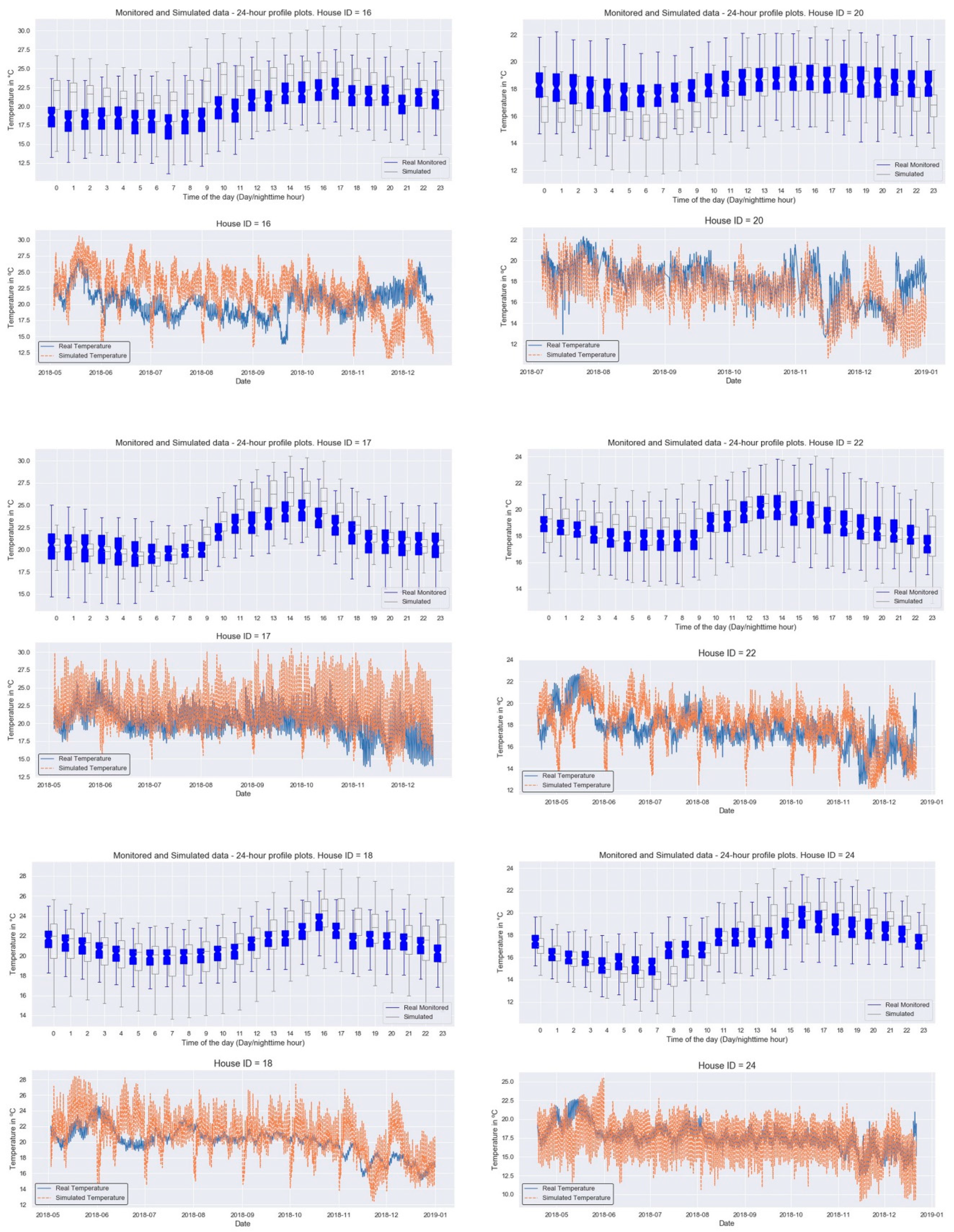
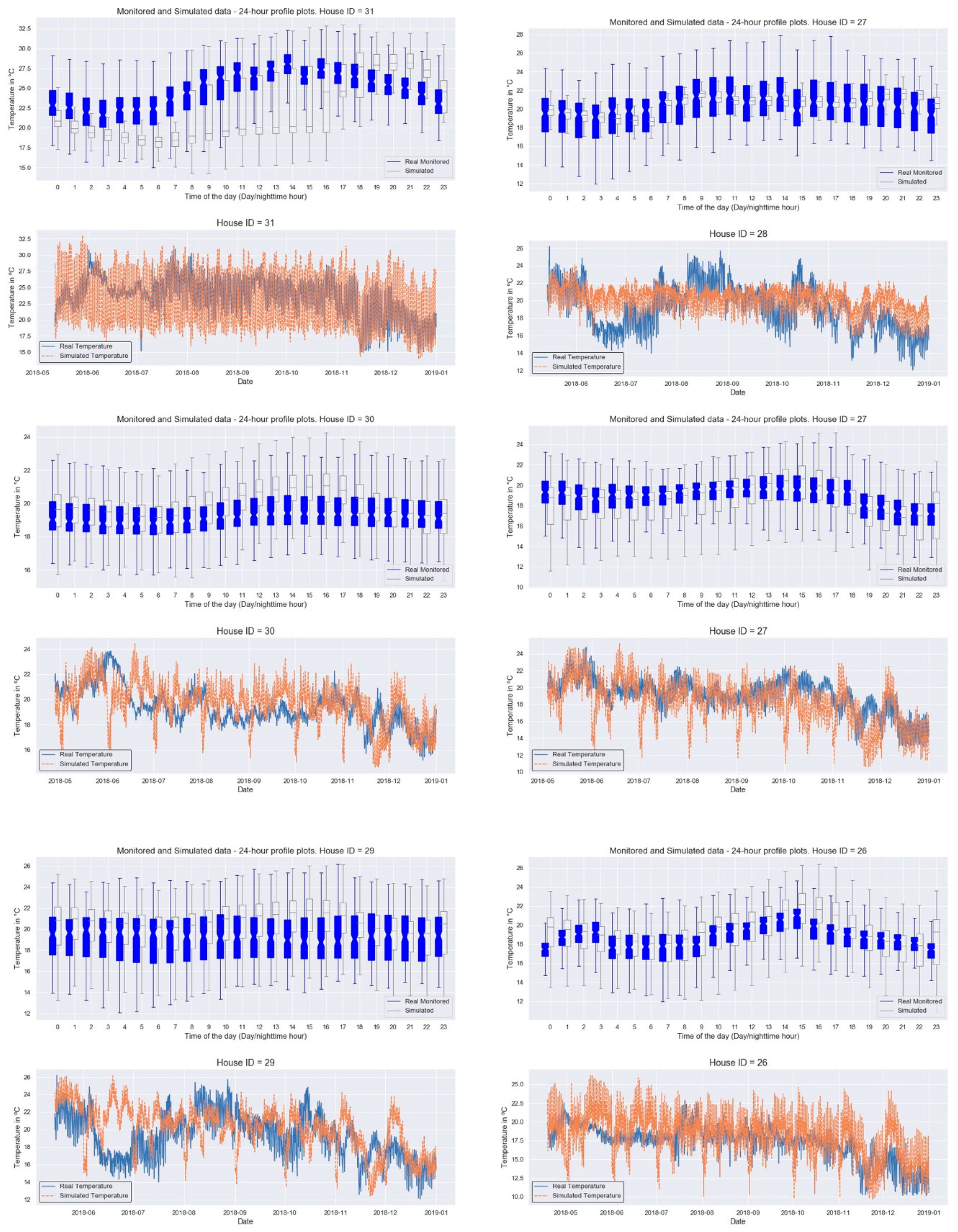
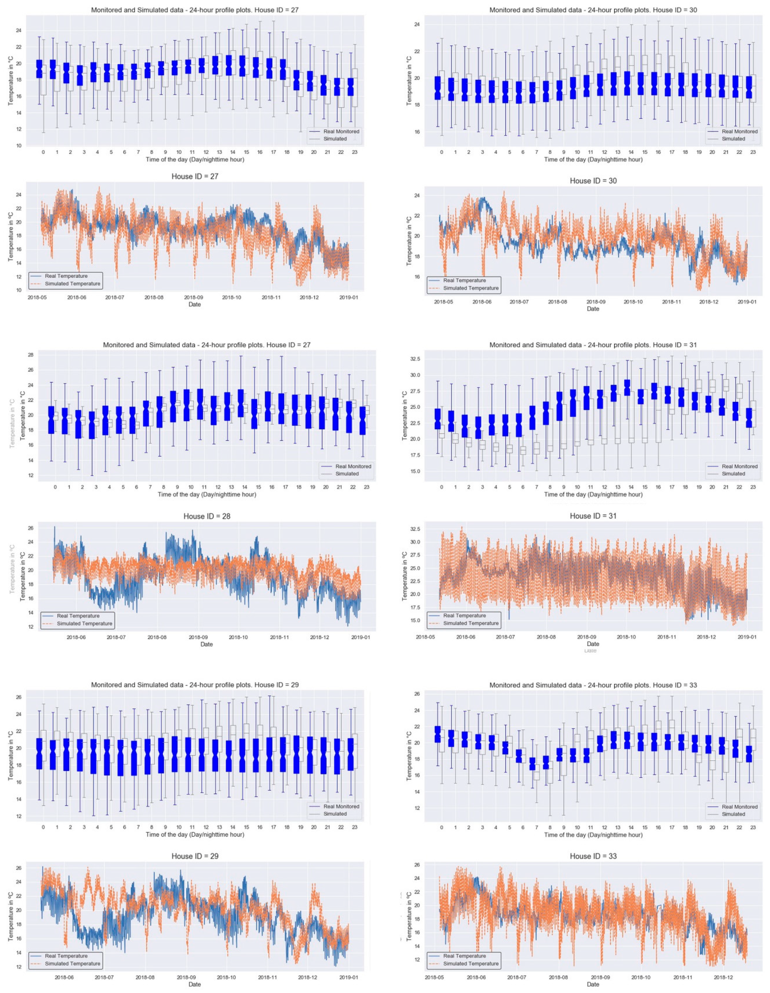
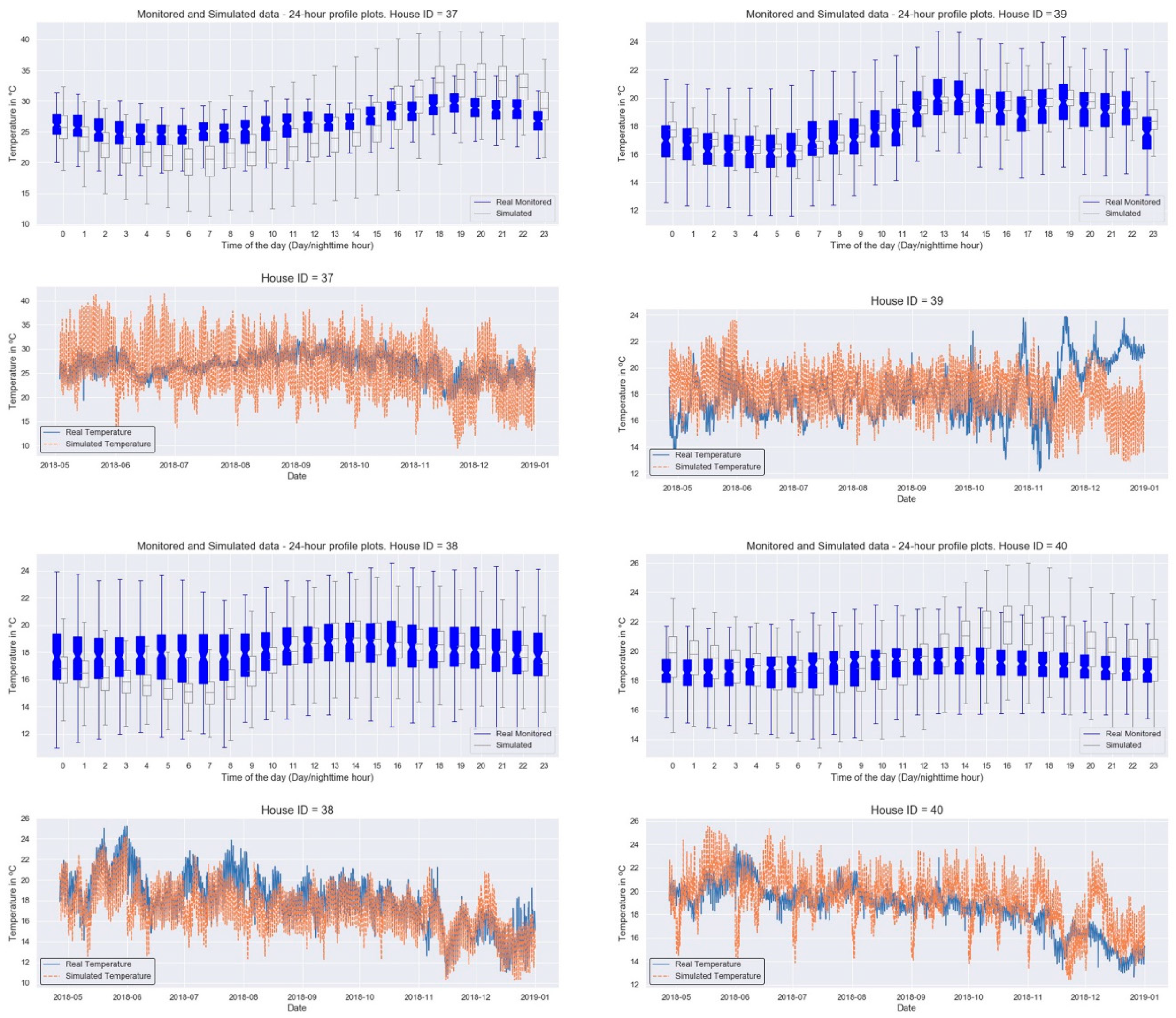
Table 8.
Mean Bias Error (MBE) and Root Mean Square Error (RMSE) comparing the calibrated temperatures provided by our sensors against those provided by the Design-Builder model.
Table 8.
Mean Bias Error (MBE) and Root Mean Square Error (RMSE) comparing the calibrated temperatures provided by our sensors against those provided by the Design-Builder model.
| | ID_2 | ID_3 | ID_4 | ID_6 | ID_7 | ID_14 | ID_16 | ID_17 | ID_18 | ID_20 | ID_22 | |
|---|
| MBE | 10.08 | 12.88 | 12.8 | 7.79 | 12.43 | 20.32 | 16.47 | 12.34 | 9.65 | 11.16 | 9.69 | |
| RMSE | 12.69 | 19.32 | 13.7 | 9.96 | 14.08 | 20.05 | 20.61 | 18.44 | 12.81 | 12.76 | 12.22 | |
| | ID_24 | ID_26 | ID_27 | ID_28 | ID_29 | ID_30 | ID_31 | ID_33 | ID_37 | ID_38 | ID_39 | ID_40 |
| MBE | 14.22 | 12.64 | 11 | 10.66 | 12.31 | 7.11 | 18.29 | 12.35 | 21.48 | 10.98 | 13.03 | 9.02 |
| RMSE | 15.81 | 16.41 | 12.78 | 13.32 | 16.37 | 9.03 | 19.5 | 15.53 | 22.34 | 13.09 | 16.39 | 11.72 |
Table 9.
Example of monitored hourly temperature data.
Table 9.
Example of monitored hourly temperature data.
| Hour | 00:00 | 01:00 | 02:00 | 03:00 | 04:00 | 05:00 | 06:00 | 07:00 |
|---|
| Temperature in °C | 16 | 16 | 16 | 16 | 15 | 16 | 17 | 18 |
| Hour | 08:00 | 09:00 | 10:00 | 11:00 | 12:00 | 13:00 | 14:00 | 15:00 |
| Temperature in °C | 19 | 20 | 20 | 21 | 23 | 23 | 21 | 21 |
| Hour | 16:00 | 17:00 | 18:00 | 19:00 | 20:00 | 21:00 | 22:00 | 23:00 |
| Temperature in °C | 21 | 20 | 18 | 18 | 18 | 17 | 17 | 16 |
Table 10.
Average days per month with light, medium and severe underheating. D G stands for double glazing.
Table 10.
Average days per month with light, medium and severe underheating. D G stands for double glazing.
| | | Calibrated | Double Glazing | Insulation | D G and Insul | NOM-020 |
|---|
| Light | mean | 6.5 | 3.1 | 0.7 | 0.6 | 1.3 |
| sd | 1.8 | 1.1 | 1 | 1 | 1.2 |
| Medium | mean | 3.5 | 1.3 | 0.3 | 0.3 | 0.7 |
| sd | 1.2 | 1.2 | 0.6 | 0.5 | 1.2 |
| Severe | mean | 4.1 | 1.6 | 0.3 | 0.1 | 0.6 |
| sd | 4.1 | 2.2 | 0.6 | 0.3 | 1 |
Table 11.
Summary of survey results per house ID, for each of the variables used in multiple regression analyses.
Table 11.
Summary of survey results per house ID, for each of the variables used in multiple regression analyses.
| House ID | Mean Predicted Percentage Dissatisfied (PPD) | Median Added Adaptation Score | Mean Total Health Problems Score | Median Life Satisfaction and Worth Self-Reported Score | Days w/Underheating | House Age | Respondent’s Age | Mean Physical Self-Perception Score | Mean Life Anxiety Self-Reported Score | Mean Predicted Mean Vote (PMV) |
|---|
| 2 | 31.37 | 15 | 2.67 | 7 | 134 | 10 | 60 | 27.66 | 7 | −0.76 |
| 4 | 27.02 | 20 | 2 | 7 | 92 | 50 | 55 | 30.33 | 6 | −0.85 |
| 7 | 23.06 | 15 | 3 | 6.5 | 220 | 20 | 32 | 30.33 | 3.67 | −0.65 |
| 9 | 12.48 | 19 | 1.75 | 6.25 | 108 | 15 | 44 | 34.75 | 3 | −0.6 |
| 11 | 12.88 | 16 | 1.8 | 5 | 0 | 30 | 31 | 39.4 | 2.2 | −0.11 |
| 14 | 27.89 | 14.5 | 4 | 3.25 | 2 | 6 | 31 | 33.5 | 4.5 | −0.41 |
| 16 | 11.11 | 12 | 2 | 7 | 20 | 10 | 24 | 37 | 3.5 | −0.43 |
| 22 | 10.25 | 15 | 3.6 | 3.5 | 176 | 20 | 52 | 37.4 | 5 | −1.03 |
| 24 | 6.78 | 10 | 2.5 | 5 | 156 | 30 | 33 | 29.5 | 6 | −0.08 |
| 27 | 48.89 | 18 | 4.33 | 6 | 71 | 20 | 60 | 45 | 5 | −1.45 |
| 28 | 23.8 | 14 | 2.5 | 7 | 115 | 15 | 32 | 30.25 | 2.75 | −0.62 |
| 30 | 5.17 | 6 | 1.66 | 6.5 | 61 | 30 | 49 | 41.33 | 5.67 | −0.05 |
| 38 | 9.73 | 8 | 2.8 | 4.5 | 114 | 3 | 30 | 33.4 | 7 | −1.03 |
| 39 | 14.7 | 4 | 3 | 6 | 217 | 15 | 27 | 30.33 | 5.67 | −0.35 |
| 40 | 12.7 | 4 | 3.66 | 4 | 103 | 25 | 63 | 36.33 | 9 | −0.23 |
| Mean ± SD | 18.52 ± 11.74 | 12.70 ± 5.20 | 2.75 ± 0.85 | 5.63 ± 1.32 | 105.93 ± 68.95 | 19.93 ± 11.90 | 41.53 ± 13.69 | 34.43 ± 4.95 | 5.06 ± 1.85 | −0.58 ± −0.40 |
Table 12.
Best-fit final stepwise linear regression (backward) model with average total self-reported health problems score as the dependent variable for 15 homes in the city of Toluca, State of Mexico, Mexico.
Table 12.
Best-fit final stepwise linear regression (backward) model with average total self-reported health problems score as the dependent variable for 15 homes in the city of Toluca, State of Mexico, Mexico.
| | Predictor | B | SE | StB | t | p | Tolerance | VIF |
|---|
| (Constant) | | 4.47 | 0.37 | | 12.87 | >0.01 | | |
| | Median Life satisfaction and worth self-reported score | −0.45 | 0.061 | −0.71 | −7.51 | >0.01 | 0.91 | 1.10 |
| | Median added adaptation score | −0.053 | 0.018 | −0.32 | −2.94 | 0.015 | 0.66 | 1.51 |
| | Average PPD | 0.06 | 0.008 | 0.89 | 8.21 | >0.01 | 0.69 | 1.44 |
| | Total days w/Underheating | 0.003 | 0.001 | 0.25 | 2.68 | 0.023 | 0.93 | 1.07 |
Table 13.
Excluded variables for the best-fit final stepwise linear regression (backward) model with average total self-reported health problems score as the dependent variable for the data of 15 homes in the city of Toluca, State of Mexico, Mexico.
Table 13.
Excluded variables for the best-fit final stepwise linear regression (backward) model with average total self-reported health problems score as the dependent variable for the data of 15 homes in the city of Toluca, State of Mexico, Mexico.
| | Beta in | t | p | Partial
Correlation | Tolerance | VIF |
|---|
| House Age | −0.91 | −0.96 | 0.36 | −0.30 | 0.905 | 1.106 |
| Respondent’s Age | −0.018 | −0.18 | 0.86 | −0.059 | 0.847 | 1.181 |
| Average Physical self-perception score | 0.131 | 1.25 | 0.24 | 0.384 | 0.699 | 1.431 |
| Mean Life anxiety self-reported score | −0.087 | −0.71 | 0.498 | −0.229 | 0.563 | 1.777 |
| Average (PMV) | −0.137 | −1.03 | 0.328 | −0.326 | 0.461 | 2.172 |


